MANUSCRIPT
Authors:	Alexander Tank and Alan A. Stocker
Affiliation:	Department of Psychology and
	Department of Electrical and Systems Engineering
	University of Pennsylvania
Correspondence:	Dr. Alan A. Stocker
	Computational Perception and Cognition Laboratory
	3401 Walnut Street 313C
	Philadelphia, PA 19104-6228
	U.S.A.
	astocker@sas.upenn.edu
	phone: +1 215 573 9341
Journal:	arXiv
Classification:	Quantiative Biology (Neurons and Cognition)

Biased perception leads to biased action: Validating a Bayesian model of interception

Alexander Tank and Alan A. Stocker

Abstract

We tested whether and how biases in visual perception might influence motor actions. To do so, we designed an interception task in which subjects had to indicate the time when a moving object, whose trajectory was occluded, would reach a target-area. Subjects made their judgments based on a brief display of the object’s initial motion at a given starting point. Based on the known illusion that slow contrast stimuli appear to move slower than high contrast ones, we predict that if perception directly influences motion actions subjects would show delayed interception times for low contrast objects. In order to provide a more quantitative prediction, we developed a Bayesian model for the complete sensory-motor interception task. Using fit parameters for the prior and likelihood on visual speed from a previous study we were able to predict not only the expected interception times but also the precise characteristics of response variability. Psychophysical experiments confirm the model’s predictions. Individual differences in subjects’ timing responses can be accounted for by individual differences in the perceptual priors on visual speed. Taken together, our behavioral and model results show that biases in perception percolate downstream and cause action biases that are fully predictable.

1 Motivation

Bayesian models of perceptual inference explain many perceptual biases [1, 2, 3]. By leveraging prior knowledge, Bayesian inference provides a principled and optimal strategy for an observer to infer the state of a perceptual variable from observed noisy evidence. Perceptual biases arise in this context because prior beliefs about the environmental statistics influence the perceptual process. Well documented examples include biases cue combination [1], low contrast biases in perceived speed [2], and biases towards the cardinals in orientation perception [4, 5], to name a few. A separate line of work suggests that many visual illusions fail to lead to equivalent biases in motor behavior [6]. For example, the Ponzo illusion, where lines of the same length are perceived differently due to receding distance, does not translate into differences in motor commands for grasping these lines [7]. From a Bayesian perspective, the disconnect between perception and action appears puzzling. If a perceptual illusion can be explained in the context of optimal Bayesian inference, then we would expect the illusion to translate into biased behavior because the Bayesian framework is grounded in the statistics of the physical world [8]. Furthermore, why allocate costly resources for optimal perception if these perceptions are not used in guiding actions?

Speed perception has been extensively studied within the Bayesian framework [2] and provides an entry point for dissecting the influence of Bayesian perception upon action. Speed perception is traditionally studied with a two alternative forced choice task (2AFC), where subjects must choose the faster of two motion stimuli. Under this setup, low contrast stimuli are perceived to move slower relative to high contrast stimuli of the same speed [9]. A prior distribution favoring slower speeds combined with a wider likelihood width for low contrast qualitatively explains the slow speed illusion and provides a tight fit to 2AFC data [2, 3].

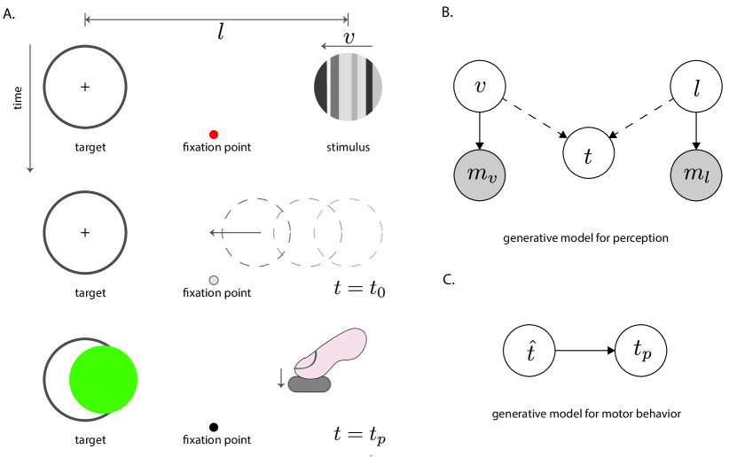
Figure 1: Interception task: task structure and generative model. (A) (top) Subjects fixate on the small red dot on the bottom of the screen while viewing a drifting motion stimulus [2] for 1s at an eccentricity of $6^{\circ}$. (middle) At the moment the motion stimulus disappears, the fixation dot turns white to alert the subjects that the stimulus has been released. The stimulus moves, occluded, at a constant speed across the screen. (bottom) Subject makes a button press to indicate when the stimulus would have reach the center of the target area. For medium contrast conditions, feedback was provided indicating the end position of the stimulus at the time of the bottom press. Position was shown in green if the stimulus is within the target area and in red otherwise. (B) The generative model for perception shown as a directed graph. The values of the latent physical variables, stimulus velocity, $v$, and length, $l$, are combined using a simple physics model (deterministic) to define a time, $t$, for the stimulus to reach the target area. Observed variables represent the sensory measurements for speed, $m_{v}$, and length, $m_{l}$. The width of the noise distribution for $m_{v}$ is contrast dependent and changes based on the contrast from trial to trial. (C) The generative model for the motor control assumes that the time of the key press (action), $t_{p}$, is drawn from a Gaussian distribution with mean equal to the perceptual time estimate, $\hat{t}$. Solid arrows indicate stochastic dependencies whereas dotted lines indicate deterministic dependencies.

We developed a sensory-motor interception task in order to assess whether or not these perceptual speed biases translate to biases in timing actions. In this interception task subjects briefly view a moving grating stimuli contained in a circular window (Figure 1). The stimuli then disappears at which point it moves occluded with constant velocity across the screen. Subjects are instructed to make a button press when they believe the stimuli has crossed to the other side of the screen and coincides with some target a fixed distance away from stimulus presentation. Importantly, the moving stimuli are of differing contrasts to induce the slow speed illusion. We also present different speeds to obtain timing data for multiple speed contrast pairs. To formalize a clear hypothesis, we developed a Bayesian model for this task that assumes that a subject’s timing response is optimal in order to best most accurately intercept the object in the target area. Such an optimal model necessarily predicts that the perceptual biases (because they are optimal) translate to the corresponding motor biases.

In what follows we first derive the Bayesian model for our the described interception task. We then explain how we perform the task with human subjects and present the measured behavioral results. Finally we compare the data to predictions of our model based on prior and likelihood parameters obtained from psychophysical experiments in a previous study of speed perception.

2 Interception model

We assume each subject observes both the speed of the moving stimulus and the distance between the stimulus and the target (see Fig. 1A). These separate perceptual measurements must be integrated and decoded in some sensible way in order to determine an adequate time estimate. We formalize perception, intuitive physics, and action in our task using generative models and then derive an optimal time estimator based on assumptions of rationality, the independence assumptions of our perceptual model, and the motor noise in timing actions.

2.1 Generative model for perception

We model each trial independently, and in what follows we avoid trial subscripts for convenience. On each trial the stimulus speed, $v$, and length between stimulus center and target, $l$, are each drawn independently from their respective natural prior distributions, $p(v)$ and $p(l)$. The time, $t$, the stimulus needs to reach the center of the target is dependent only on the physical speed and length and is thus drawn from the conditional distribution, $p(t|v,l)$. Speed, length, and time are the latent variables that we combine in a vector ${\bf h}=\{v,l,t\}$. The observable variables ${\bf m}=\{m_{v},m_{l}\}$, are the noisy sensory measurements of the true speed and length and are each drawn independently from their conditional distributions, $p(m_{v}|v)$ and $p(m_{l}|l)$. Taken together, these conditional and prior distributions define a generative model over the observable variables, ${\bf m}$, and latent physical variables, ${\bf h}$. The joint distribution for each trial becomes:

$$p({\bf m},{\bf h})=p(v)p(l)p(m_{v}|v)p(m_{l}|l)p(t|v,l)$$

and is displayed graphically in Figure 1. The observer has access to only the measurements and must infer the physical state. The posterior distribution of the physical variables given the measurements is:

$$p({\bf h}|{\bf m})=\frac{p(m_{v}|v)p(v)p(m_{l}|l)p(l)p(t|v,l)}{p(m_{v})p(m_{l})}\\ =p(v|m_{v})p(l|m_{l})p(t|v,l)$$

where the marginal $p(m_{v},m_{l})$ = $p(m_{v})p(m_{l})$ because the physical sources of the measurements are independent. Furthermore, we see that the marginal distribution for latent physical variables is separable into independent posterior distributions for speed and length and the conditional distribution for time.

2.2 Physics model

We embed the physical relationship between time, velocity and length in the conditional distribution $p(t|v,l)$. If we assume that length and velocity are constant, rather than fluctuating due to some unknown latent forces, the conditional density becomes deterministic:

$$p(t|v,l)=\delta(t,q(v,l))$$

where $\delta$ is the Dirac delta measure that assigns all of its probability mass to the second argument. The function $q(v,l)$ is the physics model which maps speed and length to time. Because we assume constant speed and length, the physics model is the simple Newtonian relationship: $q(v,l)=\frac{l}{v}$.

2.3 Action model

The timing decision, $\hat{t}({\bf m})$, is a deterministic function of both length and speed measurements. We assume the subject has only indirect control over its motor commands, in the sense that the produced motor output, $t_{p}$, stochastically depends on the perceptual estimate $\hat{t}({\bf m})$ via the distribution $p(t_{p}|\hat{t}({\bf m}))$ (Figure 1). We model $p(t_{p}|\hat{t}({\bf m}))$ as a Gaussian distribution with mean $\mu_{p}=\hat{t}({\bf m})$ and standard deviation that grows proportionally with the mean, $\sigma_{p}=w_{p}\mu_{p}$ where $w_{p}$ is the time production Weber fraction [10].

2.4 Estimator of travel time

We model timing action choice in our task using decision theory [11], which allows us to identify an optimal estimator from a class of functions, $f({\bf m})$, that maps the set of measurements directly onto a timing decision. We assume subjects operate rationally and try to accrue as much task dependent reward as possible. Thus our optimal estimator, $\hat{t}({\bf m})$, is one which minimizes the posterior loss between the timing actions, $t_{p}$, that depend stochastically on the timing estimate, and the latent physical variables:

$$\hat{t}({\bf m})=\underset{f({\bf m})}{\operatorname{argmin}}\int\mathcal{L}({\bf h},f({\bf m}))p({\bf h}|{\bf m})\,d{\bf h}$$

where $\mathcal{L}$ is the the expected penalty for making the timing decision $f({\bf m})$ in physical state ${\bf h}$ and $p({\bf h}|\bf{m})$ is the posterior distribution of our generative model. Of course, in our model the timing actions depend stochastically on the timing decision so $\mathcal{L}$ is determined by integrating over all possible timing actions:

$$\mathcal{L}({\bf h},f(m))=\int L({\bf h},t_{p})p(t_{p}|f(m))\,dt_{p}$$

where $L({\bf h},t_{p})$ is the exact loss for performing action $t_{p}$ in latent state ${\bf h}$ and $p(t_{p}|f({\bf m}))$ is the probability of performing motor command $t_{p}$ under time decision $f({\bf m})$, as defined above.

While interception actions are performed in time, actions are chosen in reference to the distance moved by the object. We thus decompose the loss function, $L$, into two separate functions that measure loss along different dimensions:

$$L({\bf h},t_{p})=L_{L}({\bf h},t_{p})+\eta L_{T}({\bf h},t_{p})$$

Where $L_{L}$ measures loss in distance, $L_{T}$ measures loss in time, and $\eta$ parameterizes the weight of loss in time with respect to loss in distance. A natural form for loss in distance is the squared error between the true length, $l$, and the distance traveled at time press $t_{p}$:

$$L_{L}({\bf h},t_{p})=\big{(}l-vt_{p}\big{)}^{2}$$

where $vt_{p}$ is the distance traveled by the stimulus moving at speed $v$ at time $t_{p}$. This loss function captures the motivational thrust of our task: to land the moving stimulus as close to the target center as possible. We also assume that subjects prefer shorter timing actions to finish the experiment quickly. The loss function in time then takes a linear form:

$$L_{T}({\bf h},t_{p})=t_{p}$$

Under these loss functions $\eta$ controls the trade off between task performance and completion time. With these model specifications, one can show that the optimal estimator that minimizes the posterior loss is given by:

$$\hat{t}({\bf m})=f_{opt}({\bf m})=\frac{E(l|m_{l})E(v|m_{v})-\frac{\eta}{2}}{(w_{p}^{2}+1)E(v^{2}|m_{v})}$$

where $E(l|m_{l})$ and $E(v|m_{v})$ are the expectations of the posterior distributions for $l$ and $v$ respectively and $w_{p}$ is the timing noise fraction. To derive this expression we plug the full loss function and posterior distribution into the expected posterior loss and then find the minima of the resulting expression. We first integrate through each term:

$$Loss =\iint\Big{(}l^{2}-2lvt_{p}+v^{2}t_{p}^{2}+\eta t_{p}\Big{)}p(t_{p}|f({\bf m}))dt_{p}p({\bf h}|{\bf m})\,d{\bf h}$$

$$=\int l^{2}p(l|m_{v})dl-2\iiint lvt_{p}p(t_{p}|f({\bf m}))p(v|m_{v})p(l|m_{l})\,dv\,dl\,dt_{p}$$

$$+\iint v^{2}t_{p}^{2}p(v|m_{v})p(t_{p}|f({\bf m}))\,dv\,dt_{p}+\int\eta t_{p}p(t_{p}|f({\bf m}))dt_{p}$$

$$=E(l^{2}|m_{l})+\eta f({\bf m})-2f({\bf m})E(l|m_{l})E(v|m_{v})+E(v^{2}|m_{v})(w_{p}^{2}f({\bf m})^{2}+f({\bf m})^{2})$$

where we have used the fact that probability distributions integrate to one and that the first and second moments of a distribution are the mean and variance plus mean squared, respectively. We note that the final expression is quadratic in $f({\bf m})$ and thus take the derivative of the above equation with respect to $f({\bf m})$, set it equal to zero, and solve for $f({\bf m})$ to obtain the desired result. We now describe our experiment and behavioral results before returning to model specifications needed to predict behavior.

3 Psychophysical experiment

On each trial subjects are presented with a circular patch which contains a horizontal drifting grating. See Figure  1 for example stimuli and [2] for stimulus specifics. The patch is $3^{\circ}$ in radius and is located $5.2^{\circ}$ to the right of the center of the screen. Subjects are told to fixate on a small red circle $3^{\circ}$ below the center of the screen. A large target ring, $4^{\circ}$ in radius, is located $5.2^{\circ}$ to the left of screen center with a small cross in its center. These distances were chosen to ensure that the eccentricity between fixation and stimulus are identical to previous work, $6^{\circ}$. After one second of motion, the grating disappears and the red fixation circle turns white to indicate that the stimuli trajectory has begun. Subjects make a button press when they believe the center of the stimuli coincides with the center of the target (Figure  1).

Subjects first complete two training blocks with feedback at .3 contrast level to adapt to the task. The remaining blocks contain seven different speeds, equally tiled between 3 to 10 $\frac{deg}{s}$, at three contrast levels, high (.8), medium (.3), and low (.1). Feedback remains for medium contrast trials. Three male subjects ages, 23 to 40, completed the task. Subject 1 completed 48 trails for each contrast speed pair while Subjects 2 and 3 completed 90 trials.

To assess the effects of contrast and speed on both the bias and noise in timing actions we first pool trials of the same contrast speed pair to obtain a sample distribution over timing actions, ${\bf t}_{v,c}=\{{t_{1:v,c},...,t_{n:v,c}\}}$, where $v$ and $c$ indicate the speed and contrast and $n$ is the number of trials for each condition. We then compute three sample statistics for each contrast speed pair: the mean, the variance, and the skewness. By comparing mean estimates we can determine the bias in timing actions due to contrast. The variance provides a measure of how the variability in motor behavior is affected by the perceptual noise due to contrast. Skewness, measured as the third standardized moment, is another statistic we apply to compare model and data characteristics. Finally, we calculate sample statistics for an average subject by pooling timing actions across subjects. We do this for both statistical power and for comparison to model predictions with average parameter values.

For the average subject there is significant difference in timing actions ($p\ll.05$) between medium and low contrast and between medium and high contrast stimuli at all speed levels. Lower contrast stimuli lead to longer times than medium contrast and medium contrast leads to longer times than high contrast (Figure  2). Individual subject data portrays a similar result (Figure  3). Subject 1 shows a significant difference between times for medium and low contrast at the slower speeds but not for the two fastest tests speeds. Inspection of the timing plots shows that there is a contraction in the bias between medium and low contrast at higher speeds. Subject 2 shows no contraction in bias and maintains significant difference between conditions at higher speeds. For all subjects the variance decreases as speed increases and is higher for lower contrast than medium and high contrast. These effects are reflected in the average subject plots (Figure  2). For skewness, no clear trend between contrasts is discernible yet overall skewness increases as speed increases.

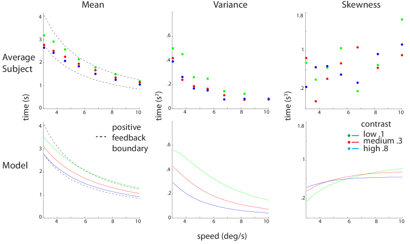
Figure 2: Interception model qualitatively matches average subject data across timing distribution statistics. (top) Combined timing data for all three subjects. For each contrast speed pair the sample mean, sample variance, and sample skewness were determined from the pooled data. (bottom) Model timing results using an average extracted speed prior distribution and likelihood widths (see [2]). Model and data both display a consistent contrast dependent timing bias, whereby lower contrast leads to longer times. Variability is also contrast dependent and the model predicts both the general shape and the range of variance values. The model reproduces the upward trend in skewness and the range of skewness values. Parameters: $s=.65$ $\eta=6$.

4 Model simulations

Our interception model is general and can be applied to a variety of tasks. In what follows we adapt this model to predict behavior in our psychophysical experiment. The model accounts for both the differences in timing bias at low, medium, and high contrasts and the individual subject differences in bias contraction at high speeds.

As mentioned earlier, the prior and conditional distribution for speed have been previously fit to five different subjects [2]. We predict behavior for these subjects by plugging in the fit parameter values to our model. Overall we make behavioral predictions for two of the subjects from the Stocker and Simoncelli 2006 paper, referred to as Subject 1S and Subject 2S, and predictions for an average subject with average parameters taken across all five subjects. We then compare predicted behavior to human performance by computing the expected value, variance, and skewness of the simulated timing distributions. We first flesh out the specifics of the prior and conditional distribution for speed.

4.1 Speed prior and conditional distribution

While the physical speed distribution across the human retina has yet to be measured, human prior distributions for speed have previously been extracted from subjects and show a power law shape [2]. We parameterize this speed prior by assuming the density in physical space is approximately constant for slow speeds, drops as a power law for medium to high speeds, and then transitions back to a constant regime at very high speeds (adapted from [3]):

$$p(v)\propto\frac{1}{(|v|^{2}+b^{2})^{d}}+r\vspace{-.0099in}$$

where $b$ controls at what speed the density transitions from a constant function of speed to a power law, $d$ controls the rate of decay, and $r$ controls at what speed the prior transitions back to constant density. We assume this prior distribution is fixed in advance and is not modulated by the speeds viewed in our experiment. To obtain the parameters for our simulations we fit this parameterized form of the speed prior to the nonparametric prior distributions extracted for each of the five subjects.

We now specify an appropriate speed representation for the observer. We choose a mapping function, $f(v)$, which maps the linear physical speed to a normalized logarithmic speed, $\tilde{v}$ which is in the same space as the perceptual measurement for speed, $m_{v}$. The speed transformation is: $\tilde{v}=f(v)=\log(\frac{v}{v_{o}}+1)$ where $v_{o}$ is a small normalization constant. Working in this space allows us to model the conditional speed observation function, $p(m_{v}|v)$, as a Gaussian distribution with mean $\tilde{v}$. The standard deviation at each speed is separable into functions for the contrast of the stimuli, $c$, and speed: $\sigma(c,\tilde{v})=g(c)h(\tilde{v})$. The speed and contrast likelihood parameters are either set to those previously obtained for each subject or linearly interpolated from these values. Our experiment uses the same distance for every trial so we assume that the subject posterior distribution over length can be approximated by a delta function, $\delta(l,l_{o})$, where $l_{o}$ is the true distance between stimuli and target. The expectation over length becomes $l_{o}$.

4.2 Motor adaptation and model output

Subjects were trained with feedback on stimuli of medium contrast. Due to the slow speed illusion, this leads them (and our model) to overestimate the time it takes for the stimuli to reach the target. After sufficient feedback, timing behavior for medium contrast shifts to faster, more correct, times. To model this motor adaptation on a fast time scale we introduce a scaling factor, $s$, that shrinks the time estimate appropriately to obtain a new corrected time estimate, $\hat{t}_{c}({\bf m})$. Namely, $\hat{t}_{c}({\bf m})=s\,\hat{t}({\bf m})$. Because this adaptation happens quickly it should only affect motor output and not the estimator, which we assume has been optimized by the observer over a lifetime of interacting with moving objects and making time judgments. For simulations the $s$ parameter is chosen such that the mean timing predictions at medium contrast overlap with the veridical time to contact. The timing noise fraction, $w_{p}$, was previously fit to subject timing behavior [10] and we set it to the average of these maximum likelihood fits, $w_{p}$ = $.07$.

In order to compare the timing distributions of the data to our model we computed the probability of making action $t_{p}$ under speed $v$ by marginalizing out the measurements:

$$p(t_{p}|v)=\int p(t_{p}|\hat{t}_{c}(m_{v}))p(m_{v}|v)dm_{v}$$

where $p(t_{p}|\hat{t}_{c}(m_{v}))$ and $p(m_{v}|v)$ are as defined above. The expected value, variance, and skewness of the timing distribution are all calculated using numerical integration.

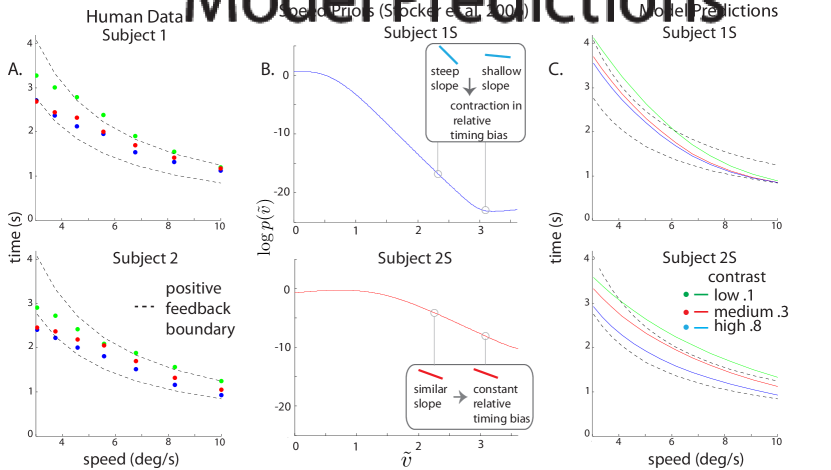
Figure 3: Variance in previously extracted subject priors explains between subject variance in timing actions. (A.) Mean timing actions for Subjects 1 and 2 as functions of speed for each contrast. Subject 2 maintains a roughly constant difference in bias between the contrast levels across speeds while Subject 1 shows a contraction in timing bias. (B.) The extracted parameterized speed prior distribution for both model subjects. The Subject 1S prior slope becomes shallow at high speeds while the Subject 2S prior maintains a constant slope. (C.) Mean timing model predictions for the same two subjects. Again, we see a contraction in timing bias for Subject 1S and not for Subject 2S which can be partially explained by differences in prior shape. Parameters: 1S $s=.9$ $\eta=8$ 2S: $s=.8$ $\eta=6.4$

4.3 Model results and comparison to data

The predictions for the average subject show a clear contrast dependent timing bias qualitatively similar to results from the average human subject. Furthermore, both model and data show no contraction at higher speeds. The model variance predictions across contrasts show a steep initial decline followed by a leveling off at higher speeds. Lower contrasts induce more variability in timing response, as expected due to the wider width of the conditional distribution for speed measurements. This prediction is also qualitatively similar to our human data and within the same variance range. At slow speeds lower contrast stimuli predict smaller skewness while as the speeds increase we see a gradual cross over whereby at high speeds this pattern is reversed. While the raw human data is hard to interpret, both data and model show a shallow but consistent increase in skewness as speed increases.

Predictions for individual subjects reveals key variation in model behavior that is lost when we look at predictions for an average subject. Timing predictions for Subject 1S show a strong contraction in the timing bias at higher speeds, quite similar to the experimental data from Subjects 1 and 3. Predictions for Subject 2S shows no such contraction, and appears qualitatively similar to Subject 2 from our experiment. The difference in subject timing behavior at high speeds can be accounted for by differences in the shape of the prior distribution. Stocker and Simoncelli [2] show that under some conditions the speed bias is proportional to the slope of the prior distribution in the normalized logarithmic space. The slope of the prior for Subject 1S flattens out at faster speeds while the Subject 2S prior maintains a constant slope across speeds (Figure  3). We see that this difference in prior is reflected by a contraction in timing bias for Subject 1S and no contraction in bias for Subject 2S. This suggests that the qualitative differences in human timing response at high speeds can be partially explained by differences in the prior shape.

5 Discussion

Experimentally, we show that the contrast speed visual illusions is reflected in timing actions. To support our conclusion we constructed an interception model grounded in a detailed Bayesian model for speed and showed that our model produces similar biases in timing actions. We argued that differences in timing biases across subjects can be partially explained by differences in the shape of the prior distribution, further strengthening the link between Bayesian perception on the one hand and actions on the other. The qualitative link between the model variance and subject variance and the similar upward trend in skewness shows that most of the behavioral noise is explained by the noise parameters in our model: the motor noise that grows proportionally with timing magnitude and the perceptual noise due to contrast. These results challenge the notion that visual illusions are not reflected in action [6] and demands a more nuanced view. Our results suggest that visual illusions that can be explained in terms of Bayesian inference will similarly affect action.

Our modeling framework for the interception task draws inspiration from recent Bayesian models of human intuitive physics [12, 13]. These models combine uncertainty over physical variables, based on perception and prior knowledge, with a deterministic Newtonian physics model to infer the most likely behavior of the physical world. We expand on this work by investigating a simple speed timing task in detail and thus show that biases in one component of a physics model can percolate through to affect inference about other physical variables, such as time. In future work we intend to teach subjects novel physical relationships and see if speed biases continue to influence judgments about other physical variables.

Over all, we see this work as part of an ongoing effort to probe the degree to which Bayesian models generalize across different behavioral tasks. Our results indicate that the Bayesian model for speed perception generalizes to novel task domains that are different from the one it was originally conceived and that the speed prior transfers across these domains.

Acknowledgments

We thank all the subjects who participated in the experiments. This work was made possible by the Office of Naval Research (grant N00014-11-1-0744).

References

- [1] David Knill. Robust cue integration: A Bayesian model and evidence from cue conflict studies with stereoscopic and figure cues to slant. Journal of Vision, 7, 2007.
- [2] Alan Stocker and Eero Simoncelli. Noise characteristics and prior expectations in human visual speed perception. Nature Neuroscience, 9, 2006.
- [3] James Hedges, Alan Stocker, and Eero Simoncelli. Optimal inference explains the perceptual coherence of visual motion stimuli. Journal of Vision, 11, 2011.
- [4] Odelia Schwartz, Terrance Sejnowski, and Peter Dayan. A Bayesian framework for tilt perception and confidence. Advances in Neural Information Processing Systems 18, 2005.
- [5] Ahna Girshick, Michael Landy, and Eero Simoncelli. Cardinal rules: visual orientation perception reflects knowledge of environmental statistics. Nature Neuroscience, 14, 2011.
- [6] David Westwood and Melvyn Goodale. Converging evidence for diverging pathways: Neuropyschology and psychophysics tell the same story. Vision Research, 51, 2011.
- [7] Tzvi Ganel, Michael Tanzer, and Melvyn A. Goodale. A double dissociation between action and perception in the context of visual illusions: opposite side effects of real and illusory size. Psychological Science, 19, 2008.
- [8] Wilson Giesler and Randy Diehl. A Bayesian approach to the evolution of perceptual and cognitive systems. Cognitive Science, 27, 2002.
- [9] Peter Thomson. Perceived rate of movement depends on contrast. Vision Research, 22, 1982.
- [10] Mehrdad Jazayeri and Michael Shadlen. Temporal context calibrates interval timing. Nature Neuroscience, 13, 2010.
- [11] Julia Trommershauser, Laurence Maloney, and Michael Landy. Decision making, movement planning, and statistical decision theory. Trends in Cognitive Science, 12, 2008.
- [12] Jessia Hamrick, Peter Battaglia, and Joshua Tenenbaum. Internal physics models guide probabilistic judgements about object dynamics. Proceedings of the 33rd Annual Conference of the Cognitive Science Society, 2011.
- [13] Adam Sanborn, Vikash Mansighka, and Thomas Griffiths. A Bayesian framework for modeling intuitive dynamics. Proceedings of the 31st Annual Conference of the Cognitive Science Society, 2009.