NuSTAR discovery of a cyclotron line in KS 1947+300

Abstract

We present a spectral analysis of three simultaneous NuSTAR and Swift/XRT observations of the transient Be-neutron star binary KS 1947+300 taken during its outburst in 2013/2014. These broad-band observations were supported by Swift/XRT monitoring snap-shots every 3 days, which we use to study the evolution of the spectrum over the outburst. We find strong changes of the power-law photon index, which shows a weak trend of softening with increasing X-ray flux. The neutron star shows very strong pulsations with a period of $P\approx 18.8$ s. The 0.8–79 keV broad-band spectrum can be described by a power-law with an exponential cutoff and a black-body component at low energies. During the second observation we detect a cyclotron resonant scattering feature at 12.5 keV, which is absent in the phase-averaged spectra of observations 1 and 3. Pulse phase-resolved spectroscopy reveals that the strength of the feature changes strongly with pulse phase and is most prominent during the broad minimum of the pulse profile. At the same phases the line also becomes visible in the first and third observation at the same energy. This discovery implies that KS 1947+300 has a magnetic field strength of $B\approx 1.1\times 10^{12}(1+z)$ G, which is at the lower end of known cyclotron line sources.

1. Introduction

KS 1947+300 was independently discovered with Mir-Kvant/TTM by Borozdin et al. (1990) and with CGRO/BATSE by Finger et al. (1994) and Chakrabarty et al. (1995) during outbursts in 1989 and 1994, respectively. Swank & Morgan (2000) used RXTE data during an outburst in 2000 and the 18.7 s pulse period to identify both detections as the same accreting neutron star. The optical companion was identified by Negueruela et al. (2003) as a Be-type star at a distance of $\sim$10 kpc, assuming a standard luminosity. Galloway, Morgan & Levine (2004) determined the orbit and found an orbital period of $P_{\text{orb}}=41.5$ d, with a very low eccentricity of $e=0.034\pm 0.007$.

In 2000 RXTE performed an extensive campaign to monitor a large outburst that reached a peak flux of 120 mCrab in the 1.5-12 keV band. Galloway, Morgan & Levine (2004) found that the energy spectrum could be described with a simple Comptonization model (compTT, Titarchuk, 1994; Hua & Titarchuk, 1995), a model often applied to highly magnetized neutron stars. They found no source-intrinsic absorption, but a broad excess around 10 keV which they described with a hot black-body component with $kT_{\text{bb}}=3\text{--}4$ keV.

Using BeppoSAX data taken during the decay of the same major outburst, Naik et al. (2006) found a similar spectral shape but a much cooler black-body component, $kT_{\text{bb}}\approx 0.6$ keV. They additionally found evidence for a $\mathrm{Fe}~{}\mathrm{K}\alpha$ line at $\sim$6.6 keV.

The major outburst was followed by a series of weaker outbursts, the strongest of which occurred in 2004 April and reached $\sim$45 mCrab in the 1.5–12 keV energy band. This series of outbursts was serendipitously monitored by INTEGRAL during its Galactic Plane scans. Tsygankov & Lutovinov (2005) described the INTEGRAL/ISGRI and JEM-X spectra using a power-law with a high-energy cut-off and found indications for a spectral softening with increased flux.

Accreting neutron-stars sometime show cyclotron resonant scattering features (CRSFs) in their hard X-ray spectra. These absorption-like lines are the only way to directly measure the magnetic field strength close to the neutron star surface. They are produced by photons that scatter off electrons quantized onto Landau-levels in the strong magnetic field ($B\approx 10^{12}$ G) of the neutron star. Their energy is directly related to the strength of the magnetic field in the line forming region via the “12-B-12”-rule:

$$E_{\text{CRSF}}=11.57\times{B}_{\text{12}}(1+z)\,\text{keV}$$ (1)

where $B_{12}$ is the magnetic field in $10^{12}$ G and $z$ the gravitational redshift (for a detailed discussion see, e.g., Schönherr et al., 2007). Theoretically CRSF could also result in emission features (Schönherr et al., 2007), but there is only little observational evidence to date (a possible detection was reported for 4U 1626$-$67, see Iwakiri et al., 2012). Despite coverage with RXTE, BeppoSAX, and INTEGRAL, a CRSF was not detected in previous outbursts of KS 1947+300 (Naik et al., 2006; Galloway, Morgan & Levine, 2004; Tsygankov & Lutovinov, 2005).

Table 1Observation log for the three simultaneous observations.

Observatory/	ObsID	start date	exposure	pulse period
Instrument		MJD (d)	(ks)	(s)
NuSTAR	80002015002	56586.79	18.4	$18.80584(16)$
Swift/XRT	00032990003	56587.25	0.37
NuSTAR	80002015004	56618.91	18.6	$18.78399(7)$
Swift/XRT	00032990013	56618.94	0.93
NuSTAR	80002015006	56635.75	25.4	$18.77088(6)$
Swift/XRT	00032990020	56635.67	0.91

KS 1947+300 has been in quiescence from 2004–2013. In 2013 October MAXI (Matsuoka et al., 2009) detected increased flux levels (Kawagoe et al., 2013). The beginning of an outburst was immediately confirmed by Swift/XRT (Kennea et al., 2013) and monitored by Swift/BAT. We triggered Swift/XRT $\sim$1 ks snap-shot observations every 3 days to monitor the outburst in soft X-rays (Figure 1). It reached a peak flux of $\sim$130 mCrab in the 3–10 keV energy band, very comparable to the maximum of the bright 2000 outburst (Naik et al., 2006). Additionally, we triggered three observations with the Nuclear Spectroscopy Telescope Array (NuSTAR; Harrison et al., 2013). An overview of the observations and their exposure times can be found in Table 1.

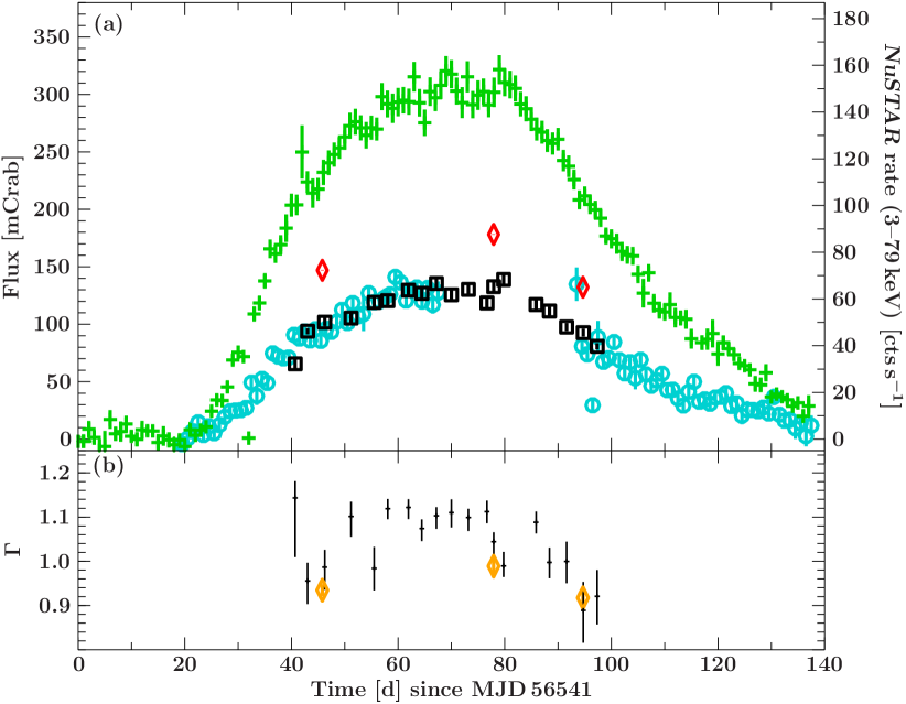
Figure 1.— (a) Lightcurve of the 2013 outburst. Data from Swift/BAT (15–50 keV, Krimm et al., 2013) are shown as green crosses, MAXI (2–20 keV) as blue circles, Swift/XRT (0.5–8 keV) as black squares and NuSTAR/FPMA (3–79 keV) as red diamonds. All data are scaled to the Crab count-rate in the respective energy band. The NuSTAR count-rate for the NuSTAR data is shown on the right-hand $y$-axis. (b) Best-fit power-law index $\Gamma$ of the Swift/XRT spectra, for details of the model see text. The orange diamonds show combined XRT and NuSTAR results.

2. Observations & data reduction

2.1. NuSTAR

NuSTAR consists of two independent grazing incidence telescopes focusing X-rays between 3–79 keV onto two Focal Plane Modules, FPMA and FPMB. We used the standard NUSTARDAS software v1.2.0 as distributed with HEASOFT 6.14 to extract spectra and lightcurves. NuSTAR spectra were used between 3–60 keV. Above 60 keV the calibration at the time of writing shows increased systematic uncertainties, and we therefore do not use those data. A detailed analysis of the high energy calibration will be presented in a forthcoming publication. The source data were extracted from a $130^{\prime\prime}$ radius circular region centered at $\alpha_{\text{J2000}}=19^{\mathrm{h}}49^{\mathrm{m}}36^{\mathrm{s}}$ and $\delta_{\text{J2000}}=+30^{\circ}12^{\prime}22^{\prime\prime}$. Background spectra were extracted from a circular region with $105^{\prime\prime}$ radius as far away from the source as possible. This formally introduces systematic uncertainties in the background estimation, but since KS 1947+300 is at least a factor of 40 brighter than the background at all energies, the influence on the source flux is negligible. Light-curves were extracted with a resolution of 1 s, the resolution corresponding to dead-time measurements in the standard operating mode.

2.2. Swift/XRT

Data from the Swift/XRT (Burrows et al., 2005) were extracted following the standard guidelines, using XSELECT to extract spectra and lightcurves and xrtmkarf to create the response files. All data were obtained in window timing mode. The source data were extracted from a circular region with a radius of 20 sky pixels ($\approx 47^{\prime\prime}$). Background spectra were extracted from the wings of the PSF using an annular region between 90 and 110 pixels radius ($212^{\prime\prime}$ and $259^{\prime\prime}$, respectively). In XRT KS 1947+300 is a factor of 50 brighter than the background at all energies, rendering small uncertainties in the background negligible. We used the XRT spectra in the energy range between 0.8–10 keV. At lower energies the windowed timing mode shows larger calibration uncertainties and we therefore decided not to use those energies.

2.3. Reduction methods

All timing information for both satellites was transferred to the solar barycenter, using the FTOOL barycorr and the DE-200 solar system ephemeris (Standish et al., 1992), and corrected for the binary motion using the ephemeris by Galloway, Morgan & Levine (2004). Timing and spectral analysis was performed using the Interactive Spectral Interpretation System (ISIS v1.6.2, Houck & Denicola, 2000). All uncertainties are given at the 90% level ($\Delta\chi^{2}=2.7$ for one parameter of interest), unless otherwise noted.

3. Phase-averaged spectroscopy

For spectral modeling, we use FPMA and FPMB spectra as well as the corresponding XRT data for each epoch, as detailed in Table 1. The X-ray continuum is very well described with a simple power-law with an exponential cutoff (model cutoffpl in XSPEC) plus a black-body. The black-body is responsible for about 50% of the flux at 2 keV and follows the overall flux evolution of the data. It likely originates from the hot-spot of the neutron star surface. The compTT model used by Naik et al. (2006) and Galloway, Morgan & Levine (2004) results in a clearly worse fit.

Naik et al. (2006) and Galloway, Morgan & Levine (2004) measured an absorption column towards the source which was lower than the maximal Galactic value along that line of sight ($\sim 9\times 10^{21}$ cm^-2, Kalberla et al., 2005). We therefore allow the absorption to vary in our model, but require it to be the same in all three observations. We describe it using an updated version of the tbabs (Wilms, Allen & McCray, 2000) model, with the corresponding abundances and cross-sections by Verner et al. (1996). Our best fit value of $8.45\pm 0.20\times 10^{21}$ cm^-2 is consistent with the 21 cm value along the line of sight and also with the ${N}_{\mathrm{H}}$ obtained from the reddening of the source ($A_{V}=3.38$; Negueruela et al., 2003) when using the calibration of Predehl & Schmitt (1995) as updated by Nowak et al. (2012).

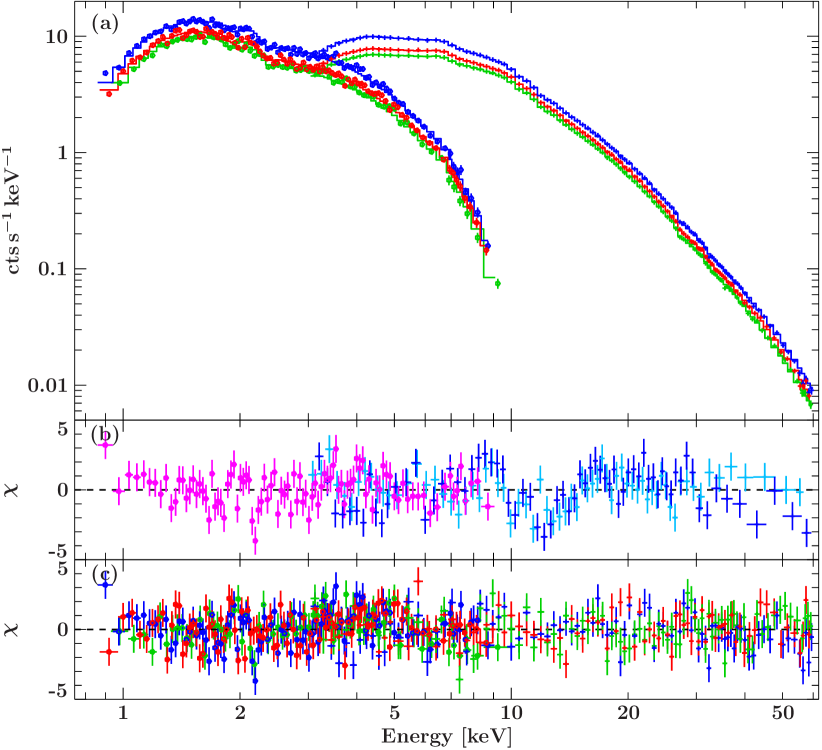
Figure 2.— (a) Data and best-fit model of Swift/XRT (circles) and NuSTAR/FPMA (crosses) for all three epochs. Observation 1 is shown in red, observation 2 in blue, and observation 3 in green. (b) Residuals of observation 2 to the best-fit model without a CRSF, rebinned for plotting purposes; Swift/XRT is shown in magenta, NuSTAR/FPMA in blue and FPMB in light blue. (c) Residuals to the best-fit model including the CRSF of all three observations in terms of $\chi$.

Adding a Gaussian $\mathrm{Fe}~{}\mathrm{K}\alpha$ line at around 6.5 keV to the continuum model we obtain a good description of the spectra, with a $\chi^{2}=3369.9$ for 3068 d.o.f. ($\chi^{2}_{\text{red}}=1.10$). The data are shown in Figure 2(a). However, close inspection of the residuals of the second observation reveals significant residuals around 13 keV (see Figure 2(b)). We therefore add a multiplicative absorption line with a Gaussian optical depth profile (model gabs in XSPEC) to the model for the second observation. This additional component improves the fit significantly to $\chi^{2}=3284.6$ for 3063 d.o.f. ($\chi^{2}_{\text{red}}=1.07$, $F$-test false positive probability $1.5\times 10^{-15}$, after Bevington & Robinson, 1992). This model is shown in Figure 2(a), the best-fit residuals in Figure 2(c), and its parameters are given in Table 2. The fluxes are given in NuSTAR/FPMA normalization and we allow for small cross-calibration differences to Swift/XRT and FPMB using the multiplicative factors $\text{C}_{\text{XRT}}$ and $\text{C}_{\text{FPMB}}$, respectively.

Table 2Fit Parameters for the Best-fit Phase-averaged Model.

Parameter	Obs. I	Obs. II	Obs. III
$N_{\text{H}}\tablenotemark{a}\tablenotemark{f}$	$0.848^{+0.024}_{-0.020}$	$0.848^{+0.024}_{-0.020}$	$0.848^{+0.024}_{-0.020}$
$\mathcal{F}_{\text{1--60\,keV}}\tablenotemark{b}$	$7.202\pm 0.027$	$9.08\pm 0.04$	$6.491\pm 0.021$
${L}_{\text{1--60\,keV}}\tablenotemark{c}$	$8.62\pm 0.03$	$10.87\pm 0.05$	$7.768\pm 0.024$
$\Gamma$	$0.928\pm 0.014$	$0.982^{+0.022}_{-0.015}$	$0.927^{+0.014}_{-0.012}$
$E_{\text{cut}}(\text{keV})$	$22.5^{+0.5}_{-0.4}$	$24.2^{+0.6}_{-0.5}$	$22.13^{+0.45}_{-0.24}$
$E_{\text{CRSF}}(\text{keV})\tablenotemark{f}$	$12.2^{+0.5}_{-0.7}$	$12.2^{+0.5}_{-0.7}$	$12.2^{+0.5}_{-0.7}$
$\sigma_{\text{CRSF}}(\text{keV})\tablenotemark{f}$	$2.5^{+1.3}_{-0.6}$	$2.5^{+1.3}_{-0.6}$	$2.5^{+1.3}_{-0.6}$
$d_{\text{CSRF}}(\text{keV})$	$0.00^{+0.04}_{-0.05}$	$0.16^{+0.15}_{-0.05}$	$-0.05^{+0.04}_{-0.10}$
$A_{\text{BB}}\tablenotemark{c}$	$4.12^{+0.21}_{-0.20}$	$5.73^{+0.28}_{-0.52}$	$3.45^{+0.19}_{-0.18}$
$kT(\text{keV})$	$0.663^{+0.017}_{-0.018}$	$0.745^{+0.017}_{-0.026}$	$0.636^{+0.023}_{-0.016}$
$A(\text{Fe\,K}\alpha)\tablenotemark{d}$	$1.78^{+0.20}_{-0.19}$	$2.28^{+0.22}_{-0.25}$	$1.20^{+0.16}_{-0.12}$
$E(\text{Fe\,K}\alpha)(\text{keV})\tablenotemark{e}$	$6.575^{+0.030}_{-0.032}$	$6.563^{+0.031}_{-0.028}$	$6.539^{+0.029}_{-0.031}$
$\sigma(\text{Fe\,K}\alpha)(\text{keV})\tablenotemark{e}$	$0.29\pm 0.05$	$0.31\pm 0.04$	$0.25\pm 0.04$
$\text{C}_{\text{XRT}}$	$0.967\pm 0.014$	$0.966^{+0.012}_{-0.015}$	$0.982^{+0.017}_{-0.015}$
$\text{C}_{\text{FPMB}}$	$1.0207\pm 0.0023$	$1.0308\pm 0.0021$	$1.0232\pm 0.0021$

We search for similar absorption lines in the spectra of the other two observations. For that we require the energy and width of the gabs component to be the same in all observations and allow only the depth to vary in a simultaneous fit to all three data-sets. In both other data-sets the line is not significantly detected (Table 2). The 90% uncertainties are clearly below the depth of the line during observation 2, indicating a physical change in the source spectrum over the outburst.

3.1. Time-resolved spectral analysis

To study the evolution of the spectrum over the outburst we use all available Swift/XRT data between MJD 56581–56639, and describe them with the same cutoffpl plus bbody model as the time-averaged spectra. We fix the cutoff-energy at 23.2 keV, the average value in the NuSTAR data and the absorption column to $8.45\times 10^{21}$ cm^-2, since the Galactic absorption column should not vary.

We find a strong degeneracy between the power-law slope and the black-body temperature due to the limited energy range covered by Swift/XRT. From the simultaneous NuSTAR and Swift/XRT spectra it becomes clear, however, that an almost linear correlation between the black-body temperature and the unabsorbed 3–10 keV flux is present,

$$kT_{\text{bbody}}=m\times\mathcal{F}_{\text{3--10\,keV}}\text{,}$$ (2)

where $kT_{\text{bbody}}$ is measured in keV and $\mathcal{F}_{\text{3--10\,keV}}$ in keV s^-1 cm^-2. In the simultaneous fits we find $m=0.576\pm 0.010$ s cm². We use this correlation to tie the black-body temperature to the X-ray flux in the time-resolved XRT spectra and consequently replace the degeneracy with an empirically motivated correlation.

The remaining free parameters in the model are the photon-index of the power-law, the 3–10 keV flux and the relative normalization of the black-body component. The latter does not show significant changes with time. The model describes all 19 XRT spectra relatively well, with an average $\chi^{2}_{\text{red}}$ =1.05 for 429 d.o.f.

As shown in Figure 1(b), the photon-index is highly variable and seems to soften with increased X-ray flux. This correlation is marginally significant at a bit above the 1$\sigma$ level, with Spearman’s rank correlation coefficient $\rho=0.31$. It also becomes clear that all three NuSTAR observations were performed during phases with relatively hard spectra. Tsygankov & Lutovinov (2005) found a similar correlation between then photon index and the X-ray luminosity in the harder RXTE energy band (3–100 keV).

4. Phase-resolved spectroscopy

To investigate changes with viewing angle onto the neutron star we split each NuSTAR data set into 20 phase bins. For this analysis we did not use the Swift/XRT data, as their short exposure does not allow us to split them up further. We define the phase bins to stretch over intervals of similar flux and hardness ratio, see Figure 3. The pulse profile changes drastically with energy, developing from one broad pulse to a double-peaked profile, with a narrow primary and broader secondary peak above $\sim$25 keV (see also Naik et al., 2006).

To define the phase bins individually for each observation, we first measure the local pulse period by folding the cleaned NuSTAR event list on trial periods around the expected period of 18.8 s, following the description given by Leahy & Scott (1998). The uncertainties are estimated by phase-connecting pulse-profiles from the beginning and end of each observation. We do not allow for a change in the pulse period during one observation, but the error introduced is below the precision needed for the analysis presented here. The measured periods show a continuous spin-up over the duration of the outburst (see Table 1), in agreement with the Swift/XRT snap-shots and the Fermi/GBM pulsar monitoring (Finger et al., 2009).

To describe the phase-resolved spectra we use the same model as for the phase-averaged spectrum, but fix the line energies and widths of the CRSF and the $\mathrm{Fe}~{}\mathrm{K}\alpha$ line as well as the temperature of the black-body due to the reduced statistical quality of the spectra. This model results in a very good description of the data in all phase bins, with an average $\chi^{2}_{\text{red}}=1.02$ for 345 d.o.f.

Figure 3 shows the continuum parameters only for the second observation, since it provides the best statistics, but the other two observations show very similar behavior. Both the photon-index $\Gamma$ and the folding energy $E_{\text{fold}}$ show a very strong dependence on phase, confirming the results by Naik et al. (2006) at a much higher resolution in phase space (Figure 3 left, (c) and (d)). Between phase 0.1–0.2 we observe a strong increase in $\Gamma$ and $E_{\text{fold}}$, coincident with the small dip between the narrow first peak and the broad main peak.

The strength of the CRSF shows a very interesting behavior with pulse phase, as shown for all observations in Figure 3, right panel. As expected from the phase-averaged spectra, the line is clearly strongest in observation 2, being detectable over a wide phase-range between phases 0.6–1.3. During the main peak of the pulse-profile the line strength drops to 0. In observation 1 the line is also significantly detected in absorption between phases 0.9–1.1. Around phase 0.3 there are low significance indications that the line is instead visible in emission. In observation 3 the line strength is scattering around 0, only one phase bin around phase 1.0 shows an absorption line clearly above the 95% limit.

In the phase-resolved spectra we allow the iron line normalization and the black-body normalization to vary to obtain a statistically acceptable fit (not shown in Figure 3). We carefully checked that any variation in these parameters does not influence the strength of the CRSF. While the iron line shows the largest equivalent width during the minimum of the pulse profile, i.e., at the same phases where the CRSF is most prominent, it does not influence the spectral shape at the CRSF energy. The black-body did not vary significantly over the pulse phase.

To investigate the energy dependence of the CRSF with pulse-phase, we extracted spectra from observation 2 using seven, wider phase bins to increase the S/N. For these spectra we also allow the iron line energy and width, as well as the blackbody temperature to vary. We keep the width of the CRSF fixed to the best phase-averaged value, as it otherwise became unconstrained during the fits. As can be seen in Figure 3, right (a) we do not detect a significant variation of the line energy with pulse phase. Between phases 0.4–0.6 we again detected no significant line, resulting in an unconstrained energy.

Besides changes with pulse-phase, changes of the line energy with luminosity are quite common (see, e.g. Caballero et al., 2007; Tsygankov, Lutovinov & Serber, 2010; Fürst et al., 2014, among others). To search for such a luminosity dependence between observations, we extract spectra for each observation of those phases, in which the line was significantly detected in observation 2. This approach allows to obtain the most significant line and therefore most precise energy measurement, as indicated by the blue data points in Figure 3. We describe the spectra with the same model as for the seven wide phase bins described above. We do not detect a significant change of the line energy, with the measured values being $12.5\pm 0.7$ keV, $12.3\pm 0.5$ keV, and $12.2\pm 0.9$ keV for observation 1, 2, and 3 respectively.

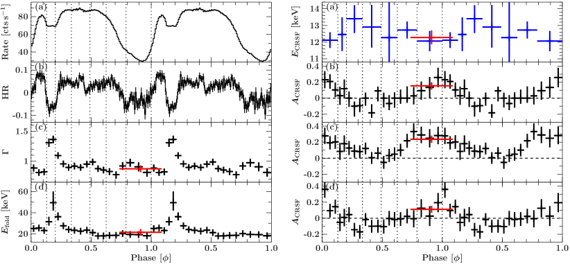
Figure 3.— Results of the phase resolved spectroscopy. The left panel shows for observation 2 the (a) pulse-profile between 3–79 keV, (b) hardness ratio $(H-S)/(H+S)$ between the energy bands $S$=4.5–6 keV and $H$=10–15 keV. The dotted lines indicate the seven, wider phase bins used to measure the CRSF energy. The photon-index $\Gamma$ and the folding energy are shown in panels (c) and (d), respectively. The right panel shows the parameters of the CRSF: (a) line energy for the second observation, (b), (c), and (d) line strength for the first, second, and third observation, respectively. The red data-points show the results of the phase bin covering the phases with the most significant CRSF in observation 2; see text for details. The pulse is repeated once for clarity.

5. Summary & Discussion

We have presented a spectral analysis of three NuSTAR observations of the Be-X-ray binary KS 1947+300 with simultaneous Swift/XRT data, taken during its large 2013/2014 outburst. The broad spectral coverage provided by the combination of these two instruments allowed us to discover a CRSF absorption feature around 12.5 keV. The feature was significantly detected in the phase-averaged spectrum of the brightest observation, and during the broad pulse minimum in phase-resolved spectroscopy in all observations. During the pulse maximum the feature is not seen significantly, either in absorption or emission.

The line energy and width is similar to the lines detected in 4U 0115+63 and Swift J1626.6$-$5156 (White, Swank & Holt, 1983; DeCesar et al., 2013). We deduce a surface magnetic field of $\sim 1.1\times 10^{12}(1+z)$ G, assuming that the line is the fundamental line. Here $z$ is the gravitational redshift, defined by

$$(1+z)^{-1}=\sqrt{1-\frac{2GM}{Rc^{2}}}.$$ (3)

For typical neutron star parameters, $z\approx 0.3$ if the line-forming region is close to the surface. This magnetic field strength puts KS 1947+300 at the lower end of known cyclotron lines sources (cf. Caballero et al., 2007).

During the broad minimum phase of the pulse profile, we detect the CRSF in all three observations. The luminosity near $10^{38}$ erg s^-1 puts KS 1947+300 clearly in the super-critical accretion regime, where the radiation pressure is strong enough to decelerate the in-falling matter before the neutron star surface via a radiation-dominated shock (Becker et al., 2012). In this regime, a negative correlation between the CRSF energy and luminosity is expected (Becker et al., 2012), as observed, for example, in V 0332+53 (Tsygankov, Lutovinov & Serber, 2010). If the correlation were of a similar strength as observed in V 0332+53 we would not have detected it due to the very small range of luminosities sampled.

The time-resolved Swift/XRT spectra show a strongly variable photon-index $\Gamma$ over the outburst, with changes of 10% or more within 3 days and softening with increasing X-ray flux. This softening agrees with the expected behavior in the supercritical accretion regime, as shown by Klochkov et al. (2011) for various other sources. However, because we restricted the model to describe basically all changes in spectral hardness in the photon-index, it is probable that the true physical changes are more complex than a variable photon-index, e.g., the black-body temperature might vary independently of the X-ray flux. Nonetheless, intrinsic source variability must be present.

We clearly detect a $\mathrm{Fe}~{}\mathrm{K}\alpha$ line in all data sets, with an energy significantly above the line energy for neutral iron (see Table 2) and broadened in excess of the energy resolution of NuSTAR. While Doppler-broadening could be responsible for part of the observed width, the increased energy indicates that the fluorescence region is slightly ionized and the observed broadening originates from a blend of $\mathrm{Fe}~{}\mathrm{K}\alpha$ at different low ionization states. The data do not allow us to disentangle different lines from one single broad line.

References

- Becker et al. (2012) Becker, P. A., et al., 2012, A&A, 544, A123
- Bevington & Robinson (1992) Bevington, P. R., & Robinson, D. K., 1992, Data reduction and error analysis for the physical sciences, The McGraw-Hill Companies, Inc.), 2 edition
- Borozdin et al. (1990) Borozdin, K., et al., 1990, Soviet Astronomy Letters, 16, 345
- Burrows et al. (2005) Burrows, D. N., et al., 2005, Space Sci. Rev., 120, 165
- Caballero et al. (2007) Caballero, I., et al., 2007, A&A, 465, L21
- Chakrabarty et al. (1995) Chakrabarty, D., Koh, T., Bildsten, L., Prince, T. A., Finger, M. H., Wilson, R. B., Pendleton, G. N., & Rubin, B. C., 1995, ApJ, 446, 826
- DeCesar et al. (2013) DeCesar, M. E., Boyd, P. T., Pottschmidt, K., Wilms, J., Suchy, S., & Miller, M. C., 2013, ApJ, 762, 61
- Finger et al. (2009) Finger, M. H., et al., 2009, in Proc. of the 2009 Fermi Symposium, eConf Proceedings C091122, arXiv:0912.3847)
- Finger et al. (1994) Finger, M. H., Stollberg, M., Pendleton, G. N., Wilson, R. B., Chakrabarty, D., Chiu, J., & Prince, T. A., 1994, IAU Circ., 5977
- Fürst et al. (2014) Fürst, F., et al., 2014, ApJ, 780, 133
- Galloway, Morgan & Levine (2004) Galloway, D. K., Morgan, E. H., & Levine, A. M., 2004, ApJ, 613, 1164
- Harrison et al. (2013) Harrison, F. A., et al., 2013, ApJ, 770, 103
- Houck & Denicola (2000) Houck, J. C., & Denicola, L. A., 2000, in Astronomical Data Analysis Software and Systems IX, ed. N. Manset, C. Veillet, D. Crabtree, Vol. 216, (San Francisco: Astron. Soc. Pac.), 591
- Hua & Titarchuk (1995) Hua, X., & Titarchuk, L., 1995, ApJ, 449, 188
- Iwakiri et al. (2012) Iwakiri, W. B., et al., 2012, ApJ, 751, 35
- Kalberla et al. (2005) Kalberla, P. M. W., Burton, W. B., Hartmann, D., Arnal, E. M., Bajaja, E., Morras, R., & Pöppel, W. G. L., 2005, A&A, 440, 775
- Kawagoe et al. (2013) Kawagoe, A., et al., 2013, The Astronomer’s Telegram, 5438
- Kennea et al. (2013) Kennea, J. A., Evans, P. A., Krimm, H. A., Romano, P., Mangano, V., Curran, P., Yamaoka, K., & Negoro, H., 2013, The Astronomer’s Telegram, 5441
- Klochkov et al. (2011) Klochkov, D., Staubert, R., Santangelo, A., Rothschild, R. E., & Ferrigno, C., 2011, A&A, 532, A126
- Krimm et al. (2013) Krimm, H. A., et al., 2013, ApJS, 209, 14
- Leahy & Scott (1998) Leahy, D. A., & Scott, D. M., 1998, ApJ, 503, L63
- Matsuoka et al. (2009) Matsuoka, M., et al., 2009, PASJ, 61, 999
- Naik et al. (2006) Naik, S., Callanan, P. J., Paul, B., & Dotani, T., 2006, ApJ, 647, 1293
- Negueruela et al. (2003) Negueruela, I., Israel, G. L., Marco, A., Norton, A. J., & Speziali, R., 2003, A&A, 397, 739
- Nowak et al. (2012) Nowak, M. A., et al., 2012, ApJ, 759, 95
- Predehl & Schmitt (1995) Predehl, P., & Schmitt, J. H. M. M., 1995, A&A, 293, 889
- Schönherr et al. (2007) Schönherr, G., Wilms, J., Kretschmar, P., Kreykenbohm, I., Santangelo, A., Rothschild, R. E., Coburn, W., & Staubert, R., 2007, A&A, 472, 353
- Standish et al. (1992) Standish, E. M., Newhall, X. X., Williams, J. G., & Yeomans, D. K., 1992, in Explanatory Supplement to the Astronomical Almanac, ed. P. K. Seidelmann, 279, (Mill Valley: University Science Books)
- Swank & Morgan (2000) Swank, J., & Morgan, E., 2000, IAU Circ., 7531, 4
- Titarchuk (1994) Titarchuk, L., 1994, ApJ, 434, 570
- Tsygankov & Lutovinov (2005) Tsygankov, S. S., & Lutovinov, A. A., 2005, Astronomy Letters, 31, 88
- Tsygankov, Lutovinov & Serber (2010) Tsygankov, S. S., Lutovinov, A. A., & Serber, A. V., 2010, MNRAS, 401, 1628
- Verner et al. (1996) Verner, D. A., Ferland, G. J., Korista, K. T., & Yakovlev, D. G., 1996, ApJ, 465, 487
- White, Swank & Holt (1983) White, N. E., Swank, J. H., & Holt, S. S., 1983, ApJ, 270, 711
- Wilms, Allen & McCray (2000) Wilms, J., Allen, A., & McCray, R., 2000, ApJ, 542, 914