Multiwavelength Observations of the Candidate Disintegrating sub-Mercury KIC 12557548b

Abstract

We present multiwavelength photometry, high angular resolution imaging, and radial velocities, of the unique and confounding disintegrating low-mass planet candidate KIC 12557548b. Our high angular resolution imaging, which includes spacebased HST/WFC3 observations in the optical ($\sim$0.53 $\mu m$ and $\sim$0.77 $\mu m$), and groundbased Keck/NIRC2 observations in K’-band ($\sim$2.12 $\mu m$), allow us to rule-out background and foreground candidates at angular separations greater than 0.2″ that are bright enough to be responsible for the transits we associate with KIC 12557548. Our radial velocity limit from Keck/HIRES allows us to rule-out bound, low-mass stellar companions ($\sim$0.2 M_⊙) to KIC 12557548 on orbits less than 10 years, as well as placing an upper-limit on the mass of the candidate planet of 1.2 Jupiter masses; therefore, the combination of our radial velocities, high angular-resolution imaging, and photometry are able to rule-out most false positive interpretations of the transits. Our precise multiwavelength photometry includes two simultaneous detections of the transit of KIC 12557548b using CFHT/WIRCam at 2.15 $\mu m$ and the Kepler space telescope at 0.6 $\mu m$, as well as simultaneous null-detections of the transit by Kepler and HST/WFC3 at 1.4 $\mu m$. Our simultaneous HST/WFC3 and Kepler null-detections, provide no evidence for radically different transit depths at these wavelengths. Our simultaneous CFHT/WIRCam detections in the near-infrared and with Kepler in the optical reveal very similar transit depths (the average ratio of the transit depths at $\sim$2.15 $\mu m$ compared to $\sim$0.6 $\mu m$ is: 1.02 $\pm$ 0.20). This suggests that if the transits we observe are due to scattering from single-size particles streaming from the planet in a comet-like tail, then the particles must be $\sim$0.5 microns in radius or larger, which would favour that KIC 12557548b is a sub-Mercury, rather than super-Mercury, mass planet.

1. Introduction

Rappaport et al. (2012) presented intriguing, perplexing and downright peculiar Kepler observations of the K-dwarf star KIC 12557548. The Kepler space telescope’s (Borucki et al., 2009) observations of this star displayed repeating dips every $\sim$15.7 hours that varied in depth from a maximum of $\sim$1.3% of the stellar flux to a minimum of $\sim$0.2% or less without a discernible rhyme or reason to explain the depth variations. In addition, the occultations were not the iconic transit-like shape we have come to expect from extrasolar planets or binary stars, but exhibited an obvious ingress/egress asymmetry, with a sharp ingress followed by a longer, more gradual egress. A non-detection of ellipsoidal light variations allowed an upper-limit on the mass of the occulting object to be set at 3 Jupiter masses, and thus prompted the question of what was causing this odd photometry? The answer the authors proposed was that the peculiar Kepler observations of KIC 12557548 (hereafter KIC 1255) are due to a gradually disintegrating low mass (super-Mercury) planet, KIC 12557548b (hereafter KIC 1255b). The thought process is that this putative planet, with its extremely short orbital period, is being roasted by its host star, and is throwing off material in fits and starts; at each passage in front of its parent star, the different amount of material being discarded by the planet leads to differences in the resulting optical depth, thus explaining the obvious transit depth variations. The clear ingress/egress asymmetry of the transit is then due to the fact that the material is streaming behind the planet, forming a long comet-like tail that obscures the star for a larger fraction of the orbit.

Naturally, observations as odd as those presented by Rappaport et al. (2012) and an explanation as exotic as a disintegrating super-Mercury, invited a great deal of skepticism from the astronomical community. Alternative theories that have been discussed to explain the observed photometry include: (i) a bizarre Kepler photometric artifact; (ii) a background blended eclipsing binary; (iii) an exotically chaotic triple; or (iv) a binary that is orbiting KIC 12557548 wherein one member of the binary system is a white dwarf fed by an accretion disk (Rappaport et al., 2012).

Inspired by the Rappaport et al. (2012) result there have been a number of modelling efforts to interpret the bizarre Kepler observations that seem to reinforce the possibility that the photometry of KIC 1255 is caused by scattering off material streaming from a disintegrating low-mass planet. Dust scattering models confirm the viability of the disintegrating planet scenario featuring a comet-like tail trailing the planet, composed of sub-micron sized grains (Brogi et al., 2012), or up to one micron (0.1 - 1.0 $\mu m$) sized grains (Budaj, 2013). These efforts suggest that the minute brightening just prior to transit can be readily explained by enhanced forward scattering from this dust cloud, while the ingress/egress asymmetry can be explained by a comet-like dust tail that has a particle density or size distribution that decreases with distance from the planet. The richness of the Kepler data on KIC 1255b have led to suggestions of evolution of the cometary tail (Budaj, 2013), and that the comet is best explained by a two component model, with a dense coma and inner-tail and a diffuse outer tail (Budaj, 2013; van Werkhoven et al., 2013). Another effort by Kawahara et al. (2013) suggests that the observed transit depth variability may correlate with the stellar rotation period, and thus the presumed variable mass loss rate of the planet may be a byproduct of the stellar activity, specifically ultraviolet and X-ray radiation. Perez-Becker & Chiang (2013) argue from the results of a hydrodynamical wind model, that we may be observing the final death-throes of a planet catastrophically evaporating, and that KIC 1255b may range in mass from 0.02 - 0.07 $M_{\oplus}$ (less than twice that of the Moon, to greater than Mercury), although for most solutions the mass of KIC 1255b is less than that of Mercury. We note that subsequent to the submission of this work, there has been an announcement of a second low-mass planet candidate, possibly hosting a comet-like tail (Rappaport et al., 2014).

One proposed method for elucidating the unknown nature of the material that is supposedly occulting KIC 1255, is multiwavelength simultaneous observations of the transit of the object. As the efficiency of scattering diminishes for wavelengths longer than the approximate particle size (Hansen & Travis, 1974), and given the inference of sub-micron size grains in the dust tail of this object (Brogi et al., 2012; Budaj, 2013), one might expect that infrared and near-infrared photometry of the transit of KIC 1255b would display significantly smaller depths than those displayed in the optical. Determining that the transit depth of KIC 1255b is wavelength dependent, with smaller depths in the near-infrared than the optical, would therefore strongly favour the explanation of scattering from a dust tail with sub-micron sized particles.

Here we present an assortment of different observations of KIC 1255 that were obtained in order to either bolster or rule-out the disintegrating low-mass planet scenario. In addition to the Kepler photometry that we analyze here, these various observational data include: (i) two Canada-France-Hawaii Telescope/Wide-field InfraRed Camera (CFHT/WIRCam) Ks-band ($\sim$2.15 micron) photometric detections of the KIC 1255b transit with simultaneous Kepler photometric detections, (ii) simultaneous photometric non-detections of the KIC 1255b transit with the Hubble Space Telescope Wide Field Camera 3 (HST/WFC3) F140W and Kepler photometry, (iii) HST/WFC3 high-angular resolution imaging of KIC 1255 in the F555W ($\lambda$$\sim$0.531 $\mu m$), and F775W ($\lambda$$\sim$0.765 $\mu m$) bands, (iv) Keck/NIRC2 ground-based Adaptive Optics (tip/tilt only) high-angular resolution imaging of KIC 1255 in the K’-band ($\lambda\sim$2.124 $\mu m$), and (v) and Keck/HIRES radial velocity observations of KIC 1255. The high angular resolution imaging observations allow us to rule-out nearby background/foreground companions as close as 0.2″ to KIC 1255. Our KECK/HIRES radial velocity observations allow us to rule-out low-mass stellar companions ($\sim$ 0.2 M_⊙) for orbital periods $\lesssim 10$ years. This significantly reduces the parameter space for nearby companions to KIC 1255, and therefore reduces the odds that the unique Kepler photometry that Rappaport et al. (2012) reported is due to a binary or higher-order multiple, masquerading as a planetary false positive. Our simultaneous Kepler and near-infrared detections of the transit of KIC 1255b appear to report similar depths; as a result, if the source of the photometry we observe is a dust tail trailing a disintegrating planet composed of single-sized particles, then the particles are at least $\sim$0.5 microns in radius. Particles this large can likely only be lofted from a low-mass planet, suggesting that KIC 1255b might best be described as a sub-Mercury mass planet.

2. Observations and Analysis

2.1. Kepler photometry

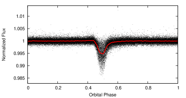
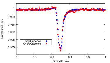
Figure 1.— Top panel: Kepler long cadence photometry (black points) of KIC 1255 phased to the orbital period of the candidate planet ($\sim$15.685 hours). The red line is the binned mean of the orbital phase-folded light curve. Bottom panel: The binned mean of the phase-folded light curve (every $\phi$=0.005 in phase) of the short cadence (red circles) and long cadence (blue squares) photometry.

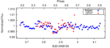
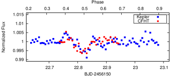
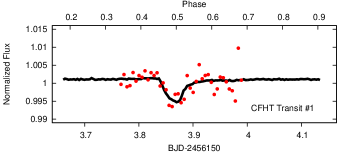
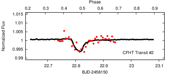
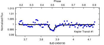
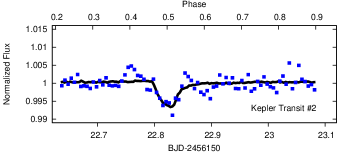
Figure 2.— CFHT/WIRCam Ks-band photometry (red circles) and Kepler photometry (blue squares) of the transit of KIC 1255b obtained on the nights of 2012 August 13 (left panels) and 2012 September 1 (right panels; Hawaiian Standard Time). Both sets of data are binned every 8 minutes. The black lines in the bottom two sets of panels indicate the best-fit transit model for each set of data; the transit model is a scaled version of the mean of the short-cadence, phase-folded Kepler light curve ($g(t)$; see $\S$2.1).

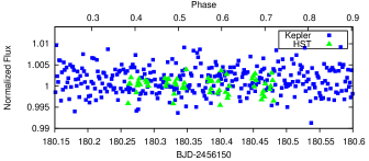
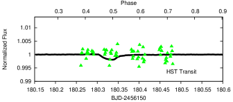
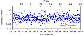
Figure 3.— HST F140W filter photometry (1.4$\mu m$; green triangles) and Kepler photometry (blue squares) of the transit of KIC 1255b obtained on 2013 February 6 (UTC). The Kepler and the HST data are binned every 2 minutes. The black lines in the bottom two panels indicate the 3$\sigma$ upper limit on the transit depth obtained by scaling the mean of the short-cadence, phase-folded Kepler light curve ($g(t)$; see $\S$2.1).

We start by presenting an analysis of the Kepler data of KIC 1255. We analyze all the long cadence (quarters 1-16 at the time of writing; 29.4 minute sampling) and short cadence (quarters 13-16; 58.8 second sampling) Simple Aperture Photomery (SAP) of this star. KIC 1255 displays obvious rotational modulation with a period of $\sim$22.9 $d$ that varies between 1-4% of the observed stellar flux; we remove this modulation by employing a cubic spline. To ensure that KIC 1255b’s variable and asymmetric transit depth in no way impacts our starspot removal technique, we cut out all data in the transit before calculating our cubic spline; that is, we phase the data to the orbital period of the putative planet (where phase, $\phi$=0.5 denotes the midpoint of the transit), and cut out all data between phases $\phi$=0.4-0.7, and then bin the data every $\sim$10 hours. After calculating the cubic spline on the binned Kepler data with the transits removed, we apply the cubic spline to all the unbinned Kepler data and apply a 10$\sigma$ cut to remove outliers; we thus produce a light curve of KIC 1255 with the obvious rotational modulation removed. The spot-corrected, phase-folded, long cadence light curve of KIC 1255 is presented in the top panel of Figure 1; the short-cadence data are similar, but have much higher scatter per point. We present the phase-folded, binned mean of the long and short cadence data in the bottom panel of Figure 1. We note that the short cadence data display a marginally narrower transit, and appears to have an extra, brief, enhanced decrement in flux following the transit (i.e., near phase $\phi$=0.65) that is not visible in the long cadence photometry

To compare the Kepler photometry to our CFHT groundbased ($\S$2.2) and HST spacebased ($\S$2.3.1) photometry, we also present the Kepler SAP photometry, without the spline-correction. Given the asymmetric transit profile and varying transit depth displayed in the Kepler photometry, we choose to fit our individual Kepler transits (and the simultaneous CFHT and HST photometry) by scaling the mean transit profile of the short cadence Kepler photometry by a multiplicative factor, $A$. Therefore the function we use to fit our data, $g(t)$ is compared to the mean of the phase-folded short cadence photometry, $f(t)$ (shown in the bottom panel of Figure 1), by:

$$g(t)=1+A\,[f(t-t_{transit})-1]+y_{o}$$ (1)

where $y_{o}$ is simply a vertical offset, and $t_{transit}$ is the mid-transit time (defined as the minimum of the phase-folded mean of the short cadence photometry, at phase $\phi$=0.5). We note that a value of $A$ = 1 corresponds to a KIC 1255b transit depth of 0.55% of the stellar flux, as shown in the bottom panel of Figure 1. We note that by multiplying our phase-folded mean by $A$ we are scaling up or down the size of the apparent forward-scattering peak, as well as the depth of the transit. To fit our Kepler transits, as well as the CFHT and HST transits that follow, we employ Markov Chain Monte Carlo (MCMC) techniques (as described for our purposes in Croll 2006). In Figures 2 and 3 we present the SAP short cadence Kepler photometry of KIC 1255b that was obtained simultaneously with the CFHT and HST photometry, as well as the best-fit scaled profile, $g(t)$, of the mean short-cadence Kepler profile, $f(t)$. We assume an error on the Kepler data for our MCMC fitting based on the RMS of the residuals to the best-fit model. The associated best-fit parameters are presented in Table 1.

2.2. CFHT/WIRCam photometry

Figure 4.— The root-mean-square of our photometry after the subtraction of our best-fit (solid line) for our CFHT/WIRCam Ks-band photometry of our first-transit (left), and our second-transit (right). The dashed line in each panel displays the one over the square-root of the bin-size expectation for Gaussian noise.

We obtained two Ks-band ($\sim$2.15 micron) WIRCam (Puget et al., 2004) photometric data-sets of the transit of KIC 1255 ($K$$\sim$13.3). Data-sets were obtained on the evenings of 2012 August 13 and 2012 September 1 (Hawaiian Standard Time). The observations lasted for $\sim$6.5 hours and $\sim$5 hours, respectively. High wind impacted the image quality for the first set of observations (2012 August 13); the second set of observations were of photometric quality throughout the night (2012 September 1). Reduction of the data and aperture photometry was performed as detailed in Croll et al. (2010a, b). Although WIRCam offers a 21′$\times$21′ field-of-view, we only utilize reference stars from the same detector as our target, therefore resulting in a 10′$\times$10′ field-of-view. We employ a range of aperture radii for our CFHT photometry (as discussed below in $\S$2.2.1), and subtracted the sky in all cases using an annulus with an inner and outer radius of 14 and 20 pixels, respectively. To determine the fractional contribution of the square pixels at the edge of the circular aperture we multiply the flux of these pixels by the fraction of the pixels that falls within our circular aperture; we determine this fractional contribution using the GSFC Astronomy Library IDL procedure pixwt.pro. The exposure times were 25 seconds, with an overhead for read-out and saving exposures of 7.38 seconds, resulting in an overall duty-cycle of $\sim$76%. The telescope was defocused to 0.9 mm for both observations. In both cases at the conclusion of the observations the airmass increased to beyond 2.0; we noticed reduced precision in the resulting light curves once the airmass rose above a value of 1.6. As a result, we exclude all data with an airmass greater than this latter value in the following analysis. Our CFHT photometry is presented in the middle panels of Figure 2, using aperture radii of 7 and 9 pixels for our first and second CFHT transits, respectively. After the subtraction of our best-fit models, we achieve an RMS precision of 7.1$\times$$10^{-3}$ and 6.5$\times$$10^{-3}$ per exposure for our first and second transit, respectively. This compares to the expected photon noise limit of 1.15$\times$$10^{-3}$ per exposure, or 3.52$\times$$10^{-3}$ once other noise sources (read-noise, dark and sky-noise, where the sky is the dominant component) are taken into account. We compare our photometric precision to the Gaussian noise expectation of one over the square-root of the bin-size in Figure 4. Both data-sets scale down above this limit, indicative of correlated noise; some of this correlated noise is likely astrophysical as the Kepler data display obvious modulation, likely due to granulation or evolution of starspots, plages, etc., that appears to be partially replicated in the CFHT near-infrared photometry.

We fit our CFHT Transits with the scaled-version of the short-cadence, phase-folded Kepler light curve ($g(t)$; $\S$2.1). The best-fit transits are displayed in Figure 2, and the associated transit depths, $A$, compared to the mean Kepler transit depth, are given in Table 1.

We also note that as our CFHT photometry has slightly superior angular resolution than the coarse Kepler pixels, our CFHT photometry allows us to place a limit on the angular separation of the transiting object from KIC 1255. Assuming the transits we observe in our CFHT photometry are due to the same object causing the transits we observe in the Kepler data, and given the 7-9 pixel aperture we use here and WIRCam’s 0.3″pixel-scale, the object causing the transits we associate with the candidate planet KIC 1255b cannot be due to a companion more than $\sim$2″away from KIC 1255.

2.2.1 Correlations with Aperture size and Number of Reference Stars

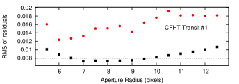
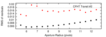
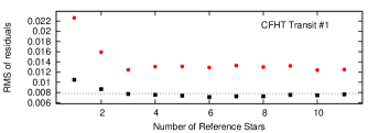
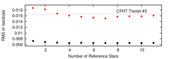
Figure 5.— Top panels: The RMS of the residuals from the best-fit MCMC fit (black squares), and the residuals multiplied by the relevant $\beta$ factor (red circles) for each of the various aperture sizes (using the best 7 reference stars), for our first (left) and second (right) transit CFHT/WIRCam Ks-band transit. Second from top set of panels: The associated measured MCMC transit depths, $A$. The bottom four panels are the same as the top four, except they display the RMS and $A$ values for the different number of reference stars for our first transit (left; 7.0-pixel aperture radius) and our second transit (right; 9.0-pixel aperture radius). We average over all $A$ values for aperture radii and number of reference stars with RMS values (black points) below the black dotted line for the first CFHT transit (left panel); for the second transit (right panel) we average all $A$ values with RMS$\times$$\beta$ values (red points) below the black dotted line.

We also search for correlations in our CFHT photometry between the measured transit depth and our choice of aperture size, and the choice of the number of reference stars. With our other CFHT photometry of hot Jupiters (Croll et al. in prep.), in some cases we noticed moderate correlations between the secondary eclipse or primary transit depths and the aperture radius chosen for aperture photometry, or the choice of the ensemble of reference stars we use to correct our photometry. Despite these changes in the transit/eclipse depth, the differences in the RMS of the residuals to the best-fit model were often negligible. Therefore we were confronted with a range of seemingly equally good fits to the data, where, troublingly, the parameter of interest, the transit/eclipse depth, varied significantly. As a result, rather than quoting just the best-fit of a single aperture and reference star combination, we quote the weighted mean of a number of aperture photometry and reference star combinations, and scale up the associated error to take into account these correlations.

To decide the best reference star and aperture radius combination, we generally use the RMS of the residuals multiplied by $\beta$, which parameterizes the amount of time-correlated red-noise in the photometry. $\beta$ is defined, employing the methods of Winn et al. (2008), as the factor by which the residuals scale above the Gaussian noise expectation (see Figure 4); to determine this number we take the average of bin sizes between 10 and 80 binned points. In general, we have noticed that the RMS$\times$$\beta$ of the residuals is a superior metric to determine the best aperture size/reference star combination than simply the RMS; for our near-infrared photometry, which generally suffers from high sky background compared to the optical, the RMS of the residuals generally reaches a minimum for relatively small apertures, as one is able to reduce the impact of the high sky background. However, these small apertures often suffer from time-correlated red-noise (high $\beta$s), as during moments of poor seeing or tracking errors, a small fraction of the light falls outside these small apertures. A small complication for our CFHT/WIRCam Ks-band photometry of KIC 1255, however, is that, as noted above, we believe that some of the correlated red-noise we observe is genuine, as it reproduces, in part, the short-term variations visible in the Kepler optical photometry. Therefore we qualitatively noticed that the most useful metrics were the RMS of the residuals for the first CFHT/WIRCam transit, and the RMS of the residuals multiplied by $\beta$ for the second CFHT/WIRCam transit; this combination produced the most satisfactory results. For this reason, we used these two different metrics to determine the best reference star ensemble and aperture size combination below.

In Figure 5 we present the correlations with aperture radius and the number of stars in our reference star ensemble for both our first and second CFHT transit of KIC 1255b. For both cases we display the variation in RMS, and the variation in RMS multiplied by $\beta$, for a variety of aperture radii and different number of reference stars in the ensemble, as well as the associated variation in the associated KIC 1255b transit depths, as parameterized by $A$. In the top set of panels we display the RMS, RMS$\times$$\beta$, and $A$ values for a variety of aperture sizes for the best 7-star reference ensemble. In the bottom set of panels we display the RMS, RMS$\times$$\beta$, and $A$ values for ensembles of different numbers of reference stars, for a 7.0-pixel aperture (first CFHT transit) and a 9.0-pixel aperture (second CFHT transit).

We note that the differences in the parameter of interest $A$ are modest for most combinations of reference star ensembles, and aperture radii. Nevertheless, it is important to scale up our errors on $A$ to take into account these correlations. To determine the transit depth of KIC 1255b once correlations with reference star ensemble and aperture radius are taken into account, $A_{Corr}$, we take the weighted mean of all values with an RMS no greater than 10% above the minimum RMS for our first transit, and for our second CFHT transit we take all values with an RMS$\times$$\beta$ no greater than 40% and 10% above the minimum RMS$\times$$\beta$ value (these are denoted by the dotted horizontal line in Figure 5) for the various aperture radii, and number of reference stars, respectively. To determine the error on $A_{Corr}$ we calculate the mean error of all the values used to determine $A_{Corr}$, and add to this value, in quadrature, the standard deviation of the $A$ values. The $A_{Corr}$ values for the first and second CFHT transit are given in Table 1. The error on $A_{Corr}$ for both transits has increased marginally, compared to that on $A$ before the correlations with the number of stars in the reference ensemble, and the aperture size, were taken into account.

Table 1CFHT, HST, & Kepler photometry of KIC 1255

Parameter	CFHT	Kepler	CFHT	Kepler	HST	Kepler
	Transit #1	Transit #1	Transit #2	Transit #2	Transit	Transit #3
$A$	1.107${}^{+0.293}_{-0.276}$	1.036${}^{+0.103}_{-0.111}$	1.214${}^{+0.193}_{-0.241}$	1.268${}^{+0.103}_{-0.103}$	0.058${}^{+0.051}_{-0.066}$	0.149${}^{+0.090}_{-0.102}$
$A_{Corr}$	1.09$\pm$0.32	n/a	1.23$\pm$0.27	n/a	n/a	n/a
$t_{transit}$ (BJD-2456150)	3.881${}^{+0.004}_{-0.005}$	3.877${}^{+0.002}_{-0.003}$	22.841${}^{+0.004}_{-0.005}$	22.830${}^{+0.001}_{-0.001}$	180.337	180.337
$y_{o}$	0.00100${}^{+0.00053}_{-0.00059}$	-0.00030${}^{+0.00014}_{-0.00014}$	0.00056${}^{+0.00046}_{-0.00042}$	0.00027${}^{+0.00015}_{-0.00014}$	0.00007${}^{+0.00022}_{-0.00024}$	0.00146${}^{+0.00016}_{-0.00016}$
3$\sigma$ upper-limit on $A$	1.865	1.368	1.936	1.585	0.354	0.474

2.3. HST photometry and imaging

On 2013 February 6 (UTC) we observed a transit of KIC 1255 with the Hubble Space Telescope (HST) Wide Field Camera 3 (WFC3; Dressel et al. 2010) over 5 orbits (HST Proposal #GO-12987, P.I. = S. Rappaport). The first orbit was devoted to high angular resolution imaging observations of KIC 1255 in order to rule-out nearby background and foreground objects or companions to this object; these observations are detailed in $\S$2.3.2. The second through fifth HST orbits were devoted to F140W ($\lambda$$\sim$1.39 $\mu m$) photometry of the transit of KIC 1255; these observations are detailed below in $\S$2.3.1.

We use the calibrated, flat-fielded flt files from WFC3’s calwf3 reduction pipeline.

2.3.1 HST photometry

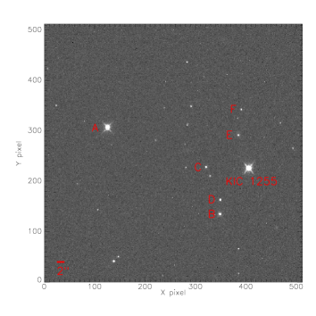
Figure 6.— The full frame array of our HST/WFC3 1.4 $\mu m$ photometry. The target star, as well as the handful of nearby reference stars (as listed in Table 2) that we perform photometry on to rule out false-positive scenarios, are labeled with letters from A-F.

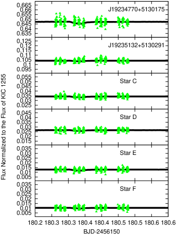
Figure 7.— HST F140W filter photometry of various reference stars (listed in Table 2) to KIC 1255. The solid black line denotes the 3$\sigma$ upper-limit on the transit depth obtained by scaling the mean of the short-cadence, phase-folded Kepler light curve (see $\S$2.1).

Table 2HST photometry of reference stars to KIC 1255

Star Name	Angular Separation	$A$	$t_{transit}$	$y_{o}$	3$\sigma$ upper-limit	Percentage Brightness
	From KIC 1255 (″)		(BJD-2456150)		on $A$	of KIC 1255 at $\sim$1.39 $\mu m$
Star A (2Mass J19234770+5130175)	39.15	0.116${}^{+0.097}_{-0.084}$	179.969	-0.35279${}^{+0.00022}_{-0.00016}$	0.375	64.7
Star B (2Mass J19235132+5130291)	13.40	0.012${}^{+0.021}_{-0.011}$	179.969	-0.89589${}^{+0.00010}_{-0.00010}$	0.112	10.4
Star C	11.34	0.052${}^{+0.053}_{-0.030}$	179.969	-0.96580${}^{+0.00010}_{-0.00010}$	0.183	3.4
Star D	10.69	0.030${}^{+0.039}_{-0.024}$	179.969	-0.97340${}^{+0.00011}_{-0.00011}$	0.158	2.7
Star E	8.39	0.065${}^{+0.056}_{-0.043}$	179.969	-0.98720${}^{+0.00010}_{-0.00012}$	0.209	1.3
Star F	14.28	0.009${}^{+0.018}_{-0.017}$	179.969	-0.98967${}^{+0.00010}_{-0.00010}$	0.117	1.0

We obtained HST/WFC3 photometry over four HST orbits of the transit of KIC 1255 in the F140W filter ($\lambda$$\sim$1.39 $\mu m$) on 2013 February 6 (UTC). The exposure times were 4.27 seconds; observations were obtained every 22.98 seconds, resulting in a duty cycle of $\sim$19%. 252 observations were obtained over the four HST orbits, or 63 observations per orbit. We performed aperture photometry, as described above in $\S$2.2. We use an aperture radius of 5.75 pixels; we do not subtract the background with an annulus, or otherwise. The results are nearly identical whether we do or do not subtract the background with an annulus with our aperture photometry. The HST photometry of KIC 1255 is presented in Figure 3, as well as the best-fit scaled version of the mean short-cadence, phase-folded Kepler photometry ($g(t)$; $\S$2.1); the associated parameters are listed in Table 1. We are unable to detect the transit of KIC 1255 in either our HST photometry or the simultaneous Kepler photometry (on 2013 February 6). We place a 3$\sigma$ upper limit on the transit depths on these two occasions of: $A$ $<$ 0.354 for our HST photometry, and $A$ $<$ 0.474 for our Kepler Transit #3. We note that the transit of KIC 1255b that we observed with HST and Kepler happened to be during a stretch of time where the KIC 1255b transit depth was below detectability for a number of transits in a row (approximately $\sim$5 days before and after our observed transit).

To rule out whether the transit that we associate with KIC 1255 is actually due to a nearby object, we also perform photometry on all relatively bright stars nearby to KIC 1255 in the HST photometry. By using the centroiding analysis methods of (Jenkins et al., 2010) on the Kepler photometry of KIC 1255, Rappaport et al. (2012) report that any background source that is causing the transits that we associate with KIC 1255 must be within 2″ of KIC 1255. As we discuss in $\S$2.3.2 we rule out sufficiently bright (at least 1% of the flux of KIC 1255) reference stars down to 0.2″ from KIC 1255, and a cursory inspection of Figure 6 indicates there are no sufficiently bright reference stars out to 11″ from KIC 1255. Objects fainter than 1% of KIC 1255, if fully occulted, would not be able to account for the greater than 1% transit depth observed in the Kepler photometry. Despite the fact that during our HST observations our HST and Kepler photometry did not display a detectable transit of KIC 1255b, we nevertheless perform photometry on all relatively bright stars that are within 20″of KIC 1255, and a few select stars of comparable brightness to KIC 1255 that are captured in our HST photometry. F140W photometry on all these stars from orbits 2-5 is presented in Figure 7. We display these stars in Figure 6, which shows the median full-frame image of all our HST F140W photometry. The 3$\sigma$ upper-limits on the transit depth for these stars are given in Table 2. None of these stars displays obvious behaviour that would suggest that they serve as a false positive for the characteristic photometry that we associate with KIC 1255b.

2.3.2 HST high-angular resolution imaging

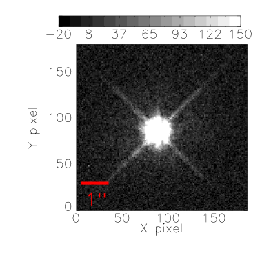
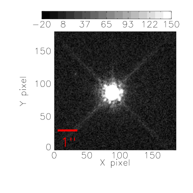
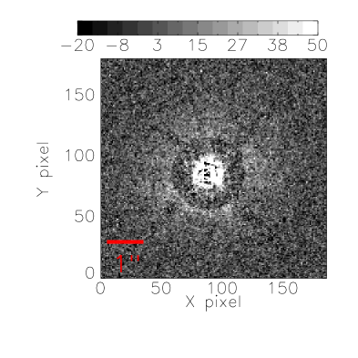
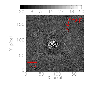
Figure 8.— HST/WFC3 high angular resolution imaging of KIC 1255 in the F555W channel (left), and the F775W channel (right). The top row of images are the AstroDrizzled images, while the bottom row of images are the PSF subtracted images. For both set of images, the scale is indicated at top, in units of electrons. The compass rose for all panels is given in the lower-right panel. For reference in the F775W difference image (bottom-right) the object at 10 o’clock at 2$\farcs$2 separation is at a delta-magnitude of 9.1, and is thus too faint, by a factor of more than $\sim$50, to cause the transit we associate with KIC 1255b.

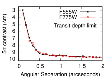
Figure 9.— Contrast limits for our HST/WFC3 high angular resolution imaging on nearby background/foreground companions to KIC 1255 in difference of magnitude in the F555W channel (red solid line, unfilled squares), and the F775W channel (black solid line, crosses). The horizontal dashed line denotes the limiting magnitude of the faintest object that could produce the transits we associated with KIC 1255b. We rule out companions bright enough to cause the transit we associate with KIC 1255b for separations greater than 0.2″(5$\sigma$).

HST high-angular resolution imaging observations to search for nearby companions to KIC 1255 were obtained with the WFC3 instrument in the following filters in the Infrared channel (IR): F125W ($\lambda$$\sim$1.25 $\mu m$), F140W ($\lambda$$\sim$1.39 $\mu m$), F160W ($\lambda$$\sim$1.54 $\mu m$), and the following filters in the ultraviolet and visible (UVIS) channel: F555W ($\lambda$$\sim$0.531 $\mu m$), F775W ($\lambda$$\sim$0.765 $\mu m$). We present results of the reduction and analysis of the F555W and F775W channels here.

Through program GO-12893, which imaged some of Kepler’s best Kepler Objects of Interest (KOIs) in terms of small planet candidates on long orbits, we had available F555W and F775W observations of many targets taken with exactly the same dither pattern and essentially the same signal-to-noise. We searched for a subset of the GO-12893 observations for which the target: (a) seemed to be an isolated single star, (b) had a $g-r$ color similar to KIC 1255, and (c) for which the HST focus offset matched that for KIC 1255. Visits number 60 (KIC 8150320), 94 (KIC 4139816), and 98 (KIC 5942949) met these criteria and were processed with AstroDrizzle (Fruchter et al., 2010) to the same 0$\farcs$0333 scale used for the KIC 1255 images. All observations consisted of four dithered exposures in which the target was kept just under detector saturation, and a fifth exposure at twice saturation to bring up the wings. In each case the drizzle combination was done to provide a final image well centered on a pixel. The KIC 1255 direct imaging results are shown in the upper panels of Figure 8 for 460 seconds in F555W and 330 seconds in F775W. The combined images had a FWHM of $\sim$0$\farcs$075, and are given in units of electrons. The observations in the three GO-12893 controls were averaged together to define a PSF for each filter, then scaled to the intensity of the KIC 1255 images and subtracted to provide the difference images shown in the lower panels of Figure 8, in units of electrons. The subtraction is performed to a radius of 1$\farcs$0 at F555W and 1$\farcs$2 at F775W; this subtraction is extended to $\sim$3″along the diagonal diffraction spikes. For reference, the object at 10 o’clock at 2$\farcs$2 separation in Figure 8 of the F775W difference image is at a delta-magnitude of 9.1.

The difference images were used to derive 5$\sigma$ detection limits as a function of offset distance by evaluating what fluctuations in 3$\times$3 0$\farcs$0333 pixels would stand out at this level relative to the scatter in successive 0$\farcs$08 annuli starting with one centered at 0$\farcs$1 (Gilliland & Rajan, 2011). These contrast limits are presented in Figure 9. The HST imaging ruled out potential sources of background false positives down to 0$\farcs$2 for a delta-magnitude of 4.7 (equivalent to the maximum observed Kepler transit depth), thereby reducing the original 2″ radius area in which these background/foreground candidates could exist by 99% (i.e., $<$0.2″).

2.4. Keck Adaptive Optics Imaging

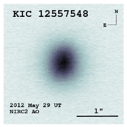
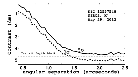
Figure 10.— Keck/NIRC2 high angular resolution imaging (left) of KIC 1255 in the K’ filter ($\lambda_{c}=$2.124 $\mu m$). The associated contrast limits on nearby background/foreground companions to KIC 1255 (right) in difference of magnitude in the K’ filter are given with 5$\sigma$ (solid line) and 3$\sigma$ confidence (thick-dashed line); the thin-dashed horizontal line denotes the limiting magnitude of the faintest object that could produce the transits we associated with KIC 1255b. We rule out companions that bright at this wavelength for separations greater than 1.4″(3$\sigma$).

We obtained high angular-resolution, near-infrared images of KIC 1255 on 2012 May 29 UT using NIRC2 (PI: Keith Matthews) and the Keck II adaptive optics (AO) system (Wizinowich et al. 2000). Observations were acquired in natural guide star mode with the K’ filter ($\lambda\sim$2.124 $\mu m$). Given the faintness of KIC 1255 (R=15.30), we opened the deformable mirror loops and applied tip/tilt correction commands only. Images were recorded using the narrow camera mode which provides a 10 mas plate scale. A standard 3-point dither pattern was executed to remove background radiation from the sky and instrument optics. A total on-source integration time of 360 seconds was obtained from 6 separate frames. Images were processed using standard techniques to replace hot pixel values, flat-field, subtract the background, and align and coadd frames (Crepp et al., 2012).

Figure 10 shows the final reduced image (left panel) along with sensitivity to off-axis sources (right panel). No obvious companions were noticed in either raw or processed frames. Comparing residual scattered light levels to the stellar peak intensity, our NIRC2 observations rule out the presence of possible photometric contaminants, at differential flux values comparable to and brighter than the maximum Kepler transit depth ($\Delta m=4.7$), for separations $>1.4$″ at $3\sigma$.

2.5. Keck Radial Velocities

Figure 11.— Constraints on the minimum mass, $m\,\sin$$i$, and period, $P$, of possible companions to KIC 1255. These are based on the Keck/HIRES RV measurements that we obtained with telluric-calibrated spectra. Artificial radial velocity signals were injected into the data and were recovered 50% of the time (dashed line), and 90% of the time (solid-line) with strong confidence (at a threshold greater than 3$\sigma$). We are able to rule-out giant planetary mass companions at periods $\lesssim 40$ days, and low-mass stellar companions ($m\,\sin i\sim 0.2\,M_{\odot}$) for $\lesssim 10$ year orbits with 90% confidence.

We obtained five high-resolution spectra of KIC 1255 using HIRES (Vogt et al., 1994) on the Keck I Telescope to measure absolute radial velocities. The exposures were 5–10 minutes in duration and achieved signal-to-noise ratios of 12–16 per pixel in $R$-band (on blaze). We followed the standard techniques of the California Planet Survey for the reduction and sky subtraction of spectra (Batalha et al., 2011). We measured absolute radial velocities (RVs) with the telluric oxygen A and B bands (759.4–762.1 nm and 686.7–688.4 nm) as a wavelength reference using the method of Chubak et al. (2012). The photon-weighted times of observation, RVs, and errors are listed in Table 3. Individual measurements carry 0.1 km s^-1 uncertainties, as demonstrated by bright standard star measurements (Chubak et al., 2012) as well as measurements of faint stars such as Kepler-78 ($V$ = 12; Howard et al. 2013).

The RV measurements of KIC 1255 span 512 days and have an RMS of 0.17 km s^-1. We searched for accelerations in the RV time series that could indicate a stellar-mass, long-period companion. A linear least-squares fit to the data yields a statistically insignificant slope of $-0.16\pm 0.90$ km s^-1 yr^-1. We then injected artificial RV signals for a hypothetical companion, with a given period, $P$, and minimum mass, $m\,\sin$$i$ (where $i$ is the orbital inclination of the companion), into the data and determined with what confidence we would be able to detect these companions. Zero-eccentricity orbits were assumed, and $4000$ trials were drawn with a random orbital phase. Inspired by a similar method used by Bean et al. (2010), signals were judged to be detected if the $\chi^{2}$ of the RV fit after subtracting the mean, $\chi_{RV}^{2}$, were greater than the $\chi^{2}$ of a straight line fit, $\chi_{straight}^{2}$, plus an amount corresponding to 3$\sigma$ confidence for four degrees of freedom (from our five data-points) – that is if: $\chi_{RV}^{2}$ $>$ $\chi_{straight}^{2}$ + 16.3. The resulting 50% and 90% confidence limits are given in Figure 11; stronger confidence limits (e.g. 99.73%) result in considerably higher-masses, as the time-gaps in the RV data allow for even very massive companions to slip through a small fraction of the time. Also, allowing eccentric orbits would result in less constraining (higher mass) limits at a given orbital period. Our analysis rules out giant planetary-mass companions ($m\,\sin$$i$ $\sim$ 13 M_J [Jupiter masses]) for $\lesssim 40$ day orbits, and low-mass stellar companions ($m\,\sin$$i$ $\sim$ 0.2 M_⊙ or greater) for $\lesssim 10$ year orbits with 90% confidence. We note an M-dwarf companion with a mass less than 0.2 M_⊙ would verge on the limit of being too faint to cause the 1% transit depth we associate with KIC 1255.

2.5.1 Radial Velocity Limit on KIC 1255b’s minimum mass

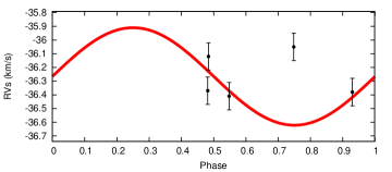
Figure 12.— The Keck/HIRES RV measurements phased to the orbital period of the candidate planet ($P$$\sim$0.6536 $d$). The red-solid line represents the radial velocity fit corresponding to the upper-limit on the mass of the candidate planet ($m\,\sin i$ $\lesssim$ 1.2 M_J) that we can rule-out with 3$\sigma$ certainty, for a circular orbit.

Our Keck RV measurements also allow us to attempt to detect, or set an upper limit on, the mass of the candidate planet KIC 1255b. Our Keck RVs phased to the orbital period of KIC 1255b are displayed in Figure 12. Similar to the techniques used above, we then insert circular (zero eccentricity) RV signals at KIC 1255b’s orbital period, and phase, until these signals exceed the chi-squared limit discussed in $\S$2.5. Our 3$\sigma$ upper limit on KIC 1255b’s minimum mass from the Keck RVs is then approximately 1.2 Jupiter-masses ($m\,\sin i$ $\lesssim$ 1.2 M_J), as displayed in Figure 12. We note that given the sparse RV sampling, allowing eccentric orbits would result in a much higher upper limit on KIC 1255b’s minimum mass. Given KIC 1255b’s close orbit with its parent star, one would not necessarily expect KIC 1255b to have an eccentric orbit; however the planet’s high mass loss rate, suggests a short life-time for the planet in its present orbit (Perez-Becker & Chiang, 2013), leaving open the possibility that the planet’s orbit may not have circularized yet.

Table 3Telluric-calibrated Radial Velocities from Keck-HIRES

JD – 2440000	Absolute Radial Velocity	Uncertainty
	(km s-1)	(km s-1)
16020.05982	$-$36.05	0.10
16028.02128	$-$36.38	0.10
16076.09278	$-$36.12	0.10
16110.07628	$-$36.37	0.10
16532.97013	$-$36.41	0.10

3. Multiwavelength Photometric Results

Table 4$A$ ratios for KIC 1255

Data & Transit #	Ratio
CFHT & Kepler Transit #1	$A_{Corr}$/$A_{Kepler}$ = 1.05 $\pm$ 0.36
CFHT & Kepler Transit #2	$A_{Corr}$/$A_{Kepler}$ = 0.97 $\pm$ 0.24
CFHT & Kepler Transits Combined	$A_{CFHT}$/$A_{Kepler}$ = 1.02 $\pm$ 0.20
HST & Kepler Transit	$A_{HST}$/$A_{Kepler}$ = 0.39 $\pm$ 0.46

Our simultaneous Kepler ($\sim$0.6 $\mu m$) and CFHT ($\sim$2.15 $\mu m$) photometry, and our simultaneous Kepler and HST ($\sim$1.4 $\mu m$) photometry allow us to compare the transit depths from the optical to the near-infrared. The ratio of the Kepler to the CFHT transit depth is similar in both our first & second CFHT and Kepler observations ($A_{Corr}$/$A_{Kepler}$ = 0.97 $\pm$ 0.36 on 2012 August 13 2012 and $A_{Corr}$/$A_{Kepler}$ = 1.05 $\pm$ 0.36 on 2012 September 1 2012). The weighted mean of the $A$ ratio from both observations is: $A_{CFHT}$/$A_{Kepler}$ = 1.02 $\pm$ 0.20. For the simultaneous HST and Kepler observation we are only able to return a null-detection of the transit depth at those wavelengths; the associated ratio of the HST to Kepler transit depths is: $A_{HST}$/$A_{Kepler}$ = 0.39 $\pm$ 0.46. Therefore, we can only say that there is no evidence for strongly different transit depths at these wavelengths. We summarize the ratios at these wavelengths in Table 4.

4. Limits on nearby companions to KIC 1255b and false positive scenarios

Although we know of no viable binary or higher-order multiple scenario that could explain the unusual photometry we observe for KIC 1255, we note that our high-angular resolution imaging, RVs, and multiwavelength photometry place strict limits on companions to KIC 1255 and thus on suggested false positive scenarios.

We searched for nearby companions to KIC 1255 with our HST/WFC3 and Keck/NIRC2 high-angular resolution imaging. With a maximum transit depth of 1.3% of the stellar flux, the maximum magnitude differential between a background object and KIC 1255 that could be causing the behaviour we observe is 4.7 magnitudes. Therefore our HST/WFC3 high angular resolution F555W, and F775W ($\lambda$$\sim$0.765 $\mu m$) imaging is able to rule out companions this bright with 5$\sigma$ confidence down to 0.2″ angular separation from KIC 1255b (see Figure 9).

In the near-infrared, given the CFHT to Kepler transit depth ratio we measure here ($A_{CFHT}$/$A_{Kepler}$ = 1.02 $\pm$ 0.20), we can expect that any object must be no more than 4.7 magnitudes fainter than KIC 1255b at these wavelengths as well; therefore for our Keck/NIRC2 imaging we are able to rule out companions this bright down to 1.4″ separation at 3$\sigma$ confidence.

Our radial-velocity observations allow us to rule-out low mass stellar companions ($\sim$ 0.2 M_⊙) for reasonably edge-on orbits, for periods less than $10$ years (this corresponds to $\lesssim$4 AU using the 0.7 $M_{\odot}$ stellar mass reported by Rappaport et al. 2012). Our high angular-resolution HST imaging limit of 0.2″, corresponds to $>$94 AU at the $\sim$470 parsec distance of KIC 1255 quoted by Rappaport et al. (2012). We therefore note there is little viable parameter space (only companion separations, $s$, of 4 AU$\lesssim$ $s$ $\lesssim$ 94 AU remain viable) for a binary or higher-order multiple companion to KIC 1255b that could be masquerading as a false-positive for the photometry of KIC 1255 that we associate with a disintegrating low-mass planet.

Lastly, we note that the fact that our near-infrared and optical photometry report similar transit depths, also allows us to place an additional constraint on hierarchical triple or background binary configurations with stars of different spectral types. For instance, if the photometry we associate with KIC 1255b was somehow due to a pair of late M-dwarfs (an effective temperature of $T_{\rm eff}$$\sim$3000 K) eclipsing one another, whose light was diluted by the K-dwarf star KIC 1255 ($T_{\rm eff}$ $\sim$ 4400 K; Rappaport et al. 2012), the $\sim$1% optical transit depths, would result in $\sim$6% transit depths at 2.15 $\mu m$ - a depth we can rule with very high confidence ($\sim$25$\sigma$). Similar limits could be set on a background binary that is of a different spectral type from KIC 1255. A background binary of similar spectral type to KIC 1255 remains a possible false positive; however it is unclear how such a scenario would explain the variable transit depths, and asymmetric transit profile we observe with this candidate planet.

With these stringent limits on false positive scenarios, we therefore conclude that the disintegrating low-mass planet scenario is the simplest explanation suggested to date for the Kepler photometry, and our multiwavelength photometry, RVs, and high angular-resolution imaging.

5. Discussion

5.1. Size of grains in the dust tail of KIC 1255b

The wavelength dependence of extinction by dust grains can provide information on their size and, in some cases, their composition (e.g., for interstellar grains see Mathis et al., 1977). This is due to the fact that the efficiency of scattering generally diminishes as the observational wavelength approaches the approximate particle circumference (Hansen & Travis, 1974), For this reason, the nearly identical transit depths we measure at $\lambda$ $\sim$0.6 $\mu m$ with Kepler and at $\lambda$ $\sim$2.15 $\mu m$ with CFHT/WIRCam allow us to set a lower-limit on the largest particles in the hypothetical dust tail trailing KIC 1255b. We set this lower-limit on the size assuming that all the dust particles are a single, identical size in $\S$5.1.3, and for a distribution of particle sizes in $\S$5.1.4.

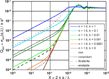
Figure 13.— The extinction efficiency, $Q_{ext}$ (Mie extinction cross sections, normalized to the geometric area of the grain), as a function of the nondimensional grain size parameter, $X=2\pi a/\lambda$, where $a$ is the radius of the grain, and $\lambda$ is the wavelength of observation. The dotted, short-dashed, long-dashed, and dot-dashed lines indicate the extinction efficiency of iron, corundum, forsterite and enstatite, as calculated as described in the text.

5.1.1 Spectral Dependence of Extinction

Table 5Wavelength Extinction and Sensitivity Limits

Parameter region	$\sigma_{ext}(a,\lambda)$	$\alpha(a,\lambda_{1},\lambda_{2})$
$a\gg\lambda/2\pi$	$2\pi a^{2}$	$0$
$a\ll\lambda/2\pi$ and $k=0$	$\propto$ $a^{6}/\lambda^{4}$	$4$
$a\ll\lambda/2\pi$ and $k\neq 0$	$\propto$ $a^{3}/\lambda$	$1$

The extinction (scattering plus absorption) of light by dust grains is a function of the wavelength, $\lambda$, of the light, the size of the grains, denoted by the grain radius, $a$, and the complex index of refraction of the dust material, where $n$ denotes the real component and $k$ the imaginary component. While there is also some dependence of extinction upon the shape of the dust grains, for simplicity we will only consider spherical grains here, and employ the Mie algorithm presented by Bohren & Huffman (1983) to calculate their cross sections. Fig. 13 plots the extinction efficiency (the ratio of the extinction cross section to the geometric cross section), $Q_{ext}(a,\lambda)=\sigma_{ext}(a,\lambda)/(\pi\,a^{2})$, as a function of the nondimensional size, $X=2\pi a/\lambda$, for grains with n = 1.6, and k = 0 (no absorption) and k varying from 0.0001 (low absorption) to 1 (highly absorbing).

We note that for large grains ($X\gg 1$; the right-hand side of the plot), the extinction cross-section is approximately constant ($Q_{ext}(a,\lambda)=\sigma_{ext}(a,\lambda)/(\pi\,a^{2})\rightarrow 2$) and only slightly dependent on wavelength, regardless of the absorption, $k$. For wavelengths longer or approaching the approximate particle circumference (the left side of the plot), the amount of extinction nominally depends on the amount of absorption (e.g., van de Hulst, 1981). Nonetheless, even for a great deal of absorption (i.e., $k$=1; the dark blue line in Figure 13), the extinction cross-section falls sharply for wavelengths longer than the approximate particle circumference; for low levels of absorption or none at all (the light green, orange, and red lines in Figure 13), the fall-off is even steeper. The asymptotic limits apparent in the plot are listed in Table 5. Therefore we surmise based on the nearly equal Kepler and CFHT transit depths, and thus the near equal levels of extinction between these two wavelengths, that our observations probe the right-hand side of the plot; we can therefore set a lower-limit on the largest particles in the hypothetical dust-tail trailing KIC 1255b.

For the scattering calculations that follow, we assume typical values for the complex index of refraction, $n$ and $k$, based on the values for typical Earth-abundant refractory materials, such as olivines and pyroxenes. Across our wavelength range of interest ($\lambda$=0.6 to 2.15 $\mu m$), for these materials, the imaginary component of the index of refraction is typically small, $k$ $\lesssim$ 0.02, while the real component of the index of refraction is often approximately n$\sim$1.6 (Kimura et al. 2002 and references therein). We also repeat our scattering calculations for a number of materials that have previously been suggested to be responsible for the dust supposedly trailing KIC 1255b. Four such materials, suggested by Budaj (2013), are forsterite (Mg₂SiO₄; a silicate from the olivine family), enstatite (MgSiO₃; a pyroxene without iron), pure iron, and corundum (Al₂O₃; a crystalline form of aluminium oxide). Three of these materials have similar complex indices of refraction across our wavelength range of interest ($\lambda$=0.6 to 2.15 $\mu m$): that is n$\sim$1.6 and $k$$<$10^-4 for enstatite (Dorschner et al., 1995), n$\sim$1.6 and $k$$<$10^-3 for forsterite (Jager et al., 2003), n$\sim$1.6 and $k$$<$0.04 for corundum (Koike et al., 2010). Pure iron is an outlier with n$\sim$2.9 - 3.9 and $k$$\sim$3.4 - 7.0 (Ordal, 1988) for wavelengths from $\lambda$=0.6 to 2.15 $\mu m$. In Figure 13 we also display the resulting extinction efficiency, $Q_{ext}(a,\lambda)$, of these materials.

5.1.2 Extinction Wavelength Dependence

To parameterize the amount of extinction between our two wavelengths, $\lambda_{1}$ and $\lambda_{2}$, we employ the Ångström exponent, $\alpha(a,\lambda_{1},\lambda_{2})$, a measure of the dependence of extinction on wavelength, defined as follows:

$$\alpha(a,\lambda_{1},\lambda_{2})\equiv-\frac{\log{[\sigma_{ext}(a,\lambda_{2})/\sigma_{ext}(a,\lambda_{1})]}}{\log{(\lambda_{2}/\lambda_{1})}}$$ (2)

The ratio of the transit depths in Table 4 is approximately the ratio of the extinctions at these two wavelengths, $\sigma_{ext}(a,\lambda_{2})/\sigma_{ext}(a,\lambda_{1})=1.02\pm 0.20$. Therefore, the associated value of $\alpha(a,0.6\,{\rm\mu m},2.15\,{\rm\mu m})=-0.02$ with ranges $-0.16$ to $0.16$ ($1\sigma$), $-0.27$ to $0.37$ ($2\sigma$), and $-0.38$ to $0.68$ ($3\sigma$).

5.1.3 Single Size Grains

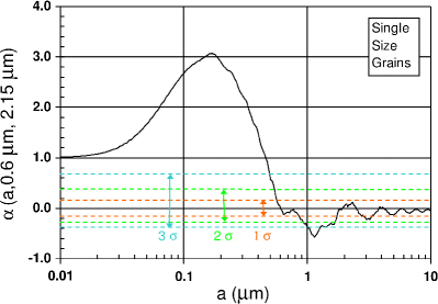
Figure 14.— Plot of the Ångström exponent for spherical grains of radius, $a$. We assume an index of refraction of $n=1.6$, and an imaginary component of the index of refraction of $k=0.02$. The horizontal orange, green, and blue dashed lines show the 1$\sigma$, 2$\sigma$, and 3$\sigma$ limits on $\alpha(a,\lambda_{1},\lambda_{2})$, respectively, from $\S$5.1.2. Grains of a single-size have to be larger than $a$$\gtrsim 0.5$ $\mu m$ (3$\sigma$) to be consistent with the ratio of our CFHT/WIRCam and Kepler transit depths.

What is the maximum size of particles in the hypothetical dust tail of KIC 1255b if the tail is composed solely of single-size spherical particles? Fig. 14 plots Mie calculations of $\alpha(a,0.6\,{\rm\mu m},2.15\,{\rm\mu m})$ for grains with $n=1.6$, $k=0.02$, and radius $a$. The 1, 2, and 3$\sigma$ error bars on $\alpha(a,0.6\,{\rm\mu m},2.15\,{\rm\mu m})$ are displayed with the dashed orange, green, and blue lines, respectively, in Figure 14. Therefore, for a dust tail consisting of single size grains their radius would have to be $\gtrsim 0.5$ ${\rm\mu m}$ (3$\sigma$).

We have also reproduced these scattering calculations for four materials that have been suggested to make-up the particles trailing KIC 1255b (these are corundum, pure iron, forsterite and enstatite), rather than for our hypothetical $n=1.6$ and $k$=0.02 material. Due to the close agreement between the complex index of refraction of forsterite, enstatite and corundum and our assumed $n=1.6$ and $k$=0.02 values, the size limit on single-sized forsterite, enstatite or corundum particles is indistinguishable from our hypothetical material; that is such grains must be $\gtrsim 0.5$ ${\rm\mu m}$ (3$\sigma$ confidence). Pure iron, on the other hand, which has a complex index of refraction that differs significantly from the above values, results in a less stringent limit on single size iron particles; pure iron particles would have to be $\gtrsim 0.2$ ${\rm\mu m}$ (3$\sigma$). However, due to iron’s high vapour pressure, we find it doubtful that pure iron particles could survive the high temperatures of a dust tail trailing KIC 1255b in the first place without sublimating. We therefore quote only our $\gtrsim 0.5$ ${\rm\mu m}$ (3$\sigma$) size-limit on single-size particles, henceforth.

5.1.4 Grain Size Distributions

We concede that a distribution consisting only of a single size of grain may not be the most realistic assumption for the hypothetical grains trailing KIC 1255b. Therefore, we also consider a range of particle sizes – specifically we consider grains with a specific particle size distribution denoted by a power-law with slopes, $\nu$, formally defined below. Power-law size distributions have been used in a diverse range of applications, for example: to model interstellar dust grains ($\nu$ $\sim$ 3.3 - 3.6; Mathis et al. 1977; Bierman & Harwit 1980), large particles in the comas of comets ($\nu$ $\sim$ 4.7 for particles 1 $\mu m$ to 1 $mm$ in size for the comet 103P/Hartley 2; Kelley et al. 2013), and dust (aerosols) in the Earth’s lower atmosphere from a world-wide network of ground-based Sun photometers ($3\leq\nu\leq 5$; Liou 2002; Holben et al. 1998).

We consider a distribution of grains ranging in size from $a=a_{min}$ to $a_{max}$. Let $N(a)$ be the number density of grains per unit grain radius and per unit area of the column along the path connecting the observer to the star. The average extinction cross section for the distribution, $\overline{\sigma}_{ext}(a_{min},a_{max},\lambda)$, is given by:

$$\overline{\sigma}_{ext}(a_{min},a_{max},\lambda)=\frac{\int_{a_{min}}^{a_{max}}N(a^{\prime})\,\sigma_{ext}(a^{\prime},\lambda)\,da^{\prime}}{\int_{a_{min}}^{a_{max}}N(a^{\prime})\,da^{\prime}}$$ (3)

where the overbar indicates the normalized average over the grain size distribution. The definition of Ångström exponent is readily adapted to distributions by replacing $\sigma_{ext}(a,\lambda)$ with $\overline{\sigma}_{ext}(a_{min},a_{max},\lambda)$ in Eqn. 2:

$$\alpha(a_{min},a_{max},\lambda_{1},\lambda_{2})\equiv$$

$$-\frac{\log{[\overline{\sigma}_{ext}(a_{min},a_{max},\lambda_{2})/\overline{\sigma}_{ext}(a_{min},a_{max},\lambda_{1})]}}{\log{(\lambda_{2}/\lambda_{1})}}$$ (4)

Likewise the first and second columns in Table 5 are readily adapted for size distributions by replacing $a$ by $\overline{a}$, $a^{2}$ by $\overline{a^{2}}$, and so on.

We now specialize to the case of a power-law distribution. We define the number density of particles of a given size as follows: $N(a)={\it c}\,a^{-\nu}$ for $a_{min}\leq a\leq a_{max}$, where the particle size distribution parameter, $\nu$, is taken to lie between $1\leq\nu\leq 5$, and ${\it c}$ is a normalization constant. In the following we arbitrarily set the minimum particle size to be $a_{min}=0.01\,{\rm\mu m}$, and set the maximum particle size to lie in an astrophysically plausible range of: $0.01\,{\rm\mu m}\leq a_{max}\leq 10\,{\rm\mu m}$. We calculate $\alpha(a_{min}=0.01\,{\rm\mu m},a_{max},\nu,0.6\,{\rm\mu m},2.15\,{\rm\mu m})$ for spherical grains comprised of material having $n=1.6$ and $k=0.02$, and plot the results in Figure 15. We note the similarity of this plot to the one for a single-sized particle in Fig. 14.

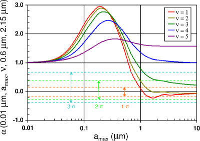
Figure 15.— Plot of extinction sensitivity for a range of particle size distributions with $\nu=1,\,2,\,3,\,4,\,{\rm and}\,5$. We employ an index of refraction of $n=1.6$, an imaginary component of the index of refraction, $k=0.02$, and calculate the particle distribution between a minimum radius of $a_{min}=0.01\,{\rm\mu m}$, and a maximum radius of $0.01\leq a_{max}\leq 10\,{\rm\mu m}$. The horizontal orange, green, and blue dashed lines show the 1$\sigma$, 2$\sigma$, and 3$\sigma$ limits on $\alpha(a_{min},a_{max},\nu,\lambda_{1},\lambda_{2})$, respectively, from $\S$5.1.4. Only smaller power-law slopes, and thus particle size distributions with more large particles, e.g. $\nu=1,\,2,$ & 3, result in a sufficient number of near-micron sized grains and thus satisfy the ratio of our CFHT/WIRCam and Kepler transit depths at the 3$\sigma$ level.

The implication is that there needs to be a sufficient proportion of grains with $a\gtrsim 1\,{\rm\mu m}$ for the ratio of the extinctions at the two wavelengths to be so close to $1$. In the case of a power-law grain size distribution this requires both a sufficiently large upper size cutoff, $a_{max}$, and a sufficiently small power-law slope, $\nu$. Note that in this limit the specific value of the imaginary component of the index of refraction, $k$, makes little difference.

At this point we note the important caveat that the wavelength sensitivity as defined in Eqn. 2 or 4 implicitly assumes that the dust tail is optically thin. The numerator in Eqn. 3 is the optical thickness, $\tau(\lambda)$, through the dust tail. Using the fact that the transmission $T(\lambda)\equiv\exp{[-\tau(\lambda)]}$ and that the extinction is $1-T(\lambda)$, we find that in the optically thin limit, i.e., where $\tau(\lambda)\ll 1$:

$$1-T(\lambda)\rightarrow\overline{\sigma}_{ext}(a_{min},a_{max},\lambda)\times\int_{a_{min}}^{a_{max}}N(a^{\prime})\,da^{\prime}\,\,\,\,$$

$${\rm if\,\,\tau(\lambda)\ll 1~{}~{}~{}}$$ (5)

Since the integral on the right in Eqn. 5 is independent of $\lambda$, extinction is proportional to $\overline{\sigma}_{ext}(a_{min},a_{max},\lambda)$ in this limit. However, since it is likely that the putative dust tail does not obscure the entire stellar surface there may be portions of the tail where the dust is optically thick, i.e., $\tau(\lambda)\gtrsim 1$. To the extent that this is the case, the extinction measurements will tend to give the same value independent of $\lambda$, the assumptions underlying $\alpha(\lambda_{1},\lambda_{2})$ break down, and the utility of $\alpha(\lambda_{1},\lambda_{2})$ for inferring grain size diminishes.

5.1.5 The impact of large particles on the supposed forward scattering peak

The presence of an increase in flux immediately preceding the dip attributable to strong forward scattering (Rappaport et al., 2012; Brogi et al., 2012; Budaj, 2013) is also suggestive of large particles since the strength of forward scattering is a strong function of grain size (e.g., DeVore, et al., 2013). We note that according to the model of Budaj (2013) there may be some tension between our finding of $a$$\gtrsim 0.5$ ${\rm\mu m}$ particles and the Kepler observations, as 0.1 - 1.0 $\mu m$ particles arguably over-predict the amount of forward scattering compared to the Kepler observations. However, the forward scattering increase also suggests that the dust responsible is not optically thick since scattering acts both to inhibit the forward scattered photons as well as cause the flux to diverge angularly. If multispectral measurements of the forward scattering peak were obtained with adequate signal to noise, then they could be used to provide information on grain size through the strong dependence of the angular spread of forward scattering on the ratio of the effective grain diameter to the wavelength.

5.2. KIC 1255b Particle Lifting

If the largest particles in the tail of KIC 1255b are at least 0.5 microns in size, then this raises the question of how such large particles were lofted from the planet in the first place. According to the hydrodynamic wind model of Perez-Becker & Chiang (2013), the present-day mass of KIC 1255b is $\lesssim 0.02M_{\oplus}$, or less than half the mass of Mercury. Only for masses this small are surface gravities weak enough to allow evaporative winds to blow with mass-loss rates satisfying the observations. These authors have already shown that spherical grains having radii of $1$ $\mu$m and bulk densities of $3$ g/cm³ could be dragged by winds outside the Roche lobe of KIC 1255b — albeit only marginally if the planet mass is near its upper limit. As the planet radius shrinks, the sizes of particles that can escape grow in inverse proportion (see their equation 30 and surrounding discussion). In sum, as long as the planet is small enough, micron-sized or larger particles can escape. Therefore, our observations suggest that the candidate planet KIC 1255b might best be described as a sub-Mercury — rather than super-Mercury — mass planet.

Note that the particles do not need to be lifted directly from the planetary surface, since the grains only condense at altitude, where the wind has an opportunity to cool adiabatically. Indeed the grains cannot be present at their maximum abundance (relative to gas) at the base of the wind; if they were, the flow would be so optically thick that the planetary surface would be shielded from starlight and would not heat to the temperatures required for an evaporative wind to be launched. In the wind solutions of Perez-Becker & Chiang (2013), the dust abundance increases by orders of magnitude from the surface to the Roche lobe (see their Figure 3). Thus the problem of lifting grains beyond the Roche lobe should only be a problem near the Roche lobe, and it is there that Perez-Becker & Chiang (2013) compare the drag force exerted by the wind with the planet’s tidally modified gravity. We suppose it is possible that the problem of lift can be avoided altogether if grains condense outside the Roche lobe. We cannot rule this possibility out since the grain condensation profile was merely parameterized by Perez-Becker & Chiang (2013), not solved from first principles.

5.3. Prospects for follow-up observations

The enlightening multi-wavelength observations presented in this paper were greatly facilitated by the impressive photometric capabilities of the Kepler spacecraft that allowed us to achieve simultaneous, accurate optical photometry in addition to our ground and spacebased photometry and imaging. With the recent malfunction of this spacecraft, prospects for illuminating follow-up studies of this object are much dimmer than previously, and may require much more difficult to schedule follow-up from several telescopes simultaneously.

Although the KIC 1255b transit does not appear to be strongly wavelength dependent from 0.6 - 2.15 $\mu m$, follow-up observations further into the infrared would be expected to show transit depth differences compared to those obtained simultaneously in the optical, unless the size of particles in the cometary tail are several microns in size. Such observations could be obtained with the Spitzer/IRAC (Fazio et al., 2004) instrument. We note that several micron-sized particles would be inconsistent with the size of the forward scattering peak observed with Kepler (Rappaport et al., 2012; Budaj, 2013) (unless there is evolution of the grain sizes along the tail). Low resolution spectroscopy over a wide spectral range, either from the ground or from space, would be useful to look for both wavelength dependent transit depth changes, and morphological changes in the photometry of the dust tail as revealed by the forward-scattering peak, and asymmetric egress of the transit. We note, that the strength of the forward scattering peak is also expected to be wavelength dependent, and observations with sufficient precision to look for such minute changes, would be highly illuminating.

6. Conclusions

We have presented multiwavelength photometry, high angular-resolution imaging and radial velocities of the intriguing disintegrating low-mass candidate planet KIC 1255b. We summarize our findings here:

(i) Comparison of our CFHT/WIRCam 2.15 $\mu m$ to Kepler 0.6 $\mu m$ transit depths, and the resulting constraints on particle sizes in the tail trailing KIC 1255b: The average ratio of the transit depths that we observe from the ground with CFHT/WIRCam and space with Kepler at our two epochs are: 1.02 $\pm$ 0.20. In the disintegrating planet scenario, the only way to see a lack of extinction from the optical to the near-infrared is if the circumference of the particles are at least approximately the wavelength of the observations. Therefore, if the transits we observe are due to scattering from single-size particles streaming from the planet in a comet-like tail, then the particles must be $\sim$0.5 microns in radius or larger. Similarly, if the particle size distribution in the tail follows a number density defined by a power-law, then only smaller power-law slopes, and thus larger particle sizes result in a sufficient number of near-micron sized grains to satisfy our observations.

(ii) Comparison of our HST 1.4 $\mu m$ and Kepler 0.6 $\mu m$ null detections: Unfortunately we were unable to detect the transit of KIC 1255b in either our simultaneous HST and Kepler photometry, due to the fact that the transits of KIC 1255b had largely disappeared in the Kepler photometry for approximately $\sim$5 days before and after our observed transit. We are therefore able to conclude little from these observations, other than there is no evidence for strongly different transit depths at these wavelengths.

(iii) Particle lifting from KIC 1255b: Perez-Becker & Chiang (2013) have already demonstrated that lifting particles nearly a micron in size is possible from KIC 1255b. As lifting such large particles becomes much more difficult as one increases the mass of the candidate planet, we note our $\gtrsim$0.5 micron limit on single-sized particles in the tail trailing KIC 1255b favours a sub-Mercury, rather than super-Mercury, mass for KIC 1255b.

(iv) Constraints on false-positives from our high angular-resolution imaging, RVs and photometry: Our HST ($\sim$0.53 $\mu m$ and $\sim$0.77 $\mu m$) high angular-resolution imaging allows us to rule-out background and foreground candidates at angular separations greater than 0.2″ that could be responsible for the transit we associate with a planet transiting KIC 1255b. The associated limit from our groundbased Keck/NIRC2 Adaptive Optics observations in K’-band ($\sim$2.12 $\mu m$) is for separations greater than 1.4″. Our radial velocity observations allow us to rule out low-mass stellar companions ($\gtrsim$ 0.2 M_⊙) for periods less than $\lesssim$$10$ years, and 13 Jupiter-mass companions for periods less than $\lesssim$$40$ days. Furthermore, the similar transit depths we observe in the near-infrared with CFHT/WIRCam and in the optical with Kepler also allow us to rule out background/foreground candidates, or higher-order multiples with significantly different spectral types, as this would result in a colour-dependent transit depth from the optical to the near-infrared. Although prior to these observations we knew of no viable false-positive scenario that could reproduce the unique photometry we observed with Kepler (e.g. the forward scattering bump before transit, the sharp ingress and gradual egress transit profile, the sharply varying transit depths), we note that we have now greatly reduced the parameter space for viable false positive scenarios. We conclude that the disintegrating low-mass planet scenario is the simplest explanation for our multiwavelength photometry, RVs and high angular-resolution imaging suggested to date.

(v) Limit on the mass of the candidate planet KIC 1255b: Our KECK/HIRES RVs of KIC 1255b allow us to place an upper-limit on the minimum mass of the candidate planet that confirms it is firmly in the planetary regime; this limit is $m\,\sin i$ $\lesssim$ 1.2 M_J with 3$\sigma$ confidence, assuming a circular orbit.

References

- Ångström (1929) Ångström, A. 1929, Geogr. Ann. 11, 156
- Batalha et al. (2011) Batalha, N. M., Borucki, W. J et al. 2011, ApJ, 729, 27
- Bean et al. (2010) Bean, J.L., Seifahrt, A. et al. 2010, ApJ, 711, L19
- Bierman & Harwit (1980) Bierman, P. & Harwit, M. 1980, ApJ, 241, L105
- Bohren & Huffman (1983) Bohren, C. F. & Huffman, D. R. 1983, Absorption and Scattering of Light by Small Particles, John Wiley & Sons, Inc., New York.
- Borucki et al. (2009) Borucki, W.J. et al. 2009, Science, 325, 709
- Brogi et al. (2012) Brogi, M. et al. 2012, A&A, 545, L5
- Budaj et al. (2012) Budaj, J. et al. 2012, A&A, 537, A115
- Budaj (2013) Budaj, J. 2013, A&A, 557, A72
- Chubak et al. (2012) Chubak, C., Marcy, G., Fischer, D. A., Howard, A. W. et al. 2012, arXiv:astro-ph/1207.6212
- Crepp et al. (2012) Crepp, J.R., Johnson, J.A., Howard, A.W. et al. 2012, ApJ, 761, 39
- Croll (2006) Croll, B. 2006, PASP, 118, 1351
- Croll et al. (2010a) Croll, B. et al. 2010a, ApJ, 717, 1084
- Croll et al. (2010b) Croll, B. et al. 2010b, ApJ, 718, 920
- DeVore (2011) DeVore, J.G. 2011, J. Atmos. Ocean. Tech., 28, 779
- DeVore, et al. (2013) DeVore, J.G., J.A. Kristl, & Rappaport, S.A. 2013, J. Geophys. Res, 118, 5679
- Dorschner et al. (1995) Dorschner, J., Begemann, B., Henning, T., Jaeger, C., Mutschke, H. 1995, A&A, 300, 503
- Dressel et al. (2010) Dressel, L., Wong, M., Pavlovsky, C., Long, K., et al. 2010, “Wide Field Camera 3 Instrument Handbook”, Version 2.1, (Baltimore: STScI)
- Fazio et al. (2004) Fazio, G. G., et al. 2004, ApJS, 154, 10
- Fruchter et al. (2010) Fruchter, A.S., Hack, W., Dencheva, N., Droettboom, M., Greenfield, P. 2010, in STScI Calibration Workshop Proceedings, eds. S. Deustua, & C. Oliveira, (Baltimore, MD: STScI), p. 376
- Gilliland & Rajan (2011) Gilliland, R.L., & Rajan, A. 2011, Instrument Science Report WFC3 2011-03 (Baltimore, MD: STScI)
- Holben et al. (1998) Holben, B. et al. 1998, Rem. Sens. Environ., 66, 1
- Hansen & Travis (1974) Hansen, J.E. & Travis, L.D. 1974, Space Science Reviews, 16, 527
- Howard et al. (2013) Howard, A.W., Sanchis-Ojeda, R., Marcy, G.W. et al. 2013, Nature, 503, 381
- Jager et al. (2003) Jager, C., Dorschner, J., Mutschke, H. et al. 2003, A&A, 408, 193
- Jenkins et al. (2010) Jenkins, J.M., Borucki, W. J., Koch, D. G., et al. 2010, ApJ, 724, 1108
- Junge (1963) Junge, C.E. 1963, Air Chemistry and Radioactivity, Academic Press, New York
- Kawahara et al. (2013) Kawahara, H. et al. 2013, arXiv:astro-ph/1308.1585
- Kelley et al. (2013) Kelley, M.S., Lindler, D.J., Bodewits, D. et al. 2013, Icarus, 222, 634
- Kimura et al. (2002) Kimura, H., Mann, I., Biesecker, D.A. & Jessberger, E.K. 2002, Icarus, 159, 529
- Kipping (2010) Kipping, D.M. 2010, MNRAS, 408, 1758
- Koike et al. (2010) Koike, C. 1995, Icarus, 114, 203
- Liou (2002) Liou. K.N. 2002, An Introduction to Atmospheric Radiation, Second Edition, Academic Press, San Diego, CA
- Mathis et al. (1977) Mathis, J. S., W. Rumpl, & Nordsieck, K. H. 1977, ApJ, 217, 425
- Montalto (2010) Montalto, M. 2010, A&A, 521, A60
- Ordal (1988) Ordal, M.A. 1988, Applied Optics, 27, 1203
- Perez-Becker & Chiang (2013) Perez-Becker, D. & Chiang, E. 2013, MNRAS, 433, 2294
- Perez-Becker & Showman (2013) Perez-Becker, D. & Showman, A.P. 2013, ApJ, 776, 134
- Puget et al. (2004) Puget, P. et al. 2004, SPIE, 5492, 978
- Rappaport et al. (2012) Rappaport, S. et al. 2012, ApJ, 752, 1
- Rappaport et al. (2014) Rappaport, S. et al. 2014, ApJ, 2014, arXiv:astro-ph/1312.2054
- Lord Rayleigh (1871) Rayleigh, Lord (1871), Philos. Mag., 41, 274.
- van de Hulst (1981) van de Hulst, H. C. 1981, Light Scattering by Small Particles, Dover Publications, Inc., New York.
- Vogt et al. (1994) Vogt, S.S., Allen, S.L., Bigelow, B.C. et al. 1994, in Proc. SPIE Instrumentation in Astronomy VIII, David L. Crawford; Eric R. Craine; Eds., Vol. 2198, p. 362
- van Werkhoven et al. (2013) van Werkhoven, T.I.M. et al. 2013, A&A, accepted, arXiv:astro-ph/1311.5688
- Winn et al. (2008) Winn, J.N. et al. 2008, ApJ, 683, 1076
- Wizinowich et al. (2000) Wizinowich, P., Acton, D. S., Shelton, C., et al. 2000, PASP, 112, 315