Consistent Testing for Recurrent Genomic Aberrations

Abstract

Genomic aberrations, such as somatic copy number alterations, are frequently observed in tumor tissue. Recurrent aberrations, occurring in the same region across multiple subjects, are of interest because they may highlight genes associated with tumor development or progression. A number of tools have been proposed to assess the statistical significance of recurrent DNA copy number aberrations, but their statistical properties have not been carefully studied. Cyclic shift testing, a permutation procedure using independent random shifts of genomic marker observations on the genome, has been proposed to identify recurrent aberrations, and is potentially useful for a wider variety of purposes, including identifying regions with methylation aberrations or overrepresented in disease association studies. For data following a countable-state Markov model, we prove the asymptotic validity of cyclic shift $p$-values under a fixed sample size regime as the number of observed markers tends to infinity. We illustrate cyclic shift testing for a variety of data types, producing biologically relevant findings for three publicly available datasets.

1 Introduction

Many genomic datasets consist of measurements from multiple samples at a common set of genetic markers, with no “phenotype” representing clinical state or experimental condition of the sample. Datasets of this type include genome-wide measurements of DNA copy number or DNA methylation, for which the main goal is to identify aberrant regions on the genome that tend to have extreme measurements in comparison to other regions. Testing for aberrations requires some thought about appropriate test statistics, and constructing a null distribution that appropriately reflects serial correlation structures inherent to genomic data. A meta-analysis across several genome-wide association studies might also be viewed in this framework, in the sense that the testing for association within each study produces a vector of $p$-values that might be viewed as a vector of “observations.”

The problem of interest to us is the identification of aberrant markers, where multiple samples exhibit a coordinated (unidirectional), departure from the expected state. Aberrant markers are of particular interest in cancer studies, where tumor suppressors or oncogenes exhibit DNA copy variation or modified methylation levels. Similarly, it may be possible to identify pleiotropic single nucleotide polymorphisms (SNPs) in disease association by identifying genetic markers that repeatedly give rise to small $p$-values in multiple association studies.

In this paper we provide a rigorous asymptotic analysis of a permutation based testing procedure for identifying aberrant markers in genomic data sets. The procedure, called DiNAMIC, was introduced in Walter et al. (2011), and is described in detail below. In contrast to other procedures which permute all observations, DiNAMIC is based on cyclic shifting of samples. Cyclic shifting eliminates concurrent findings across samples, but retains the adjacency of observations in a sample (with the exception of the first and last entries), thereby largely preserving the correlation structure among markers. Our principal result is that, for a broad family of null data distributions, the sampling distribution of the DiNAMIC procedure is close to the true conditional distribution of the data restricted to its cyclic shifts. As a corollary, we find that the cyclic shift testing provides asymptotically correct Type I error rates.

The outline of the paper is as follows. The next section is devoted to a description of the cyclic shift procedure, a discussion of the underlying testing framework within which our analysis is carried out, and a statement of our principal result. In Section 3 we apply cyclic shift testing to DNA copy number analysis, DNA methylation analysis, and meta-analysis of GWAS data, and show that the results are consistent with the existing biological literature. Because of its broad applicability and solid statistical foundation, we believe that cyclic shift testing is a valuable tool for the identification of aberrant markers in many large scale genomic studies.

2 Asymptotic Consistency of Cyclic Shift Permutation

2.1 Data Matrix

We consider a data set derived from $n$ subjects at $m$ common genomic locations or markers. The data is arranged in an $n\times m$ matrix $\bf X$ with values in a set $\cal{A}\subseteq\mathbb{R}$. Depending on the application, $\cal{A}$ may be finite or infinite. The entry $x_{ij}$ of $\bf X$ contains data from subject $i$ at marker $j$. Thus the $i$th row $\mbox{$\bf X$}_{i\cdot}$ of $\bf X$ contains the data from subject $i$ at all markers, and the $j$th column $\mbox{$\bf X$}_{\cdot j}$ of $\bf X$ contains the data at marker $j$ across subjects. For $1\leq j\leq m$ let $s_{j}=s_{j}(\mbox{$\bf X$}_{\cdot j})$ be a local summary statistic for the $j$th marker. In most applications the simple sum statistic $s_{j}=\sum_{i=1}^{n}x_{ij}$ is employed. In order to identify locations with coordinated departures from baseline behavior, we apply a global summary statistic to the local statistics $s_{1},\ldots,s_{m}$. When looking for extreme, positive departures from baseline it is natural to employ the global statistic

$$\mbox{$T({\bf X})$}\ =\ {\mathrm{max}}(s_{1},\dots,s_{m}).$$ (2.1)

To detect negative departures from baseline, the maximum may be replaced by a minimum. The cyclic shift procedure and the supporting theory in Theorem 1 apply to arbitrary local statistics, as well as a range of global statistics.

2.2 Cyclic Shift Testing

Given a data matrix $\bf X$, we are interested in assessing the significance of the observed value $t_{0}=T(\mbox{$\bf X$})$ of the global statistic. When $t_{0}$ is found to be significant, the identity and location of the marker $j$ having the maximum (or minimum) local statistic is of primary biological importance. While in special cases it is possible to compute $p$-values for $t_{0}$ under parametric assumptions, permutation based approaches are often an attractive and more flexible alternative. A permutation based $p$-value can be obtained by applying permutations $\pi$ to the entries of $\bf X$, producing the matrices $\pi(\mbox{$\bf X$})$, and then comparing $t_{0}$ to the resulting values $T(\pi(\mbox{$\bf X$}))$ of the global statistic. The maximum global statistic accounts for multiple comparisons across markers, so it is not necessary to apply further multiplicity correction to the permuted values $T(\pi(\mbox{$\bf X$}))$.

The performance and suitability of permutation based $p$-values in the marker identification problem depends critically on the family of allowable permutations $\pi$. If $\pi$ permutes the entries of $\bf X$ without preserving row or column membership, then the induced null distribution is equivalent to sampling the entries of $\bf X$ at random without replacement. In this case the induced null distribution does not capture the correlation of measurements within a sample, or systematic differences (e.g. in scale, location, correlation) between samples. In real data, correlations within and systematic differences between samples can be present even in the absence of aberrant markers. As such, $p$-values obtained under full permutation of $\bf X$ will be sensitive to secondary features of the data and may yields significant $p$-values even when no aberrant markers are present. An obvious improvement of full permutation is to separately permute the values in each row (sample) of the data matrix. This approach is used in the GISTIC procedure of Beroukhim et al. (2007). While row-by-row permutation preserves some differences between rows, it eliminates correlations within rows (and correlation differences between rows), so that the induced null distribution is again sensitive to secondary, correlation based features of the data that are not related to the presence of aberrant markers.

The DiNAMIC cyclic shift testing procedure of Walter et al. (2011) addresses the shortcomings of full and row-by-row permutation by further restricting the set of allowable permutations. In the procedure, each row of the data matrix is shifted to the left in a cyclic fashion, as detailed below, so that the first $k$ entries of the vector are placed after the last element; the values of the offsets $k$ are chosen independently from row to row. Cyclic shifting preserves the serial correlation structure with each sample, except at the single break point where the last and first elements of the unshifted sample are placed next to one another. At the same time, the use of different offsets breaks concurrency among the samples, so that the resulting cyclic null distribution is appropriate for testing the significance of $t_{0}=T(\mbox{$\bf X$})$.

2.3 Cyclic Shift Testing

Formally, a cyclic shift of index $k\in\{0,\ldots,m-1\}$ is a map $\sigma_{k}:{\cal{A}}^{m}\rightarrow{\cal{A}}^{m}$ whose action is defined as follows:

$$\sigma_{k}(x_{1},x_{2},\dots,x_{m})=(x_{k+1},x_{k+2},\dots,x_{m},x_{1},\dots,x_{k}).$$

Given $\mbox{$\bf k$}=(k_{1},\ldots,k_{n})$ with $k_{i}\in\{0,\ldots,m-1\}$, let $\sigma_{\mbox{\scriptsize\bf k}}=\sigma_{k_{1}}\otimes\cdots\otimes\sigma_{k_{n}}$ be the map from the set ${\cal{A}}^{n\times m}$ of data matrices to itself defined by applying $\sigma_{k_{i}}$ to the $i$th row of $\bf X$, namely,

$$\sigma_{\mbox{\scriptsize\bf k}}(\mbox{$\bf X$})\ =\ (\sigma_{k_{1}}(\mbox{$\bf X$}_{1\cdot}),\ldots,\sigma_{k_{n}}(\mbox{$\bf X$}_{n\cdot}))^{t}$$

The cyclic shift testing procedure of Walter et al. (2011) is as follows.

Cyclic shift procedure to assess the statistical significance of $T({\bf X})$

1. Let $\sigma^{1}(\cdot),\dots,\sigma^{N}(\cdot)$ be random cyclic shifts of the form $\sigma_{k_{1}}\otimes\cdots\otimes\sigma_{k_{n}}$, where $k_{1},\ldots,k_{n}$ are independent and each is chosen uniformly from $\{0,\ldots,m-1\}$.

2. Compute the values $T(\sigma^{1}(\mbox{$\bf X$})),\ldots,T(\sigma^{N}(\mbox{$\bf X$}))$ of the global statistic $T$ at the random cyclic shifts of $\bf X$.

3. Define the percentile-based $p$-value

   $$p(T(\mbox{$\bf X$}))=\max\left(N^{-1}\sum_{l=1}^{N}I(T(\sigma^{l}(\mbox{$\bf X$}))\geq T(\mbox{$\bf X$})),1/N\right).$$

   Here $I(A)$ is the indicator function of the event $A$.

2.4 Testing Framework

We wish to assess the performance of the cyclic shift procedure within a formal testing framework. To this end, we regard the observed data matrix $\bf X$ as an observation from a probability distribution $P_{m}$ on ${\cal A}^{n\times m}$, so that for any (measurable) set $A\subseteq{\cal A}^{n\times m}$ the probability $P_{m}(A)=\mathbb{P}(\mbox{$\bf X$}\in A).$ As measurements derived from distinct samples are typically independent, we restrict our attention to the family of measures ${\cal P}$ on ${\cal A}^{n\times m}$ under which the rows of $\bf X$ are independent.

Let ${\cal P}_{0}\subseteq{\cal P}$ be the sub-family of ${\cal P}$ corresponding to the null hypothesis that $\bf X$ has no atypical markers, i.e., no markers exhibiting coordinated activity across samples. One may define ${\cal P}_{0}$ in a variety of ways, but the simplest is to let ${\cal P}_{0}$ be the set of distributions $P_{m}\in{\cal P}$ such that the rows of $\bf X$ are stationary and ergodic under $P_{m}$; independence of the rows follows from the definition of ${\cal P}$. Under ${\cal P}_{0}$ the columns of $\bf X$ are stationary and ergodic, and the same is true of the local statistics $s_{j}$, which are identically distributed and have constant mean and variance. Thus under ${\cal P}_{0}$ no marker is atypical in a strong distributional sense.

Our principal result shows that the $p$-value produced by the cyclic shift procedure is approximately consistent for distributions $P_{m}$ in a subfamily ${\cal P}^{*}\subseteq{\cal P}_{0}$. The family ${\cal P}^{*}$ includes or approximates many distributions of practical interest, including finite order Markov chains with discrete or continuous state spaces. In order to assess the consistency of the cyclic shift $p$-value we carefully define both the target and the induced distributions of the procedure. As much of what follows concerns probabilities conditional on the observed data matrix, we use $\bf X$ to denote both the random matrix and its observed realization. Given $\bf X$ let

$${\cal S}_{m}(\mbox{$\bf X$})\ =\ \{\sigma_{\mbox{\scriptsize\bf k}}(\mbox{$\bf X$}):\mbox{$\bf k$}\in\{0,\ldots,m-1\}^{n}\}\ \subseteq\ {\cal A}^{n\times m}$$

be the set of all cyclic shifts of $\bf X$. Define the true conditional distribution to be the conditional distribution of $P_{m}$ given ${\cal S}_{m}(\mbox{$\bf X$})$, namely

$$P_{\mbox{\scriptsize\bf X}}(A)\ =\ P_{m}(A\,|\,{\cal S}_{m}(\mbox{$\bf X$}))\ \ \ \ A\subseteq{\cal A}^{n\times m}.$$

If $P_{m}$ is discrete with probability mass function $p(\cdot)$ then

$$P_{\mbox{\scriptsize\bf X}}(A)\ =\ \frac{1}{\sum_{{\bf Y}^{\prime}\in{\cal S}_{m}({\bf X})}p(\mbox{$\bf Y$}^{\prime})}\sum_{\mbox{\scriptsize\bf Y}\in A}p(\mbox{$\bf Y$})\cdot I(\mbox{$\bf Y$}\in{\cal S}_{m}(\mbox{$\bf X$})).$$

If $P_{m}$ has probability density function $f(\cdot)$ then $P_{\mbox{\scriptsize\bf X}}$ may be defined in a similar fashion.

In the cyclic shift procedure, matrices are selected uniformly at random from the set ${\cal S}_{m}(\mbox{$\bf X$})$ of cyclic shifts of the observed data matrix $\bf X$. The associated cyclic conditional distribution has the form

$$Q_{\mbox{\scriptsize\bf X}}(A)\ =\ \sum_{\mbox{\scriptsize\bf Y}\in A}\frac{1}{|{\cal S}_{m}(\mbox{$\bf X$})|}\cdot I(\mbox{$\bf Y$}\in A)\ \ \ A\subseteq{\cal A}^{n\times m}.$$

Under mild conditions the $m^{n}$ cyclic shifts of $\bf X$ are distinct with high probability when $m$ is large (see Lemma 3 in Section 4). In this case, the cyclic conditional distribution may be written as

$$Q_{\mbox{\scriptsize\bf X}}(A)\ =\ \sum_{\mbox{\scriptsize\bf Y}\in A}\frac{1}{m^{n}}\cdot I(\mbox{$\bf Y$}\in{\cal S}_{m}(\mbox{$\bf X$}))\ =\ \frac{1}{m^{n}}\cdot|A\cap{\cal S}_{m}(\mbox{$\bf X$})|\ \ \ \ A\subseteq{\cal A}^{n\times m}.$$

The distribution of the cyclic shift $p$-value is given by

$$p(T(\mbox{$\bf X$}))\sim\max(N^{-1}\,\mbox{Bin}(N,\alpha),1/N).$$

Here $\alpha=Q_{\mbox{\scriptsize\bf X}}(T\geq t_{0})$ where $t_{0}$ is the observed value of $T(\mbox{$\bf X$})$, and $T\geq t_{0}$ represents the event $\{\mbox{$\bf Y$}:T(\mbox{$\bf Y$})\geq t_{0}\}$. Note that as the number $N$ of cyclic shifts increases, the $p$-value $p(T(\mbox{$\bf X$}))$ will converge in probability to $Q_{\mbox{\scriptsize\bf X}}(T\geq t_{0})$

2.5 Principal Result

Our principal result requires an invariance condition on the global statistic $T$. Informally, the condition ensures that $T$ does not give special treatment to any column of the data matrix.

Definition: A statistic $T:{\cal A}^{n\times m}\to\mathbb{R}$ is invariant under constant shifts if $T(\mbox{$\bf X$})=T(\mbox{$\bf X$}^{\prime})$ whenever $\mbox{$\bf X$}^{\prime}$ is obtained from $\bf X$ by applying the same cyclic shift $\sigma_{k}(\cdot)$ to each row of $\bf X$.

The maximum column sum statistic used in the cyclic shift testing procedure is clearly invariant under constant shifts. More generally, any statistic of the form $T(\mbox{$\bf X$})=g(h(\mbox{$\bf X$}_{\cdot 1}),\ldots,h(\mbox{$\bf X$}_{\cdot m}))$ where $h:{\cal A}^{n}\to{\cal B}$ is an arbitrary local statistic (not necessarily a sum), and $g:{\cal B}^{m}\to\mathbb{R}$ is invariant under cyclic shifts will be invariant under constant shifts. The following result establishes the asymptotic validity of the cyclic shift procedure in this general setting.

Theorem 1.

Let $\bf X$ be a random $n\times m$ matrix whose rows $\mbox{$\bf X$}_{i\cdot}$ are independent copies of a first-order stationary ergodic Markov chain with countable state space ${\cal{A}}$ and transition probabilities $p(u|v)$. Suppose that

$$\max_{u,v\in{\cal{A}}}\ p(u|v)<1\ \mbox{ and }\ \frac{p_{1}(u)\,p_{1}(v)}{p_{2}(u,v)}<\infty\mbox{ for each $u,v\in{\cal{A}}$}$$ (2.2)

where in the second condition we define $0/0$ to be $0$. Here $p_{1}(\cdot)$ and $p_{2}(\cdot,\cdot)$ denote the one- and two-dimensional marginal distributions of the Markov chain, respectively. For $m\geq 1$ let $T_{m}:{\cal A}^{n\times m}\to\mathbb{R}$ be a statistic that is invariant under constant shifts. Then

$$\max_{B\subseteq{\mathbb{R}}}|P_{\mbox{\scriptsize\bf X}}(T_{m}\in B)-Q_{\mbox{\scriptsize\bf X}}(T_{m}\in B)|$$

tends to zero in probability as $m$ tends to infinity.

The first condition in (2.2) ensures that there are not deterministic transitions between the states of the Markov chain. The second condition can be expressed equivalently as $p_{2}(u,v)=0$ implies $p_{1}(u)\,p_{1}(v)=0$. The proof of Theorem 1 is given in Section 4. As an immediate corollary of the theorem, we find that

$$\sup_{t}|P_{\mbox{\scriptsize\bf X}}(T_{m}\geq t)-Q_{\mbox{\scriptsize\bf X}}(T_{m}\geq t)|$$

tends to zero in $P_{m}$-probability as $m$ tends to infinity. Thus, under the conditions of the theorem, when $m$ and $N$ are large, the percentile based $p$-value $p(T(\mbox{$\bf X$})$ will be close to the true conditional probability $P_{\mbox{\scriptsize\bf X}}(T_{m}\geq t_{0})$ that $T_{m}(\mbox{$\bf X$})$ exceeds the observed value of $T_{m}$. If we define $Q_{m}(A)$ to be $\mathbb{E}Q_{\mbox{\scriptsize\bf X}}(A)$, where the expectation is taken under $P_{m}$, then conditional convergence also yields the unconditional result

$$\sup_{t}|P_{m}(T_{m}\geq t)-Q_{m}(T_{m}\geq t)|\to 0$$

as $m$ tends to infinity. Thus, under the assumptions of Theorem 1, the percentile based $p$-value provides asymptotically correct type I error rates.

Theorem 1 can be extended in a number of directions. Under conditions similar to those in (2.2) the theorem extends to matrices $\bf X$ whose rows are independent copies of a $k$th order ergodic Markov chain, where $k\geq 2$ is fixed and finite. The theorem can also be extended to settings in which the rows of $\bf X$ are independent stationary ergodic Markov chains with different transition probabilities. In this case we require that the conditions (2.2) hold for each row-chain.

Theorem 1 can also be extended to the setting in which the rows of $\bf X$ are independent copies of a first-order stationary ergodic Markov chain with a continuous state space and a transition probability density $f(u|v)$. The existence of the transition probability density obviates the need for the first condition in (2.2) and the analysis of Lemmas 2 and 3 in Section 4. The second condition of (2.2) is replaced by the assumption

$$\frac{f_{1}(X_{1})\,f_{1}(X_{m})}{f_{2}(X_{1},X_{m})}\ =\ O_{P}(1),$$ (2.3)

where $f_{1}(\cdot)$ and $f_{2}(\cdot,\cdot)$ denote the one- and two-dimensional marginal densities of the Markov chain, respectively. Markovity and ergodicity ensure that $(X_{1},X_{m})$ converges weakly to a pair $(X,X^{\prime})$ consisting of independent copies of $X_{1}$, and therefore condition (2.3) holds if the ratio $f_{1}(u)\,f_{1}(v)/f_{2}(u,v)$ is continuous on $\mathbb{R}^{2}$. Thus Theorem 1 applies, for example, to standard Gaussian AR(1) models. As in the discrete case, one may extend the theorem to settings in which the rows of $\bf X$ are independent stationary ergodic Markov chains with different transition probabilities, provided that (2.3) holds for each row-chain.

2.6 Illustration of Resampling Distributions

Here we present simulation results illustrating the resampling distributions $P_{\mbox{\scriptsize\bf X}}(A)$ and $Q_{\mbox{\scriptsize\bf X}}(A)$ defined above. Each simulation was conducted using an $n\times m$ matrix $\bf X$ with independent, identically distributed rows generated by a stationary first-order $r$-state Markov chain with a fixed transition matrix $M$. Figure 1 shows empirical cumulative distribution functions (cdfs) $P_{\mbox{\scriptsize\bf X}}(T<t)$ and $Q_{\mbox{\scriptsize\bf X}}(T<t)$ based on simulations conducted with $r=5,\ n=4$, and $m=10$ or 50. Each panel is based on an observed matrix $\bf X$ produced by the Markov chain, and the results presented here are representative of those obtained from other simulations. Based on Theorem 1, we expect the cdfs to converge as the number of columns $m$ increases. Accordingly, the two curves in each panel of part B of Figure 1 ($m$ = 50) exhibit a greater level of concordance than those in part A ($m$ = 10). Additional simulation results based on an AR(1) model are presented in Section 7, the Appendix.

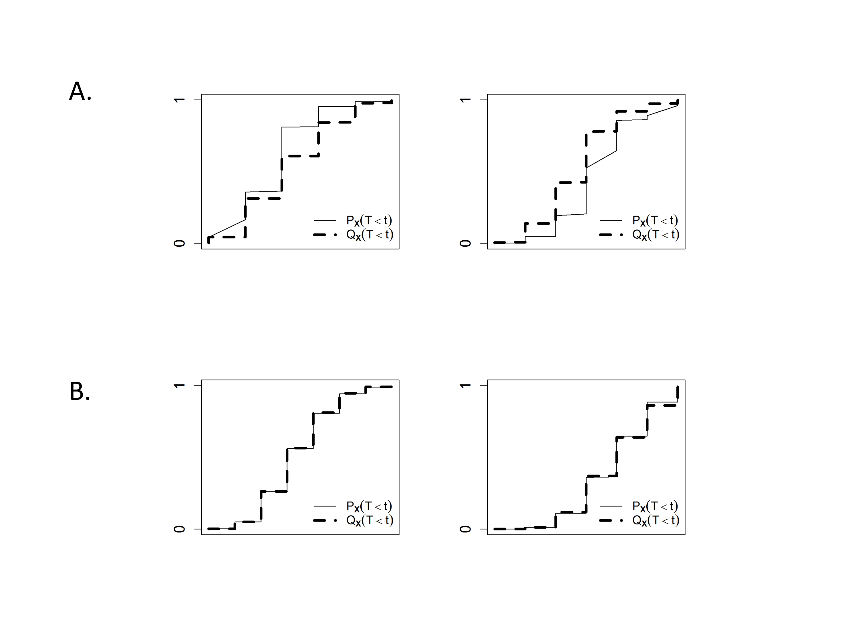
Figure 1: Illustration of Resampling Distributions. Empirical cumulative distribution functions for simulated matrices $\bf X$ in which independent rows $\mbox{$\bf X$}_{i\cdot}$ are generated by a first-order finite-state Markov chain. Each panel corresponds to a simulated $4\times m$ matrix $\bf X$ with $m=10$ (A) or $m=50$ (B).

3 Application to Genomic Data

In tumor studies DNA copy number values for each subject are measured with respect to a normal reference, typically either a paired normal sample or a pooled reference. In the autosomes the normal DNA copy number is two. Underlying genomic instability in tumor tissue can result in DNA copy number gains and losses, and often these changes lead to increased or decreased expression, respectively, of affected genes (Pinkel and Albertson 2005). Some of these genetic aberrations occur at random locations throughout the genome, and these are termed sporadic. In contrast, recurrent aberrations are found in the same genomic region in multiple subjects. It is believed that recurrent aberrations arise because they lead to changes in gene expression that provide a selective growth advantage. Therefore regions containing recurrent aberrations are of interest because they may harbor genes associated with the tumor phenotype. Distinguishing sporadic and recurrent aberrations is largely a statistical issue, and the cyclic shift procedure was designed to perform this task.

DNA methylation values for a given subject are also measured with respect to a paired or pooled normal reference. Although DNA methylation values are not constant across the genome, even in normal tissue, at a fixed location they are quite stable in normal samples from a given tissue type. Epigenetic instability can disrupt normal methylation patterns, leading to methylation gains and losses, and these changes can affect gene expression levels (Laird 2003). Regions of the genome that exhibit recurrent hyper- or hypo-methylation in tumor tissue are of interest.

3.1 Peeling

In many applications more than one atypical marker may be present, and as a result multiple columns may produce summary statistics with extreme values. In tumor tissue, for example, underlying genomic instability can result in gains and losses of multiple chromosomal regions; likewise, epigenetic instability can lead to aberrant patterns of DNA methylation throughout the genome. In order to identify multiple atypical markers and assess their statistical significance it is necessary to remove the effect of each discovered marker before initiating a search for the next marker. This task is carried out by a process known as peeling. Several peeling procedures have been proposed in the literature, including those employed by GISTIC (Beroukhim et al. 2007) and DiNAMIC (Walter et al. 2011). In the applications here we make use of the procedure described in detail in Walter et al. (2011) .

3.2 DNA Copy Number Data

Walter et al. (2011) used the cyclic shift procedure to analyze the Wilms’ tumor data of Natrajan et al. (2006). Here we apply the procedure to the lung adenocarcinoma dataset of Chitale et al. (2009), with $n$ = 192 and $m$ = 40478. We detected a number of highly significant findings under the null hypothesis that no recurrent copy number gains or losses are present. Table 1 lists the genomic positions of the the three most significant copy number gains and losses, as well as neighboring genes, most of which are known oncogenes and tumor suppressors. Strikingly, Weir et al. (2007) detected highly significant gains of the oncogenes TERT, ARNT, and MYC in their comprehensive investigation of the disease, each of which appears in Table 1. The loss results for chromsomes 8 and 9 in Table 1 are also highly concordant with previous findings of Weir et al. (2007), and Wistuba et al. (1999). Weir et al. (2007) detected chromosomal loss in a broad region of 13q that contains the locus in Table 1, but it is not clear if the target of this region is the known tumor-suppressor RB1 or some other gene.

Table 1: Genomic locations of the three most significant DNA copy number gains (top table) and losses (bottom table) found by applying the cyclic shift procedure to the lung adenocarcinoma dataset of Chitale et al. (2009).

Chromosome	Gain Locus (bp)	Gene
5p15	967984	TERT
1q21	149346163	ARNT
8q24	128816933	MYC

Chromosome	Loss Locus (bp)	Gene
8p23	2795183	CSMD1
13q11	19254995	PSPC1
9p21	21958070	CDKN2A

3.3 DNA Methylation Data

Using unsupervised clustering techniques, Fackler et al. (2011) found an association between methylation patterns and estrogen-receptor status in a cohort of breast cancer tumors. This cohort consisted of 20 tumor/normal pairs, and we used differences in methylation signal between tumor and normal tissue as the observations. We applied the cyclic shift procedure to the resulting differences to detect loci that exhibited recurrent hyper- or hypomethylation in tumors. As shown in Table 2, the most significant hypermethylation sites occur in ABCA3, GALR1, and NID2, and these genes have previously been found to be highly methylated in lung adenocarcinoma, head and neck squamous cell carcioma, and bladder cancer, respectively, by Selamat et al. (2012), Misawa et al. (2008), and Renard et al. (2009). Hypomethylation of the transcription factor MYT1 on chromosome 20 was detected; this is notable because Viré et al. (2006) found that MYT1 could be activated via decreased methylation.

Table 2: Genomic locations of the three most significant hypermethylation (top table) and hypomethylation (bottom table) sites found by applying the cyclic shift procedure to the breast cancer dataset of Fackler et al. (2011).

Chromosome	Gain Locus (bp)	Gene
16p13	2331829	ABCA3
18q23	73091357	GALR1
14q22	51605897	NID2

Chromosome	Gain Locus (bp)	Gene
20q13	62266251	MYT1
3q24	144378065	SLC9A9
1q21	150565702	MCL1

3.4 Meta-Analysis of Genomewide Association Studies

Genome-wide association studies (GWAS) are used to identify genetic markers, typically single nucleotide polymorphisms (SNPs), that are associated with a disease of interest. When conducting a GWAS involving a common disease and alleles with small to moderate effect sizes, large numbers of cases and controls are required to have adequate power to detect disease SNPs (Pfeiffer et al. 2009).

The Welcome Trust Case Control Consortium (WTCCC 2007) performed a genome-wide association study of seven common familial diseases - bipolar disorder (BD), coronary artery disease (CAD), Crohn’s disease (CD), hypertension (HT), rheumatoid arthritis (RA), type I diabetes (T1D), and type II diabetes (T2D) - based on an analysis of 2000 separate cases for each disease and a set of 3000 controls. We applied the inverse of the standard normal cumulative distribution function to the Cochran-Armitrage trend test $p$-values from the WTCCC study, a transformation that produces z-scores whose values are similar those exhibited by a stationary process. We then analyzed the matrix $\bf X$ whose entries are negative thresholded z-scores arranged in rows corresponding to the seven disease phenotypes. As seen in Figure 2, a number of regional markers on chromosome 6 produce extremely large column sums. These markers lie in the major histocompatability complex (MHC), which is noteworthy because MHC class II genes have been shown to be associated with autoimmune disorders, including RA and T1D (Fernando et al. 2008). When applied to $\bf X$, cyclic shift testing identified several highly significant apparently pleiotropic SNPs in the MHC region that produced large entries in the rows corresponding to both RA and T1D, including rs9270986, which is upstream of the RA and T1D susceptibility gene HLA-DRB1.

The WTCCC dataset serves as a proof of principle for cyclic shift applied to GWAS studies, although the use of a common set of controls may create modest additional correlation not fully captured in the cyclic shifts. We note that the cyclic shift procedure appplied to GWAS is sensitive only to small $p$-values that occur in multiple studies. Thus the procedure is qualitatively different from typical meta-analyses, such as Zeggini et al. (2008), which can be sensitive to large observed effects form a single study.

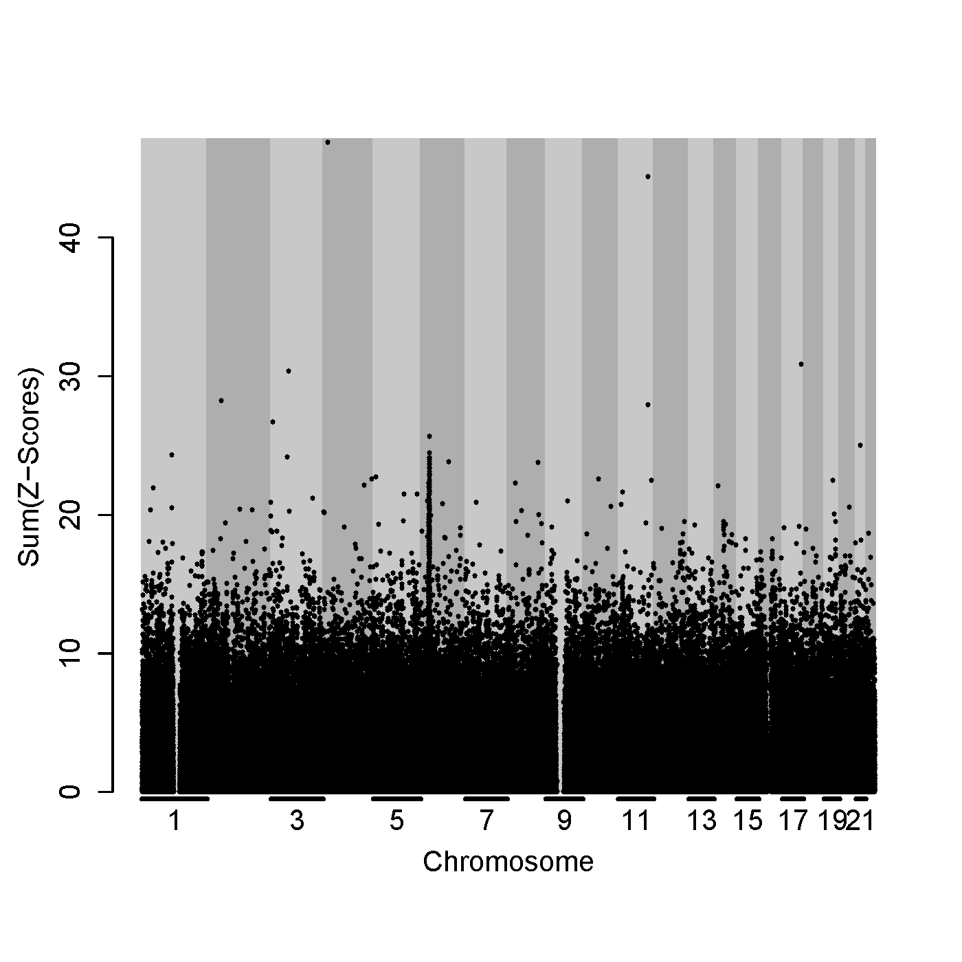
Figure 2: Cyclic Shift Testing Identifies Pleiotropic Single Nucleotide Polymorphisms. Marker-specific summary statistics were obtained from the Welcome Trust Case Control Consortium study and plotted genome-wide. Numerous regional markers in the multihistocompatability complex region of chromosome 6 exhibit large summary statistics, including several markers that were highly significant under cyclic shift testing and were associated with multiple disease phenotypes.

4 Proof of Theorem 1

Let $\bf X$ be a random $n\times m$ matrix whose rows $\mbox{$\bf X$}_{1\cdot},\dots,\mbox{$\bf X$}_{n\cdot}$ are independent realizations of a first-order stationary ergodic Markov chain with countable state space ${\cal{A}}$. Denote the distribution of $\bf X$ in ${\cal A}^{n\times m}$ by $P_{m}$. Let $p_{1}(\cdot)$ and $p(\cdot|\cdot)$ denote, respectively, the stationary distribution and the one-step transition probability of the Markov chain defining the rows of $\bf X$. Let $p_{l}(\cdot)$ denote the joint probability mass function of $l$ contiguous variables in the chain. Thus the vectors $\mbox{$\bf X$}_{i\cdot}$ have common probability mass function

$$p_{m}(x_{0},\dots,x_{m-1})\ =\ p_{1}(x_{0})\prod_{j=1}^{m-1}p(x_{j}|x_{j-1}).$$ (4.1)

In what follows we assume that (2.2) holds. The ergodicity assumption on the Markov chain ensures that the joint probability mass function of $(X_{0},X_{m-1})$ converges to the joint probability mass function of the pair $(X,X^{\prime})$ where $X,X^{\prime}\in{\cal A}$ are independent with the same distribution as $X_{0}$. It follows that

$$\frac{p_{1}(X_{i,0})\,p_{1}(X_{i,m-1})}{p_{2}(X_{i,0},X_{i,m-1})}\ =\ O_{P}(1)\ \ 1\leq i\leq n.$$ (4.2)

In other words, for each row $i$ the ratio in (4.2) is stochastically bounded under $P_{m}$ as $m$ tends to infinity.

Suppose for the moment that $m$ is fixed. For any integer $r$, define the cyclic shift $\sigma_{r}:{\cal A}^{m}\to{\cal A}^{m}$ on sequences of length $m$ by

$$\sigma_{r}(x_{0},x_{1},\dots,x_{m-1})=(x_{[r]},x_{[r+1]},\dots,x_{[r+(m-1)]})$$

where $[k]=k\mbox{ mod }m$. We index vectors as $(x_{0},x_{1},\dots,x_{m-1})$ rather than $(x_{1},x_{2},\dots,x_{m})$, as was done in the body of the present manuscript, because this allows us to write the subscripts of the shifted vector in terms of $[k]$, substantially reducing notation. For each $\mbox{$\bf r$}=(r_{1},\dots,r_{n})\in{\mathbb{Z}}^{n}$ define $\sigma_{\mbox{\scriptsize\bf r}}(\mbox{$\bf X$})$ to be the $n\times m$ matrix with rows $\sigma_{r_{1}}(\mbox{$\bf X$}_{1\cdot}),\dots,\sigma_{r_{n}}(\mbox{$\bf X$}_{n\cdot})$. If ${\mbox{$\bf r$}},{\mbox{$\bf s$}}\in{\mathbb{Z}}^{n}$, then it is easy to verify that

$$(\sigma_{\mbox{\scriptsize\bf r}}\circ\sigma_{\mbox{\scriptsize\bf s}})(\mbox{$\bf X$})\ =\ (\sigma_{\mbox{\scriptsize\bf s}}\circ\sigma_{\mbox{\scriptsize\bf r}})(\mbox{$\bf X$})\ =\ (\sigma_{{\mbox{\scriptsize\bf r}}+{\mbox{\scriptsize\bf s}}})(\mbox{$\bf X$}).$$

Let ${\cal S}_{m}(\mbox{$\bf X$})=\{\sigma_{\mbox{\scriptsize\bf r}}(\mbox{$\bf X$}):\mbox{$\bf r$}\in\mathbb{Z}^{n}\}$ be the set of cyclic shifts of $\bf X$.

Let $P_{\mbox{\scriptsize\bf X}}$ and $Q_{\mbox{\scriptsize\bf X}}$ be the true conditional and cyclic conditional distributions given ${\cal S}_{m}(\mbox{$\bf X$})$, defined by $P_{\mbox{\scriptsize\bf X}}(A)=P_{m}(A\,|\,{\cal S}_{m}(\mbox{$\bf X$}))$ and $Q_{\mbox{\scriptsize\bf X}}(A)=m^{-n}\,|A\cap{\cal S}_{m}(\mbox{$\bf X$})|$, respectively. In order to compare the distributions $P_{\mbox{\scriptsize\bf X}}$ and $Q_{\mbox{\scriptsize\bf X}}$ we introduce two closely related distributions, $P_{\mbox{\scriptsize\bf X}}^{o}$ and $Q_{\mbox{\scriptsize\bf X}}^{o}$, that are more amenable to analysis. Let $P_{\mbox{\scriptsize\bf X}}^{o}$ be a (random) measure on ${\cal{A}}^{n\times m}$ defined by

$$P_{\mbox{\scriptsize\bf X}}^{o}(A)\ =\ \sum_{{\mbox{\scriptsize\bf r}}\in[m]^{n}}\eta(\sigma_{\mbox{\scriptsize\bf r}}(\mbox{$\bf X$}))\,I(\sigma_{\mbox{\scriptsize\bf r}}(\mbox{$\bf X$})\in A),$$

where $[m]=\{0,1,\ldots,m-1\}$ and

$$\eta(\sigma_{\mbox{\scriptsize\bf r}}(\mbox{$\bf X$}))\ =\ \prod_{i=1}^{n}\left[\frac{p_{m}(\sigma_{r_{i}}(\mbox{$\bf X$}_{i\cdot}))}{\sum_{s\in[m]}p_{m}(\sigma_{s}(\mbox{$\bf X$}_{i\cdot}))}\right].$$

Let $Q_{\mbox{\scriptsize\bf X}}^{o}$ be a (random) measure on ${\cal{A}}^{n\times m}$ defined by

$$Q_{\mbox{\scriptsize\bf X}}^{o}(A)\ =\ \sum_{{\mbox{\scriptsize\bf r}}\in[m]^{n}}\frac{1}{m^{n}}\,I(\sigma_{\mbox{\scriptsize\bf r}}(\mbox{$\bf X$})\in A).$$

One may readily verify that $P_{\mbox{\scriptsize\bf X}}^{o}({\cal{A}}^{m\times n})=Q_{\mbox{\scriptsize\bf X}}^{o}({\cal{A}}^{m\times n})=1$, so both $P_{\mbox{\scriptsize\bf X}}^{o}$ and $Q_{\mbox{\scriptsize\bf X}}^{o}$ are valid probability measures on ${\cal{A}}^{m\times n}$.

We will say that the set of cyclic shifts ${\cal{S}}_{m}(\mbox{$\bf X$})$ is full if its cardinality is equal to $m^{n}$, or equivalently, if all cyclic shifts of $\bf X$ are distinct.

Lemma 1.

If ${\cal{S}}_{m}(\mbox{$\bf X$})$ is full, then (a) $P_{\mbox{\scriptsize\bf X}}^{o}=P_{\mbox{\scriptsize\bf X}}$ and (b) $Q_{\mbox{\scriptsize\bf X}}^{o}=Q_{\mbox{\scriptsize\bf X}}$.

Proof.

(a) For any $A\subseteq{\cal{A}}^{n\times m}$ we may write $P_{\mbox{\scriptsize\bf X}}(A)$ as

$$\frac{P_{m}(A\cap{\cal{S}}_{m}(\mbox{\scriptsize\bf X}))}{P_{m}({\cal{S}}_{m}(\mbox{$\bf X$}))}=\sum_{{\mbox{\scriptsize\bf r}}\in[m]^{n}}\frac{P_{m}(\sigma_{\mbox{\scriptsize\bf r}}(\mbox{$\bf X$}))}{P_{m}({\cal{S}}_{m}(\mbox{$\bf X$}))}I(\sigma_{\mbox{\scriptsize\bf r}}(\mbox{$\bf X$})\in A).$$ (4.3)

Since ${\cal{S}}_{m}(\mbox{$\bf X$})$ is full,

$$P_{m}({\cal{S}}_{m}(\mbox{$\bf X$}))=P_{m}\left(\bigcup_{{\mbox{\scriptsize\bf r}}\in[m]^{n}}\sigma_{\mbox{\scriptsize\bf r}}(\mbox{$\bf X$})\right)=\sum_{{\mbox{\scriptsize\bf r}}\in[m]^{n}}P_{m}(\sigma_{\mbox{\scriptsize\bf r}}(\mbox{$\bf X$})).$$

The independence of the rows of $\bf X$ allows us to write the last expression as $\displaystyle{\sum_{\mbox{\scriptsize\bf r}\in[m]^{n}}\prod_{i=1}^{n}p_{m}(\sigma_{r_{i}}(\mbox{$\bf X$}_{i\cdot}))}$, but this may be rewritten as $\displaystyle{\prod_{i=1}^{n}\sum_{s\in[m]}p_{m}(\sigma_{s}(\mbox{$\bf X$}_{i\cdot}))}$. Therefore (4.3) is equivalent to

$$\sum_{{\mbox{\scriptsize\bf r}}\in[m]^{n}}\left[\prod_{i=1}^{n}\frac{p_{m}(\sigma_{r_{i}}(\mbox{$\bf X$}_{i\cdot}))}{\sum_{s\in[m]}p_{m}(\sigma_{s}(\mbox{$\bf X$}_{i\cdot}))}\right]I(\sigma_{\mbox{\scriptsize\bf r}}(\mbox{$\bf X$})\in A)=P_{\mbox{\scriptsize\bf X}}^{o}(A).$$

(b) There are $m^{n}$ elements in ${\cal{S}}_{m}(\mbox{$\bf X$})$ when $\bf X$ is full, so for any $A\in\cal{A}$

$$Q_{\mbox{\scriptsize\bf X}}(A)=m^{-n}\,|A\cap{\cal S}_{m}(\mbox{$\bf X$})|=\sum_{{\mbox{\scriptsize\bf r}}\in[m]^{n}}\frac{1}{m^{n}}\,I(\sigma_{\mbox{\scriptsize\bf r}}(\mbox{$\bf X$})\in A)=Q_{\mbox{\scriptsize\bf X}}^{o}(A).$$

∎

Lemma 2.

Let $\mathrm{\mathbf{x}}=(x_{0},x_{1},\dots,x_{m-1})\in{\cal{A}}^{m}$ be a sequence of length $m$. Let $k$ be the least positive integer such that $\sigma_{k}(\mathrm{\mathbf{x}})=\mathrm{\mathbf{x}}$. If $k<m$, then $k$ divides $m$, and $\mathrm{\mathbf{x}}$ is equal to the repeated concatenation of a fixed block of length $k$.

Proof.

Suppose to the contrary that $1\leq k<m$ does not divide $m$. Then we may write $m=kq+r$, where $1\leq r<k$. Now $\sigma_{k}({\mbox{$\bf x$}})={\mbox{$\bf x$}}$ implies that $\sigma_{-k}({\mbox{$\bf x$}})={\mbox{$\bf x$}}$, and it follows that

$$\sigma_{r}({\mbox{$\bf x$}})=\sigma_{m-kq}({\mbox{$\bf x$}})=\sigma_{m}\circ\sigma_{-kq}({\mbox{$\bf x$}})={\mbox{$\bf x$}}.$$

As this contradicts the minimality of $k$, we conclude that $k$ divides $m$. The second conclusion follows in a straightforward way from the first. ∎

Corollary 1.

If $\mathrm{\mathbf{x}}\in{\cal{A}}^{m}$ is such that $\sigma_{k}(\mathrm{\mathbf{x}})=\mathrm{\mathbf{x}}$ for some $1\leq k<m$, then $\mathrm{\mathbf{x}}$ contains two disjoint, equal blocks of length at least $m/3$.

Lemma 3.

If (2.2) holds, then $P_{m}({\cal{S}}_{m}(\mathrm{\mathbf{X}})\ \text{is full})$ converges to 1 as $m$ tends to infinity.

Proof.

We begin by noting that ${\cal{S}}_{m}(\mbox{$\bf X$})$ is full if ${\cal{S}}_{m}(\mbox{$\bf X$}_{i\cdot})$ is full for $i=1,\ldots,n$. Because the rows of $\bf X$ are independent, it therefore suffices to prove the result in the case $n=1$. Thus we write $\mbox{$\bf X$}=(X_{0},\dots,X_{m-1})$. If ${\cal{S}}_{m}(\mbox{$\bf X$})$ is not full, then Corollary 1 implies that there exist integers $l,r\geq m/3$ such that $X_{j}=X_{r+j}$ for $j=0,\ldots,l-1$. An easy calculation using the Markov property shows that, for fixed $r$, the $P_{m}$-probability of this event is at most $\rho^{l-1}$, where $\rho<1$ is the maximum appearing in (2.2). Thus the probability that ${\cal{S}}_{m}(\mbox{$\bf X$})$ is not full is at most $m\,\rho^{m/3-1}$, which tends to zero as $m$ tends to infinity. ∎

Definition: A set $A\subset{\cal{A}}^{n\times m}$ is invariant under constant shifts if $\sigma_{\mbox{\scriptsize\bf r}}(A)=A$ whenever $\mbox{$\bf r$}=(r,\ldots,r)$ is a constant index sequence. Let $\mathbb{A}_{m}$ be the family of all sets $A\subset{\cal{A}}^{n\times m}$ that are invariant under constant shifts.

Theorem 2.

Suppose that (2.2) holds and that the stationary Markov chain described by (4.1) is ergodic. Then

$$\max_{A\in\mathbb{A}_{m}}|P_{\mbox{\scriptsize\bf X}}^{o}(A)-Q_{\mbox{\scriptsize\bf X}}^{o}(A)|\ \to\ 0$$

in probability as $m$ tends to infinity.

Proof.

Fix $m\geq 1$ and $A\in\mathbb{A}_{m}$. For $k\in{\mathbb{Z}}$ let ${\mbox{$\bf k$}}^{\ast}=(k,k,\dots,k)\in{\mathbb{Z}}^{n}$ be the constant sequence each of whose coordinates is equal to $k$. It follows from the invariance of $A$ and the basic properties of cyclic shifts that for each $k\in{\mathbb{Z}}$,

$$P_{\mbox{\scriptsize\bf X}}^{o}(A) = \sum_{{\mbox{\scriptsize\bf r}}\in[m]^{n}}\eta(\sigma_{\mbox{\scriptsize\bf r}}(\mbox{$\bf X$}))\,I(\sigma_{\mbox{\scriptsize\bf r}}(\mbox{$\bf X$})\in A)$$

$$= \sum_{{\mbox{\scriptsize\bf r}}\in[m]^{n}}\eta(\sigma_{\mbox{\scriptsize\bf r}+\mbox{\scriptsize\bf k}^{*}}(\mbox{$\bf X$}))\,I(\sigma_{\mbox{\scriptsize\bf r}+\mbox{\scriptsize\bf k}^{*}}(\mbox{$\bf X$})\in A)$$

$$= \sum_{{\mbox{\scriptsize\bf r}}\in[m]^{n}}\eta(\sigma_{\mbox{\scriptsize\bf r}+\mbox{\scriptsize\bf k}^{*}}(\mbox{$\bf X$}))\,I(\sigma_{\mbox{\scriptsize\bf r}}(\mbox{$\bf X$})\in A).$$

Thus we may express $P_{\mbox{\scriptsize\bf X}}^{o}(A)$ in the form of an average over $k$:

$$P_{\mbox{\scriptsize\bf X}}^{o}(A)\ =\ \sum_{{\mbox{\scriptsize\bf r}}\in[m]^{n}}\left[\frac{1}{m}\sum_{k\in[m]}\eta(\sigma_{\mbox{\scriptsize\bf r}+\mbox{\scriptsize\bf k}^{*}}(\mbox{$\bf X$}))\right]I(\sigma_{\mbox{\scriptsize\bf r}}(\mbox{$\bf X$})\in A).$$

Combining this last expression with the definition of $Q_{\mbox{\scriptsize\bf X}}^{o}$ yields the bound

$$|P_{\mbox{\scriptsize\bf X}}^{o}(A)-Q_{\mbox{\scriptsize\bf X}}^{o}(A)| \leq \sum_{{\mbox{\scriptsize\bf r}}\in[m]^{n}}\left|\frac{1}{m}\sum_{k\in[m]}\eta(\sigma_{\mbox{\scriptsize\bf r}+\mbox{\scriptsize\bf k}^{*}}(\mbox{$\bf X$}))-\frac{1}{m^{n}}\,\right|I(\sigma_{\mbox{\scriptsize\bf r}}(\mbox{$\bf X$})\in A)$$ (4.4)

$$\leq \sum_{{\mbox{\scriptsize\bf r}}\in[m]^{n}}\left|\frac{1}{m}\sum_{k\in[m]}\eta(\sigma_{\mbox{\scriptsize\bf r}+\mbox{\scriptsize\bf k}^{*}}(\mbox{$\bf X$}))-\frac{1}{m^{n}}\,\right|$$

$$= \frac{1}{m^{n}}\sum_{{\mbox{\scriptsize\bf r}}\in[m]^{n}}\left|\frac{1}{m}\sum_{k\in[m]}m^{n}\eta(\sigma_{\mbox{\scriptsize\bf r}+\mbox{\scriptsize\bf k}^{*}}(\mbox{$\bf X$}))-1\,\right|.$$

We now turn our attention to the quantity $m^{n}\,\eta(\sigma_{\mbox{\scriptsize\bf r}+\mbox{\scriptsize\bf k}^{*}}(\mbox{$\bf X$}))$ appearing in (4.4). Let $\mbox{$\bf x$}=(x_{0},\dots,x_{m-1})$ be a fixed $m$-vector with entries in ${\cal{A}}$, and let $t\in{\mathbb{Z}}$. By expanding the joint probability $p_{m}(\cdot)$ as a product of one-step conditional probabilities and canceling common terms, a straightforward calculation shows that for all integers $t$

$$m\cdot\frac{p_{m}(\sigma_{t}(\mbox{$\bf x$}))}{\sum_{s\in[m]}p_{m}(\sigma_{s}(\mbox{$\bf x$}))}\ =\ \rho_{t}(\mbox{$\bf x$})\,\gamma_{m}^{-1}(\mbox{$\bf x$})$$ (4.5)

where

$$\rho_{t}(\mbox{$\bf x$})=\frac{p_{1}(x_{[t]})\,p_{1}(x_{[t-1]})}{p_{2}(x_{[t]},x_{[t-1]})}\ \mbox{ and }\ \gamma_{m}(\mbox{$\bf x$})\,=\,\frac{1}{m}\sum_{j=0}^{m-1}\rho_{j}(\mbox{$\bf x$}).$$

(Recall that $[t]=t\ {\text{mod}}\ m$.) It follows from the definition of $\eta(\mbox{$\bf X$})$ and equation (4.5) that

$$m^{n}\,\eta(\sigma_{\mbox{\scriptsize\bf r}+\mbox{\scriptsize\bf k}^{*}}(\mbox{$\bf X$})) = \prod_{i=1}^{n}\left[\frac{m\,p_{m}(\sigma_{r_{i}+k}(\mbox{$\bf X$}_{i\cdot}))}{\sum_{s\in[m]}p_{m}(\sigma_{s}(\mbox{$\bf X$}_{i\cdot}))}\right]$$

$$= \prod_{i=1}^{n}\rho_{r_{i}+k}(\mbox{$\bf X$}_{i\cdot})\,\gamma_{m}^{-1}(\mbox{$\bf X$}_{i\cdot})\ =\ \Gamma_{m}^{-1}(\mbox{$\bf X$})\,\prod_{i=1}^{n}\rho_{r_{i}+k}(\mbox{$\bf X$}_{i\cdot})$$

where $\Gamma_{m}(\mbox{$\bf X$})=\prod_{i=1}^{n}\gamma_{m}(\mbox{$\bf X$}_{i\cdot})$.

The assumptions of the theorem ensure that the random variables $X_{i,0}$, …, $X_{i,m-1}$ in the $i$th row of $\bf X$ are the initial terms of a stationary ergodic process, and therefore the same is true of the non-negative random variables $\rho_{1}(\mbox{$\bf X$}_{i\cdot})$,…,$\rho_{m-1}(\mbox{$\bf X$}_{i\cdot})$. Note that the random variable $\rho_{0}(\mbox{$\bf X$}_{i\cdot})$ cannot be included in this sequence because it involves the non-adjacent variables $X_{i,0}$ and $X_{i,m-1}$. It is easy to see that

$$\mathbb{E}\rho_{1}(\mbox{$\bf X$}_{i\cdot})\ =\ \mathbb{E}\left(\frac{p_{1}(X_{i,1})\,p_{1}(X_{i,0})}{p_{2}(X_{i,0},X_{i,1})}\right)\ =\ \sum_{u,v\in{\cal{A}}}\frac{p(u)\,p(v)}{p(u,v)}\,p(u,v)\ =\ 1.$$

From the ergodic theorem and the fact that $\rho_{0}(\mbox{$\bf X$}_{i\cdot})$ is stochastically bounded (see (4.2)), it follows that

$$\gamma_{m}({\bf X}_{i\cdot})\ =\ \mathbb{E}\rho_{1}(\mbox{$\bf X$}_{i\cdot})+o_{P}(1)\ =\ 1+o_{P}(1),$$ (4.6)

and therefore $\Gamma_{m}(\mbox{$\bf X$})$ and $\Gamma_{m}^{-1}(\mbox{$\bf X$})$ are equal to $1+o_{P}(1)$ as well. (Here and in what follows the stochastic order symbols $o_{P}(1)$ and $O_{P}(1)$ refer to the underlying measure $P_{m}$ with $m$ tending to infinity). For $\mbox{$\bf r$}\in[m]^{n}$ let $V_{0}(\mbox{$\bf r$})=\{k\in[m]:r_{i}+k\equiv 0\mbox{ mod $m$ for some }1\leq i\leq n\}$ and let $V_{1}(\mbox{$\bf r$})=[m]\setminus V_{0}(\mbox{$\bf r$})$. Note that $|V_{0}(\mbox{$\bf r$})|\leq n$ for each $\mbox{$\bf r$}\in[m]^{n}$. Combining the relation (4.6) with inequality (4.4) and equation (4.5), we conclude that

$$|P_{X}^{o}(A)-Q_{X}^{o}(A)|$$ (4.7)

$$\leq \Gamma_{m}^{-1}(\mbox{$\bf X$})\cdot\frac{1}{m^{n}}\sum_{{\mbox{\scriptsize\bf r}}\in[m]^{n}}\left|\frac{1}{m}\sum_{k\in[m]}\,\prod_{i=1}^{n}\rho_{r_{i}+k}(\mbox{$\bf X$}_{i\cdot})-1\,\right|\ +\ |\Gamma_{m}^{-1}(\mbox{$\bf X$})-1|$$

$$= O_{P}(1)\cdot\frac{1}{m^{n}}\sum_{{\mbox{\scriptsize\bf r}}\in[m]^{n}}\left|\frac{1}{m}\sum_{k\in[m]}\,\prod_{i=1}^{n}\rho_{r_{i}+k}(\mbox{$\bf X$}_{i\cdot})-1\,\right|\ +\ o_{P}(1)$$

$$= O_{P}(1)\cdot\frac{1}{m^{n}}\sum_{{\mbox{\scriptsize\bf r}}\in[m]^{n}}\left|\frac{1}{m}\sum_{k\in V_{1}({\mbox{\scriptsize\bf r}})}\,\prod_{i=1}^{n}\rho_{r_{i}+k}(\mbox{$\bf X$}_{i\cdot})-1\,\right|\ +\ O_{P}(1)\,\Delta_{m}\ +\ o_{P}(1)$$

where in the last line

$$\Delta_{m}\ :=\ \frac{1}{m^{n}}\sum_{{\mbox{\scriptsize\bf r}}\in[m]^{n}}\frac{1}{m}\sum_{k\in V_{0}({\mbox{\scriptsize\bf r}})}\,\prod_{i=1}^{n}\rho_{r_{i}+k}(\mbox{$\bf X$}_{i\cdot}).$$

As the upper bound in (4.7) is independent of our choice of $A\in\mathbb{A}_{m}$, it is enough to show that the first two terms in (4.7) are $o_{P}(1)$. Concerning the first term, by Markov’s inequality it suffices to show that

$$\max_{\mbox{\scriptsize\bf r}\in[m]^{n}}\mathbb{E}\left|\frac{1}{m}\sum_{k\in V_{1}({\mbox{\scriptsize\bf r}})}\prod_{i=1}^{n}\rho_{r_{i}+k^{\prime}}(\mbox{$\bf X$}_{i\cdot})-1\,\right|\ \to\ 0\ \mbox{ as }\ m\to\infty.$$

This follows from Corollary 2 below. As for the second term, note that

$$\Delta_{m} \leq \prod_{i=1}^{n}(\rho_{0}(\mbox{$\bf X$}_{i\cdot})\vee 1)\cdot\left[\frac{1}{m^{n}}\sum_{{\mbox{\scriptsize\bf r}}\in[m]^{n}}\frac{1}{m}\sum_{k\in V_{0}({\mbox{\scriptsize\bf r}})}\,\prod_{i:r_{i}+k\neq 0}\rho_{r_{i}+k}(\mbox{$\bf X$}_{i\cdot})\right]$$

$$= O_{P}(1)\cdot\left[\frac{1}{m^{n}}\sum_{{\mbox{\scriptsize\bf r}}\in[m]^{n}}\frac{1}{m}\sum_{k\in V_{0}(\mbox{\scriptsize\bf r})}\,\prod_{i:r_{i}+k\neq 0}\rho_{r_{i}+k}(\mbox{$\bf X$}_{i\cdot})\right]$$

The term in brackets is non-negative and has expectation at most $n/m$. Thus $\Delta_{m}=o_{P}(1)$ and the result follows. ∎

Let $\{U_{1}(k):k\geq 0\}$, …, $\{U_{n}(k):k\geq 0\}$ be independent, real-valued stationary ergodic processes defined on the same underlying probability space. Suppose that $\mathbb{E}|U_{i}(0)|$ is bounded for $i=1,\ldots,n$, and define $\mu=\Pi_{i=1}^{n}\mathbb{E}(U_{i}(0))$. Let ${\bf r}=(r_{1},\ldots,r_{n})$ denote a vector with non-negative integer-valued components. For $k,m\geq 1$ define random variables

$$V_{m}(k:{\bf r})\ =\ \prod_{i=1}^{n}U_{i}((r_{i}+k)\,\mbox{mod}\,m)-\mu.$$

The independence of the processes $\{U_{i}(\cdot)\}$ ensures that $\mathbb{E}(V_{m}(k:{\bf r}))=0$.

Lemma 4.

Under the assumptions above, $\max_{{\bf r}\in{\mathbb{Z}}^{n}}\,\mathbb{E}\left|m^{-1}\sum_{k=0}^{m-1}V_{m}(k:{\bf r})\right|$ converges to zero as $m$ tends to infinity.

Proof.

Standard arguments show that the joint process $\{(U_{1}(k),\ldots,U_{n}(k)):k\geq 0\}$ is stationary and ergodic, and therefore the same is true for the process $\{\prod_{i=1}^{n}U_{i}(k):k\geq 0\}$ of products. The $L_{1}$ ergodic theorem implies that

$$\Delta(l)\ =\ \mathbb{E}\left|\,\frac{1}{l}\sum_{k=0}^{l-1}\left(\prod_{i=1}^{n}U_{i}(k)\,-\,\mu\right)\right|\ \to\ 0\ \mbox{ as }\ l\to\infty.$$ (4.8)

Note also that

$$\Delta(l)\ \leq\ \mathbb{E}\left|\,\prod_{i=1}^{n}U_{i}(0)\,-\,\mu\,\right|\ \leq\ 2\prod_{i=1}^{n}\mathbb{E}|U_{i}(0)|\ \stackrel{{\scriptstyle\scriptscriptstyle\triangle}}{{=}}\ \Delta_{0}$$ (4.9)

which is bounded by assumption.

Fix $m\geq 1$ and ${\bf r}=(r_{1},\ldots,r_{n})$ with $r_{i}\geq 0$. Because the indices of $U_{i}(\cdot)$ in $V_{m}(k:{\bf r})$ are assessed modulo $m$, we may assume without loss of generality that $0\leq r_{1},\ldots,r_{n}\leq m-1$. Let $0\leq r(1)<r(2)<\cdots<r(n^{\prime})\leq m-1$ be the distinct order statistics of $r_{1},\ldots,r_{n}$, and note that $n^{\prime}\leq n$. Define $r(0)=0$, $r(n^{\prime}+1)=m$, and the differences $m_{j}=r(j+1)-r(j)$ for $j=0,\ldots,n^{\prime}$. Consider the decomposition

$$\sum_{k=0}^{m-1}V_{m}(k:{\bf r})\ =\ \sum_{j=0}^{n^{\prime}}W_{j}\ \mbox{ where }\ W_{j}\ =\sum_{k=r(j)}^{r(j+1)-1}V_{m}(k:{\bf r}).$$ (4.10)

The key feature of the sum $W_{j}$ is this: for $r(j)\leq k\leq r(j+1)-1$ there are no “breaks” in the indexing of the terms $U_{i}((r_{i}+k)\,\mbox{mod}\,m)$ in $V_{m}(k:{\bf r})$ arising from the modular sum. In particular, there exist integers $\tilde{r}_{1},\ldots,\tilde{r}_{n}$ such that $(r_{i}+k)\,\mbox{mod}\,m=\tilde{r}_{i}+k$ for each $i=1,\ldots,n$, and each $k$ in the sum defining $W_{j}$. As a result, the stationarity and independence of the individual processes $\{U_{i}(\cdot)\}$ ensures that $W_{j}$ is equal in distribution to the random variable

$$\tilde{W}_{j}\ =\ \sum_{k=0}^{m_{j}-1}\left(\prod_{i=1}^{n}U_{i}(k)\,-\,\mu\right).$$

We now turn our attention to the expectation in the statement of the lemma. It follows immediately from the decomposition (4.10) that

$$\frac{1}{m}\sum_{k=0}^{m-1}V_{m}(k:{\bf r})\ =\ \sum_{j=0}^{n^{\prime}}\frac{m_{j}}{m}\frac{1}{m_{j}}W_{j},$$

which yields the elementary bound

$$\left|\frac{1}{m}\sum_{k=0}^{m-1}V_{m}(k:{\bf r})\right|\ \leq\ \sum_{j=0}^{n^{\prime}}\frac{m_{j}}{m}\left|\frac{1}{m_{j}}W_{j}\right|.$$

Taking expectations of both sides in the last display yields the inequality

$$\mathbb{E}\left|\frac{1}{m}\sum_{k=0}^{m-1}V_{m}(k:{\bf r})\right|\ \leq\ \sum_{j=0}^{n^{\prime}}\frac{m_{j}}{m}\,\mathbb{E}\left|\frac{1}{m_{j}}W_{j}\right|\ =\ \sum_{j=0}^{n^{\prime}}\frac{m_{j}}{m}\,\mathbb{E}\left|\frac{1}{m_{j}}\tilde{W}_{j}\right|\ =\ \sum_{j=0}^{n^{\prime}}\frac{m_{j}}{m}\,\Delta(m_{j}),$$

where the first equality follows from the distributional equivalence of $W_{j}$ and $\tilde{W}_{j}$. In particular, for each integer $l\geq 1$ we have

$$\mathbb{E}\left|\frac{1}{m}\sum_{k=0}^{m-1}V_{m}(k:{\bf r})\right|\ \leq\ \sum_{j:m_{j}\leq l}\frac{m_{j}}{m}\,\Delta(m_{j})\,+\,\sum_{j:m_{j}>l}\frac{m_{j}}{m}\,\Delta(m_{j})\ \leq\ \frac{nl\Delta_{0}}{m}\,+\,\sup_{l^{\prime}>l}\Delta(l^{\prime}).$$

It follows from (4.8) and (4.9) that the final term in the last display tends to zero with $m$ if $l=l(m)$ is any sequence such that $l$ tends to infinity and $1/m$ converges to 0. Moreover, the final term does not depend on the vector $r$. This completes the proof of the lemma. ∎

An elementary argument using Lemma 4 establishes the following corollary.

Corollary 2.

Under the assumptions of Lemma 4, $\max_{r\in{\mathbb{N}}^{n}}\mathbb{E}\left|m^{-1}\sum_{k^{\prime}}V_{m}(k:r)\right|$ converges to zero as $m$ tends to infinity, where for each $r$ the sum is restricted to those $k^{\prime}\in[m]$ such that $r_{i}+k^{\prime}\not\equiv 0\mbox{ mod }m$.

Proof of Theorem 1: Theorem 1 follows from Theorem 2 and the fact that for each $B\subseteq\mathbb{R}$ the event $\{\mbox{$\bf Y$}:T_{m}(\mbox{$\bf Y$})\in B\}\in\mathbb{A}_{m}$ as $T_{m}$ is invariant under constant shifts.

5 Discussion

High resolution genomic data is routinely used by biomedical investigators to search for recurrent genomic aberrations that are associated with disease. Cyclic shift testing provides a simple, permutation based approach to identify aberrant markers in a variety of settings. Here we establish finite sample, large marker asymptotics for the consistency of $p$-values produced by cyclic shift testing. The results apply to a broad family of Markov based null distributions. To our knowledge, this is the first theoretical justification of a testing procedure of this kind. Although cyclic shift testing was developed for DNA copy number analysis, we demonstrate its utility for DNA methylation and meta-analysis of genome wide association studies.

6 Acknowledgements

This research was supported by the National Institutes of Health (T32 CA106209 for VW), the Environmental Protection Agency (RD835166 for FAW), the National Institutes of Health/National Institutes of Mental Health (1R01MH090936-01 for FAW), and the National Science Foundation (DMS-0907177 and DMS-1310002 for ABN).

7 Appendix

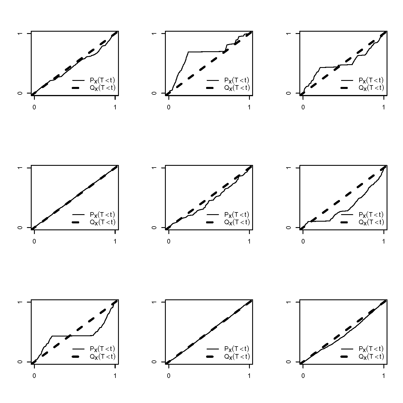
Figure A.1: Illustration of Resampling Distributions. Empirical cumulative distribution functions for simulated matrices $\bf X$ in which independent rows $\mbox{$\bf X$}_{i\cdot}$ are generated by a Gaussian AR(1) process with mean 0, standard deviation 1, and correlation .9. Each panel corresponds to a simulated $2\times 100$ matrix $\bf X$.

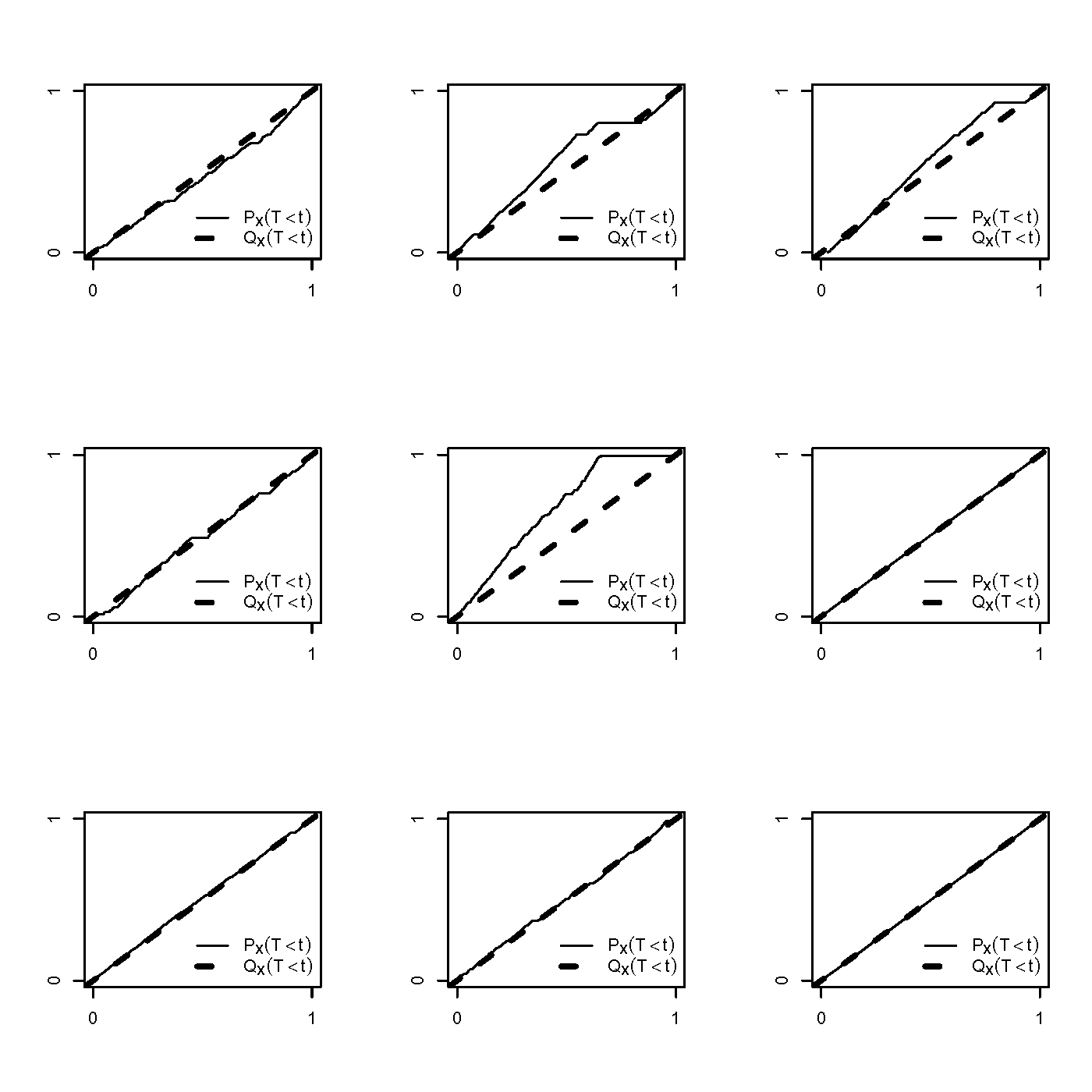
Figure A.2: Illustration of Resampling Distributions. Empirical cumulative distribution functions for simulated matrices $\bf X$ in which independent rows $\mbox{$\bf X$}_{i\cdot}$ are generated by a Gaussian AR(1) process with mean 0, standard deviation 1, and correlation .9. Each panel corresponds to a simulated $2\times 1000$ matrix $\bf X$.

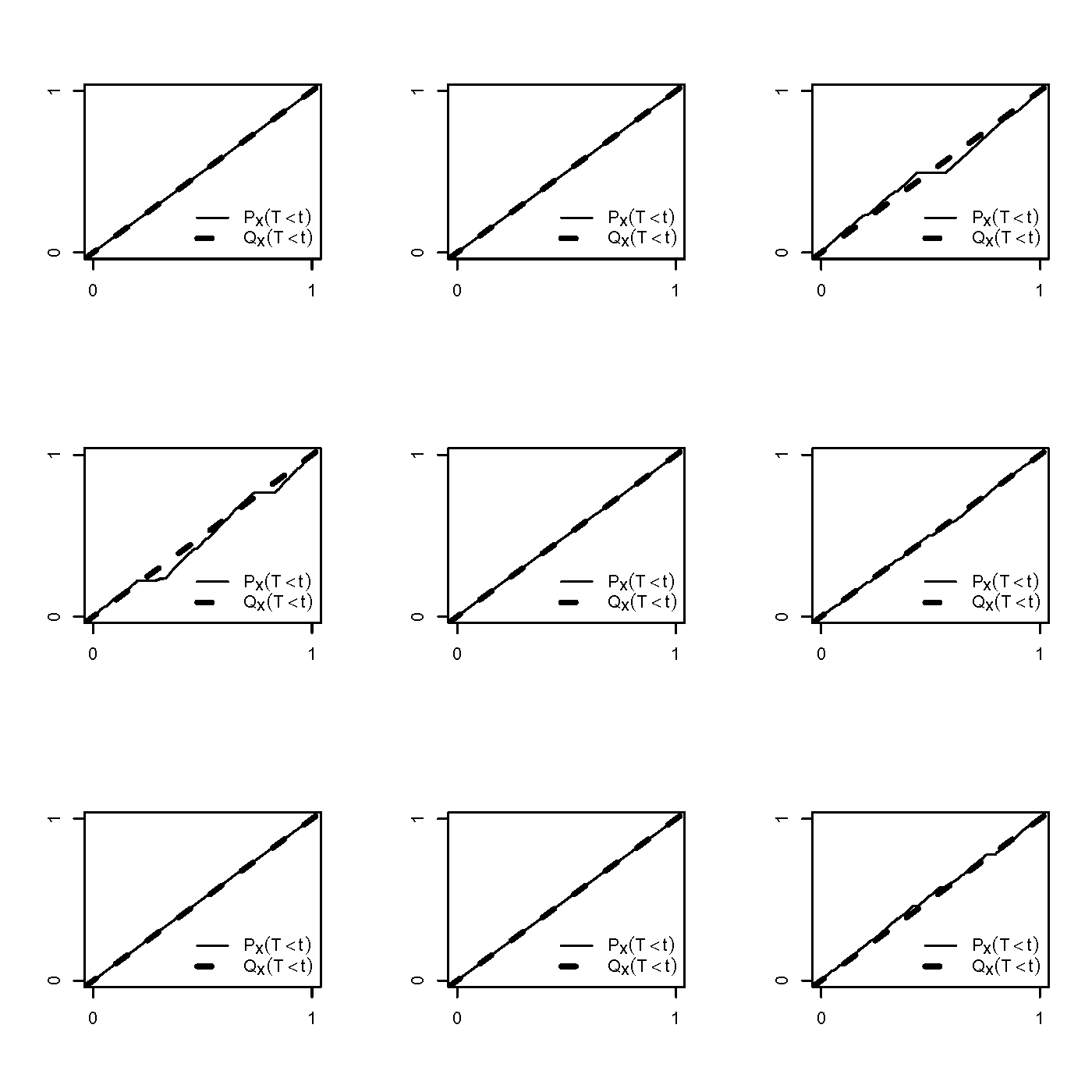
Figure A.3: Illustration of Resampling Distributions. Empirical cumulative distribution functions for simulated matrices $\bf X$ in which independent rows $\mbox{$\bf X$}_{i\cdot}$ are generated by a Gaussian AR(1) process with mean 0, standard deviation 1, and correlation .9. Each panel corresponds to a simulated $2\times 10000$ matrix $\bf X$.

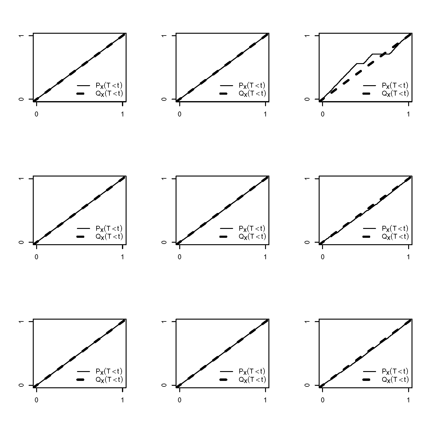
Figure A.4: Illustration of Resampling Distributions. Empirical cumulative distribution functions for simulated matrices $\bf X$ in which independent rows $\mbox{$\bf X$}_{i\cdot}$ are generated by a Gaussian AR(1) process with mean 0, standard deviation 1, and correlation .9. Each panel corresponds to a simulated $2\times 100000$ matrix $\bf X$.

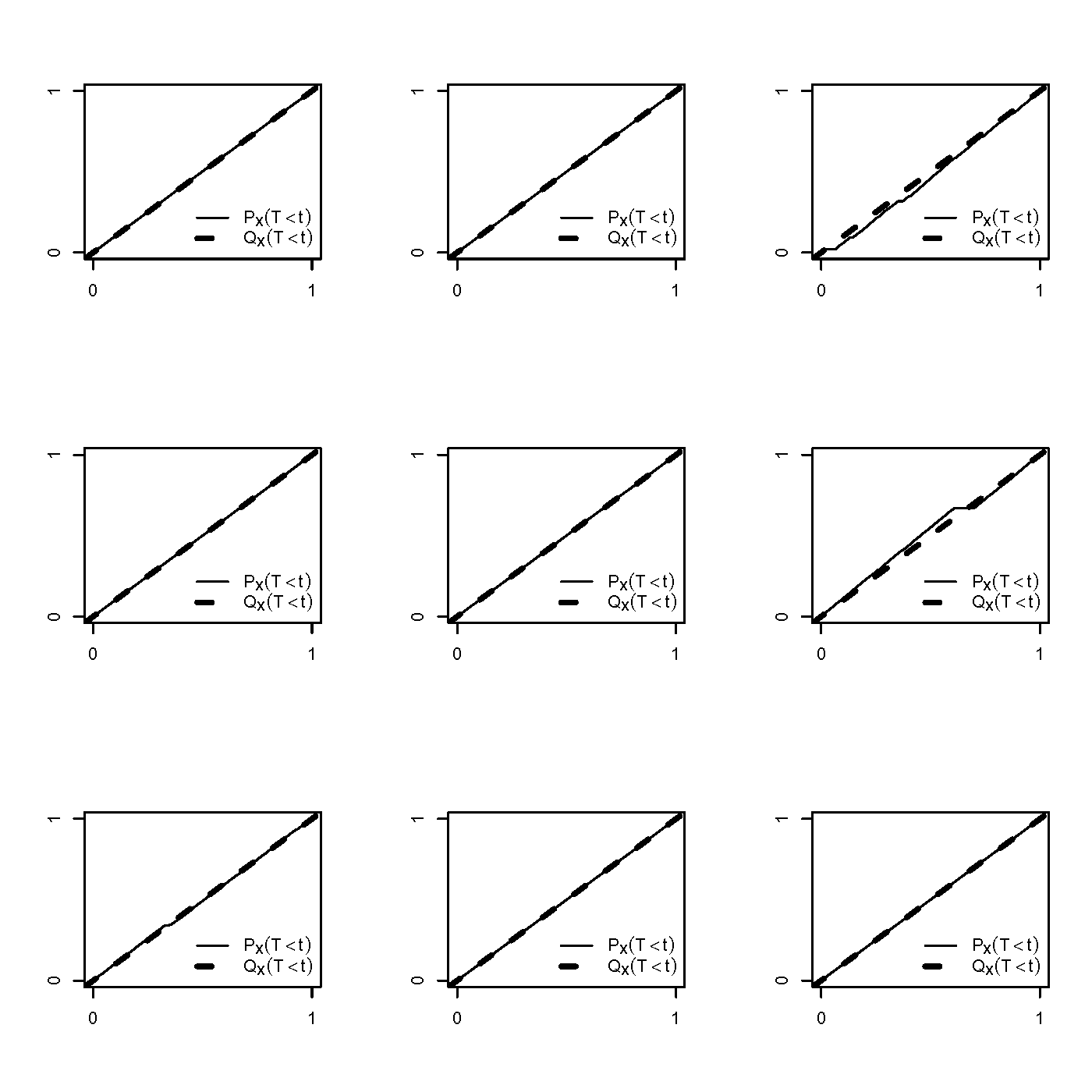
Figure A.5: Illustration of Resampling Distributions. Empirical cumulative distribution functions for simulated matrices $\bf X$ in which independent rows $\mbox{$\bf X$}_{i\cdot}$ are generated by a Gaussian AR(1) process with mean 0, standard deviation 1, and correlation .9. Each panel corresponds to a simulated $2\times 500000$ matrix $\bf X$.

References

- Beroukhim et al. [2007] Beroukhim, R., Getz, G., Nghlemphu, L., Barretina, J., Hsueh, T., Linhart, D., Vivanco, I., Lee, J.C., Huang, J.H., Alexander, S., et al. (2007). “Assessing the significance of chromosomal aberrations in cancer: Methodology and application to glioma,” Proc. Nat. Acad. Sci. 104 20007–20012.
- Chitale et al. [2009] Chitale, D., Gong, Y., Taylor, B.S., Broderick, S., Brennan, C., Somwar, R., Golas, B., Wang, L., Motoi, N., Szoke, J., et al. (2009). “An integrated genomic analysis of lung cancer reveals loss of DUSP4 in EGFR-mutant tumors,” Oncogene 28 2773–2783.
- Fackler et al. [2011] Fackler, M.J., Umbricht, C.B., Williams, D., Argani, P., Cruz, L-A., Merino, V.F., Teo, W.W., Zhang, Z., Huang, P., Visananthan, K., et al. (2011). “Genome-wide methylation analysis identifies genes specific to breast cancer hormone receptor status and risk of recurrence,” Cancer Res. 71 6195–6207.
- Fernando et al. [2008] Fernando, M.M.A., Stevens, C.R., Walsh, E.C., De Jager, P.L., Goyette, P., Plenge, R.M., Vyse, T.J., Rioux, J.D. (2008). “Defining the role of the MHC in autoimmunity: a review and pooled analysis.” PLoS Genet. 4(4): e1000024.
- Laird [2003] Laird, P.W., (2003). “The power and the promise of DNA methylation markers,” Nature Rev. 3 253–266.
- Misawa et al. [2008] Misawa, K., Ueda, Y., Kanazawa, T., Misawa, Y., Jang, I., Brenner, J.C., Ogawa, T., Takebayashi, S., Krenman, R.A. Herman, J.G., et al. (2008). “Epigenetic inactivation of galanin receptor 1 in head and neck cancer,” Clin. Cancer Res. 14 7604–7613.
- Natrajan et al. [2006] Natrajan, R., Williams, R.D., Hing, S.N., Mackay, A., Reis-Filho, J.S., Fenwick, K., Iravani, M., Valgeirsson, H., Grigoriadis, A., Langford, C.F., et al. (2006). “Array CGH profiling of favourable histology Wilms tumours reveals novel gains and losses associated with relapse,” J. Path. 210 49 – 58.
- Pfeiffer et al. [2009] Pfeiffer, R.M., Gail, M.H., and Pee, D., (2009). “On combining data from genome-wide association studies to discover disease-associated SNPs,” Stat. Sci. 24(4) 547–560.
- Pinkel and Albertson [2005] Pinkel, D. and Albertson, D.G., (2005). “Array comparative genomic hybridization and its applications in cancer,” Nature Genet. 37 S11 – S17.
- Renard et al. [2009] Renard, I., Joniau, S., van Cleynenbreugel, B., Collette, C., Naome, C., Vlassenbroeck, I., Nicolas, H., de Leval, J., Straub, J., Van Criekinge, W., et al. (2010). “Identification and validation of the methylated TWIST1 and NID2 genes through real-time methylation-specific polymerase chain reaction assays for the noninvasive detection of primary bladdar cancer in urine samples,” Eur. Urology 58 96–104.
- Selamat et al. [2012] Selamat, S.A., Chung, B.S., Girard, L., Zhang, W., Zhang, Y., Campan, M., Siegmund, K.D., Koss, M.N., Hagan, J.A., Lam, W.L., et al. (2012). “Genome-scale analysis of DNA methylation in lung adenocarcinoma and integration with mRNA expression,” Genome Res. doi:10.1101/gr.132662.111.
- Thompson et al. [2011] Thompson, J.R., Attia, J., and Minelli, C., (2011). “The meta-analysis of genome-wide association studies,” Briefings Bioinf. 12(3) 259–269
- Vire et al. [2006] Vire, E., Brenner, C., Deplus, R., Blanchon, L., Fraga, M., Didelot, C., Morey, L., Van Eynde, A., Bernard, D., Vanderwinder, J-M., et al. (2006). “The polycomb group protein EZH2 directly controls DNA methylation,” Nature 439(16) 871–874.
- Walter et al. [2011] Walter, V., Nobel, A.B., and Wright, F.A. (2011). “DiNAMIC: a method to identify recurrent DNA copy number aberrations in tumors,” Bioinformatics 27(5) 678–685.
- Weir et al. [2007] Weir, B.A., Woo, M.S., Getz, G., Perner, S., Ding, L., Beroukhim, R., Lin, W.M., Province, M.A., Kraja, A., Johnson, L.A., et al. (2007). “Characterizing the cancer genome in lung adenocarcinoma,” Nature 450 893–901.
- WTCCC [2007] The Welcome Trust Case Control Consortium, (2007). “Genome-wide association study of 14,000 cases of seven common diseases and 3,000 shared controls,” Nature 447(7) 661–678.
- Wistuba et al. [1999] Wistuba, I.I., Behrens, C., Virmani, A.K., Milchgrub, S., Syed, S., Lam, S., Mackay, B., Minna, J.D., and Gazdar, A.F. (1999). “Allelic losses at chromosome 8p21 - 23 are early and frequent events in the pathogenesis of lung cancer,” Cancer Research 59 1973–1979.
- Zeggini et al. [2008] Zeggini, E., Scott, L.J., Saxena, R., and Voight, B.F., for the Diabetes Genetics Replication and Meta-analysis (DIAGRAM) Consortium (2008). “Meta-analysis of genome-wide association data and large-scale replication identifies additional susceptibility loci for type 2 diabetes,” Nature Genet. 40(5) 638–645.