The bias of DLAs at $z\sim 2.3$: contraining stellar feedback in shallow potential wells

Abstract

We discuss the recent Baryon Oscillation Spectroscopic Survey measurement of a rather high bias factor for the host galaxies/haloes of Damped Lyman-alpha Absorbers (DLAs), in the context of our previous modelling of the physical properties of DLAs within the $\Lambda$ cold dark matter paradigm. Joint modelling of the column density distribution, the velocity width distribution of associated low ionization metal absorption, and the bias parameter suggests that DLAs are hosted by galaxies with dark matter halo masses in the range $10<\log M_{v}<12$, with a rather sharp cutoff at the lower mass end, corresponding to virial velocities of $\sim 35~{}\textrm{km}~{}\textrm{s}^{-1}$. The observed properties of DLAs appear to suggest efficient (stellar) feedback in haloes with masses/virial velocities below the cutoff and a large retained baryon fraction ($\ga 35\%$) in haloes above the cutoff.

1 Introduction

Lyman alpha ($\textrm{Ly}\alpha$), seen in absorption in the spectra of quasars, is the most sensitive method for detecting baryons at high redshift (e.g. Rauch, 1998). $\textrm{Ly}\alpha$ absorbers are classified according to their neutral hydrogen column density, $N_{\textrm{H{i}}}$. $\textrm{Ly}\alpha$ forest absorbers have $N_{\textrm{H{i}}}<10^{17}~{}\textrm{cm}^{-2}$, making them optically thin to ionising radiation. Lyman limit systems (LLS) have $10^{17}~{}\textrm{cm}^{-2}<N_{\textrm{H{i}}}<10^{20.3}~{}\textrm{cm}^{-2}$. Damped Lyman alpha absorbers (DLAs) are the highest column density systems, with $N_{\textrm{H{i}}}>10^{20.3}~{}\textrm{cm}^{-2}$ and have long been known to probe sightlines passing through the interstellar medium (ISM) of high-redshift galaxies (Wolfe, Gawiser, & Prochaska, 2005). Direct observations of the stellar emission of DLA host galaxies are made difficult by the overwhelmingly bright background QSO, meaning that their precise nature has remained controversial (Prochaska & Wolfe, 1997; Kulkarni et al., 2000; Christensen et al., 2007; Krogager et al., 2012). Some consensus has been reached that the absorption cross-section-selected DLA host galaxies are generally less massive than typical spectroscopically confirmed emission-selected galaxies at the same redshift (Fynbo, Møller, & Warren, 1999; Haehnelt, Steinmetz, & Rauch, 2000; Schaye, 2001; Fynbo et al., 2008; Pontzen et al., 2008; Berry et al., 2013; Rahmati & Schaye, 2014).

The most important observational properties of DLAs can be summarised by their distribution of column density ($N_{\textrm{H{i}}}$), velocity width ($v_{w}$) from associated low ionization metal absorbers, metallicity, and redshift. These properties have proven challenging for models of DLAs to reproduce, especially the velocity width distribution of low ionization metal absorption. Many simulations which otherwise account very well for both DLA properties and for galaxy properties today struggle to produce enough large-velocity width DLAs (Razoumov et al., 2008; Pontzen et al., 2008; Tescari et al., 2009; Hong et al., 2010).

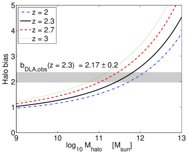
The most comprehensive DLA survey to date comes from the Baryon Oscillation Spectroscopic Survey (BOSS Dawson et al., 2013), which is part of the Sloan Digital Sky Survey III (SDSS III Eisenstein et al., 2011). The full sample, based on SDSS Data Release 9, contains over 150,000 quasar spectra over the redshift range $2.15<z<3.5$ and has discovered 6,839 DLAs, which is an order of magnitude larger than SDSS II. In particular, BOSS has for the first time estimated the bias of DLA host galaxies $(b_{\rm DLA})$ with respect to the matter distribution by cross-correlating DLA absorption with $\textrm{Ly}\alpha$ forest absorption (Font-Ribera et al., 2012). The surprisingly large value of $b_{\textrm{DLA}}=(2.17\pm 0.20)~{}\beta_{F}^{0.22}$, where $\beta_{F}\approx 1$ is the $\textrm{Ly}\alpha$ forest distortion parameter, provides an important constraint on the distribution of the host halo masses of the DLA population. Figure 1 shows the bias of dark matter haloes as a function of halo mass, for a range of redshifts including the mean redshift of the BOSS bias data, $\langle z\rangle=2.3$. The measured value of the DLA bias suggests a typical DLA halo mass of $\sim 10^{11.5}M_{\odot}$, significantly larger than is found in many simulations (e.g. Pontzen et al., 2008; Rahmati & Schaye, 2014).

Figure 1: The bias of dark matter haloes, calculated following Sheth & Tormen (2002) for a range of redshifts including the mean redshift of the BOSS bias data, $\langle z\rangle=2.3$. The observed bias and its 1 $\sigma$ error are shown as a grey shaded region, suggesting a typical DLA mass scale of $\sim 10^{11.5}M_{\odot}$.

In Barnes & Haehnelt (2009, 2010) we proposed a simple model for DLAs that simultaneously accounts for their absorption properties, and also reproduces the emission properties of a population of very faint $\textrm{Ly}\alpha$ emitters observed by Rauch et al. (2008). Here we revisit our model to see whether it can also account for the observed DLA bias. In Section 2 we describe our model for the DLA population. Section 3 compares our modelling to observations. Section 4 uses our model to place constraints on the mass-metallicity relation of DLAs, and compares this relation to the corresponding relation for luminosity-selected galaxies. In Section 5 we discuss our results and give our conclusions.

2 The DLA Model

In this section, we will summarise our model presented in Barnes & Haehnelt (2010), and discuss how we calculate the DLA bias. The cosmological parameters assumed here are $(h,~{}\Omega_{M},~{}\Omega_{b},~{}\Omega_{\Lambda},~{}\sigma_{8},~{}n,~{}Y_{p})=(0.71,~{}0.281,~{}0.0462,~{}0.719,~{}0.8,~{}0.963,~{}0.24)$. Note that the cosmological parameters have been updated from those used in Barnes & Haehnelt (2010) and that in particular the value of $\sigma_{8}$ is significantly smaller (0.8 versus 0.9).

The number density of dark matter haloes is calculated using the Press-Schechter formalism, with the elliptical-collapse ansatz of Sheth & Tormen (2002). The number of dark matter haloes per unit comoving volume at redshift $z$ with mass (baryonic + CDM) in the interval $(M_{v},M_{v}+\textrm{d}M_{v})$ is estimated as,

$$n_{M_{v}}(M_{v},z)~{}\textrm{d}M_{v}=A\left(1+\frac{1}{\nu^{\prime 2q}}\right)\sqrt{\frac{2}{\pi}}\frac{\rho_{0}}{M_{v}}\frac{\textrm{d}\nu^{\prime}}{\textrm{d}M_{v}}\exp\left(-\frac{\nu^{\prime 2}}{2}\right)~{}\textrm{d}M_{v}~{},$$ (1)

where $\sigma_{M}$ is the rms fluctuation amplitude of the cosmic density field in spheres containing mass $M_{v}$, $\rho_{0}$ is the present cosmic matter density (baryonic + CDM), $\nu^{\prime}=\sqrt{a}\nu$, $\nu=\delta_{c}/[D(z)\sigma_{M}]$. $D(z)$ is the growth factor at redshift $z$ (Carroll, Press, & Turner, 1992), $\delta_{c}=1.686$, $a=0.707$, $A\approx 0.322$ and $q=0.3$. We have used the fitting formula in Eisenstein & Hu (1999) to calculate the matter power spectrum.

We assign baryons to a given dark matter halo according to its total mass. The mass of Hi $(M_{\textrm{H{i}}})$ in a galactic halo is assumed to scale with the total virial mass $(M_{v})$ for large haloes, while being suppressed for smaller haloes due to the combined effect of photoionisation from the UV background, galactic winds and perhaps other feedback processes. This suppression is necessary to avoid overpredicting the number of DLAs with small velocity width (Haehnelt, Steinmetz, & Rauch, 1998, 2000). In our model,

$$M_{\textrm{H{i}}}=f_{\textrm{H{i}}}~{}f_{\textrm{H,c}}~{}\exp\left[-\left(\frac{v_{\textrm{v,0}}}{v_{\textrm{v}}}\right)^{\alpha_{\rm e}}\right]M_{v}$$ (2)

where $f_{\textrm{H,c}}=(1-Y_{p})\Omega_{b}/\Omega_{m}$ is the cosmic hydrogen mass fraction; $f_{\textrm{H{i}}}$ is the mass fraction of Hi in haloes, relative to cosmic; $v_{\textrm{v}}$ is the halo virial velocity, $v_{\textrm{v,0}}$ is the virial velocity below which the Hi fraction is suppressed, and $\alpha_{\rm e}$ is a parameter which determines the sharpness of the suppression.

To calculate the DLA cross-section, we need to model the distribution of neutral gas in the halo. Following the simulations of Maller & Bullock (2004, Equation (9)), we alter the NFW profile (Navarro, Frenk, & White, 1996) to give the halo gas a core at $\simeq 3r_{\textrm{s}}/4$, where $r_{\textrm{s}}$ is the scale radius of the NFW profile,

$$\rho_{\textrm{H{i}}}(r)=\frac{\rho_{0}r_{s}^{3}}{(r+\frac{3}{4}r_{\textrm{s}})(r+r_{\textrm{s}})^{2}}~{},$$ (5)

where $\rho_{0}$ normalises the profile so that the mass inside the virial radius is equal to $M_{\textrm{H{i}}}$ as specified by Equation (2); see Equation (9)-(11) of Maller & Bullock (2004). This spherically-symmetric distribution can be thought of as an effective average profile for a given halo mass.

The Hi density as a function of radius is specified by the total mass of the halo $M_{v}$ and the concentration parameter $c_{\rm v}\equiv r_{\rm v}/r_{\rm s}$ of the Hi. For the dependence of the concentration parameter on the mass, we take the mean value of the $c_{\rm v}-M_{v}$ correlation for dark matter as given by Macciò et al. (2007),

$$c_{\rm v}=c_{0}\left(\frac{M_{v}}{10^{11}M_{\odot}}\right)^{-0.109}\left(\frac{1+z}{4}\right)^{-1}~{}.$$ (6)

For dark matter, Macciò et al. (2007) found that $c_{0}\approx 3.5$, with a log-normal distribution and a scatter around this mean value of $\Delta(\ln c_{\rm v})=0.33$, in agreement of the results of Bullock et al. (2001) and Wechsler et al. (2002). As in Barnes & Haehnelt (2010), we will find later that a significantly larger $c_{0}$ is required for the baryons; we will use the column density distribution of DLAs to constrain $c_{0}$. The gas in the DLAs can be expected to self-shield against the meta-galactic ionizing UV background. The corresponding self-shielding radius in the DM haloes we are studying here is generally smaller than the virial radius. We therefore set the outer radius of the Hi to be the virial radius. Given the number density of Hi atoms $n_{\textrm{H{i}}}=\rho_{\textrm{H{i}}}/m_{H}$, we can use the relationship between impact parameter $b$ and column density on a line of sight through the system,

$$N_{\textrm{H{i}}}(b)=2\int_{0}^{\sqrt{r_{v}^{2}-b^{2}}}n_{\textrm{H{i}}}\left(r=\sqrt{b^{2}+y^{2}}\right)~{}\textrm{d}y~{},$$ (7)

to calculate the DLA cross-section of a given halo,

$$\sigma_{\textrm{DLA}}=\pi b_{\textrm{DLA}}^{2}\quad\textrm{where}\quad N_{\textrm{H{i}}}(b_{\textrm{DLA}})=N_{\textrm{DLA}}\equiv 10^{20.3}\textrm{cm}^{-2}~{}.$$ (8)

Note that in reality the incidence for DLA absorption is unlikely to have unit covering factor within a given radius; thus the DLA cross-section calculated should be considered as an effective average DLA cross-section for haloes of given mass/virial velocity. See, for example, Berry et al. (2013) for more detailed modelling of the spatial distribution and kinematics of the gas contributing to the DLA cross-section.

We can now calculate the column density distribution, defined such that the number of systems ($\textrm{d}^{2}\mathcal{N}$) intersected by a random line of sight between absorption distance $X$ and $X+\textrm{d}X$, with Hi column density between $N_{\textrm{H{i}}}$ and $N_{\textrm{H{i}}}+\textrm{d}N_{\textrm{H{i}}}$ is,

$$\textrm{d}^{2}\mathcal{N} =f(N_{\textrm{H{i}}},X)~{}\textrm{d}X~{}\textrm{d}N_{\textrm{H{i}}}$$ (10)

$$\Rightarrow\quad f(N_{\textrm{H{i}}},X) =\frac{c}{H_{0}}\int n_{M_{v}}(M_{v},X)\left|\frac{\textrm{d}\sigma}{\textrm{d}N_{\textrm{H{i}}}}(N_{\textrm{H{i}}}|M_{v},X)\right|~{}\textrm{d}M_{v}.$$ (11)

The velocity width $v_{w}$ of a DLA is defined by Prochaska & Wolfe (1997) in their pioneering survey as the velocity interval encompassing 90% of the total integrated optical depth. Given the conditional probability distribution of $v_{w}$ given $v_{\textrm{v}}$, $p(v_{\textrm{w}}|v_{\textrm{v}})~{}\textrm{d}v_{\textrm{w}}$, we can calculate the distribution of DLA velocity width along a random line of sight per unit absorption distance,

$$l(v_{\textrm{w}},X)=\frac{c}{H_{0}}\int p(v_{\textrm{w}}|v_{\textrm{v}}(M_{v}))~{}n_{M_{v}}(M_{v},X)~{}\sigma_{\textrm{DLA}}(M_{v},X)~{}\textrm{d}M_{v},~{}.$$ (12)

The distribution $p(v_{\textrm{w}}|v_{\textrm{c}})$ is chosen to have lognormal form in $x_{v}\equiv v_{w}/v_{\textrm{v}}$,

$$p(x_{v})=\frac{1}{x_{v}\sqrt{2\pi}\sigma}\exp\left({-\frac{(\ln x_{v}-\mu)^{2}}{2\sigma^{2}}}\right),$$ (13)

where we parameterize the distribution using the peak $x_{\textrm{peak}}$ and full width half maximum $x_{\textrm{FWHM}}$. In previous works, we have used $p(v_{\textrm{w}}|v_{\textrm{c}})$, drawn from the simulations of Pontzen et al. (2008). This distribution is approximately fit by a lognormal distribution with $x_{\textrm{peak}}\approx 0.61$, $x_{\textrm{FWHM}}\approx 0.45$. A lognormal distribution is also found by Neeleman et al. (2013) to fit the observed velocity width distribution. As we will see later, we need to leave $x_{\textrm{peak}}$ and $x_{\textrm{FWHM}}$ as free parameters in order to simultaneously reproduce the velocity width distribution and the DLA bias parameter $b_{\rm D}$.

Finally, we calculate the DLA bias $b_{\rm D}(z)$ in our model as,

$$b_{\rm D}(z)=\frac{\int_{0}^{\infty}b_{\rm h}(M,z)~{}n_{M_{v}}(M_{v},z)~{}\sigma_{\textrm{\rm DLA}}(M_{v},z)~{}~{}\textrm{d}M_{v}}{\int_{0}^{\infty}n_{M_{v}}(M_{v},z)~{}\sigma_{\textrm{\rm DLA}}(M_{v},z)~{}~{}\textrm{d}M_{v}}~{},$$ (16)

where $b_{\rm h}(M_{v},z)$ is the bias of dark matter haloes as a function of mass and redshift. The halo bias is calculated using the ellipsoidal collapse model of Sheth & Tormen (2002), and shown in Figure 1.

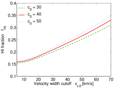
Finally, the mean redshift of observations is slightly different for the column density, velocity width and bias samples. This is taken into account in the model. The free parameters of the model are then the fraction of Hi in the halo relative to cosmic $f_{\textrm{H{i}}}$, the normalisation of the Hi concentration-mass relation $c_{0}$, the location $v_{\textrm{v,0}}$ and sharpness $\alpha_{\rm e}$ of the low-mass suppression of Hi, and the two parameters constraining the peak and width of the distribution of DLA velocity width. We will constrain these parameters using the Hi column density distribution, the DLA velocity width distribution, and the DLA bias. In particular, we will hold $\textrm{d}\mathcal{N}/\textrm{d}X=\int_{N_{\textrm{DLA}}}f(N_{\textrm{H{i}}},X)~{}\textrm{d}N_{\textrm{H{i}}}$ constant for all the models, which effectively fixes $f_{\textrm{H{i}}}$. The relationship between $f_{\textrm{H{i}}}$ and the other parameters of the model is shown in Figure 2. The fiducial values for each of these parameters, which will be justified in the next section, are as follows,

$$v_{\textrm{v,0}} =35~{}\textrm{km}~{}\textrm{s}^{-1}~{}, \alpha_{\rm e}=3,$$ (17)

$$\textrm{d}\mathcal{N}/\textrm{d}X =0.08~{}, c_{0}=40,$$ (18)

$$x_{\textrm{peak}} =0.7~{}, x_{\textrm{FWHM}}=0.8.$$ (19)

Figure 2: The fraction of HI in a halo as compared to cosmic $f_{\textrm{H{i}}}$, from Equation (2), is adjusted to hold $l_{\textrm{DLA}}\equiv\textrm{d}\mathcal{N}/\textrm{d}X$ constant. This plot shows the relationship between $f_{\textrm{H{i}}}$ and the normalisation of the Hi concentration-mass relation $c_{0}$, and the low-mass suppression of Hi in haloes $v_{\textrm{v,0}}$.

3 Comparison to Observations

We will first show how the model accounts for the column density and velocity width distribution of DLAs, and the constraints that are placed on the parameters of the model.

Figure 3: The Hi column density distribution $f(X,N)$ for changes in the parameters of the model, together with the data of Noterdaeme et al. (2012). The fiducial model has parameters $v_{v,0}=35~{}\textrm{km}~{}\textrm{s}^{-1}$, $c_{0}=40$, and $\textrm{d}\mathcal{N}/\textrm{d}X=0.08$, shown by the solid red line in each panel. The legend shows which parameter of the fiducial model has been changed. The bias is also shown, colour coded. The redshift assumed in the model is the mean redshift of the data, $\langle z\rangle=2.5$.

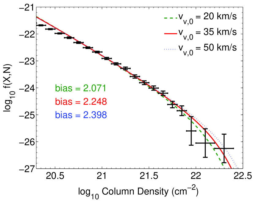
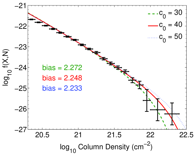
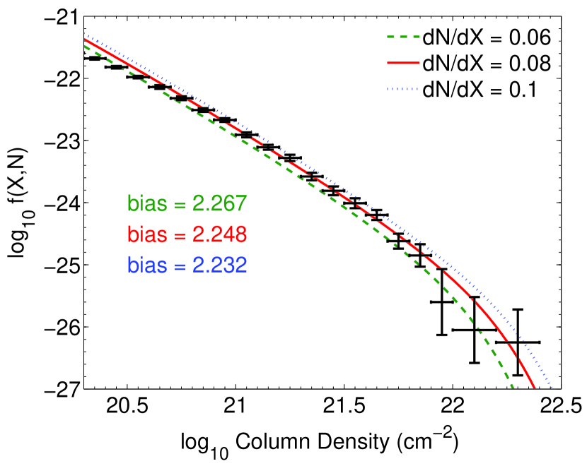
Figure 3 shows the Hi column density distribution for changes in the parameters of the model, together with the data of Noterdaeme et al. (2012). The redshift assumed in the model is the mean redshift of the data, $\langle z\rangle=2.5$. The fiducial model (solid red in each panel) is a good fit to the data. There is a slight overprediction at low $N_{\textrm{H{i}}}$, most likely due to the flattening of the observed $f(X,N)$ as we approach the LLS regime in which photoionisation effects are relevant (Rahmati et al., 2013); we have neglected such effects in our modelling. Note that our chosen value of $\textrm{d}\mathcal{N}/\textrm{d}X$ is slightly higher than observed (Prochaska & Wolfe, 2009) to take this into account.

The effect of $v_{v,0}$ on $f(X,N)$ is largely due to the dependence of $f_{\textrm{H{i}}}$ on $v_{v,0}$. As $v_{v,0}$ increases, gas is removed from low mass haloes, and thus $f_{\textrm{H{i}}}$ must increase to hold $\textrm{d}\mathcal{N}/\textrm{d}X$ constant. The top right panel shows that the high $N_{\textrm{H{i}}}$ turnover of $f(X,N)$ constrains $c_{0}$ to about 25%. Increasing the concentration of the Hi in a given halo increases the maximum $N_{\textrm{H{i}}}$ for sightlines passing through the halo. This puts higher $N_{\textrm{H{i}}}$ in smaller, more abundant haloes, boosting the high $N_{\textrm{H{i}}}$ end of the distribution function. The bottom left panel justifies the choice of $\textrm{d}\mathcal{N}/\textrm{d}X=0.08$, the other lines passing under or over almost all of the data.

Figure 4: The effect of changing modelling parameters on the DLA velocity width distribution $l(v_{w},X)$. The black crosses show the data from Wolfe, Gawiser, & Prochaska (2005). The redshift assumed in the model is the mean redshift of the data, $\langle z\rangle=3$; Pontzen et al. (2008) and Neeleman et al. (2013) note that there is very little redshift evolution. The lower right panel compares the data set of Wolfe, Gawiser, & Prochaska (2005) with Neeleman et al. (2013), and shows our best fit model for each. The best fit model to the Neeleman et al. data (green dashed line, “N13 Model”) has a conditional velocity width distribution $p(v_{\textrm{w}}|v_{\textrm{c}})$ that is narrower and peaks at a lower value than the fiducial model $x_{\textrm{peak}}=0.6$, $x_{\textrm{FWHM}}=0.6$. The difference between the two data sets is further discussed in an appendix.

.

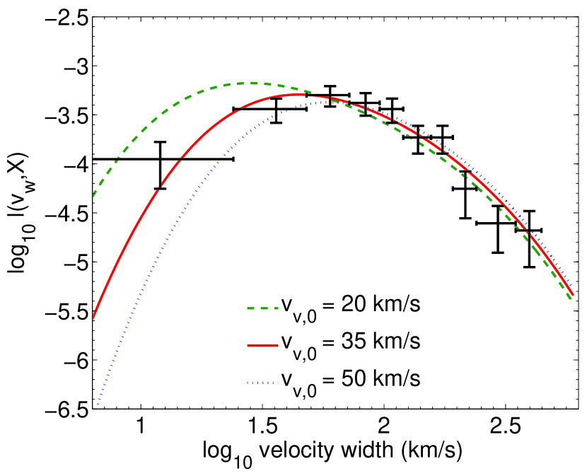
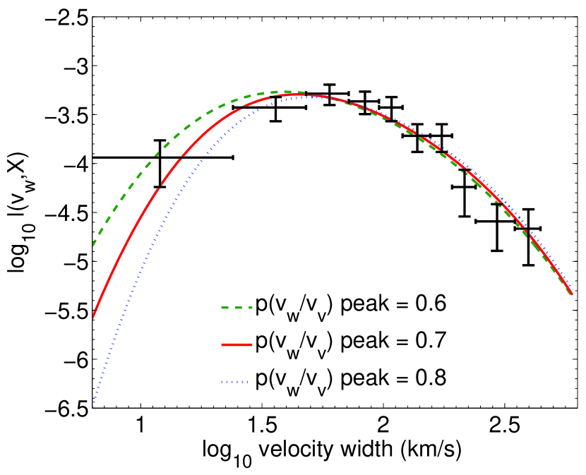
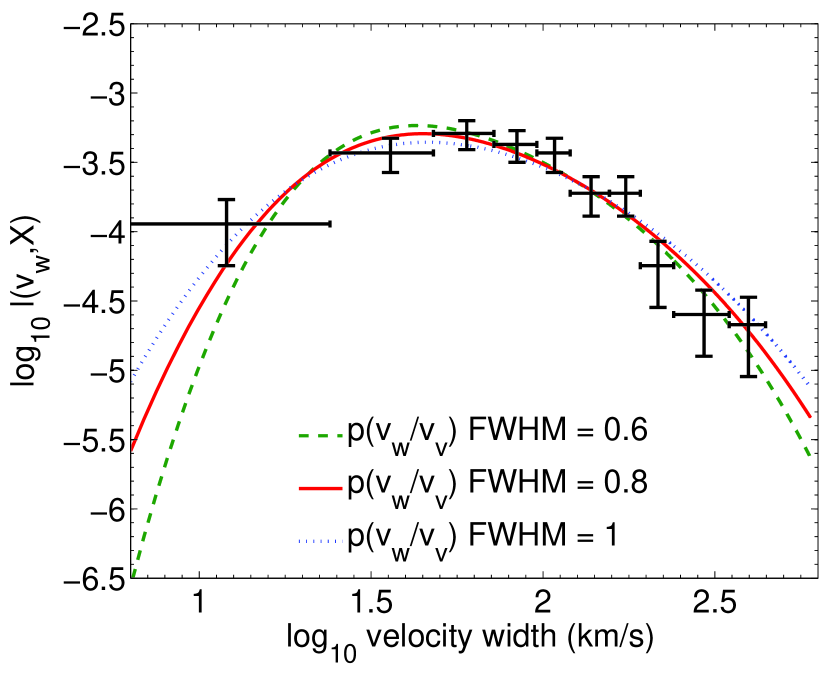
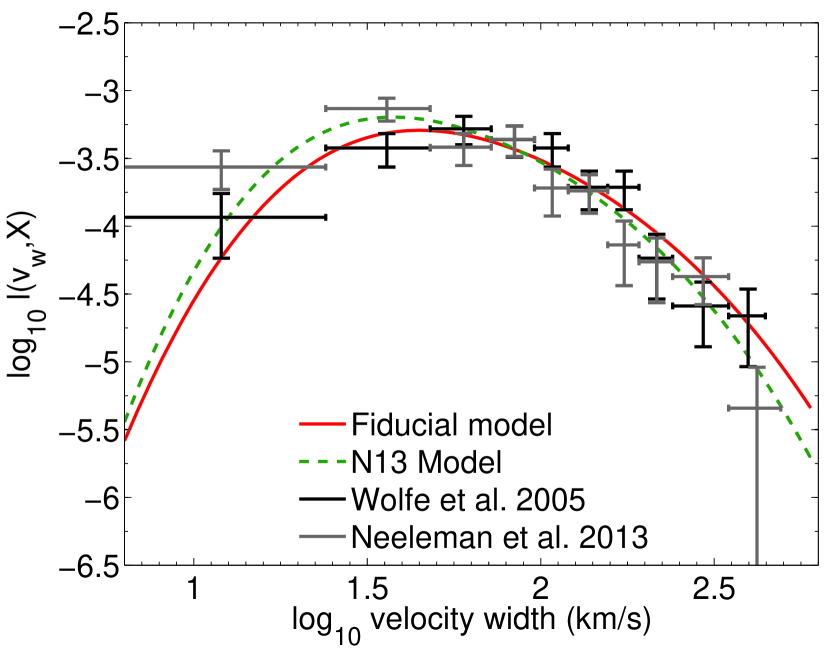
Figure 4 shows the observed velocity width distribution $l(v_{w},X)$ of low ionization absorption of DLAs from Wolfe, Gawiser, & Prochaska (2005), along with the effects of changing our model parameters. Again, our fiducial model is in red. The redshift assumed in the model is the mean redshift of the data, $\langle z\rangle=3$; Pontzen et al. (2008) and Neeleman et al. (2013) note that there is very little redshift evolution. Our fiducial model is again a reasonable fit to the data.

The top left panel shows that $v_{v,0}$ has a dramatic effect on the velocity width distribution, particularly the low end. This is expected, as the distribution $p(v_{\textrm{w}}|v_{\textrm{c}})$ in Equation (12) directly ties the velocity width to the virial velocity. Note that changing $c_{0}$ has a very small effect on $l(v_{w},X)$, and changing $\textrm{d}\mathcal{N}/\textrm{d}X$ scales each line vertically.

The top right and bottom left panels show the effect of altering the peak and FWHM of the velocity width distribution. The parameter $x_{\textrm{peak}}$ has a similar effect to $v_{v,0}$, shifting the distribution to larger/smaller velocity widths. Its value is constrained to be $\sim 0.7$. Likewise, the data constrains the width of the distribution to be $\sim 0.8$.

The bottom right panel also shows in light grey the velocity width distribution data of Neeleman et al. (2013). Note that there is a considerable difference between this data set and that of Wolfe, Gawiser, & Prochaska (2005) at the low velocity width end. We discuss this further in an appendix. The solid red line shows our best-fit model for the Wolfe et al. compilation. The dashed green line shows that the Neeleman et al. data, which has significantly more low-velocity systems, can be instead be fit by a model with $x_{\textrm{peak}}=0.6$ and $x_{\textrm{FWHM}}=0.6$. The difference between the fiducial and N13 model will not affect our conclusions.

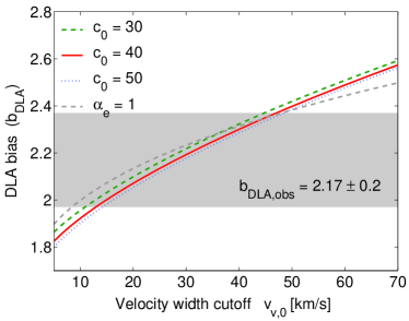
We turn now to the model’s prediction of the DLA bias. BOSS has measured the DLA bias to be $b_{\textrm{DLA}}=(2.17\pm 0.20)~{}\beta_{F}^{0.22}$. The bias is shown in Figure 3, colour coded. The redshift assumed in our model is the mean redshift of the data, $\langle z\rangle=2.3$. If we use our best fit model from previous papers, which assumed that $v_{v,0}=50$$~{}\textrm{km}~{}\textrm{s}^{-1}$, the bias is slightly overpredicted.

Our preferred value is $v_{v,0}=35$$~{}\textrm{km}~{}\textrm{s}^{-1}$; a range of parameters is shown in Figure 5. The figure shows that varying $c_{0}$ over a range consistent with the the column density and velocity width distributions does little to change our prediction of the DLA bias; changing $\textrm{d}\mathcal{N}/\textrm{d}X$ within the limits shown in Figure 3 has an even smaller effect. The grey dashed line in Figure 5 shows the effect of changing the sharpness of the Hi suppression from $\alpha_{\rm e}=3$ (so that the Hi content of galaxies is suppressed $\propto\exp(-\textrm{const}/M_{v})$) to $\alpha_{\rm e}=1$ ($\propto\exp(-\textrm{const}/v_{\textrm{v}})$). The effect on the value of $v_{v,0}$ inferred from the observed bias is small.

Figure 5: The dependence of the DLA bias $(b_{\rm DLA})$ on the parameter $v_{v,0}$, which denotes the virial velocity below which the Hi mass in haloes is exponentially suppressed. The gray shaded region shows the $\pm 1\sigma$ measurement of BOSS: $b_{\rm DLA}=(2.17\pm 0.20)~{}\beta_{F}^{0.22}$, assuming $\beta_{F}=1$. The fiducial model is in red, and the other lines show the effect of altering $c_{0}$ and $\alpha_{\rm e}$. Note that altering $\textrm{d}\mathcal{N}/\textrm{d}X$ has very little effect on the predicted bias.

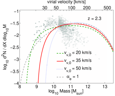
For our fiducial model, the contribution to the DLA incidence rate (Figure 6) has a broad peak from $10^{10}M_{\odot}$ to $10^{12}M_{\odot}$, a mass range that is just below the peak of the stellar mass to total halo mass obtained by dark matter halo abundance matching analyses for the stellar mass function of galaxies (Moster, Naab, & White, 2013; Behroozi, Wechsler, & Conroy, 2013).

Mechanical and thermal feedback from supernovae is generally assumed to be the mechanism by which accretion and star-formation is suppressed in low mass haloes $M_{v}<10^{11}M_{\odot}$. Note that our fiducial model requires that the peak of the velocity width distribution of DLAs $x_{\textrm{peak}}$ in a halo of given virial velocity to be slightly larger and the distribution to be wider than has been found in e.g. the simulations of DLAs by Pontzen et al. (2008).

Figure 6 shows the mass distribution of the DLA incidence rate,

$$\frac{\textrm{d}^{2}\mathcal{N}}{\textrm{d}X~{}\textrm{d}M_{v}}=\frac{c}{H_{0}}~{}n_{M_{v}}(M_{v},X)~{}\sigma_{\textrm{DLA}}(M_{v},X)~{},$$ (20)

where the fiducial model is in red, the solid lines show the effect of changing $v_{v,0}$, the dashed line shows the effect of setting $\alpha_{e}=1$, and the grey points show the DLAs of the cosmological simulation of Pontzen et al. (2008). The figure shows clearly that at the low mass end the reduction of the DLA cross-section has to extend to more massive haloes and therefore deeper potential wells than in the Pontzen et al. (2008) simulations. Our combined analysis of velocity width distribution and DLA bias therefore provides important additional clues/constraints for how stellar feedback operates in low mass haloes/shallow potential wells.

Figure 6: The contribution of different mass ranges (or, equivalently, virial velocity ranges) to the incidence rate of DLAs ($\textrm{d}^{2}N/~{}\textrm{d}X~{}\textrm{d}\log_{10}M_{v}$) at $z=2.3$. The fiducial model is in red, the solid lines show the effect of changing $v_{v,0}$, and the dashed line shows the effect of setting $\alpha_{e}=1$. Also shown in grey are the results of the cosmological simulation of Pontzen et al. (2008).

4 DLA Metallicity

We can extend our model to constrain the DLA mass-metallicity relationship. We assume a probability distribution for metallicity $[M/H]$, given halo mass $M_{v}$ and velocity width $v_{w}$, that is Gaussian with a dispersion $\sigma_{[M/H]}$ and a mean $[M/H]-v_{w},M_{v}$ relationship that we will write as,

$$[M/H]_{\textrm{mean}}=\alpha_{M}\log\left(\frac{M_{v}}{10^{11}M_{\odot}}\right)~{}+~{}\alpha_{v}\log\left(\frac{v_{w}}{\bar{x}~{}v_{\textrm{v}}(M_{v})}\right)~{}+~{}\beta_{M}~{},$$ (21)

where $\bar{x}=\textrm{e}^{\mu+\frac{1}{2}\sigma^{2}}$ is the mean of the lognormal distribution (Equation 13). This form of the relationship assumes that halo mass/virial velocity is the main controlling factor for average DLA properties, but allows for the possibility that DLAs with above average velocity width (and thus probably above average star formation rate) have above average metallicity. The mean DLA $[M/H]-M_{v}$ relation, averaging over $v_{w}$, has the form,

$$[M/H]_{\textrm{mean}}=\alpha_{M}\log\left(\frac{M_{v}}{10^{11}M_{\odot}}\right)~{}+~{}\beta_{M}~{},$$ (22)

with the same parameter values as in Equation (21).

To compare with observations, we calculate the joint probability distribution for $[M/H]$ and $v_{w}$,

$$p([M/H],v_{w})=\int p([M/H]|v_{w}M_{v})p(v_{w}|v_{\textrm{v}}(M_{v}))p(M_{v})~{}\textrm{d}M_{v}~{},$$ (23)

where the first term in the integral is the normal distribution mentioned above, the second term is the lognormal velocity width distribution of Equation (13), and the third term is the mass distribution of Equation (20), normalized to unity.

Figure 7 (left) shows the 68-95-99% contours in the $[M/H]-v_{w}$ plane, along with the data of Møller et al. (2013). The redshift of the DLAs are restricted to $2<z<4$, with a median redshift of $z=2.5$; this redshift is assumed in the model. The DLA parameters are the fiducial parameters of the model in previous sections; Equation (17). The parameters of the $[M/H]-M_{v}$ distribution are chosen by maximizing the likelihood: $(\alpha_{M},\alpha_{v},\beta_{M},\sigma_{[M/H]})=(0.47,0.08,-1.34,0.3)$. The observed distribution is slightly narrower but otherwise reasonably described by the theoretical distribution. The mean theoretical $[M/H]-v_{w}$ relation (dashed red line) passes slightly above the binned mean of the observed distribution (black points with 1-$\sigma$ SEM error bars).

Figure 7 (right) shows the observed and predicted metallicity distribution. The red line shows the same model as the red contours on the left. The black dotted and green dashed lines illustrate variations in the slope of the $[M/H]-M_{v}$ relation: $(\alpha_{M},\alpha_{v},\beta_{M})=(0.37,0.08,-1.34),~{}(0.57,0.08,-1.33)$.

Figure 7: Left: 68-95-99% contours in the $[M/H]-v_{w}$ plane, along with the data of Møller et al. (2013). The redshift of the DLAs are restricted to $2<z<4$, with a median redshift of $z=2.5$; this redshift is assumed in the model. The DLA parameters are the fiducial parameters of the model in previous sections; Equation (17). The parameters of the $[M/H]-M_{v}$ distribution are chosen by a maximizing the likelihood: $(\alpha_{M},\alpha_{v},\beta_{M},\sigma_{[M/H]})=(0.47,0.08,-1.34,0.3)$. Right: observed and predicted metallicity distribution. The red line shows the same model as the red contours on the left. The black dotted and green dashed lines illustrate variations in the slope of the $[M/H]-M_{v}$ relation: $(\alpha_{M},\alpha_{v},\beta_{M})=(0.37,0.08,-1.34),~{}(0.57,0.08,-1.33)$.

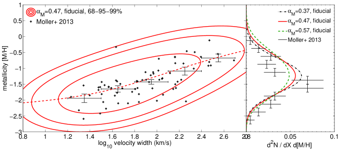
An investigation of the parameter space $(\alpha_{M},\alpha_{v},\beta_{M},\sigma_{[M/H]})$ using the Metropolis-Hastings algorithm shows that $\alpha_{M}$ and $\alpha_{v}$ are degenerate. A second, smaller peak in the probability distribution occurs at $(\alpha_{M},\alpha_{v})=(0.27,1.5)$. With no observational constraints on the halo mass of individual DLAs, such degeneracy is not surprising. The major peak at $(\alpha_{M},\alpha_{v})=(0.47,0.8)$ has a half-width $\Delta\alpha_{M}=0.1$, $\Delta\alpha_{v}=0.4$. In particular, the case $\alpha_{v}=0$ is not strongly ruled out. In summary, Figure 7 shows that DLA metallicities can be accounted for (if not predicted) in our model with a mean DLA halo mass-metallicity relationship with a slope of $0.47\pm 0.1$. At a particular halo mass, metallicity changes little with velocity width.

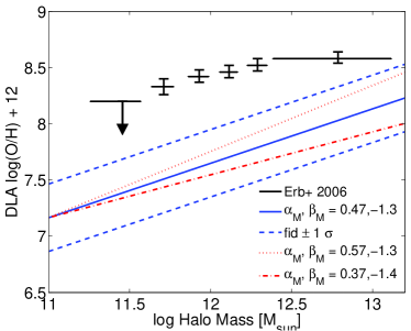
At $z\sim 2.2$, Erb et al. (2006) found that oxygen abundance $[O/H]$ increases with stellar mass. To relate this result to our mass-metallicity relationship, we need to connect DLA metallicity to [O/H], and galaxy stellar mass to halo mass. For the latter relation, we turn to the work of Behroozi, Wechsler, & Conroy (2013), who match observed galaxies to haloes to constrain the galaxy-halo relation. The derived halo mass-$[O/H]$ relation is plotted in Figure 8.

To connect DLA metallicity to $O/H$, we first connect oxygen to iron. Pettini et al. (2008) published $O/H$ and $Fe/O$ ratios for 33 DLAs with a median redshift of 2.5. The $O/H-Fe/H$ relation can be fit by the following function,

$$[Fe/H]=0.97~{}(\log(O/H)+12)-8.8~{},$$ (24)

where square brackets indicate a logarithmic abundance normalised to solar values; such values are taken from Asplund et al. (2009). The data vary by $\sigma\approx 0.17$ around this relation. Finally, Rafelski et al. (2012) note that metallicities derived from Fe include an $\alpha$-enhancement correction, $[M/H]=[Fe/H]+0.3$, giving a final $O/H$-metallicity relation of,

$$[M/H]=0.97~{}(\log(O/H)+12)-8.5$$ (25)

Combining this relation with Equation (22) gives the $O/H$-halo mass relation for our model. It is shown in Figure 8.

The black points with error bars is the galaxy stellar mass-$O/H$ relation of Erb et al. (2006), with the conversion from stellar to halo mass from Behroozi, Wechsler, & Conroy (2013), as noted above. The solid blue line shows the fiducial DLA mass-metallicity relationship of this section, $(\alpha_{M},\beta_{M})=(0.47,-1.34)$, with the dashed blue lines showing the $\pm 1\sigma_{[M/H]}$ Gaussian spread around the mean relation (Equation 22). The red dotted and dot-dashed lines show the 1-sigma variations in the mean relation, taking into account the degeneracy between $\alpha_{M}$ and $\beta_{M}$.

The metallicities measured in absorption in DLAs are significantly lower at all masses than the metallicities measured from the emission of luminosity-selected galaxies. At the same halo mass, the typical difference $\Delta\log(O/H)\sim 1$ is as expected for the metallicity difference between DLAs and LBGs (Pettini, 2006, Figure 11), consistent with two differences between the populations. First, luminosity-selected galaxies are expected to be a brighter, more evolved, and higher star-forming population. Secondly, DLA lines-of-sight are cross-section selected and so will preferentially probe the outer regions of the galaxy ($\sim 4$ kpc Pontzen et al., 2008), while LBG metallicities will tend to probe the central, star-forming region. This is consistent with the strong metallicity gradient ($-0.27\pm 0.05$ kpc^-1) observed (via gravitational lensing) in a $z=2$ galaxy (Jones et al., 2010). Note, however, that the nine galaxies (mostly at $z<1.5$ of Swinbank et al. (2012) show a shallower average metallicity gradient, in which case the large difference between the metallicities of emission- and absorption-selected galaxies may be another consequence of the velocity width-bias tension, highlighted previously.

Figure 8: Galaxy and DLA mass-$O/H$ relation. The black points with error bars is the galaxy stellar mass-$O/H$ relation of Erb et al. (2006), with the conversion from stellar to halo mass from Behroozi, Wechsler, & Conroy (2013), as noted above. The solid blue line shows the fiducial DLA mass-metallicity relationship of this section, $(\alpha_{M},\beta_{M})=(0.47,-1.34)$, with the dashed blue lines showing the $\pm 1\sigma_{[M/H]}$ Gaussian spread around the mean relation (Equation 22). The red dotted and dot-dashed lines show the 1-sigma variations in the mean slope $\alpha_{M},$, taking into account the degeneracy between $\alpha_{M}$ and $\beta_{M}$. The DLAs are significantly more metal-poor at all masses than luminosity-selected galaxies, and even more so at small masses.

5 Discussion and Conclusions

We have investigated whether our previous modelling of the physical properties of DLAs and faint $\textrm{Ly}\alpha$ emitters can account for the bias parameter estimated by BOSS for DLAs at $z\sim 2.3$. We have found that a model in which the fraction of neutral hydrogen in DM haloes drops sharply below $\sim 35$ $~{}\textrm{km}~{}\textrm{s}^{-1}$ reproduces the observed value of the DLA bias, in broad agreement with the properties of DLAs we derived from their $\textrm{Ly}\alpha$ absorption and emission.

As in Barnes & Haehnelt (2010), our model puts DLAs in more massive host haloes than, for example, the numerical simulations of Pontzen et al. (2008). This implies that stellar feedback in shallow potential wells is quite efficient at $z\ga 2.3$.

Font-Ribera et al. (2012) parameterised the absorption cross-section of DLAs as a power law $\sigma_{\textrm{DLA}}\propto M_{v}^{\alpha}$. They report that, if they fix their minimum halo mass of a DLA at $10^{9}M_{\odot}$, their observed value for the DLA bias is best fit by $\alpha=1.1\pm 0.1$. At $z=2.3$, $10^{9}M_{\odot}$ corresponds to $v_{\textrm{v}}=21~{}\textrm{km}~{}\textrm{s}^{-1}$. Such a population of DLAs in small haloes may conflict with the observed distribution of DLA velocity width, as shown in Figure 4. Berry et al. (2013) investigated the properties of DLAs in semi-analytics models of galaxy formation. They report that their favoured “BRj25” model produces a slope of $\alpha=0.91$, which is closest to the slope reported by Font-Ribera et al. (2012). However, their simulations were limited to haloes with masses $\ga 10^{9.7}$$M_{\odot}$, and the predicted bias is very sensitive to the low-mass cutoff of the DLA cross-section. If we extrapolate their $\alpha=0.91$ model to $10^{9}M_{\odot}$, the predicted bias is $\ga 2\sigma$ below the observed value. Fixing the slope, the best fit low-mass cutoff is at $10^{10.3}M_{\odot}$, which corresponds to a step-function cutoff at $v_{\textrm{v}}=56~{}\textrm{km}~{}\textrm{s}^{-1}$. The modelling of Font-Ribera et al. (2012) appears therefore to be consistent with our conclusion that some physical process needs to effectively remove or ionize gas in low mass haloes/shallow potential wells.

We use our constrained model to investigate the DLA halo mass-metallicity relation, finding $[M/H]_{\textrm{mean}}=(0.47\pm 0.1)\log\left(M_{v}/10^{11}M_{\odot}\right)-1.34$, with no significant metallicity-velocity width relation at fixed halo mass. Comparison with the galaxy stellar mass-metallicity relation finds that DLAs are typically $\Delta\log(O/H)\sim 1$ more metal-poor than luminosity-selected galaxies at all masses. We interpret this effect as evidence that DLA sightlines probe the outer regions of less-evolved galaxies.

Our modelling of DLA properties, updated to account for the large BOSS DLA bias parameter, suggests that stellar feedback in shallow potential wells is more efficient than realized in many current numerical galaxy formation models. Efficient feedback in such rather massive haloes appears also to be suggested by halo abundance matching analyses (Moster, Naab, & White, 2013; Behroozi, Wechsler, & Conroy, 2013). As many implementations of galactic winds in numerical simulations already struggle to be energetically viable, this adds to the growing consensus that either the physical mechanism behind driving galactic winds has not yet been correctly realized in numerical simulations of galaxy formation, or that other physical processes than efficient outflows are responsible for the rapidly decreasing stellar and Hi mass fraction in shallow potential wells. Further consolidation and extension of the redshift range of measurements of the bias of DLA host galaxies in combination with improved measurements of the velocity width distribution of the associated metal distribution based on larger samples should thus provide important bench marks for the modelling of stellar feedback in galaxy formation.

Appendix A The Observed DLA Velocity Width Distribution

Figure 9: A comparison of the samples of the velocity width of the associated low ionization of DLAs from Wolfe, Gawiser, & Prochaska (2005) and Neeleman et al. (2013). The left plot shows the probability of a DLA having a velocity width $v_{w}$ in a given bin. The right plot shows the cumulative probability distribution. There is a considerable difference between the two samples: for example, a Kolmogorov-Smirnov test concludes that there is a probability of $\sim 1$% that the two samples are drawn from the same underlying population.

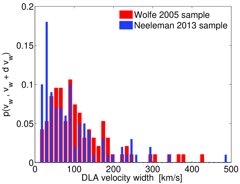
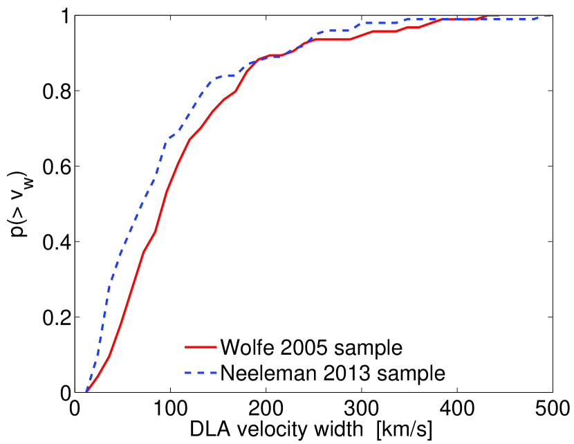
The velocity width $v_{w}$ of low-ion metal lines associated with DLAs was first investigated in detail by Prochaska & Wolfe (1997) as a probe of the kinematic state of the absorbing neutral gas inside DLAs. The distribution of $v_{w}$ has proven to be a challenge for numerical galaxy formation simulations to reproduce, as noted in the introduction. These simulations have typically attempted to model the compilation of 94 $v_{w}$ measurements of Wolfe, Gawiser, & Prochaska (2005). Recently, Neeleman et al. (2013) released a partially overlapping sample of 100 $v_{w}$ measurements, all observed with the High Resolution Echelle Spectrometer (HIRES) on the Keck I 10m telescope. A comparison of the two samples is shown in Figure 9.

The left plot shows the probability of a DLA having a velocity width $v_{w}$ in a given bin. The right plot shows the cumulative probability distribution. We note that there is a considerable difference between the two samples: for example, a Kolmogorov-Smirnov test concludes that there is a probability of $\sim 1$% that the two samples are drawn from the same underlying population.

The samples differ most at the low $v_{w}$ end, with the Neeleman et al. (2013) data set having many more systems with $v_{w}\lesssim 35~{}\textrm{km}~{}\textrm{s}^{-1}$. These are the DLAs that shed most light on the smallest haloes that are deep enough to hold their baryons against ejective feedback from supernovae and shield them from photoionisation. Given that such feedback processes are a major unknown in galaxy formation simulations, improved observations of the velocity width distribution of DLAs should thus provide a much needed stringent test of baryonic physics in low mass haloes/shallow potential wells.

References

- Asplund et al. (2009) Asplund M., Grevesse N., Sauval A. J., Scott P., 2009, ARA&A, 47, 481
- Barnes & Haehnelt (2009) Barnes L. A., Haehnelt M. G., 2009, MNRAS, 397, 511
- Barnes & Haehnelt (2010) Barnes L. A., Haehnelt M. G., 2010, MNRAS, 403, 870
- Behroozi, Wechsler, & Conroy (2013) Behroozi P. S., Wechsler R. H., Conroy C., 2013, ApJ, 770, 57
- Behroozi, Wechsler, & Conroy (2013) Behroozi P. S., Wechsler R. H., Conroy C., 2013, ApJ, 762, L31
- Berry et al. (2013) Berry M., Somerville R. S., Haas M. R., Gawiser E., Maller A., Popping G., Trager S. C., 2013, preprint (arXiv:1308.2598 )
- Bryan & Norman (1998) Bryan G. L., Norman M. L., 1998, ApJ, 495, 80
- Bullock et al. (2001) Bullock J. S., Kolatt T. S., Sigad Y., Somerville R. S., Kravtsov A. V., Klypin A. A., Primack J. R., Dekel A., 2001, MNRAS, 321, 559
- Carroll, Press, & Turner (1992) Carroll S. M., Press W. H., Turner E. L., 1992, ARA&A, 30, 499
- Christensen et al. (2007) Christensen L., Wisotzki L., Roth M. M., Sánchez S. F., Kelz A., Jahnke K., 2007, A&A, 468, 587
- Dawson et al. (2013) Dawson K. S., et al., 2013, AJ, 145, 10
- Eisenstein & Hu (1999) Eisenstein D. J., Hu W., 1999, ApJ, 511, 5
- Erb et al. (2006) Erb D. K., Shapley A. E., Pettini M., Steidel C. C., Reddy N. A., Adelberger K. L., 2006, ApJ, 644, 813
- Eisenstein et al. (2011) Eisenstein D. J., et al., 2011, AJ, 142, 72
- Font-Ribera et al. (2012) Font-Ribera A., et al., 2012, JCAP, 11, 59
- Fynbo, Møller, & Warren (1999) Fynbo J. U., Møller P., Warren S. J., 1999, MNRAS, 305, 849
- Fynbo et al. (2008) Fynbo J. P. U., Prochaska J. X., Sommer-Larsen J., Dessauges-Zavadsky M., Møller P., 2008, ApJ, 683, 321
- Haehnelt, Steinmetz, & Rauch (1998) Haehnelt M. G., Steinmetz M., Rauch M., 1998, ApJ, 495, 647
- Haehnelt, Steinmetz, & Rauch (2000) Haehnelt M. G., Steinmetz M., Rauch M., 2000, ApJ, 534, 594
- Hong et al. (2010) Hong S., Katz N., Davé R., Fardal M., Kereš D., Oppenheimer B. D., 2010, preprint (arXiv:1008.4242)
- Jones et al. (2010) Jones T., Ellis R., Jullo E., Richard J., 2010, ApJ, 725, L176
- Krogager et al. (2012) Krogager J.-K., Fynbo J. P. U., Møller P., Ledoux C., Noterdaeme P., Christensen L., Milvang-Jensen B., Sparre M., 2012, MNRAS, 424, L1
- Kulkarni et al. (2000) Kulkarni V. P., Hill J. M., Schneider G., Weymann R. J., Storrie-Lombardi L. J., Rieke M. J., Thompson R. I., Jannuzi B. T., 2000, ApJ, 536, 36
- Macciò et al. (2007) Macciò A. V., Dutton A. A., van den Bosch F. C., Moore B., Potter D., Stadel J., 2007, MNRAS, 378, 55
- Maller & Bullock (2004) Maller A. H., Bullock J. S., 2004, MNRAS, 355, 694
- Møller et al. (2013) Møller, P., Fynbo, J. P. U., Ledoux, C., & Nilsson, K. K. 2013, MNRAS, 430, 2680
- Moster, Naab, & White (2013) Moster B. P., Naab T., White S. D. M., 2013, MNRAS, 428, 3121
- Navarro, Frenk, & White (1996) Navarro J. F., Frenk C. S., White S. D. M., 1996, ApJ, 462, 563
- Neeleman et al. (2013) Neeleman M., Wolfe A. M., Prochaska J. X., Rafelski M., 2013, ApJ, 769, 54
- Noterdaeme et al. (2012) Noterdaeme P., et al., 2012, A&A, 547, L1
- Pettini (2006) Pettini M., 2006, in The Fabulous Destiny of Galaxies: Bridging Past and Present, eds. V. Le Brun, A. Mazure, S. Arnouts, & D. Burgarella. Frontier Group, Paris, p. 319
- Pettini et al. (2008) Pettini M., Zych B. J., Steidel C. C., Chaffee F. H., 2008, MNRAS, 385, 2011
- Pontzen et al. (2008) Pontzen A., et al., 2008, MNRAS, 390, 1349
- Prochaska & Wolfe (1997) Prochaska J. X., Wolfe A. M., 1997, ApJ, 487, 73
- Prochaska & Wolfe (2009) Prochaska J. X., Wolfe A. M., 2009, ApJ, 696, 1543
- Rafelski et al. (2012) Rafelski M., Wolfe A. M., Prochaska J. X., Neeleman M., Mendez A. J., 2012, ApJ, 755, 89
- Rahmati et al. (2013) Rahmati A., Pawlik A. H., Raicevic M., Schaye J., 2013, MNRAS, 430, 2427
- Rahmati & Schaye (2014) Rahmati A., Schaye J., 2014, MNRAS, 438, 529
- Rauch (1998) Rauch M., 1998, ARA&A, 36, 267
- Rauch et al. (2008) Rauch M., et al., 2008, ApJ, 681, 856
- Razoumov et al. (2008) Razoumov A. O., Norman M. L., Prochaska J. X., Sommer-Larsen J., Wolfe A. M., Yang Y.-J., 2008, ApJ, 683, 149
- Schaye (2001) Schaye J., 2001, ApJ, 559, L1
- Sheth & Tormen (2002) Sheth R. K., Tormen G., 2002, MNRAS, 329, 61
- Stringer et al. (2012) Stringer, M. J., Bower, R. G., Cole, S., Frenk, C. S., & Theuns, T. 2012, MNRAS, 423, 1596
- Swinbank et al. (2012) Swinbank A. M., Sobral D., Smail I., Geach J. E., Best P. N., McCarthy I. G., Crain R. A., Theuns T., 2012, MNRAS, 426, 935
- Tescari et al. (2009) Tescari E., Viel M., Tornatore L., Borgani S., 2009, MNRAS, 397, 411
- Wechsler et al. (2002) Wechsler R. H., Bullock J. S., Primack J. R., Kravtsov A. V., Dekel A., 2002, ApJ, 568, 52
- Wolfe, Gawiser, & Prochaska (2005) Wolfe A. M., Gawiser E., Prochaska J. X., 2005, ARA&A, 43, 861