The Quantum Spectral Curve of the ABJM Theory

Abstract

Recently, it was shown that the spectrum of anomalous dimensions and other important observables in $\mathcal{N}=4$ SYM are encoded into a simple nonlinear Riemann-Hilbert problem: the $\bf P\mu$-system or Quantum Spectral Curve. In this letter we present the $\bf P\mu$-system for the spectrum of the ABJM theory. This may be an important step towards the exact determination of the interpolating function $h(\lambda)$ characterising the integrability of the ABJM model. We also discuss a surprising symmetry between the ${\bf P}\mu$-system equations for $\mathcal{N}=4$ SYM and ABJM.

I Introduction

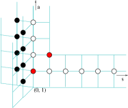
Figure 1: T-hook for the ABJM T-system

The ABJM model ABJM is a unique example of three dimensional gauge theory which may be completely solvable in the planar limit. In particular, echoing the developments in the study of $\mathcal{N}=4$ Super Yang-Mills theory in 4d, an exact description of the spectrum of conformal dimensions has been obtained by combining information from two-loop perturbation theory MinahanZarembo and on the strong coupling limit, corresponding to the classical limit of type IIA superstring theory on $AdS_{4}\times CP^{3}$ Stefanski:2008ik ; Arutyunov:2008if ; ClassicalCurve . This lead to the Asymptotic Bethe Ansatz conjectured in ABA , describing operators with large quantum numbers, and ultimately to the Thermodynamic Bethe Ansatz (TBA) equations TBA1 ; TBA2 , an infinite set of nonlinear integral equations encoding the anomalous dimensions spectrum as a function of a dressed coupling constant $h(\lambda)$. Finding the exact dependence of $h$ on the t’Hooft coupling $\lambda$ is still a missing link in the integrability approach to the ABJM theory (see Klose:2010ki for a review).

It is expected that other important observables can be studied with integrable model tools. In the case of $\mathcal{N}=4$ SYM, it was shown in MaldacenaCusp ; Drukker:2012de that a system of Boundary Thermodynamic Bethe Ansatz equations describes the (generalised) cusp anomalous dimension $\Gamma(\phi)$ characterising the logarithmic UV divergences of light-like Wilson lines forming a cusp of angle $\phi$. In some near-BPS limits, the cusp anomalous dimension can also be studied with independent localisation techniques (see for example Correa:2012at ), leading to non-perturbative exact results which nicely agree with integrability computations Gromov:2012eu ; Gromov:2013qga .

For the ABJM model, the Bremsstrahlung function $B(\lambda)$ characterising the leading small angle behaviour $\Gamma(\phi)\sim\phi^{2}B(\lambda)$ was recently computed in LastMaldacena (see also BPSWilsonLoops for related results). As already put forward in MaldacenaCusp , obtaining the same quantity with integrability methods would allow to fix the exact relation between $h$ and $\lambda$.

An important development in $\mathcal{N}=4$ SYM was the discovery of an alternative formulation of the TBA as a nonlinear matrix Riemann-Hilbert problem, known as $\bf P\mu$-system or Quantum Spectral Curve (QSC). It is a finite set of universal functional relations, believed to encode not only all states of the anomalous dimension spectrum, but also, with an appropriate change in the asymptotics, the cusp spectrum PmuAdS5 ; Gromov:2013qga . This new tool also proved to be much more efficient than the TBA for extracting exact results. In particular it lead to the 9 loop prediction for the Konishi dimension at weak coupling 9loops , $3$ loops at strong coupling QSCAtWork as well as to new results in the study of BFKL pomeron.

In this letter we present the ${\bf P\mu}$-system for the ABJM theory, and discuss a surprising link with the Quantum Spectral Curve equations for $\mathcal{N}=4$ SYM.

While here we only discuss the application of this new set of equations to the spectrum of anomalous dimensions, we believe that it will play an important r$\hat{\text{o}}$le in fixing the $h-\lambda$ relation.

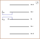
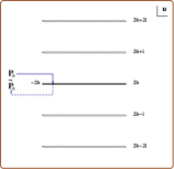
Figure 2: Analytic structure for the two types of variables in the Quantum Spectral Curve.

II Outline of the derivation

Conceptually, the $\bf P\mu$-system is equivalent to other reformulations of the TBA as a set of functional relations, such as the Y- or T-system. In particular it can be derived from the Y-system GKV supplemented by the discontinuity equations Extended ; ABJMDisc describing the monodromies of the Y functions around infinitely many branch points in the complex plane of the spectral parameter $u$. These branch points are located at rigid positions $u=\pm 2h+in/2$, $n\in\mathbb{Z}$. However these relations are very intricate, while the $\bf P\mu$-system involves only a finite number of objects, with the transparent analytic properties shown in Figure 2 PmuAdS5 : the ${\bf P}_{a}$ functions are defined on a Riemann sheet with a single cut running from $-2h$ to $+2h$, while the functions $\mu_{ab}$, although still having an infinity of branch cuts for $(-2h,+2h)+in$, $n\in\mathbb{Z}$, satisfy the simple relation

$${\tilde{\mu}}_{ab}(u)=\mu_{ab}(u+i),$$ (1)

where $\tilde{\mu}$ and ${\tilde{\bf P}}$ denote the values of the ${\bf P}\mu$ variables analytically continued around one of the branch points on the real axis. Equation (1) means that, on a different Riemann section, $\mu_{ab}$ is simply an $i$-periodic function PmuAdS5 .
To reveal this hidden structure, one can start from the analytic properties of the T functions. The T-system for the ABJM spectral problem is defined on the T-hook diagram of Figure 1 GKV , where to every node is associated a $T_{a,s}$ function. The latter satisfy the discrete Hirota equation

$$T^{[+1]}_{a,s}T^{[-1]}_{a,s}=\prod_{(a^{\prime}\sim a)_{\updownarrow}}T_{a^{\prime},s}+\prod_{(s^{\prime}\sim s)_{\leftrightarrow}}T_{a,s^{\prime}},$$ (2)

where the products are over horizontal ($\leftrightarrow$) and vertical ($\updownarrow$) neighbouring nodes and $T^{[n]}:=T(u+\frac{i}{2}n)$.

In SolvingYsystem , it was discovered a beautiful fundamental set of analyticity conditions for the T functions, and this was adapted to the ABJM case in ABJMDisc , see Appendix C of that paper. Exploiting the gauge invariance of Hirota equation, it is possible to introduce two very special gauges, denoted as ${\bf T}$ and ${\mathbb{T}}$. For $s\geq a$, the ${\mathbb{T}}_{a,s}$ functions can be parametrised as

$$\mathbb{T}_{1,s} = {\bf P}_{1}^{\left[+s\right]}{\bf P}_{2}^{\left[-s\right]}-{\bf P}_{2}^{\left[+s\right]}{\bf P}_{1}^{\left[-s\right]},\;\;\;\;\;\mathbb{T}_{0,s}=1,$$

$$\mathbb{T}_{2,s} = \mathbb{T}_{1,1}^{\left[+s\right]}\mathbb{T}_{1,1}^{\left[-s\right]},\;\;\;\;\;\mathbb{T}_{3,2}/\mathbb{T}_{2,3}=\mu_{12},$$ (3)

where ${\bf P}_{1}$, ${\bf P}_{2}$ and $\mu_{12}$ have the simple properties discussed above and will be part of the ${\bf P}\mu$-system. Furthermore, the $\bf T$ gauge can be introduced with the transformation:

$${\bf T}_{n,s} = (-1)^{n(s+1)}\mathbb{T}_{n,s}\left({\mu_{12}}^{\left[n+s-1\right]}\right)^{2-n},\hskip 28.45274pts\geq 1$$

$${\bf T}_{n,0}^{\alpha} = (-1)^{n}\mathbb{T}_{n,0}^{\alpha}\left(\sqrt{{\mu_{12}}^{\left[n-1\right]}}\right)^{2-n},$$

$${\bf T}_{n,-1}^{\alpha} = \mathbb{T}_{n,-1}^{\alpha}=1,\hskip 14.22636pt{\scriptsize\alpha=I,II},$$ (4)

and the ${\bf T}_{n,s}$ functions are required to satisfy

$${\bf T}_{n,0}^{\alpha} \in \mathcal{A}_{n+1},\hskip 14.22636pt{\scriptsize\alpha=I,II},\;\;\;n\geq 0$$

$${\bf T}_{n,1} \in \mathcal{A}_{n},\;\;\;n\geq 1,$$ (5)

where we denote with $\mathcal{A}_{n}$ the class of functions free of branch cuts in the strip $|\text{Im}(u)|<\frac{n}{2}$.

The strategy to derive the $\bf P\mu$-system, to be described in detail in AdS5Long and ABJMLong , is then the following: starting from Hirota equation and the gauge transformation (II), it is possible to compute any ${\bf T}_{n,s}$ function in terms of the only variables ${\bf P}_{1}$, ${\bf P}_{2}$, $\mu_{12}$, evaluated on different Riemann sheets. Surprisingly, when rewritten in terms of these functions, the conditions (II) show precisely how the system can be closed introducing only a finite number of fundamental variables, each with one of the two types of cut structures shown in Figure 2.

The simplest nontrivial example is provided by the condition ${\bf T}_{2,1}\in\mathcal{A}_{2}$. Computing ${\bf T}_{2,1}$ as described above, and imposing that it has no cut on the real axis, we find the constraint

$$0 = {\bf T}_{2,1}-{\tilde{\bf T}}_{2,1}$$

$$= ({\bf P}_{1}^{\left[+2\right]}{\bf P}_{2}^{\left[-2\right]}-{\bf P}_{2}^{\left[+2\right]}{\bf P}_{1}^{\left[-2\right]})\left({\tilde{\mu}}_{12}-\mu_{12}-{\bf P}_{1}{\tilde{\bf P}}_{2}+{\bf P}_{2}{\tilde{\bf P}}_{1}\right)$$

The first factor equals $\mathbb{T}_{1,2}$, which is different from zero, and this leads to a new relation:

$${\tilde{\mu}}_{12}-\mu_{12}={\bf P}_{1}{\tilde{\bf P}}_{2}-{\bf P}_{2}{\tilde{\bf P}}_{1}.$$ (7)

As will be shown in detail in ABJMLong (see AdS5Long for $\mathcal{N}=4$ SYM), the structure of the ${\bf P}\mu$-system is already revealed just by inspecting a few of the other conditions in (II).

III The ${\bf P}\mu$-system

The ${\bf P}\mu$-system for the ABJM model involves a vector of six functions ${\bf P}_{i}$, $i=1,\dots,6$ and an anti-symmetric $6\times 6$ matrix $\mu_{ab}$, with the analytic properties of Figure 2. These variables moreover satisfy the nonlinear constraints

$${\bf P}_{5}{\bf P}_{6} = 1+{\bf P}_{2}{\bf P}_{3}-{\bf P}_{1}{\bf P}_{4},$$ (8)

$$\mu\chi\mu\chi = 0.$$ (9)

The fundamental Riemann-Hilbert relations contain a $6\times 6$ symmetric matrix $\chi$ whose only nonzero entries are

$$\chi^{14}=\chi^{41}=-1,\;\;\;\chi^{23}=\chi^{32}=1,\;\;\;\chi^{56}=\chi^{65}=-1,$$

and read:

$$\tilde{{\bf P}}_{a} = {{\bf P}}_{a}-\mu_{ab}\chi^{bc}{\bf P}_{c},$$ (10)

$$\mu_{ab}-\tilde{\mu}_{ab} = -{\bf P}_{a}\tilde{\bf P}_{b}+{\bf P}_{b}\tilde{\bf P}_{a}.$$ (11)

By appropriately tuning the asymptotics, all states of the spectrum can be described by equations (8-11). Below we will discuss the asymptotics only for a specific subsector, postponing the general case to a future work ABJMLong .

Even-parity states.

For many applications it is useful to consider a reduced system of equations. As will be shown in ABJMLong , the symmetric, parity invariant sector of the spectrum is identified by the conditions ${\bf P}_{5}={\bf P}_{6}$, and $\mu_{5a}=\mu_{6a}=-\mu_{a5}=-\mu_{a6}$.

${\bf Q}\omega$-system.

Finally, we remark that, similar to the $\mathcal{N}=4$ case, there is a complementary set of conditions, named $\bf Q\omega$-system ABJMLong , which is formally the same as (8-11) with the replacements

$${\bf P}_{a}\rightarrow{\bf Q}_{a},\hskip 28.45274pt\mu_{ab}\rightarrow\omega_{ab},$$ (12)

but with all the branch cuts reversed. Namely, the functions ${\bf Q}_{a}$ have a single branch cut for $u\in(-\infty,-2\;h)\cup(+2\;h,+\infty)$, while $\omega_{ab}$ are $i$-periodic functions (with the additional interchange of some components in the nonsymmetric case) on a Riemann sheet defined with short cuts, which can be rewritten as

$$\omega_{ab}(u+i)=\omega_{\bar{a}\bar{b}}(u),$$ (13)

where $a=\bar{a}$ for $a=1,\dots,4$ and $\bar{5}=6$, $\bar{6}=5$. The physical meaning of this second system and its r$\hat{\text{o}}$le in the derivation of the Asymptotic Bethe Ansatz equations will be clarified in ABJMLong .

III.1 Identification with $\mathcal{N}=4$ SYM

An interesting formal identification is possible between (8-11) and the ${\bf P}\mu$-system previously derived for the $\mathcal{N}=4$ SYM spectral problem PmuAdS5 ; AdS5Long . This can be found by parametrising the ABJM matrix $\mu_{ab}$ in terms of 8 functions $\nu_{i}$, ${\bar{\nu}}_{i}$, $i=1,\dots,4$ as follows:

$$\mu_{ab}=\left(\begin{array}[]{cccccc}0&\nu_{1}{\bar{\nu}}_{1}&\nu_{2}{\bar{\nu}}_{2}&{\bar{\nu}}_{2}\nu_{3}-{\bar{\nu}}_{1}\nu_{4}&\nu_{1}{\bar{\nu}}_{2}&{\bar{\nu}}_{1}\nu_{2}\\ -\nu_{1}{\bar{\nu}}_{1}&0&{\bar{\nu}}_{2}\nu_{3}+\nu_{1}{\bar{\nu}}_{4}&\nu_{3}{\bar{\nu}}_{3}&\nu_{1}{\bar{\nu}}_{3}&{\bar{\nu}}_{1}\nu_{3}\\ -\nu_{2}{\bar{\nu}}_{2}&-{\bar{\nu}}_{2}\nu_{3}-\nu_{1}{\bar{\nu}}_{4}&0&\nu_{4}{\bar{\nu}}_{4}&-{\bar{\nu}}_{2}\nu_{4}&-\nu_{2}{\bar{\nu}}_{4}\\ {\bar{\nu}}_{1}\nu_{4}-{\bar{\nu}}_{2}\nu_{3}&-\nu_{3}{\bar{\nu}}_{3}&-\nu_{4}{\bar{\nu}}_{4}&0&-{\bar{\nu}}_{3}\nu_{4}&-\nu_{3}{\bar{\nu}}_{4}\\ -\nu_{1}{\bar{\nu}}_{2}&-\nu_{1}{\bar{\nu}}_{3}&{\bar{\nu}}_{2}\nu_{4}&{\bar{\nu}}_{3}\nu_{4}&0&{\bar{\nu}}_{2}\nu_{3}-\nu_{2}{\bar{\nu}}_{3}\\ -{\bar{\nu}}_{1}\nu_{2}&-{\bar{\nu}}_{1}\nu_{3}&\nu_{2}{\bar{\nu}}_{4}&\nu_{3}{\bar{\nu}}_{4}&\nu_{2}{\bar{\nu}}_{3}-{\bar{\nu}}_{2}\nu_{3}&0\end{array}\right),$$ (14)

with the additional requirement that

$$\nu_{1}{\bar{\nu}}_{4}-{\bar{\nu}}_{1}\nu_{4}=\nu_{2}{\bar{\nu}}_{3}-{\bar{\nu}}_{2}\nu_{3}.$$ (15)

By definition, $\nu_{i}$ and ${\bar{\nu}}_{i}$ have the same analytic properties as $\mu_{ab}$, namely $\widetilde{\nu}_{i}(u)=\nu_{i}(u+i)$. The parametrisation (14-15) is introduced in order to resolve the constraint $\mu\chi\mu\chi=0$. Moreover, as we discuss below, we expect that $\nu_{1}^{[+1]}$ and ${\bar{\nu}}_{1}^{[+1]}$ will play the r$\hat{\text{o}}$le of fundamental Q functions at weak coupling. Remarkably, it is possible to rewrite equations (10-11) eliminating $\mu_{ab}$ completely. In fact, one can check that all conditions (11) are satisfied provided $\nu_{i}$ and ${\bar{\nu}}_{i}$ transform in the following simple way under analytic continuation:

$$\widetilde{\nu_{i}}=U_{i}^{\;j}{\bar{\nu}}_{j},\hskip 56.9055pt\widetilde{{\bar{\nu}}_{i}}=\bar{U}_{i}^{\;j}\nu_{j},$$ (16)

where

$${U_{a}}^{b}=\left(\begin{array}[]{cccc}{\bf P}_{5}&-{\bf P}_{2}&{\bf P}_{1}&0\\ {\bf P}_{3}&-{\bf P}_{6}&0&{\bf P}_{1}\\ {\bf P}_{4}&0&-{\bf P}_{6}&{\bf P}_{2}\\ 0&{\bf P}_{4}&-{\bf P}_{3}&{\bf P}_{5}\end{array}\right),\;\;{\bar{U}_{a}}^{\;b}=\left(\begin{array}[]{cccc}{\bf P}_{6}&-{\bf P}_{2}&{\bf P}_{1}&0\\ {\bf P}_{3}&-{\bf P}_{5}&0&{\bf P}_{1}\\ {\bf P}_{4}&0&-{\bf P}_{5}&{\bf P}_{2}\\ 0&{\bf P}_{4}&-{\bf P}_{3}&{\bf P}_{6}\end{array}\right).$$ (25)

Finally, the discontinuity relations for ${\bf P}_{i}$ can be rewritten as

$${\tilde{\bf P}}_{1}-{\bf P}_{1} = \nu_{2}{\widetilde{\nu}}_{1}-\nu_{1}{\widetilde{\nu}}_{2},\;\;{\tilde{\bf P}}_{2}-{\bf P}_{2}=\nu_{3}{\widetilde{\nu}}_{1}-\nu_{1}{\widetilde{\nu}}_{3},$$

$${\tilde{\bf P}}_{3}-{\bf P}_{3} = \nu_{4}{\widetilde{\nu}}_{2}-\nu_{2}{\widetilde{\nu}}_{4},\;\;{\tilde{\bf P}}_{4}-{\bf P}_{4}=\nu_{4}{\widetilde{\nu}}_{3}-\nu_{3}{\widetilde{\nu}}_{4},$$

$${\tilde{\bf P}}_{5}-{\bf P}_{5} = \nu_{4}{\widetilde{\nu}}_{1}-\nu_{1}{\widetilde{\nu}}_{4},\;\;{\tilde{\bf P}}_{6}-{\bf P}_{6}=\nu_{3}{\widetilde{\nu}}_{2}-\nu_{2}{\widetilde{\nu}}_{3}.\hskip 28.45274pt$$ (26)

To present the identification with $\mathcal{N}=4$ SYM, for simplicity let us restrict to the symmetric sector, by taking $\nu_{i}={\bar{\nu}}_{i}$ and ${\bf P}_{5}={\bf P}_{6}$. Defining ${\bf P}_{i}^{\mathcal{N}=4}:=\nu_{i}$ for $i=1,\dots,4$ and organising the components ${\bf P}_{j}$ into a $4\times 4$ anti-symmetric matrix $\mu_{ab}^{\tiny\mathcal{N}=4}$ as shown in Table 1, one can see that, on the algebraic level, equations (16-III.1) are identical to the Quantum Spectral Curve equations for the left/right-symmetric sector of $\mathcal{N}=4$ SYM PmuAdS5 ! Even the constraints perfectly match: in fact notice that (9) translates into the constraint of PmuAdS5 :

$$({\mu_{23}}^{{\tiny\mathcal{N}=4}})^{2}=1+{\mu_{13}}^{{\tiny\mathcal{N}=4}}{\mu_{24}}^{{\tiny\mathcal{N}=4}}-{\mu_{12}}^{{\tiny\mathcal{N}=4}}{\mu_{34}}^{{\tiny\mathcal{N}=4}}.$$ (27)

Even in the non parity-invariant case, we found an identification with the ${\bf P}\mu$-system for the most general nonsymmetric sector of $\mathcal{N}=4$ SYM, described in AdS5Long . Fascinatingly, the two theories differ only in the analytic properties. As one can see from Table 1, one could transform the ABJM model into $\mathcal{N}=4$ SYM simply by exchanging the two types of cut structures presented in Figure 2, so that $i$-periodic functions $\leftrightarrow$ functions with a single cut.

$\mathcal{N}=4$ SYM	ABJM
$\mu_{ij}$,     $i,j=1,\dots,4$	$\left(\begin{array}[]{cccc}0&-{\bf P}_{1}&-{\bf P}_{2}&-{\bf P}_{0}\\ {\bf P}_{1}&0&-{\bf P}_{0}&-{\bf P}_{3}\\ {\bf P}_{2}&{\bf P}_{0}&0&-{\bf P}_{4}\\ {\bf P}_{0}&{\bf P}_{3}&{\bf P}_{4}&0\end{array}\right)$
${\bf P}_{i}$ ,     $i=1,\dots,4$	$\nu_{i}$

Table 1: The single-cut $\leftrightarrow$ periodic mapping between ABJM and $\mathcal{N}=4$ SYM (symmetric case), where we have denoted ${\bf P}_{5}={\bf P}_{6}={\bf P}_{0}$.

IV Description of the spectrum

In this Section we provide the information needed to study the subsector of the ABJM model which includes the states dual to a folded spinning string with angular momenta $L$ in $CP^{3}$ and $S$ in $AdS_{4}$. The subsector is completely characterised by the pair of integers ($L$,$S$) and by the conformal dimension $\Delta$. In the ${\bf P}\mu$-system, these quantum numbers are encoded in the asymptotics. In particular, as observed in SolvingYsystem in the $\mathcal{N}=4$ case, $\Delta$ appears in the large-$u$ behaviour of the product of Y functions $Y_{1,1}Y_{2,2}$:

$$\ln Y_{1,1}Y_{2,2}(u)=2i\frac{(\Delta-L)}{u}+\text{O}(\frac{1}{u^{2}}).$$ (28)

This quantity can be computed as

$$\ln Y_{1,1}Y_{2,2}(u)=\ln\mu_{12}(u+i)-\ln\mu_{12}(u)\sim i\partial_{u}\ln\mu_{12}(u),$$

and this implies that

$$\nu_{1}(u)=\sqrt{\mu_{12}(u)}\simeq u^{\Delta-L}.$$ (29)

The asymptotics of $\bf P$ functions is related to the $CP^{3}$ momentum $L$ as

$${\bf P}_{a}(u)\sim(A_{1}u^{-L},A_{2}u^{-L-1},A_{3}u^{+L+1},A_{4}u^{+L}),$$ (30)

with ${\bf P}_{5}={\bf P}_{6}=\sqrt{1+{\bf P}_{2}{\bf P}_{3}-{\bf P}_{1}{\bf P}_{4}}$. To complete the description of the state, we need the following relations between the coefficients $A_{i}$:

$$A_{1}A_{4} = -\frac{((\Delta-S+1)^{2}-L^{2})((\Delta+S)^{2}-L^{2})}{L^{2}(2L+1)},$$ (31)

$$A_{2}A_{3} = -\frac{((\Delta-S+1)^{2}-(L+1)^{2})((\Delta+S)^{2}-(L+1)^{2})}{(L+1)^{2}(2L+1)}.$$

Equations (31) can be derived as discussed in PmuAdS5 ; AdS5Long ; ABJMLong . It is interesting that, as remarked in QSCAtWork , the quantisation of $S$ appears naturally through the nonlinearity of the ${\bf P}\mu$-system. The identifications above involve some guesswork, but they can be checked by recovering the correct weak coupling result, as shown in the next section. In principle, equations (29-31) are the only physical input needed for the computation of $\Delta$ at any value of $h$.

IV.1 A weak coupling test

As a test of our results, let us show that they reproduce the $2$-loop Baxter equation. At leading order at weak coupling, we expect that

$$\Delta=L+S+\text{O}(h^{2}),$$ (32)

and we see from (31) that $A_{2}A_{3}=\text{O}(h^{2})$. Therefore we assume that ${\bf P}_{2}\to 0$, and we see that as a consequence the equations for $\nu_{1}$ and $\nu_{3}$ decouple:

$$\left(\begin{array}[]{c}{{\tilde{\nu}}}_{1}\\ {{\tilde{\nu}}}_{3}\end{array}\right)=\left(\begin{array}[]{c}{\nu}^{[+2]}_{1}\\ {\nu}^{[+2]}_{3}\end{array}\right)=\left(\begin{array}[]{cccc}{\bf P}_{0}&{\bf P}_{1}\\ {\bf P}_{4}&-{\bf P}_{0}\end{array}\right)\left(\begin{array}[]{c}\nu_{1}\\ \nu_{3}\end{array}\right).$$ (33)

Making the identification $\nu_{1}^{[+1]}=Q$, the system (33) implies the Baxter equation:

$$\left(\frac{{\bf P}_{0}^{[+1]}}{{\bf P}_{1}^{[+1]}}-\frac{{\bf P}_{0}^{[-1]}}{{\bf P}_{1}^{[-1]}}\right)Q=\frac{Q^{[-2]}}{{\bf P}_{1}^{[-1]}}-\frac{Q^{[+2]}}{{\bf P}_{1}^{[+1]}}.$$ (34)

Generalising the argument of PmuAdS5 , one can go further and reproduce the expected $2$-loop result MinahanZarembo :

$$\Delta = L+S+2ih^{2}\partial_{u}\log\left.\frac{Q^{[+1]}}{Q^{[-1]}}\right|_{u=0}+\text{O}(h^{4}).$$ (35)

V Conclusions

In this paper we have recast the spectral problem for the ABJM model as a finite system of coupled Riemann-Hilbert equations: the ${\bf P}\mu$-system. The similarity with the $\mathcal{N}=4$ SYM case suggests that an analogous formulation should exist also for the, still partly mysterious, integrable models related to $AdS_{3}/CFT_{2}$. Studying other examples would probably help to understand the hidden algebraic structures underlying these systems. It would be particularly interesting to investigate how the analytic properties of the ${\bf P}\mu$-system are modified under the $q$-deformation discussed in QDeformed . This may help to clarify the physical meaning of the formal map between the QSC equations for $\mathcal{N}=4$ SYM and ABJM presented in this letter.

Let us summarise some of the potential applications to ABJM. Adapting the methods of 9loops ; PmuAdS5 ; QSCAtWork , our results should allow to study the weak and strong coupling expansions, and non-perturbative near-BPS regimes such as the small-spin limit described by the slope function ABJMSlope . An interesting open problem would be to find numerical solution methods valid at generic values of the coupling. We believe that our equations can also be applied to study the spectrum of cusped Wilson lines.

Finally, one can hope that studying the ${\bf P}\mu$-system in the ABJM context would reveal some structures which are harder to see in the case of ${\cal N}=4$ SYM and help to clarify the nature and the r$\hat{\text{o}}$le of this intriguing mathematical object both in the AdS/CFT correspondence and in the general theory of integrable models. Hopefully, this can also teach us something new about non-perturbative gauge theories and AdS/CFT.

References

• (1) O. Aharony, O. Bergman, D. L. Jafferis and J. Maldacena, JHEP 0810, (2008) 091 [arXiv:0806.1218 [hep-th]].
• (2) J. A. Minahan and K. Zarembo, JHEP 0809 (2008) 040 [arXiv:0806.3951 [hep-th]].
• (3) B. Stefanski, jr, Nucl. Phys. B 808 (2009) 80 [arXiv:0806.4948 [hep-th]].
• (4) G. Arutyunov and S. Frolov, JHEP 0809 (2008) 129 [arXiv:0806.4940 [hep-th]].
• (5) N. Gromov and P. Vieira, JHEP 0902 (2009) 040 [arXiv:0807.0437 [hep-th]].
• (6) N. Gromov and P. Vieira, JHEP 0901 (2009) 016 [arXiv:0807.0777 [hep-th]].
• (7) D. Bombardelli, D. Fioravanti and R. Tateo, Nucl. Phys. B 834 (2010) 543 [arXiv:0912.4715 [hep-th]].
• (8) N. Gromov and F. Levkovich-Maslyuk, JHEP 1006 (2010) 088 [arXiv:0912.4911 [hep-th]].
• (9) T. Klose, Lett. Math. Phys.  99 (2012) 401 [arXiv:1012.3999 [hep-th]].
• (10) D. Correa, J. Maldacena and A. Sever, JHEP 1208 (2012) 134 [arXiv:1203.1913 [hep-th]].
• (11) N. Drukker, JHEP 1310 (2013) 135 [arXiv:1203.1617 [hep-th]].
• (12) D. Correa, J. Henn, J. Maldacena and A. Sever, JHEP 1206 (2012) 048 [arXiv:1202.4455 [hep-th]].
• (13) N. Gromov and A. Sever, JHEP 1211 (2012) 075 [arXiv:1207.5489 [hep-th]].
• (14) N. Gromov, F. Levkovich-Maslyuk and G. Sizov, JHEP 1310 (2013) 036 [arXiv:1305.1944 [hep-th]].
• (15) A. Lewkowycz and J. Maldacena, arXiv:1312.5682 [hep-th].
• (16) M. S. Bianchi, L. Griguolo, M. Leoni, S. Penati and D. Seminara, [arXiv:1402.4128 [hep-th]].
• (17) N. Gromov, V. Kazakov, S. Leurent and D. Volin, Phys. Rev. Lett.  112 (2014) 011602 [arXiv:1305.1939 [hep-th]].
• (18) D. Volin, to appear.
• (19) N. Gromov, F. Levkovich-Maslyuk, G. Sizov and S. Valatka, [arXiv:1402.0871 [hep-th]].
• (20) N. Gromov, V. Kazakov and P. Vieira, Phys. Rev. Lett.  103 (2009) 131601 [arXiv:0901.3753 [hep-th]].
• (21) A. Cavaglià, D. Fioravanti and R. Tateo, Nucl. Phys. B 843 (2011) 302 [arXiv:1005.3016 [hep-th]].
• (22) A. Cavaglià, D. Fioravanti and R. Tateo, Nucl. Phys. B 877 (2013) 852 [arXiv:1307.7587 [hep-th]].
• (23) N. Gromov, V. Kazakov, S. Leurent and D. Volin, JHEP 1207 (2012) 023 [arXiv:1110.0562 [hep-th]].
• (24) N. Gromov and G. Sizov, [arXiv:1403.1894 [hep-th]].
• (25) N. Gromov, V. Kazakov, S. Leurent and D. Volin, to appear.
• (26) A. Cavaglià , D. Fioravanti , N. Gromov and R. Tateo, to appear.
• (27) G. Arutyunov, M. de Leeuw and S. J. van Tongeren, JHEP 1302, 012 (2013) [arXiv:1210.8185 [hep-th]].