Delineating parton distributions and the strong coupling
Newport News, VA 23606, USA
bInstitut für Physik, Technische Universität Dortmund
D-44221 Dortmund, Germany)
Abstract
Global fits for precision determinations of parton distributions, together with the highly correlated strong coupling , are presented up to next-to-next-to-leading order (NNLO) of QCD utilizing most world data (charm and jet production data are used where theoretically possible), except TeVatron gauge boson production data and LHC data which are left for genuine predictions. This is done within the ‘dynamical’ (valencelike input at GeV2) and ‘standard’ (input at GeV2) approach. The stability and reliability of the results are ensured by including nonperturbative higher-twist terms, nuclear corrections as well as target mass corrections, and by applying various () cuts on available data. In addition, the dependence of the results is studied in detail. Predictions are given, in particular for LHC, on gauge- and Higgs-boson as well as for top-quark pair production. At NNLO the dynamical approach results in , whereas the somewhat less constrained standard fit gives .
DO-TH 14/03
JLAB-THY-14-1853
Phys. Rev. D89, 074049 (2014)
Abstract
1 Introduction
Precision determinations of parton distribution functions (PDFs), together with the strongly correlated strong coupling , are of fundamental importance for testing the expectations and predictions of the standard model (SM) of the strong, electromagnetic and weak interactions, such as the production of weak gauge bosons , of heavy quarks , of hadronic jets and, in particular, of the Higgs-boson at hadron colliders (TeVatron, LHC). A high statistical accuracy of PDFs is equally mandatory for exploring and delineating the limits of the SM, thus establishing possible signatures of approaches which go beyond the SM.
First we shall concentrate on the extraction of PDFs from presently available data within the standard approach, followed by most groups up to next-to-next-to-leading order (NNLO) of QCD [1, 2, 3, 4, 5, 6, 7, 8, 9], where the input scale is fixed at one arbitrarily chosen value GeV2. Besides the perturbative leading-twist framework (for recent reviews see, for example, [10, 11, 12]) with its strongly correlated , nonperturbative higher-twist (HT) and possible contributions are included as well, giving rise to power-like suppressed corrections proportional to . Furthermore, target-mass and nuclear deuteron corrections are also taken into account. In order to learn about the stability, and thus the reliability of the results, we perform fits to various subsets of data by applying various kinematic cuts on the available data where . In particular, the required HT contributions turn out to be sensitive to the chosen and (or ) range of the data fitted, and therefore the requirement of stable HT terms in size and shape plays a non-negligible role in all analyses. In addition we study the dependence of the results on the specific choice of the input scale (ranging from 1 to 9 GeV2 in current analyses), which in most cases has not been systematically addressed so far. In principle the results should not depend on these choices; in practice, however, a dependence develops as a consequence of what is being referred to as ‘procedural bias’ [13]. We shall start from our previous standard leading twist-2 next-to-leading order (NLO) GJR [14] and NNLO JR09 [2] analyses in order to learn about the stability and reliability of these PDFs and the values of obtained.
Next, we turn alternatively to the dynamical PDFs which are generated from input distributions at an optimally determined low input scale GeV2 ([2, 14] and references therein). This has the advantage that the input distributions naturally tend to valencelike functions, i.e., not only the valence but also the sea and gluon input densities vanish at small , due to the conventional renormalization group (RG) evolutions. Thus the behavior of parton distributions and deep inelastic scattering (DIS) structure functions at and at small is entirely predictable as a consequence of QCD dynamics (gluon and quark radiation), while in the standard approach it has to be fitted. Indeed, the very characteristic and unique steep small- predictions at were subsequently confirmed, about 20 years ago, by HERA DIS experiments ([2, 14] and references therein). These dynamical PDFs, as well as the corresponding , will be reanalyzed along very similar lines as discussed above for obtaining PDFs within the standard approach. It should be noted that the input gluon distribution for smaller than about 1 GeV2 turns out to be always valencelike. In contrast, however, present precision data do not favor a valencelike sea distribution as well: we refrain from enforcing a valencelike sea since for GeV2 the fitted value of strongly increases and decreases substantially, despite taking into account HT contributions. Therefore, in order not to deteriorate the quality of the fit and to avoid any bias towards low values, we shall fix the dynamical input scale to be GeV2 where the sea increases slightly at very small . This solution will nevertheless be referred to as dynamical, since it is the valencelike (input) gluon distribution which dominates the small- behavior of structure functions.
Section 2 is devoted to a presentation and discussion of various theoretical issues, such as the target-mass corrections to structure functions, the formulation of higher-twist contributions, nuclear corrections and the evaluation of the statistical uncertainties of PDFs. In Section 3 we present our quantitative standard and dynamical results for structure functions, PDFs and hadronic jet production. Our calculations basically refer to the so-called ‘fixed-flavor number scheme (FFNS) where heavy quarks () are not considered as massless partons within the nucleon, i.e. the number of active (light) flavors appearing in the splitting functions and corresponding Wilson coefficients will be fixed, . This scheme is fully predictive in the heavy quark sector (i.e., without any additional model assumptions) where the heavy quark flavors are produced entirely perturbatively from the initial light (u,d,s) quarks and gluons with the full heavy quark mass dependence taken into account in the production cross sections - as required experimentally, in particular, in the threshold region. In many situations, calculations within this factorization scheme become unduly complicated (for a recent discussion see, for example, [3, 15]), and in many cases even impossible due to the unknown fully massive () matrix elements at NNLO and even NLO. For this reason we shall generate, from our unique FFNS PDFs, effective PDFs in the so-called ‘variable-flavor number scheme’ (VFNS) where the heavy quarks () are considered to be massless partons within the nucleon as well. Here, the required NLO and NNLO (massless) cross sections are available in the literature for a variety of important production processes, thus allowing for predictions for gauge- and SM Higgs-boson production experiments at TeVatron and ongoing LHC measurements. It should be emphasized that, on purpose, we do not include TeVatron gauge-boson production data and LHC data in our fitting procedure which therefore allows for genuine predictions of these measurements in Section 4. Thus we can explicitly test the reliability and usefulness of the QCD improved parton model. Finally, our conclusions are summarized in Section 5.
2 Theoretical Issues
A description of the underlying QCD framework (FFNS, VFNS) used in our (JR) analyses has already been given and summarized in [2, 3] up to NNLO and will not be repeated here. However, since the last determination of our PDFs there have been some experimental and theoretical developments which deserve consideration and partly motivate the present investigations.
One of the changes in our approach is that for the SLAC [16], NMC [17] and BCDMS [18, 19] data we use now the directly measured cross sections, instead of the extracted structure functions and ratios of structure functions, since problems with such extractions have been encountered [20] (note that we have already done this for the HERA data). Additional assumptions on the spread of the beam energy would be required for reconstructing the measured cross section from the extracted E665 structure functions [21]; we have kept these data since a systematic error for the published structure functions has been provided which takes into account possible inaccuracies in the extraction (assumed value of ).
This implies that, in addition to the well-known nucleon target-mass corrections (TMCs) for [22] already included in our previous analyses, we include now TMCs for as well, which have been calculated [10, 23] in the same (operator product expansion) framework:
| (1) |
| (2) |
with the longitudinal structure function in Bjorken- space being given by .
Another issue raised by the ABM collaboration [5] is the necessity of including higher-twist contributions in the description of fixed-target data, even if moderate kinematic cuts are used to select the data included in the fits, in particular for the SLAC and NMC data [16, 17]. The kinematic cuts in our GJR and JR analyses [2, 14] were GeV2 in virtuality and GeV2 in DIS invariant mass squared, and were applied to the values extracted from different beam energies and combined. The description was good for the NMC data [17] and rather poor for SLAC data [16]. However, since the number of data points of these experiments was rather small (about 100 data points for NMC and 50 for SLAC), the values of the cuts did not affect much the results in [2] or[14]. This picture changes if data on the cross sections for individual energies are used, which amounts to hundreds of data points for each experiment. Higher twist (HT) contributions are introduced in the present investigations through the following phenomenological parametrizations:
| (3) |
where and . The function (respectively ) is a cubic spline which interpolates between a set of points, with chosen to be for and for . This choice provides enough flexibility for the additional fit parameters with respect to the data analyzed. Different choices yield similar results. Furthermore we put due to kinematic constraints, and since power-like terms appear to be not required by HERA data at small . A possible scale dependence of the and functions has been neglected.
As mentioned before, instead of ratios of structure functions we include now a wealth of deuteron cross section data [16, 17, 19, 21], so that an appropriate description of the nuclear structure is of more relevance than in our previous analyses. We use nuclear corrections provided by the CJ group [24] with the deuteron structure functions given by
| (4) |
where again and . The “smearing functions” are computed from the deuteron wave functions based on particular nucleon-nucleon potentials (we use the Paris potential [25]), and implement nuclear binding and Fermi motion effects [26, 27]. The additional additive terms represent off-shell [26] and nuclear shadowing [28] corrections (these have been considered only for the case). For the E605 [29] Drell-Yan data, as well as for the NuTeV [30] and CCFR [31] data on dimuon production in N DIS, the nuclear corrections of nDS [32] have been used. These nuclear corrections were obtained using previous sets of (3-flavor) parton distributions which are consistent with our present determinations, and therefore are especially suited for our analysis.
Yet another improvement in the present analyses is the use of the running-mass definition for DIS charm and bottom production which results in an improved stability of the perturbative series [33]. At NLO the heavy quark coefficient functions are exactly known [34, 35]. Beyond NLO the relevant coefficients are not known exactly and it has become customary to use an approximation obtained via threshold resummation and exact asymptotic () three-loop results as given in [33, 36, 37]. In order to avoid any possible ambiguities, we will rather not use DIS heavy quark data for our nominal NNLO fits. We shall come back to this point and to the relevance of such approximations in Sec. 3. In contrast to our previous analyses [2, 3, 14], the factorization scale for heavy quark production will, for consistency, be chosen to be for the relevant flavors. For all our fits we use fixed values of , and , and furthermore .
As discussed already in Sec. 1, calculations within the FFNS become unduly complicated in many situations and even impossible due to the unknown fully massive () sub-cross sections. For this reason we generate, starting from our unique flavor FFNS PDFs, efffective PDFs in the VFNS up to =5 where the ‘heavy’ quark distributions and become massless PDFs of the nucleon as well (for a recent discussion up to NNLO see, for example, [3]). We use these results for calculating jet as well as gauge- and Higgs-boson production rates.
In addition to the above improvements in the theoretical computations, a novelty in our current analysis, as compared to the published ones in [2, 3, 14], is a complete treatment of the systematic uncertainties of the data including experimental correlations. The estimator of least squares that we use to take them into account has been explicitly written down in Appendix B of [38]; we repeat it here for the convenience of the reader, and to fix the notation for further discussions. The global function is obtained as the sum of the functions of each of the data sets included in the analysis. These consist in general of data points of central value , total uncorrelated error (statistical and uncorrelated systematic errors added in quadrature), and correlated systematic errors for sources. Denoting the respective theoretical predictions by , the function for a data set is
| (5) |
where the optimal systematic shifts are not additional free parameters but rather are determined analytically as [38]
| (6) |
where denotes here the Kronecker delta. Note that in this expression the errors have been regarded as independent quantities. This is usually true for the statistical (counting) errors, while the systematic errors are often proportional to the central values, which requires a careful treatment. It is well known that naively scaling those errors as proportional to the measured central values leads to a biased estimation of the theory (towards smaller theoretical predictions), while merely taking them as proportional to the calculated central values in Eq.(5) leads to biased estimations in the opposite direction (towards larger theoretical predictions). An optimal fit can be achieved by scaling the multiplicative systematic errors as proportional to a fixed (initial) theory, and, proceeding iteratively, this theory can be self-consistently chosen to be the outcome of the estimation itself (cf. [13] for more details). Note that this method is used for the combination of inclusive HERA data as well [39].
3 Quantitative Standard and Dynamical Results
From the experimental side, besides results coming from the LHC which will not be considered for the moment, the combined (H1 + ZEUS) HERA data on neutral current and charged current DIS inclusive cross-sections [39] and charm electroproduction [40] have been published and supersede previous sets. We include as well the model-independent (based on measurements at different energies) data on and from H1 [41], and from recently analyzed BCDMS data as well as from JLab-E99118 and SLAC-E140x measurements [42]. As stated in the previous section, we have extended our theoretical description and included higher-twist contributions to the DIS structure functions, which allow us to include Jefferson Lab cross-section measurements [43] at relatively low and values, in addition to the other fixed-target DIS measurements [16, 17, 18, 19, 21, 44] already included in our previous analyses.
The dynamical determination of strange parton distributions has been investigated up to NLO in [45]. There the most precise data on dimuon production from NuTeV [30] were found in good agreement with the predictions derived from our GJR08 [14] dynamical parton distributions, which have been generated entirely radiatively starting from vanishing strange input distributions. The relevant calculation of the inclusive DIS cross section for charged current charm production is not available at NNLO; however by using the NLO expressions with NNLO distributions the would-be NNLO predictions based on vanishing strange input distributions seem to undershoot the data by more than one would expect for the size of the NNLO corrections. Thus, for lack of a better alternative, we include now the dimuon data of NuTeV [30] and CCFR [31], and appropriately extend our parametrizations to include strange-quark distributions at the input scale. Note that this also allows for the determination of a (non-perturbative) asymmetry in the strange input distributions (a perturbative asymmetry is generated by the RG evolution beyond NLO); see [45] and references therein for more details.
The nominal set of data used in our global analyses is further composed of Drell-Yan dilepton production from E605 [29], as well as proton-proton and proton-deuteron [46] and ratios of proton-deuteron to proton-proton rates from E866 [47]. Furthermore, as in our previous NLO analyses [14], we include (updated) TeVatron jet data [48, 49] in our current NLO analyses; in addition we include now DIS inclusive jet production data from HERA [50, 51]. Since the full NNLO calculations for jet cross sections are still not available, we do not include jet data in our nominal NNLO fits. (In the purely gluonic channel to dijet production the NNLO/NLO K-factor turns out to be approximately flat across the range corresponding to about a 20% increase compared to the NLO cross section [52].) However, in order to illustrate the effects of the incorrect inclusion of those data beyond NLO we carry out fits in which the data are included and the theoretical description is based on NNLO parton distributions with NLO (improved NLO in the case of TeVatron) matrix elements; these fits will be denoted by NNLO*. It should be mentioned that such an illustration might be very deceptive since the uncertainties due to the (incorrect) order of PDFs are small in comparison to the theoretical uncertainty on (the incorrect order of) matrix elements [53]. A complete list of data sets considered in our current analyses is given in Table 1. Note that the number of data points and values quoted there refer to the nominal cuts imposed on DIS data, for which we require and . No kinematic cuts were applied to Drell-Yan or jet production data, although some outliers with large errors at the limit of the kinematic coverage have been excluded from the data in [46, 48, 49].
| NDP | NLO | NNLO | NNLO* | NLO | NNLO | NNLO* | |
|---|---|---|---|---|---|---|---|
| HERA [39] | 621 | 1.44 | 1.26 | 1.38 | 1.29 | 1.19 | 1.25 |
| H1 [41] | 63 | 1.02 | 0.96 | 0.94 | 0.83 | 0.88 | 0.86 |
| H1 [41] | 63 | 1.15 | 1.14 | 1.08 | 1.71 | 1.38 | 1.25 |
| HERA [40] | 52 | 1.41 | – | 1.68 | 1.79 | – | 2.17 |
| SLAC p [16] | 504 | 1.20 | 1.16 | 1.12 | 1.14 | 1.11 | 1.10 |
| SLAC d [16] | 517 | 1.13 | 1.10 | 1.07 | 1.08 | 1.07 | 1.06 |
| BCDMS p [18] | 351 | 1.17 | 1.17 | 1.18 | 1.18 | 1.19 | 1.19 |
| BCDMS d [19] | 254 | 1.14 | 1.16 | 1.13 | 1.15 | 1.15 | 1.13 |
| NMC p, d [17] | 516 | 1.52 | 1.53 | 1.55 | 1.51 | 1.52 | 1.53 |
| NMC d/p [44] | 177 | 0.87 | 0.86 | 0.86 | 0.86 | 0.85 | 0.85 |
| E665 p, d [21] | 106 | 1.28 | 1.37 | 1.37 | 1.28 | 1.39 | 1.39 |
| JLab p [43] | 91 | 1.19 | 1.19 | 1.19 | 1.19 | 1.19 | 1.19 |
| JLab d [43] | 91 | 1.19 | 1.24 | 1.24 | 1.22 | 1.25 | 1.25 |
| BCDMS [42] | 10 | 1.32 | 1.33 | 1.19 | 1.11 | 1.10 | 1.01 |
| BCDMS [42] | 10 | 0.43 | 0.42 | 0.40 | 0.40 | 0.39 | 0.39 |
| SLAC 140x [42] | 2 | 0.39 | 0.19 | 0.28 | 0.83 | 0.44 | 0.53 |
| SLAC 140x [42] | 2 | 1.21 | 1.59 | 1.58 | 1.26 | 1.70 | 1.63 |
| dimuon [30, 31] | 180 | 0.57 | 0.56 | 0.56 | 0.56 | 0.55 | 0.55 |
| E605 [29] | 136 | 1.11 | 1.06 | 1.05 | 1.08 | 1.04 | 1.03 |
| E866 pp [46] | 138 | 1.13 | 1.10 | 1.10 | 1.13 | 1.11 | 1.11 |
| E866 pd [46] | 159 | 1.71 | 1.65 | 1.60 | 1.71 | 1.62 | 1.59 |
| E866 pd/pp [47] | 39 | 1.00 | 1.05 | 1.02 | 1.04 | 1.04 | 1.03 |
| CDF jet [48] | 64 | 2.72 | – | 1.91 | 1.97 | – | 1.61 |
| D0 jet [49] | 96 | 1.41 | – | 1.14 | 1.09 | – | 1.03 |
| ZEUS jet [50] | 30 | 0.67 | – | 0.76 | 0.61 | – | 0.66 |
| H1 jet [51] | 24 | 1.68 | – | 1.59 | 1.97 | – | 1.77 |
| total | 4296 / 4030 | 1.25 | 1.19 | 1.21 | 1.22 | 1.17 | 1.19 |
We have investigated the stability of the results under variations in these cuts. Although the effects in the parton distributions themselves are more moderate, the repercussion on the determination of the higher-twist contributions and of is quite significant. To start with, we have considered the possibility of including twist-6 contributions to the DIS structure functions, in Eq.(3). However present DIS data do not well constrain these functions: setting them free produces abnormally small values of and in conjunction with large compensating twist-4 and twist-6 contributions (this was also observed in [54]), presumably due to overfitting and blurring the scaling violations. A similar situation occurs if one uses larger cuts (like , and ) and attempts to determine simultaneously the twist-4 contributions and the parton distributions (twist-2). On the contrary, if the same larger cuts are used but only twist-2 contributions are considered, tends to larger values [5] of about 0.117 to 0.118 in our NNLO fits, and increases considerably; thus these kinds of tighter cuts should preferably be avoided. Fortunately, stable results under smaller variations in the cuts are achieved if one either uses twist-2 contributions only together with rather stringent cuts (), or twist-2 and twist-4 contributions with lower cuts similar to our nominal choice. Since the data at lower values of and provide valuable information, in particular in the large- region, we have chosen to include them and determine our parton distributions together with the twist-4 contributions; not to mention that the higher-twist contributions are of intrinsic interest themselves. Nevertheless one should keep in mind that there is an inherent uncertainty in any analysis due to data selection which ideally should be taken into consideration.
Finally it should be mentioned that we also performed a dynamical NNLO fit with a reduced cut GeV2 (together with GeV2 and twist-4 as in our nominal fit) and one with GeV2, no twist-4 and no SLAC data, which are shown in Tab. 1. The differences are rather small, even when compared with our nominal fit, as far as the final PDFs are concerned as well as : in the first case and in the second one (cf. Tab. 2 below). This indicates that both choices, as well as our nominal one, are robust.
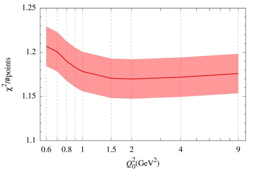
As stated in the Introduction, and in contrast to most other analyses, we do not assume a unique fixed value for the input scale , but rather pay special attention to the dependence of the results on this choice. Specifically we have considered systematic variations of this quantity ranging from 0.6 to 9 GeV2. Variations of the input scale provide information on the relative size of the so-called procedural bias, i.e. the inability of the estimation procedure to find the optimal solution, for example shortcomings of the parametrization to reproduce the optimal shape of the distributions at the different input scales, as well as of the theoretical framework and the statistical estimation procedure [13]. This is especially meaningful in the low region, in which the low- gluon and sea distributions go through a complete rearrangement of their shape, changing naturally from a valencelike structure (or even negative values) to a more conventional standard shape where they increase as decreases. Thus in addition to the systematic variations we will focus our attention on particular instances of dynamical () and standard () results, as in our previous analyses [14, 2].
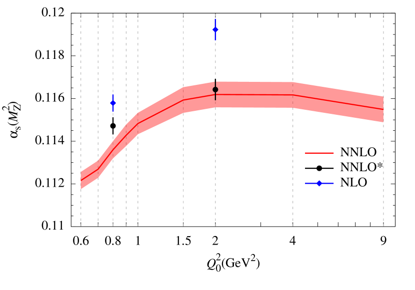
Requiring a valencelike behavior of the gluon input distribution, our fits favor a dynamical input scale of 0.8 GeV2. Smaller input scales imply increasing values of and decreasing values of according to Figs. 1 and 2, respectively, which is indicative for the increasing importance of nonperturbative contributions (higher twists). In order not to deteriorate the quality of the fit and to avoid any bias towards low values, we fix the dynamical input scale to be GeV2 where the sea increases already slightly at small . Since the valencelike input gluon distribution dominates the small- behavior of structure functions, we nevertheless refer to this solution as dynamical. Note that the distinction between dynamical and standard solutions is meaningful due to their different qualitative (physical) behavior, and is not only driven by the marginal dependence, i.e., since the value of for GeV2 in Fig. 1 is only marginally larger than for 2 GeV2, the dynamical approach can still be pursued.
On the other hand we have fixed the standard input scale to be 2 GeV2, as has become common by now, in order not to lose valuable information for fixing PDFs in particular in the large- region, as discussed above, as well as to avoid sizable backward evolutions. This specific choice of the standard input scale is of minor importance, since above about 1.5 GeV2 the final and values in Figs. 1 and 2 are practically constant. Furthermore the (incorrect) inclusion of jet (and charm) data has little influence on our nominal NNLO results for in Fig. 2 as shown by the NNLO* values at and 2 GeV2.
For each (fixed) choice of the input scale we parametrize the input parton distributions , , , , , , and . The most general parametrization of the input parton distributions that we have considered in the current analyses can be written as
| (7) |
although some of the parameters turn out to be superfluous and our nominal choice is somewhat simpler. The second term in parentheses in the gluon parametrization in principle allows for negative input gluons in the small- region. However, in all our fits the input gluon distribution remains positive, as was discussed in more detail in [13]. As a matter of fact, if one chooses a sufficiently low input scale the details of the input distribution at low do not have much influence on the predictions at higher scales, which is one of the aspects exploited in the dynamical approach to parton distributions. We also tried to keep free with different (fixed) values for and but found no significant improvement in accompanied by large correlations with other parameters; thus in our nominal parametrization we fix . Furthermore, because these parameters did not provide a considerable improvement in the description of current data and/or in order to avoid flat directions in the parameter space (which would be associated with a singular error matrix), the following parameters were treated as follows: , , , , . Note as well that the usual quark number sum rules have been imposed, so that , and in Eq.(7) are not free parameters, and similarly the momentum sum rule fixes . This amounts to a total of 25 free parameters for the parton distributions at the input scale determined together with and the 12 parameters of the higher-twist contributions (38 independent free parameters in total). Our results are shown in Tables 2 and 3.
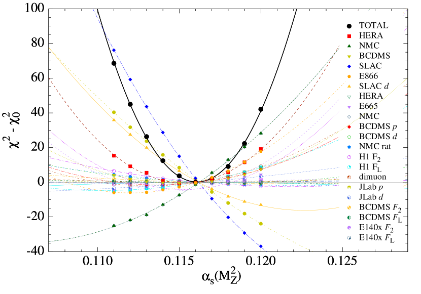
The typical dependence of on for the various sets of data used is illustrated in Fig. 3 for our standard NNLO fit. Note that these curves represent the contributions to the total of the respective data subject to the constraints of all data sets in the analysis, and thus the location of their minimum should not be strictly interpreted as the favored value by each data set (alone). Nevertheless it is interesting to see how the dependence of the total arises. We find that many data sets are rather insensitive to values; most other data favor values close to the minimum of the total , while NMC (SLAC) tend to lower (higher) values. Because of the difficulties in the interpretation of such numbers, we refrain from providing preferred values for individual data sets.
| NLO | NNLO | NLO | NNLO | |
| 0.1158 0.0004 | 0.1136 0.0004 | 0.1191 0.0005 | 0.1162 0.0006 | |
| 0.56 0.03 | 0.71 0.03 | 0.55 0.02 | 0.71 0.03 | |
| 3.51 0.03 | 3.59 0.05 | 3.61 0.03 | 3.65 0.07 | |
| 0.7 0.5 | -0.2 0.4 | 0.8 0.4 | -0.8 0.3 | |
| 6.4 0.8 | 3.8 0.5 | 4.7 0.7 | 3.4 0.3 | |
| 1.4 0.8 | 0 0.5 | -0.1 0.6 | -1.3 0.3 | |
| 0.87 0.07 | 1.30 0.06 | 0.92 0.06 | 1.10 0.05 | |
| 4.1 0.3 | 4.9 0.3 | 4.6 0.3 | 5.0 0.3 | |
| -1.9 0.4 | -3.2 0.2 | -2.8 0.3 | -3.1 0.2 | |
| 4.4 0.6 | 4.1 0.2 | 4.5 0.4 | 4.2 0.2 | |
| -2.4 0.6 | -1.5 0.3 | -2.0 0.4 | -1.7 0.4 | |
| 0.59 0.06 | 0.91 0.09 | 0.047 0.014 | 0.123 0.017 | |
| 8.3 0.4 | 12.0 0.7 | 6.1 0.2 | 7.5 0.4 | |
| 0.076 0.007 | 0.323 0.028 | 0.164 0.009 | 0.284 0.012 | |
| -0.214 0.009 | -0.070 0.010 | -0.190 0.007 | -0.150 0.005 | |
| 7.91 0.13 | 9.12 0.15 | 8.42 0.11 | 9.13 0.10 | |
| 7.8 0.9 | -2.0 0.4 | 1.9 0.3 | -1.0 0.2 | |
| 21.8 1.3 | 14.4 0.8 | 10.0 0.8 | 10.1 0.3 | |
| 57 10 | 28 6 | 37 8 | 13 3 | |
| 2.29 0.07 | 3.30 0.07 | 2.20 0.06 | 1.99 0.05 | |
| 18.6 0.9 | 19.2 0.7 | 19.2 0.5 | 19.0 0.4 | |
| 1.0 1.0 | 5.1 2.0 | 2.1 0.9 | 5.2 1.2 | |
| 0.014 0.003 | 0.081 0.014 | 0.030 0.004 | 0.058 0.008 | |
| -0.12 0.05 | 0.08 0.05 | -0.28 0.03 | -0.18 0.03 | |
| -0.007 0.008 | -0.006 0.006 | -0.006 0.005 | -0.005 0.005 | |
| 18 24 | 15 10 | 15 6 | 14 11 | |
| NLO | NNLO | NLO | NNLO | |
|---|---|---|---|---|
| -0.045 0.005 | -0.042 0.006 | -0.033 0.005 | -0.032 0.006 | |
| -0.049 0.004 | -0.036 0.004 | -0.054 0.005 | -0.037 0.005 | |
| 0.025 0.004 | 0.024 0.004 | 0.007 0.005 | 0.008 0.005 | |
| 0.041 0.003 | 0.033 0.003 | 0.031 0.003 | 0.024 0.003 | |
| -0.050 0.006 | -0.041 0.007 | -0.041 0.007 | -0.031 0.007 | |
| -0.012 0.007 | -0.002 0.007 | -0.013 0.007 | -0.003 0.007 | |
| 0.020 0.006 | 0.013 0.006 | 0.007 0.006 | 0.004 0.006 | |
| 0.016 0.004 | 0.015 0.004 | 0.014 0.004 | 0.012 0.004 | |
| 0.016 0.012 | -0.000 0.012 | 0.005 0.012 | -0.014 0.010 | |
| 0.035 0.006 | 0.027 0.006 | 0.031 0.006 | 0.024 0.006 | |
| -0.002 0.020 | -0.009 0.021 | -0.004 0.021 | -0.014 0.021 | |
| -0.005 0.011 | -0.003 0.011 | -0.001 0.011 | -0.002 0.011 | |
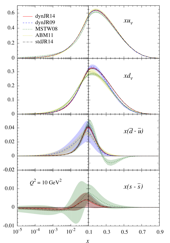
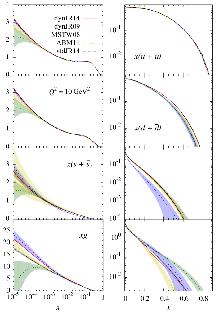
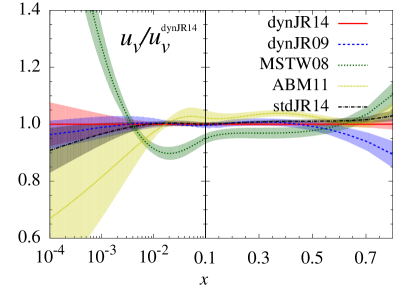
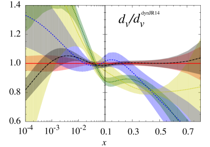
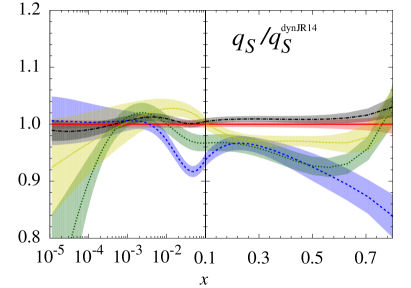
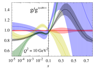
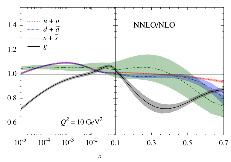
Our standard and dynamical NNLO results for the non-singlet and singlet PDFs at GeV2 are compared in Figs. 4 and 5 with our previous dynamical JR09 ones [2] as well as with the ones of MSTW08 [56] and ABM11 [5]. (The most recent global ABM12 fit [57] takes into account LHC data as well but the results turn out to be rather similar to the ones of ABM11.) Our strange sea asymmetry () in Fig. 4 is now compatible with other determinations which is in contrast to our previous JR09 result [2] where has been assumed. Similarly, our new strange sea distribution in Fig. 5 lies in the right ballpark, while the discrepancy of the much smaller JR09 result is traced back to our previously assumed input ansatz which implied a purely dynamically generated strange sea at . On the other hand, both new JR14 gluon distributions in Fig. 5 are compatible with the previous JR09 one which, in the medium- region, lie between the ones of ABM11 and MSTW08. At small , however, our gluon densities are in agreement with ABM11, taking into account that the dynamical gluon densities are steeper than the standard ones due to the longer -evolution starting at GeV2, which also implies stronger constrained (smaller errors) distributions. These features become even more transparent by plotting the respective ratios of the PDFs as done in Fig. 6. Furthermore, the differences between the NNLO and NLO distributions are depicted in Fig. 7 by the NNLO/NLO ratios of our dynamical solution. In addition, our new (dynamical) NLO PDFs are, apart from the strange sea density, similar to our previous (dynamical) NLO GJR ones [14]: at GeV2, for example, the GJR gluon is somewhat larger (by about 15% at , comparable to JR14 at , and sizably larger at large since the JR14 gluon decreases much faster as ); the density is rather similar everywhere, which holds also for except in the large- region where the GJR becomes about 30% smaller at since it decreases faster than the present one.
It should be noted that at a scale GeV2, relevant for gauge- and Higgs-boson as well as top-quark production at hadron colliders, the differences between the various sets of parton distributions in Figs. 4 – 6 become less pronounced with somewhat reduced error bands, in particular in the small-x region.
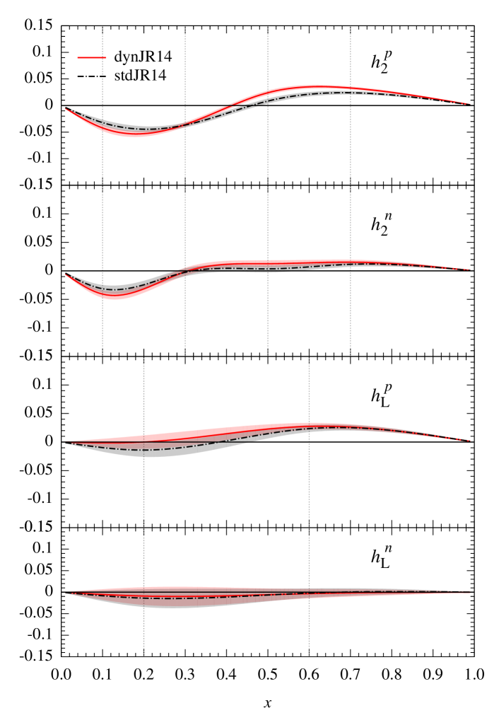
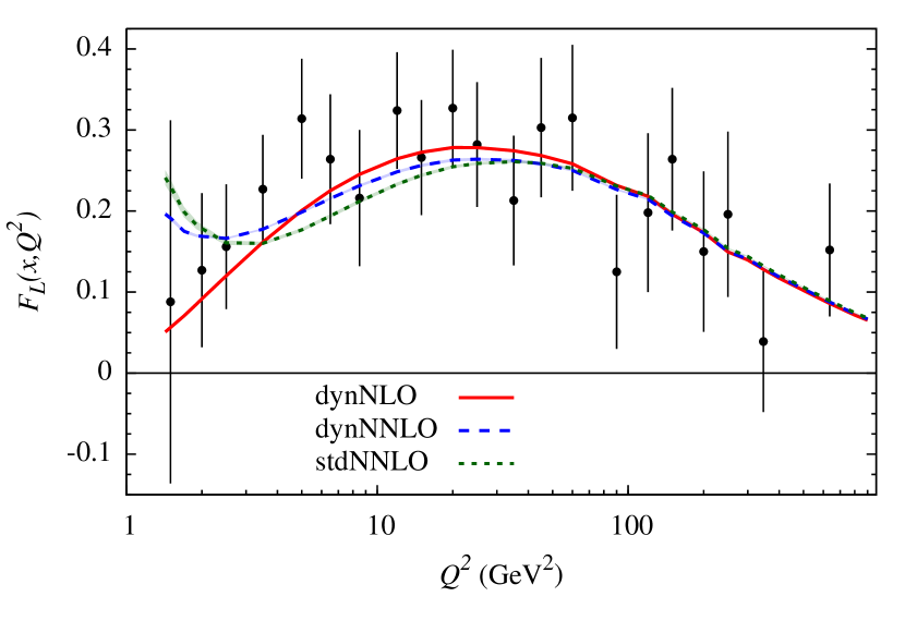
The twist-4 contributions to the structure functions in Eq. (3) are shown in Fig. 8 which are similar in shape and size as the ones obtained by ABM11 [5]. Typically, the contributions to turn negative below about 0.5 where they remain sizable and non-negligible even at moderately small values of . The higher-twist contributions to the proton longitudinal structure function are smaller at moderate values but turn significantly positive at larger , where their values are driven by JLab and SLAC data, remarkably by the separated SLAC-E140x measurements [42]. Our results for are compatible with zero within present experimental uncertainties. The inclusion of these data at large is a novelty of our global analysis and has also resulted in a sizable reduction of the experimental uncertainties on the gluon distribution at large , as can be seen in Fig. 6 (note in addition that the JR09 uncertainties [2] correspond to ). For completeness we compare in Fig. 9 our dynamical and standard predictions for with recent HERA(H1) data [41]. It should be noticed that these theoretical and experimental results cover a very large domain of which ranges from (at GeV2) to (at GeV2). Our predictions for the different proton and neutron structure functions can be obtained in [55].
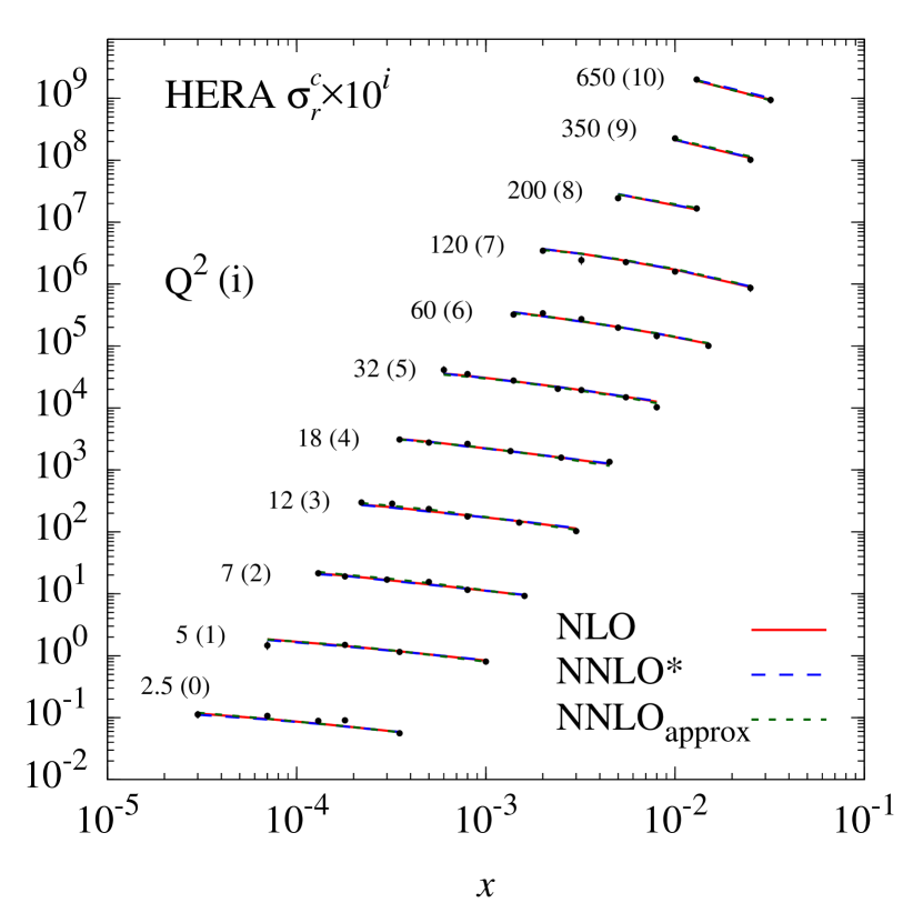
The HERA charm production data [40] are compared with our results in Fig. 10. As already discussed, we use these data only for the NLO fits due to our ignorance of the massive NNLO partonic sub-cross sections. Our dynamical NLO results are in good agreement with experiment ( per data point, according to Tab. 1). In the standard case is generally worse (cf. Tab. 1) due to the correlation between these data and the value of : the data prefer smaller values and in our case the standard fits generally tend towards larger values. The dynamical NNLO* fit shown in Fig. 10 corresponds to (see Tab. 1), but such a comparison might be deceptive since the order of the PDFs appears to be less relevant than the correct (unknown) NNLO matrix elements [53]. (If we just take our dynamical NNLO PDFs and combine them with the massive NLO Wilson coefficients (no fit), we obtain for the charm data in Fig. 10.) Finally, we compare the charm data with approximate NNLOapprox expectations as derived in [37]; such corrections to massive 3-loop Wilson coefficients are obtained by interpolating between existing soft-gluon threshold resummation results and asymptotic () coefficients [58, 59]. The interpolation uncertainty is quantified by two options [37], and , for the constant terms in the NNLO correction as a linear combination of these two options,
| (8) |
with the interpolation parameter to be fitted to the data. Our optimal NNLOapprox predictions in Fig. 10 correspond to (corresponding to ) which should be compared with [60] based on the ABM11 PDFs, and [57] based on the ABM12 PDFs. (Choosing would give instead of the optimal .) This indicates a strong dependence of on the specific PDF sets used. Anyway, the dynamical and standard NLO predictions and the various NNLO expectations in Fig. 10 are in good agreement with experiment and are practically indistinguishable. This demonstrates that the in principle unambiguous fixed-order perturbative predictions for heavy-quark production within the 3-flavor FFNS are sufficient for describing and explaining present experiments [5, 10, 14, 57, 61, 62].
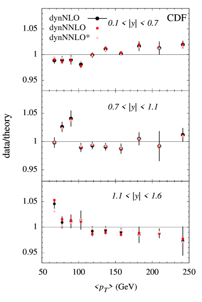
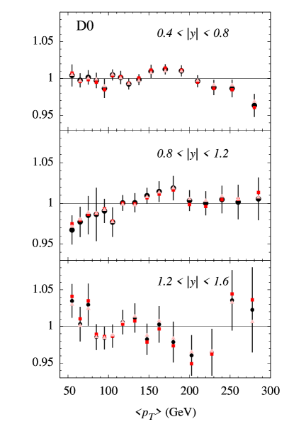
For the time being one cannot consistently use hadronic and DIS jet production measurements for NNLO analyses because the required NNLO matrix elements are not fully known yet (the calculation of these full NNLO QCD corrections is still in progress [52]). This is unfortunate since jet data are sensitive to all PDFs of the nucleon and provide the most direct constraint on the gluon distribution at large . Apart from an entirely consistent NLO analysis we nevertheless perform a NNLO fit using NLO partonic sub-cross sections (referred to as NNLO*, cf. Tab. 1) in order to check any potential impact of the jet data on our NNLO PDFs and . However, one should keep in mind that the correct order of matrix elements would be far more important than the correct order of PDFs [53]. In Fig. 11 we compare some typical representative hadronic jet-data sets with the theoretically fully consistent NLO results (the dynamical ones shown are of similar quality as the standard ones, cf. Tab. 1) as well as with the NNLO* fit and with NNLO (where jet cross sections are calculated, not fitted, as in NLO but just using our fixed NNLO PDFs). The jet data are already reasonably well described at NLO, and the differences between NLO and the theoretically inconsistent NNLO* and NNLO results are small. The same holds for the HERA jet data. This again illustrates that the incorrect order of the PDFs is not very important [53]. Furthermore, the jet data have little influence on the consistently determined NNLO value of (cf. Tab 1 and 2 where no jet data have been used) which is illustrated by the NNLO* values depicted in Fig. 2. In the standard fit the NNLO is even practically unaltered. This confirms results already obtained and emphasized in [5, 57, 63], in contrast to claims made by other PDF groups (for a comparative review, see [64], for example). A recent summary and critical discussion of current results can be found in[57].
4 Predictions for Hadron Colliders
Finally we turn to our predictions for hadron colliders. As emphasized in the Introduction, we did not include TeVatron gauge-boson production data and LHC data in our fitting procedure in order to allow for genuine predictions of these measurements. Thus one can explicitly test the reliability and usefulness of the QCD-improved parton model and of QCD in general. The general theoretical framework for hadronic weak gauge-boson () and SM Higgs-boson () production up to NNLO has been summarized in [3], for example, and will not be repeated here.
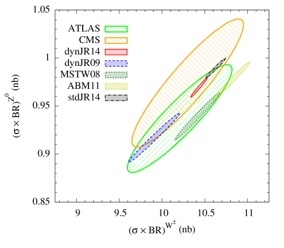
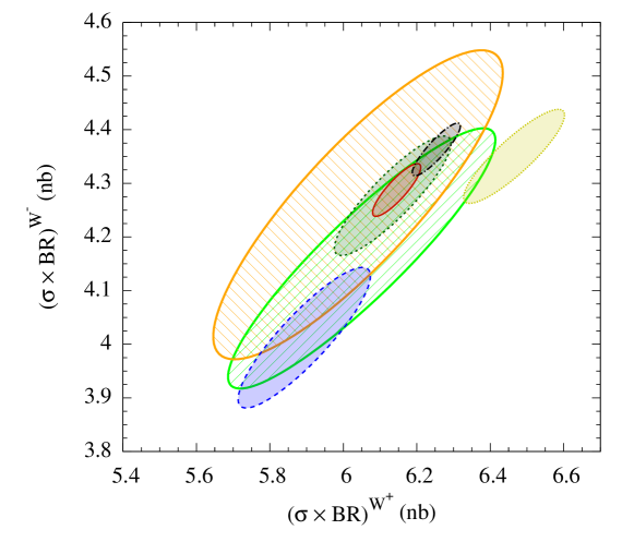
Our predictions for gauge-boson production at the TeVatron ( TeV) are given in Tab. 4 where they are compared with our previous NNLO dynamical JR09 [3] expectations as well as with the ones of ABM11 [5] and of MSTW08 [1, 56]. We confirm the slightly enhanced production rates of ABM11 which are, within , also in agreement with experiment. The predictions for LHC at , and 14 TeV are presented in Tables 5, 6, and 7, respectively. It should be noted that the and cross sections are very highly correlated, so that their ratio depends very little on specific PDFs, while the ratio of cross sections is a sensitive probe of the ratio (see, e.g., [11] for more details). To illustrate these correlations we show in Fig. 12 versus and versus total cross sections by drawing ellipses to account for the correlations between the two cross sections, both for the experimental measurements and for the theoretical predictions. The reduction of uncertainty in the cross-section ratio (cf. Tables 5 – 7) is seen as a shrinking of the corresponding ellipse, due to an improved knowlegdge of the light-quark flavor separation. It should be furthermore emphasized that our new dynamical and standard predictions in Tab. 6 are in excellent agreement with most recent CMS measurements at TeV [69].
| data | ||||||
|---|---|---|---|---|---|---|
| dynJR14 | stdJR14 | ABM11 | MSTW08 | CDF | D0 | |
| 24.07 0.14 | 24.37 0.14 | 24.2 0.3 | 23.14 0.39 | 23.16 1.12 | 21.95 1.40 | |
| (23.07 0.24) | ||||||
| 7.30 0.04 | 7.38 0.04 | 7.28 0.11 | 6.77 0.13 | 6.87 0.36 | 6.48 0.48 | |
| (6.98 0.07) | ||||||
| dynJR14 (JR09) | stdJR14 | ABM11 | MSTW08 | |
|---|---|---|---|---|
| 56.9 0.4 (54.6 1.1) | 57.9 0.4 | 59.5 0.9 | 56.8 1.0 | |
| 39.7 0.3 (37.2 0.8) | 40.4 0.3 | 40.0 0.7 | 39.6 0.7 | |
| 96.6 0.6 (91.7 1.8) | 98.4 0.7 | 99.5 1.4 | 96.4 1.6 | |
| 28.8 0.2 (27.2 0.5) | 29.4 0.2 | 29.2 0.4 | 27.9 0.5 | |
| 1.443 0.005 | 1.433 0.005 | – | – | |
| 3.351 0.040 | 3.350 0.004 | – | – | |
| 1.974 0.004 | 1.973 0.004 | – | – | |
| 1.377 0.003 | 1.377 0.003 | – | – |
| dynJR14 (JR09) | stdJR14 | ABM11 | MSTW08 | |
|---|---|---|---|---|
| 65.4 0.4 (62.6 1.4) | 66.5 0.5 | 68.3 1.0 | 65.4 1.1 | |
| 46.2 0.3 (43.3 1.0) | 47.1 0.4 | 46.7 0.8 | 46.3 0.7 | |
| 111.6 0.7 (105.9 2.3) | 113.6 0.8 | 115.0 1.7 | 111.7 1.8 | |
| 33.5 0.2 (31.6 0.6) | 34.1 0.2 | 34.0 0.5 | 33.5 +0.5 | |
| 1.413 0.005 | 1.413 0.005 | – | – | |
| 3.332 0.004 | 3.330 0.004 | – | – | |
| 1.951 0.004 | 1.950 0.004 | – | – | |
| 1.381 0.003 | 1.380 0.003 | – | – |
| dynJR14 (JR09) | stdJR14 | ABM11 | MSTW08 | |
|---|---|---|---|---|
| 114.6 0.8 (109.3 3.1) | 116.4 0.9 | 119.0 1.8 | 114.0 2.0 | |
| 85.4 0.7 (80.0 2.3) | 86.9 0.7 | 86.6 1.4 | 85.6 1.5 | |
| 200.0 1.4 (189.3 5.4) | 203.3 1.6 | 205.7 3.1 | 199.6 3.4 | |
| 61.4 0.4 (57.9 1.6) | 62.5 0.5 | 62.3 1.0 | 59.0 1.0 | |
| 1.342 0.004 | 1.340 0.004 | – | – | |
| 3.259 0.004 | 3.255 0.004 | – | – | |
| 1.867 0.003 | 1.864 0.004 | – | – | |
| 1.392 0.002 | 1.391 0.002 | – | – |
The NNLO predictions for SM Higgs-boson production at the LHC for present and future energies are given in Tab. 8 corresponding to a Higgs mass GeV [70, 71]. The theoretical uncertainty due to the scale variation dominates by far over the PDF uncertainty. We observe rather small changes with respect to our previous dynamical JR09 [3] results; the same holds true for the standard ones in Tab. 8 which are even closer to the ABM11 [5] predictions. A similar stability has been observed by ABM12 [57] where LHC data have been included in the fits. Interestingly, these predicted production rates are lower by some 10% than the ones recommended for ongoing ATLAS and CMS analyses by the HiggsXSWG [72] which read pb and pb at and 8 TeV, respectively; the second PDF uncertainties appear to be unreasonably large as compared to the PDF uncertainties in Tab. 8. For completeness we also display our predictions for Higgs-boson production at the TeVatron in Tab. 9. Our new results are, within uncertainties, comparable with the ones of other groups, although the less recent MSTW08 expectations appear to be slightly enhanced.
We close this Section with a few comments concerning the top-quark pair production at the LHC, since the calculations of the NNLO QCD corrections to hadronic production have been recently completed [73, 74, 75]. For a pole mass GeV we obtain, according to our dynamical and standard PDFs, at TeV
| (9) | |||||
| (10) |
where the central values refer to a scale choice . The scale uncertainties are due to varying between and . The second errors refer to the PDF uncertainties. For comparison, our previous dynamical JR09 [3] PDFs predict pb which is somewhat larger than in Eq. (9) due to the higher and less-constrained JR09 gluon distribution in the small- region as shown in Fig. 6; the same holds for the standard prediction in Eq. (10). These results are comparable to the ones obtained by other PDF groups [11, 57] which should be compared to the measured cross section pb [76, 77, 78].
For TeVatron measurements at TeV we predict
| (11) | |||||
| (12) |
whereas our previous dynamical JR09 [3] PDFs give pb. The combined (CDF, D0) TeVatron top-quark pair cross section is measured to be pb [78, 79].
| /TeV | dynJR14 (JR09) | stdJR14 | ABM11 | MSTW08 |
|---|---|---|---|---|
| 7 | ||||
| 8 | ||||
| 14 |
| /TeV | dynJR14 (JR09) | stdJR14 | ABM11 | MSTW08 |
|---|---|---|---|---|
| 1.8 | ||||
| 1.96 |
5 Summary and Conclusions
Utilizing recent DIS measurements and data on Drell-Yan dilepton and (partly) high- inclusive jet production, we have redone previous global fits [2, 14] for obtaining parton distributions of the nucleon of high statistical accuracy, together with the highly correlated strong coupling , up to NNLO of perturbative QCD. This has been done within the so-called dynamical GeV2) and standard ( GeV2) approaches, with being the (chosen) input scale where the RG -evolutions are started. To ensure the reliability of our results we have now included nonperturbative higher-twist (HT) terms, and nuclear corrections for the deuteron structure functions together with off-shell and nuclear shadowing corrections, as well as target-mass corrections for and . To learn about the stability of the results, we performed fits to subsets of data by applying various kinematic () cuts on the available data, since in particular the HT contributions turned out to be sensitive to such choices. A safe and stable choice turned out to be GeV2 and GeV2, which are our final nominal cuts imposed on DIS data. In addition we studied the dependence of the results on the specific choice of which in most cases has not been systematically addressed so far.
In addition to the above improvements in the theoretical computations as compared to our previous ones [2, 3, 14] is a complete treatment of the systematic uncertainties of the data including experimental correlations.
Yet another improvement is the use of the running-mass definition for DIS charm and bottom production which results in an improved stability of the perturbative series. Since heavy quark coefficient functions are exactly known only up to NLO, we have refrained from using DIS heavy-quark production data for our nominal NNLO fits. Nevertheless the NLO results are in good agreement with experiment. The same holds true when fitting charm data at NNLO using (theoretically inconsistent) NLO matrix elements (referred to as NNLO*) or approximate NNLO ones. It should, however, be kept in mind that the correct order of (massive) matrix elements appears to be far more important than the chosen order of PDFs [53]. These results demonstrate that the, in principle, unambiguous quantum-field-theoretic fixed-order perturbative predictions for heavy quark production within the fixed (three) flavor number scheme (FFNS), relying on three light flavors in the initial state, are sufficient for describing and explaining present experiments.
We face a similar situation for DIS and hadronic inclusive jet production measurements where the required sub-cross sections are not fully known yet beyond NLO, although our NLO fits agree well with present experiments (cf. Fig. 11). In order to illustrate the effects of the incorrect inclusion of these data beyond NLO, we carried out fits based on NNLO PDFs but using NLO matrix elements, again referred to as NNLO*. The differences between the NLO and the (theoretically inconsistent) NNLO* results turn out be small in the dynamical and standard approaches (cf. Fig. 11 and Tab. 1). Again, the correct order of matrix elements would be far more important [53]. Furthermore, the jet data have little influence on the consistently determined value of ; they leave essentially unaltered in NNLO standard fits with GeV2 (cf. Fig. 2).
The strong couplings obtained from our nominal dynamical NNLO (NLO) analyses are , whereas the somewhat less constrained standard fits give . Note that the uncertainties quoted here are due only to the propagation of the experimental errors of the data included in the analysis (see also [80]), while the differences between our dynamical and standard results have a systematic origin which is referred to as procedural bias. As a matter of fact it has been suggested [13] that these differences can be used to estimate these systematic uncertainties; following the procedure proposed in [13] an uncertainty of should be attributed to procedural uncertainties only. Of course, this does not exhaust the list of systematic uncertainties, choices like data selection and genuinely theoretical uncertainties like scheme and scale choices in the analysis should also be considered, and would further increase the total error. A recent summary and comparative discussion of current results can be found in [57].
It should be emphasized that, on purpose, we have not included TeVatron gauge-boson production data and LHC data in our fitting procedure, in order to allow for genuine predictions of these measurements. This allows us to explicitly test the reliability and usefulness of the QCD-improved parton model and QCD in general. Our previous dynamical (and standard) NNLO JR09 [3] predictions for the TeVatron are similar to the present new ones, confirm the somewhat enhanced production rates of ABM11 [5], and are in agreement with experiment. The same holds for our predictions for the LHC at present and future energies (, and 14 TeV) which are about 5% larger than the previous JR09 ones [3], and compare now well with the ones of ABM11 [5] and MSTW08 [1, 56], for example. The highly correlated and cross sections are in good agreement with LHC measurements at TeV, and in particular our new dynamical and standard predictions are in excellent agreement with most recent CMS measurements at TeV [69].
Our new dynamical and standard NNLO predictions for Higgs-boson production at the LHC differ rather little from our previous JR09 [3] results and are close to the ones of ABM [5, 57] (cf. Tab. 8). Interestingly, these predicted rates are lower by some 10% than the ones recommended for ongoing ATLAS and CMS analyses [72].
Our dynamical and standard PDFs and predictions, the correlation coefficients and parameter values of the eigenvector sets can be obtained on request or directly from our web page [55].
Acknowledgements
We thank S. Alekhin and J. Blümlein for several discussions and helpful comments, as well as M. Glück for a clarifying suggestion. One of us (P.J.-D.) is also indebted to W. Melnitchouk, A. Accardi and C.E. Keppel for discussions. The work of P.J.-D. was supported by DOE contract No. DE-AC05-06OR23177, under which Jefferson Science Associates, LLC operates Jefferson Lab.
References
- [1] A.D. Martin, W.J. Stirling, R.S. Thorne, and G. Watt, Eur. Phys. J. C63, 189 (2009), arXiv:0901.0002 [hep-ph].
- [2] P. Jimenez-Delgado and E. Reya, Phys. Rev. D79, 074023 (2009), arXiv:0810.4274v2 [hep-ph].
- [3] P. Jimenez-Delgado and E. Reya, Phys. Rev. D80, 114001 (2009), arXiv:0909.1711 [hep-ph].
- [4] S. Alekhin, J. Blümlein, S. Klein, and S. Moch, Phys. Rev. D81, 014032 (2010), arXiv:0908.2766 [hep-ph].
- [5] S. Alekhin, J. Blümlein, and S. Moch, Phys. Rev. D86, 054009 (2012), arXiv:1202.2281 [hep-ph].
- [6] R.D. Ball et al., NNPDF Collab., Nucl. Phys. B867, 244 (2013), arXiv:1207.1303 [hep-ph].
- [7] P. Nadolsky et al., CTEQ Collab., arXiv:1206.3321 [hep-ph].
- [8] Jun Gao et al., CTEQ Collab., Phys. Rev. D89, 033009 (2014), arXiv:1302.6246 [hep-ph].
- [9] H1 and ZEUS Collab.: V. Radescu, Proceedings of the 35th International Conference of High Energy Physics, Proceedings of Science ICHEP (2010) 168.
- [10] J. Blümlein, Prog. Part. Nucl. Phys. 69, 28 (2013), arXiv:1208.6087 [hep-ph].
- [11] S. Forte and G. Watt, Ann. Rev. Nucl. Part. Sci. 63, 291 (2013), arXiv:1301.6754 [hep-ph].
- [12] S. Alekhin, J. Blümlein, and S. Moch, Proceedings of the PIC 2012, Strbske Pleso, Slovakia, arXiv:1303.1073 [hep-ph].
- [13] P. Jimenez-Delgado, Phys. Lett. B714, 301 (2012), arXiv:1206.4262 [hep-ph].
- [14] M. Glück, P. Jimenez-Delgado, and E. Reya, Eur. Phys. J. C53, 355 (2008), arXiv:0709.0614v2 [hep-ph].
- [15] M. Glück, P. Jimenez-Delgado, E. Reya, and C. Schuck, Phys. Lett. B664, 133 (2008), arXiv:0801.3618v2 [hep-ph].
- [16] L.W. Whitlow, E.M. Riordan, S. Dasu, S. Rock, and A. Bodek, Phys. Lett. B282, 475 (1992).
- [17] M. Arneodo et al., New Muon Collab., Nucl. Phys. B483, 3 (1997), hep-ph/9610231.
- [18] A.C. Benvenuti et al., BCDMS Collab., Phys. Lett. B223, 485 (1989).
- [19] A.C. Benvenuti et al., BCDMS Collab., Phys. Lett. B237, 592 (1990).
- [20] S. Alekhin, J. Blümlein, and S. Moch, Eur. Phys. J. C71, 1723 (2011), arXiv:1101.5261 [hep-ph].
- [21] M.R. Adams et al., E665 Collab., Phys. Rev. D54, 3006 (1996).
- [22] H. Georgi and H.D. Politzer, Phys. Rev. D14, 1829 (1976).
- [23] F.M. Steffens, M.D. Brown, W. Melnitchouk, and S. Sanches, Phys. Rev. D86, 065208 (2012), arXiv:1210.4398 [hep-ph].
- [24] A. Accardi, W. Melnitchouk, J.F. Owens, M.E. Christy, C.E. Keppel, L. Zhu, and J.G. Morfin, Phys. Rev. D84, 014008 (2011), arXiv:1102.3686 [hep-ph].
- [25] M. Lacombe, B. Loiseau, J.M. Richard, R. Vinh Mau, J. Cote, P. Pires and R. De Tourreil, Phys. Rev. D21, 861 (1980).
- [26] S.A. Kulagin and R. Petti, Nucl. Phys. A765, 126 (2006), hep-ph/0412425.
- [27] Y. Kahn, W. Melnitchouk and S.A. Kulagin, Phys. Rev. C79, 035205 (2009), arXiv:0809.4308 [nucl-th].
- [28] W. Melnitchouk and A.W. Thomas, Phys. Rev. D47, 3783 (1993), nucl-th/9301016.
- [29] G. Moreno, C.N. Brown, W.E. Cooper, D. Finley, Y.B. Hsiung, A.M. Jonckheere, H. Jostlein and D.M. Kaplan et al., Phys. Rev. D43, 2815 (1991).
- [30] D. Mason et al., NuTeV Collab., Phys. Rev. Lett. 99, 192001 (2007).
- [31] M. Goncharov et al., NuTeV Collab., Phys. Rev. D64, 112006 (2001), hep-ex/0102049.
- [32] D. de Florian and R. Sassot, Phys. Rev. D69, 074028 (2004), hep-ph/0311227.
- [33] S. Alekhin and S. Moch, Phys. Lett. B699, 345 (2011), arXiv:1011.5790 [hep-ph].
- [34] E. Laenen, S. Riemersma, J. Smith, and W. van Neerven, Nucl. Phys. B392, 162 (1993).
- [35] T. Gottschalk, Phys. Rev. D23, 56 (1981); M. Glück, S. Kretzer, and E. Reya, Phys. Lett. B380, 171 (1996), hep-ph/9603304.
- [36] E. Laenen and S. Moch, Phys. Rev. D59, 034027 (1999), hep-ph/9809550.
- [37] H. Kawamura, N.A. Lo Presti, S. Moch, and A. Vogt, Nucl. Phys. B864, 399 (2012), arXiv:1205.5727 [hep-ph].
- [38] D. Stump, J. Pumplin, R. Brock, D. Casey, J. Huston, J. Kalk, H.L. Lai, and W.K. Tung, Phys. Rev. D65, 014012 (2001), hep-ph/0101051.
- [39] F.D. Aaron et al., H1 and ZEUS Collab., JHEP 01 (2010) 109, arXiv:0911.0884 [hep-ex].
- [40] H. Abramowicz et al., H1 and ZEUS Collab., Eur. Phys. J. C73, 2311 (2013), arXiv:1211.1182 [hep-ex].
- [41] F.D. Aaron et al., H1 Collab., Eur. Phys. J. C71, 1579 (2011), arXiv:1012.4355 [hep-ex]; V. Andreev et al., H1 Collab., Eur. Phys. J. C (to be published), arXiv:1312.4821 [hep-ex].
- [42] P. Monaghan et al., Phys. Rev. Lett. 110, 152002 (2013), arXiv:1209.4542 [nucl-ex].
- [43] S.P. Malace et al., Jefferson Lab E00-115 Collab., Phys. Rev. C80, 035207 (2009), arXiv:0905.2374 [nucl-ex].
- [44] M. Arneodo et al., NMC, Nucl. Phys. B487, 3 (1997), hep-ex/9611022.
- [45] P. Jimenez-Delgado, Phys. Lett. B689 (2010) 177, arXiv:1002.2104 [hep-ph].
- [46] J. Webb, FERMILAB-THESIS-2002-56,hep-ex/0301031; P.E. Reimer, private communication.
- [47] R.S. Towell et al., FNAL E866/NuSea Collab., Phys. Rev. D64, 052002 (2001), hep-ex/0103030.
- [48] T. Aaltonen et al., CDF Collab., Phys. Rev. D78, 052006 (2008), arXiv:0807.2204 [hep-ex]; Phys. Rev. D 79, 119902(E) (2009).
- [49] V.M. Abazov et al., D0 Collab., Phys. Rev. Lett. 101, 062001 (2008), arXiv:0802.2400 [hep-ex].
- [50] S. Chekanov et al., ZEUS Collab., Nucl. Phys. B765, 1 (2007), hep-ex/0608048.
- [51] A. Aktas et al., H1 Collab., Phys. Lett. B653, 134 (2007), arXiv:0706.3722 [hep-ex].
- [52] A. Gehrmann - De Ridder, T. Gehrmann, E.W.N. Glover, and J. Pires, Phys. Rev. Lett. 110, 162003 (2013), arXiv:1301.7310 [hep-ph]; J. Currie et al., JHEP 01 (2014) 110, arXiv:1310.3993 [hep-ph].
- [53] S. Forte, A. Isgrò, and G. Vita, Phys. Lett. B731, 146 (2014), arXiv:1312.6688 [hep-ph], and references therein.
- [54] S. Alekhin, S.A. Kulagin and R. Petti, Proceedings of the 15th International Workshop on Deep-Inelastic Scattering and Related Subjects (DIS2007), Munich, Germany, 16-20 April, 2007, edited by G. Grindhammer and K. Sachs, Vol.1.
- [55] http://users.hepforge.org/pjimenezdelgado
- [56] A.D. Martin, W.J. Stirling, R.S. Thorne, and G. Watt, Eur. Phys. J. C70, 51 (2010), arXiv:1007.2624 [hep-ph].
- [57] S. Alekhin, J. Blümlein, and S. Moch, Phys. Rev. D89, 054028 (2014), arXiv:1310.3059 [hep-ph].
- [58] I. Bierenbaum, J. Blümlein, and S. Klein, Nucl. Phys. B820, 417 (2009), arXiv:0904.3563 [hep-ph].
- [59] J. Ablinger et al., Nucl. Phys. B844, 26 (2011), arXiv:1008.3347 [hep-ph].
- [60] S. Alekhin et al., Phys. Lett. B720, 172 (2013), arXiv:1212.2355 [hep-ph].
- [61] S. Alekhin and S. Moch, Phys. Lett. B699, 345 (2011), arXiv:1011.5790 [hep-ph].
- [62] P. Jimenez-Delgado, W. Melnitchouk, and J.F. Owens, J. Phys. G. 40, 093102 (2013), arXiv:1306.6515v3 [hep-ph].
- [63] S. Alekhin, J. Blümlein, and S. Moch (2011), arXiv:1105.5349 [hep-ph].
- [64] R.S. Thorne and G. Watt, JHEP 08 (2011) 100, arXiv:1106.5789 [hep-ph]
- [65] A. Abulencia et al., CDF Collab., J. Phys. G 34, 2457 (2007), hep-ex/0508029, and references therein.
- [66] S. Abachi et al., D0 Collab., Phys. Rev. Lett. 75, 1456 (1995), hep-ex/9505013; B. Abbott et al., D0 Collab., Phys. Rev. D60, 052003 (1999), hep-ex/9901040.
- [67] G. Aad et al., ATLAS Collab., Phys. Rev. D85, 072004 (2012), arXiv:1109.5141 [hep-ex].
- [68] S. Chatrchyan et al., CMS Collab., JHEP 10 (2011) 132, arXiv:1107.4789 [hep-ex].
- [69] S. Chatrchyan et al., CMS Collab., Phys. Rev. Lett. (to be published), arXiv:1402.0923 [hep-ex].
- [70] G. Aad et al., ATLAS Collab., Phys. Lett. B716, 1 (2012), arXiv:1207.7214 [hep-ex].
- [71] S. Chatrchyan et al., CMS Collab., Phys. Lett. B716, 30 (2012), arXiv:1207.7235 [hep-ex].
- [72] S. Heinemeyer et al., LHC Higgs Cross Section Working Group, CERN-2013-004, arXiv:1307.1347 [hep-ph].
- [73] P. Baernreuther, M. Czakon, and A. Mitov, Phys. Rev. Lett. 109, 132001 (2012), arXiv:1204.5201.
- [74] M. Czakon and A. Mitov, JHEP 12 (2012) 054, arXiv:1207.0236 [hep-ph]; JHEP 01 (2013) 080, arXiv:1210.6832 [hep-ph].
- [75] M. Czakon, P. Fiedler, and A. Mitov, Phys. Rev. Lett. 110, 252004 (2013), arXiv:1303.6254 [hep-ph].
- [76] S. Chatrchyan et al., CMS Collab., JHEP 11 (2012) 067, arXiv:1208.2671 [hep-ex].
- [77] ATLAS and CMS Collab.: ATLAS-CONF-2012-134, CMS-PAS-TOP-12-003, http://cds.cern.ch/record/1541952.
- [78] R. Schwienhorst, Int. J. Mod. Phys.: Conf. Series (to appear), arXiv:1403.0513 [hep-ex].
- [79] T. Aaltonen et al., CDF & D0 Collab., Phys. Rev. D89, 072001 (2014), arXiv:1309.7570 [hep-ex].
- [80] R. D. Ball et al., Phys. Lett. B707, 66 (2012), arXiv:1110.2483 [hep-ph].