Zipf’s law in city size from a resource utilization model

Abstract

We study a resource utilization scenario characterized by intrinsic fitness. To describe the growth and organization of different cities, we consider a model for resource utilization where many restaurants compete, as in a game, to attract customers using an iterative learning process. Results for the case of restaurants with uniform fitness are reported. When fitness is uniformly distributed, it gives rise to a Zipf law for the number of customers. We perform an exact calculation for the utilization fraction for the case when choices are made independent of fitness. A variant of the model is also introduced where the fitness can be treated as an ability to stay in the business. When a restaurant loses customers, its fitness is replaced by a random fitness. The steady state fitness distribution is characterized by a power law, while the distribution of the number of customers still follows the Zipf law, implying the robustness of the model. Our model serves as a paradigm for the emergence of Zipf law in city size distribution.

I Introduction

The complexity of interactions in human societies have produced various emergent phenomena Castellano:2009 ; Sen:2013 , often characterized by broad distributions of different quantities. One of the interesting consequences of economic growth is urban agglomeration. A striking example of agglomeration is expressed as a broad distribution for urban entities – city sizes, given by their population, and first reported by Auerbach auerbach1913 . Known to be the Zipf law Zipf1949 , city sizes follow a simple distribution law: the rank $k$ of a city with population $s$ goes as $s_{k}\sim 1/k^{\gamma}$ with the Zipf exponent $\gamma\approx 1$ holding true for most societies and across time. However, variations to this structure have also been observed for countries like China or the former USSR countries Gangopadhyay2009 ; Benguigui2007 . The probability density of city sizes follow from above, again a power law: $P(s)\sim s^{-\nu}$ ($\nu>0$). The exponents of the Zipf plot $\gamma$ and that corresponding to the probability density $\nu$ are related as $\nu=1+\frac{1}{\gamma}$ Newman2005 .

Several studies attempted to derive the Zipf’s law theoretically for city-size distributions, specifically for the case $\gamma=1$. Gabaix Gabaix1999 argued that if cities grow randomly at the same expected growth rate and the same variance, the limiting distribution will converge to Zipf’s law. In a similar approach, resulting in diffusion and multiplicative processes, produced intermittent spatiotemporal structures zanette1997role . Another study used shocks as a result of migration Marsili1998 . In Ref Gabaix1999 however, differential population growth resulted from migration. Some simple economics arguments showed that the expected urban growth rates were identical across city sizes and variations were random normal deviates, and the Zipf law with exponent unity follows naturally.

Zipf law has also been observed for firm sizes Axtell2001 , income distribution of companies Okuyama1999 , firm bankruptcy Fujiwara2004 , etc.

Cities are characterized by their economic output, wealth, employment, wages, housing condition, crime, transport and various other amenities Bettencourt2007 , and can also be quantitatively evaluated and ranked using various indices (e.g., Global City index cityindex ). Historically, cities have seen birth, growth, competition, migration, decline and death, but over time, the ranking of cities according to size is claimed to be following a Zipf law irrespective of time batty2006rank . While people choose to live in cities deciding on different factors, and compete to make use of the resources provided by the cities, the migration of population across cities to adjust for resources beaudry2014spatial also plays an important role in the city growth/decay dynamics.

One of the toy models to study resource utilization Chakraborti2013review is the Kolkata Paise Restaurant (KPR) Chakrabarti2009 ; Ghosh2010 problem, which is similar to various adaptive games (see Challet2004 ). In the simplest version, $N$ agents (customers) simultaneously choose between equal number $R$ ($=N$) of restaurants, each of which serve only one meal every evening (generalization to any other number is trivial). Thus, showing up in a restaurant with more people means less chance of getting food. The utilization is measured by the fraction of agents $f$ getting food or equivalently, by measuring its complimentary quantity: the fraction of meals wasted ($1-f$), since some restaurants do not get any customer at all. A fully random occupancy rule provides a benchmark of $f=1-1/e\approx 0.63$, while a crowd-avoiding algorithm Ghosh2010 improves the utilization to around $0.8$. It was also seen that varying the ratio of the number of agents to the number of restaurants $(N/R)$ below unity, one can find a phase transition between a ‘active phase’ characterized by a finite fraction $\rho_{a}$ of restaurants with more than one agent, and an ‘absorbed phase’, where $\rho_{a}$ vanishes Ghosh2012 . The same crowd avoiding strategy was adapted in a version of the Minority Game Challet2004 which provided the extra information about the crowd and one could achieve a very small time of convergence to the steady state, in fact $O(\log\log N)$ Dhar2011 . Another modification to this problem Biswas2012 showed a phase transition depending on the amount of information that is shared. The main idea for the above studies was to find simple algorithms that lead to a state of maximum utilization in a very short time scale, using iterative learning.

But in reality, resources are never well utilized, and in fact, socio-economic inequalities are manifested in different forms, among which the inequalities in income and wealth Yakovenko2009 ; Chakrabarti2013book are the most prominent and quite well studied. While empirical data gave us an idea of the form of the distribution of income and wealth, various modeling efforts have supplemented them to understand why such inequalities appear. One of the successful modeling attempts used the kinetic theory of gases Dragulescu2000 , where gas molecules colliding and exchanging energy was mapped into agents coming together to exchange their wealth, obeying certain rules Chatterjee2007 . Using savings as a parameter one can model the entire range of the income/ wealth distribution. In the models, a pair of agents agree to trade and each save a fraction $\lambda$ of their instantaneous money/wealth and performs a random exchange of the rest at each trading step. The distribution of wealth $P(m)$ in the steady state matches well with the characteristic empirical data. When the saving fraction $\lambda$ is fixed, i.e., for homogeneous agents (CC model hereafter) Chakraborti2000 , $P(m)$ resemble Gamma distributions Patriarca2004 . When $\lambda$ is distributed random uniformly in $[0,1)$ and quenched, (CCM model hereafter), i.e., for heterogeneous agents, one gets a Pareto law for the probability density $P(m)\sim m^{-\nu}$ with exponent $\nu=2$ Chatterjee2004 ; Chatterjee2007 . This model uses preferential attachment barabasi1999emergence with socio-economic ingredients.

In this paper, we connect the setting of the KPR problem with kinetic exchange models of wealth distribution. Customers migrate across restaurants depending on their satisfaction, where the saving fraction of agents in the kinetic exchange models of wealth distributions correspond to the fitness of the restaurants. This serves as a model for city growth and organization, where the cities correspond to restaurants and the city population to the customers, who choose to stay or migrate according to the fitness of the cities.

In Sec. II, we define our model in which each restaurant has an inherent fitness which keeps agents from going away to other places. In Sec. III, we perform calculations for size distributions as well as utilization fraction for cases with uniform and distributed fitness parameter. In a modified version of the model with fitness, the results are shown to be robust. In Sec. IV, we discuss some empirical evidences. We conclude with summary and discussions in Sec. V.

II Model

In the usual KPR framework of $N$ agents and $R$ restaurants, we take here in the following $R=N$ for the sake of simplicity. We assume that each restaurant $i$ has a characteristic fitness $p_{i}$ drawn from a distribution $\Pi(p)$. The entire dynamics of the agents is defined by $p$. The concept of time is similar in the case of cities in the sense that people make choices at a certain time scale. Agents visiting a restaurant $i$ on a particular evening $t$ return on the next evening $t+1$ with probability $p_{i}$, or otherwise go to any other randomly chosen restaurant. We consider the dynamics of the agents to be simultaneous.

In terms of cities, we can restate the model as follows: every city has some fitness and initially people are randomly distributed among the cities. At any point of time, some people will be satisfied in a city and others will not be satisfied by its services. According to our model, the unsatisfied people will shift randomly to any other cities. The same dynamics happens for other cities too. Therefore at every time step (which can of the order of days or months) cities may lose some people and may also gain some people. We consider different types of fitness distribution and observe the population distribution for the cities.

The fitness parameter above is a proxy for a generic city index cityindex , which can be any intrinsic property such as the measure of wealth, economic power, competitiveness, resources, infrastructure etc. or a combination of many of these. It is important to note at this point that we are using the restaurant model (KPR) paradigm to model the distribution of sizes of urban agglomerations (cities), where migration between cities is modeled by the movement of agents across restaurants.

In order to measure utilization, we further assume that the restaurants prepare as many meals on a particular evening as there were customers on the previous evening. Thus the restaurants learn to minimize their wastage. The wastage $1-f$ given by the unused meals, and the utilization fraction $f$ can thus be computed. Note that the utilization fraction $f$ here is different from that used earlier in Refs. Chakrabarti2009 ; Ghosh2010 ; Ghosh2012 ; Biswas2012 in the sense that restaurants here ‘learn’ also to adjust the size of their services according to their past experience.

III Results

III.1 Distribution of sizes

Let us consider the case when $p_{i}$ is uniformly distributed in $[0,1)$, i.e, $\Pi(p)=1$. In practice, we use a natural cutoff for $p$ as $1-1/N$. The probability density of the number of agents $s$ at a particular restaurant $P(s)$ has a broad distribution, and in fact a power law for most of its range, but has a prominent exponential cutoff:

$$P(s)\sim s^{-\nu}\exp(-s/S),$$ (1)

where $S$ is a constant which determines the scale of the cutoff. The exponential cutoff is an artifact of the upper cutoff in $\Pi(p)$. The power law exponent is $\nu=2.00(1)$ as measured directly from the fit of the numerical simulation data (Fig. 1).

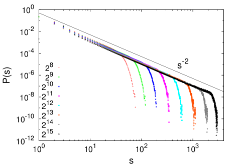
Figure 1: (Color online) The probability density $P(s)$ for fraction of restaurants with $s$ agents. The data is shown for different system sizes $N=2^{8},2^{9},2^{10},2^{11},2^{12},2^{13},2^{14},2^{15}$. The power law exponent is compared with $s^{-2}$.

Let $a_{i}(t)$ denote the number of customers on the evening $t$ in the restaurant $i$ characterized by fitness $p_{i}$ in the steady state. So, $\sum_{i}a_{i}(t)=N$. Let $n^{\prime}$ denote the average number of agents on any evening who are choosing restaurants randomly. Then, for a restaurant $i$, $a_{i}(t)p_{i}$ agents are returning to restaurant $i$ on the next evening, and an additional $n^{\prime}/N$ agents on the average additionally come to that restaurant. This gives

$$\overline{a_{i}(t+1)}=\overline{a_{i}(t)}p_{i}+n^{\prime}/N,$$ (2)

where $\overline{a_{i}}$ would now denote the average quantity. In the steady state, we have $\overline{a_{i}(t+1)}=\overline{a_{i}(t)}=\overline{a_{i}}$ and hence

$$\overline{a_{i}}(1-p_{i})=\frac{n^{\prime}}{N}$$ (3)

giving

$$\overline{a_{i}}=\frac{n^{\prime}}{N}\frac{1}{1-p_{i}}.$$ (4)

These calculations hold for large $p_{i}$ (close to $1$) which give large values of $a_{i}$ close to $\overline{a_{i}}$. Thus, for all restaurants,

$$\sum_{i}\overline{a_{i}} = N=\frac{n^{\prime}}{N}\sum_{i}\frac{1}{1-p_{i}}$$

$$\Rightarrow n^{\prime} = \frac{N^{2}}{\sum_{i}\frac{1}{1-p_{i}}}.$$ (5)

Now, let us consider a case of $\Pi(p)=1$, where $p_{i}=1-i/N$ for $i=1,2,\ldots,N$. Thus,

$$n^{\prime}=\frac{N}{\sum_{i}\frac{1}{i}}\approx\frac{N}{\ln(N+1)}$$ (6)

for large $N$. We numerically computed $P(s)$ for this particular case and the computed value of the cutoff in $P(s)$ which comes from the largest value of $p_{i}$ which is $p_{1}=1-1/N$, and it agrees nicely with our estimated Eq. 6.

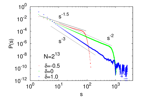
Figure 2: (Color online) The probability density $P(s)$ for fraction of restaurants with $s$ agents, for different distributions $\Pi(p)=(1+\delta)(1-p)^{\delta}$, with $\delta=-0.5,0,1.0$. The power law exponents agree with $\nu=2+\delta$. The data are shown for $N=2^{13}$.

Following Ref. Mohanty2006 , one can derive the form of the size distribution $P(s)$ easily. Since, R.H.S. of Eq. (3) is a constant ($=C$, say), $dp=da/a^{2}=ds/s^{2}$, since $a_{i}$ being the number of agents in restaurant $i$ denotes nothing but the size $s$. An agent with a particular fitness $p$ ends up in a restaurant of characteristic size $s$ given by Eq. (3), so that one can relate $\Pi(p)dp=P(s)ds$. Thus,

$$P(s) = \Pi(p)\frac{dp}{ds}=\frac{\Pi\left(1-\frac{C}{s}\right)}{s^{2}}.$$ (7)

Thus, for an uniform distribution $\Pi(p)=1$, $P(s)\sim s^{-2}$ for large $s$. It also follows that for $\Pi(p)=(1+\delta)(1-p)^{\delta}$, one should get

$$P(s)\sim s^{-(2+\delta)},\;\;\textrm{with}\;-1<\delta<\infty.$$ (8)

Thus $\nu$ does not depend on any feature of $\Pi(p)$ except on the nature of this function near $p=1$, i.e., the value of $\delta$, giving $\nu=2+\delta$.

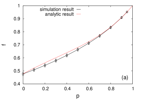
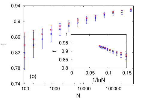
Figure 3: (Color online) Utilization fraction $f$ in the model (a) with fixed fitness $p$. The data is shown for $N=1024$. The dotted line gives the analytical estimate. (b) $f$ for the case of uniformly distributed $p$ i.e., for $\Pi(p)=1$: $p_{i}=1-i/N$ (red squares) and uniformly random (blue circles) for various system sizes $N$. The inset shows the variation of $f$ with $1/\ln N$. Error bars are also shown.

Eq. 8 can also be derived in an alternative way. The fraction of redistributed people $n^{\prime}/N$ choose $N$ restaurants randomly, and thus its distribution is Poissonian of some parameter $c$. The stationary distribution of $a_{i}$ is also Poissonian of parameter $c/(1-p_{i})$. The average distribution over $p_{i}$ can hence be computed exactly as

$$P(a) = \frac{\delta+1}{a!}\int_{0}^{1-\epsilon}dp(1-p)^{\delta}\left(\frac{c}{1-p}\right)^{a}\exp\left(-\frac{c}{(1-p)}\right)$$ (9)

$$= \frac{(\delta+1)c^{\delta+1}}{a!}\int_{c}^{c/\epsilon}u^{a-2-\delta}\exp(-u)du,$$

where $\epsilon=1/N^{\frac{1}{\delta+1}}$ is a cutoff, in particular necessary for $\delta=0$, and

$$c=\left\{\begin{array}[]{lll}\frac{1}{(\delta+1)}\int_{0}^{1-\epsilon}dp(1-p)^{\delta-1}&=\frac{\delta}{(\delta+1)},&\textrm{if}\ \delta>0,\\ \frac{1}{\log(1/\epsilon)}&=\frac{1}{\log(N)},&\textrm{if}\ \delta=0.\end{array}\right.$$ (10)

If the bounds of the above integral (Eq. 9) can be put respectively to $0$ and $\infty$, for an intermediate range of $a$ one gets

$$P(a) \sim \frac{(a-2-\delta)!}{a!}$$ (11)

$$\sim a^{-(2+\delta)},\;\;\textrm{when}\;a\gg 2+\delta,$$

which leads to the result below Eq. 8, while Eq. 8 is only valid for large $a$.

In Fig. 2 we compare the numerical simulation results for $\Pi(p)=(1+\delta)(1-p)^{\delta}$ and indeed find the agreement $\nu=2+\delta$.

At this point, it is worthwhile to mention the case when restaurants have the same fitness, $p_{i}=p$ $\forall i$. The $p=0$ case is trivial and same as our random benchmark. The size distribution $P(s)$ is Poissonian: $P(s)=\frac{1}{s!}\exp(-1)$. For $0<p<1$, $P(s)$ does not show any difference, except in the largest values of $s$. Trivially, the $p=1$ case has no dynamics. This is strikingly different from the CC model Chakraborti2000 , where the wealth distribution $P(m)$ resembles Gamma distributions Patriarca2004 , with the maxima for $\lambda=0$ at $m=0$ monotonically going to $m=1$ for $\lambda\to 1$, $m$ being calculated in units of average money per agent. However, in the limit of $g=N/R\gg 1$ (continuum limit), the above models will reproduce results of CC and CCM.

III.2 Utilization

We further assume that the restaurants prepare as many meals on a particular evening as there were customers on the previous evening. We define utilization fraction $f$ as the average fraction of agents getting food. Thus, formally,

$$f=\left\langle\overline{\frac{1}{N}\sum_{i}\min[a_{i}(t),a_{i}(t+1)]}\right\rangle,$$ (12)

where the bar means time average in the steady state and $\langle\ldots\rangle$ means ensemble average. Thus, Eq. 12 computed in the steady state will give the steady state value of utilization $f$.

Let us consider the case when the agents choose restaurants randomly. The utilization fraction $f$ is about $0.476(5)$ as computed from numerical simulations. We can provide an analytical argument for this.

The probability of finding a restaurant with exactly $m$ agents is given by

$$\pi(m)=\frac{1}{m!}\exp(-1).$$ (13)

In the steady state, $\pi(m)$ fraction of restaurants each provide $m$ meals. Then the fraction of agents not getting food can be calculated exactly, and is given by

$$1-f=\pi(0) + \pi(1)[1.\pi(2)+2.\pi(3)+\ldots]$$ (14)

$$+ \pi(2)[1.\pi(3)+2.\pi(4)+\ldots]$$

$$+ \pi(3)[1.\pi(4)+2.\pi(5)+\ldots]+\ldots$$

$$=\pi(0) + \sum_{r=1}^{\infty}\sum_{r^{\prime}=r+1}^{\infty}\pi(r)\pi(r^{\prime})(r^{\prime}-r).$$ (15)

Eq. (15) can be computed to any degree of accuracy. The series for its first four terms, i.e., keeping upto $r=3$, gives $1-f=\frac{1}{e}+\frac{1}{e^{2}}+\frac{1}{2e^{2}}(3-e)+\frac{1}{6e^{2}}\left(\frac{11}{2}-2e\right)\approx 0.523$. Thus, $f\approx 0.477$ which compares pretty well with the numerical simulations.

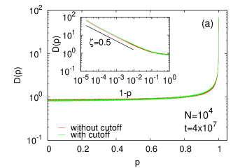
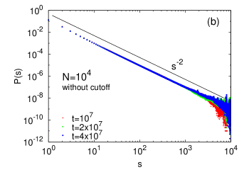
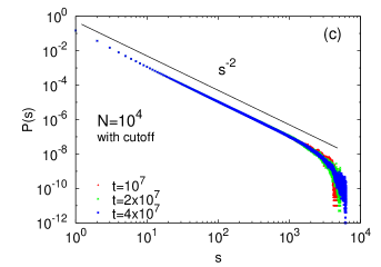
Figure 4: (Color online) (a) The distributions $D(p)$ of $p$ for Cases I (without cutoff) and II (with cutoff). The inset shows $D(p)$ vs $1-p$, and the solid line is a guide to $\zeta=0.5$. The data is shown for $N=10^{4}$. (b) The distributions $P(s)$ of $s$ for Case I (without cutoff) at different times $t=10^{7},2\times 10^{7},4\times 10^{7}$ for $N=10^{4}$. The solid line is a guide to $\nu=2$. (c) The distributions $P(s)$ of $s$ for Case II (with cutoff) at different times $t=10^{7},2\times 10^{7},4\times 10^{7}$ for $N=10^{4}$. The solid line is a guide to $\nu=2$.

However, when all restaurants have the same fitness ($=p$), the fraction of agents choosing restaurants randomly is $l=1-p$, who are mobile agents, while $1-l$ fraction of agents are immobile. Then, for this mobile fraction $l$, the probability of finding a restaurant with exactly $m$ mobile agents will be a Poissonian

$$\pi(m)=\frac{l^{m}}{m!}\exp(-l).$$ (16)

Then, we will basically have Eq. 15 with $\pi(m)$ given by Eq. 16. Thus,

$$1-F(l)=e^{-l} + (l^{2}e^{-l}-le^{-l}+le^{-2l})$$ (17)

$$+ \left(\frac{l^{3}e^{-l}}{2}-l^{2}e^{-l}+\frac{l^{3}e^{-2l}}{2}+l^{2}e^{-2l}\right)$$

$$+ \ldots,$$

where $F(.)$ is the contribution to utilization from the mobile agents. Now, the total utilization fraction will constitute of the contributions of the mobile and immobile agents:

$$f(p)=lF(l)+(1-l)=(1-p)F(1-p)+p.$$ (18)

We compute Eq. 18 upto 3 terms in the series, and plot in Fig. 3a, and compare with numerical simulations. In fact, $f(p)\to 1$ as $p\to 1$, which can easily be explained from the fact that at the limit of $p\to 1$, there is hardly any fluctuation and $a_{i}(t+1)=a_{i}(t)$ identically.

For the case when $\Pi(p)=1$, we observe that $f$ grows with system size $N$, roughly as $1-b/\ln N$, which tells us that $f\to 1$ as $N\to\infty$ (Fig. 3b). Thus, for large systems, it is possible to attain full utilization.

III.3 Evolution with fitness

Here we apply a new strategy for the model, as follows: initially all the restaurants are given the same values of $p$ and one agent per restaurant. Each day agents go to the restaurants obeying the rule as described in previous section i.e., each agent will return to the same restaurant with probability $p$ or choose any other restaurant uniformly. By this strategy, some of the restaurants will lose agents and correspondingly some will gain agents compared to previous day’s attendance. Fitness plays an important role in the evolutionary models of species (see e.g., Ref. bak1993punctuated ). Let only the restaurants which lose agents refresh their fitness $p$ by a new value randomly drawn from $\Pi(p)=(1+\delta)(1-p)^{\delta}$ in $[0,1)$ for next day. This process may actually mean that a restaurant performing badly goes out of business and is replaced by a new one. In the context of cities, this might mimic a process of city decline/death and a subsequent emergence of a new city.

We study the problem for two cases: where we do not use any cutoff for $p$ (Case I) and where a natural cutoff in $p$ is used (Case II).

Case I: $N$ restaurants are initially assigned the same value of $p$ and one agent in each restaurant, and the dynamics is as described above, but the new values of $p$ are drawn from a uniform random distribution in $[0,1)$ (i.e., $\delta=0$). The agent distribution $P(s)$ in the steady state follows a power law with exponent $\nu=2$. Also the steady state distribution $D(p)$ of $p$ in higher value of $p$ behaves as

$$D(p)=\frac{A}{(1-p)^{\zeta}}+B,$$ (19)

where $A,B$ are constants and $\zeta\simeq 0.5$, as shown in Fig. 4a. We checked numerically for several values of $\delta$ and find that the relation

$$\zeta=\delta-\frac{1}{2}$$ (20)

holds. Here we use $D(p)$ to distinguish from $\Pi(p)$, the former being generated out of the dynamics, while the latter is a pre-determined distribution.

Case II: To avoid the condensation, we use a cutoff for $p$. For $\delta=0$ we allowed the highest value for $p$ to be $1-1/N^{2}$. We choose this cutoff since $\zeta=-1/2$ near $p=1$, which gives the cutoff to be $\epsilon=1/N^{\frac{1}{1+\zeta}}=1/N^{2}$. We find that same power law behavior with an exponential cutoff. Additionally, the system is ergodic; we observe that agent distribution $P_{i}(s)$ at any randomly selected restaurant $i$ is the same as the agents distribution computed from all restaurants (see Fig. 4c). Eq. 19 and Eq. 20 still hold true.

IV Empirical evidences

In Fig. 5, we plot the size $s$ of cities, communes, municipalities and their rank $k$ according to size for several countries across the world, and one typically observes variations in the exponents. The slopes of the curves basically give the power law exponent $1/\gamma=\nu-1$ corresponding to the Zipf law. We computed these exponents at the tail of the distributions using maximum likelihood estimates (MLE) Clauset2009 and subsequently calculated $\gamma$, as shown in Table. 1.

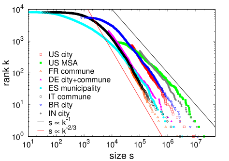
Figure 5: (Color online) Plot of size $s$ with rank $k$ of a city for different countries. The two straight lines are respectively $s\propto k^{-1}$ and $s\propto k^{-2/3}$, guides to the approximate extremes of the power law behavior of the data sets. The actual exponents of the power law fits are given in Table. 1.

Table 1: Zipf exponents for different countries, computed using MLE. For USA, we used two data sets: cities with population above $50,000$, and for Metropolitan Statistical Area (MSA). For India, data for cities with population above $100,000$ are used.

Country	Year	demarcation	$\gamma$
USA US1	2012	city population $>50,000$	0.74(2)
USA US1	2012	MSA	0.91(2)
France France	2006	commune	0.67(1)
Germany Germany	2011	city & commune	0.85(2)
Spain Spain	2011	municipality	0.77(1)
Italy Italy	2010	commune	0.77(1)
Brasil Brasil	2012	city	0.88(1)
India India	2011	city population $>100,000$	0.63(1)

V Summary and discussions

The social and economic reasons for the development of an urban agglomeration or a city batty2008size involve growth over time as well as migration, decay, as well as death, due to natural or economic (industrial) reasons. In this article we model city growth as a resource utilization problem, specifically in the context of city size distributions. Zipf law for city size distribution can be thought to be a consequence of the variation in the quality of available services, which can be measured in terms of various amenities. We argue that this measure can be characterized by an intrinsic fitness. We make a correspondence from the population in cities to the number of customers in restaurants in the framework of the Kolkata Paise Restaurant problem, where each restaurant is characterized by an intrinsic fitness $p$ similar to the difference in the quality of services in different cities. The basic model is introduced in Sec. II. In Sec. III.1, we calculate the size distributions, and in Sec. III.2, the exact value of the utilization fraction for the case when choices are made independent of fitness. Results for the case with uniform fitness are also reported there. When fitness is uniformly distributed, it can give rise to a power (Zipf) law for the number of customers in each restaurant. We investigate a variant of the model (Sec. III.3) where the fitness can be seen as the ability to stay in the business. When a restaurant loses customers, its fitness is refreshed with another random value. In the steady state, the power-law distribution of the number of customers still holds, implying the robustness of the model (with fitness distribution characterized by power laws). Using a simple mechanism in which agents compete for available resources, and find the best solution using iterative learning, we show that the emergent size distribution given by the number of customers in restaurants is a power law. It may be noted that even though we consider here the particular case of $N=R$, the possibility that the restaurants (cities) adjust (learn) their fitness according to the past experience, induce the power law distribution of the customers (Sec. III.3), leaving many restaurants (cities) vacant or dead.

Although our model, using a very simple mechanism of migration of agents in a system of cities (restaurants) with a random fitness distribution reproduces the Zipf law, we have not taken into consideration any spatial structure, the costs incurred in migration/transport of agents (cf. Ref. gastner2006spatial ), and the spatial organization of facilities um2009scaling which may emerge as important factors that drive the flow of population from one city to another. We did not incorporate several details of social organization but kept the bare essential ingredients that can give rise to Zipf law. Although our study limits to a mean field scenario, being defined on a regular, fully connected network, one can as well study the problem on directed networks chatterjee2009kinetic which takes into account the asymmetry in the flows between different nodes (cities).

- (1) C. Castellano, S. Fortunato, and V. Loreto, Rev. Mod. Phys. 81, 591 (2009).
- (2) P. Sen and B. K. Chakrabarti, Sociophysics: An Introduction (Oxford University Press, Oxford, 2013).
- (3) F. Auerbach, Petermanns Geographische Mitteilungen 59, 74 (2008).
- (4) G. K. Zipf, Human behavior and the principle of least effort. (Addison-Wesley Press, 1949).
- (5) K. Gangopadhyay and B. Basu, Physica A 388, 2682 (2009).
- (6) L. Benguigui and E. Blumenfeld-Lieberthal, Computers Envir. Urb. Sys. 31, 648 (2007).
- (7) M. E. J. Newman, Contemporary Phys. 46, 323 (2005).
- (8) X. Gabaix, Am. Econ. Rev. 89, 129 (1999).
- (9) D. H. Zanette and S. C. Manrubia, Phys. Rev. Lett. 79, 523 (1997).
- (10) M. Marsili and Y.-C. Zhang, Phys. Rev. Lett. 80, 2741 (1998).
- (11) R. L. Axtell, Science 293, 1818 (2001).
- (12) K. Okuyama, M. Takayasu, and H. Takayasu, Physica A 269, 125 (1999).
- (13) Y. Fujiwara, Physica A 337, 219 (2004).
- (14) L. M. A. Bettencourt, J. Lobo, D. Helbing, C. Kühnert, and G. B. West, Proc. Nat. Acad. Sci. 104, 7301 (2007).
- (15) Global Cities Index, http://www.atkearney.com/research-studies/global-cities-index, retreived March, 2014.
- (16) M. Batty, Nature 444, 592 (2006).
- (17) P. Beaudry, D. A. Green, and B. M. Sand, J. Urban Econ. 79, 2 (2014).
- (18) A. Chakraborti, D. Challet, A. Chatterjee, M. Marsili, Y.-C. Zhang, and B. K. Chakrabarti, Physics Reports (in press); arXiv:1305.2121 (2013).
- (19) A. S. Chakrabarti, B. K. Chakrabarti, A. Chatterjee, and M. Mitra, Physica A 388, 2420 (2009).
- (20) A. Ghosh, A. Chatterjee, M. Mitra, and B. K. Chakrabarti, New J. Phys. 12, 075033 (2010).
- (21) D. Challet, M. Marsili, and Y.-C. Zhang, Minority games: interacting agents in financial markets (Oxford Univ. Press, Oxford, 2004).
- (22) A. Ghosh, D. De Martino, A. Chatterjee, M. Marsili, and B. K. Chakrabarti, Phys. Rev. E 85, 021116 (2012).
- (23) D. Dhar, V. Sasidevan, and B. K. Chakrabarti, Physica A 390, 3477 (2011).
- (24) S. Biswas, A. Ghosh, A. Chatterjee, T. Naskar, and B. K. Chakrabarti, Phys. Rev. E 85, 031104 (2012).
- (25) V. M. Yakovenko and J. Barkley Rosser Jr, Rev. Mod. Phys. 81, 1703 (2009).
- (26) B. K. Chakrabarti, A. Chakraborti, S. R. Chakravarty, and A. Chatterjee, Econophysics of Income and Wealth Distributions (Cambridge Univ. Press, Cambridge, 2013).
- (27) A. A. Drăgulescu and V. M. Yakovenko, Eur. Phys. J. B 17, 723 (2000).
- (28) A. Chatterjee and B. K. Chakrabarti, Eur. Phys. J. B 60, 135 (2007).
- (29) A. Chakraborti and B. K. Chakrabarti, Eur. Phys. J. B 17, 167 (2000).
- (30) M. Patriarca, A. Chakraborti, and K. Kaski, Phys. Rev. E 70, 016104 (2004).
- (31) A. Chatterjee, B. K. Chakrabarti, and S. S. Manna, Physica A 335, 155 (2004).
- (32) A.-L. Barabási and R. Albert, Science 286, 509 (1999).
- (33) P. K. Mohanty, Phys. Rev. E 74, 011117 (2006).
- (34) P. Bak and K. Sneppen, Phys. Rev. Lett. 71, 4083 (1993).
- (35) A. Clauset, C. R. Shalizi, and M. E. J. Newman, SIAM Review 51, 661 (2009).
- (36) Population estimates – U.S. Census Bureau, https://www.census.gov/popest/data, retreived August, 2013.
- (37) Insee – Population, http://www.insee.fr/fr/themes/ theme.asp?theme=2, retreived August, 2013.
- (38) Census Population – Germany, http://www.citypopulation.de/php/germany-census.php, retreived August, 2013.
- (39) Población de España - datos y mapas, http://alarcos.inf-cr.uclm.es/per/fruiz/pobesp/, retreived August, 2013.
- (40) Statistiche demografiche – ISTAT, http://demo.istat.it/bil2010/index02.html, retreived August, 2013.
- (41) DATASUS, http://www2.datasus.gov.br/DATASUS/, retreived August, 2013.
- (42) Top cities of India by Population census 2011, http://www.census2011.co.in/city.php, retreived August, 2013.
- (43) M. Batty, Science 319, 769 (2008).
- (44) M. T. Gastner and M. E. J. Newman, Eur. Phys. J. B 49, 247 (2006).
- (45) J. Um, S.-W. Son, S.-I. Lee, H. Jeong, and B. J. Kim, Proc. Nat. Acad. Sci. 106, 14236 (2009).
- (46) A. Chatterjee, Eur. Phys. J. B 67, 593 (2009).