Ionizing stellar population in the disc of NGC 3310 – I. The impact of a minor merger on galaxy evolution

Abstract

Numerical simulations of minor mergers predict little enhancement in the global star formation activity. However, it is still unclear the impact they have on the chemical state of the whole galaxy and on the mass build-up in the galaxy bulge and disc. We present a two-dimensional analysis of NCG 3310, currently undergoing an intense starburst likely caused by a recent minor interaction, using data from the PPAK Integral Field Spectroscopy (IFS) Nearby Galaxies Survey (PINGS). With data from a large sample of about a hundred H ii regions identified throughout the disc and spiral arms we derive, using strong-line metallicity indicators and direct derivations, a rather flat gaseous abundance gradient. Thus, metal mixing processes occurred, as in observed galaxy interactions.

Spectra from PINGS data and additional multiwavelength imaging were used to perform a spectral energy distribution fitting to the stellar emission and a photoionization modelling of the nebulae. The ionizing stellar population is characterized by single populations with a narrow age range (2.5-5 Myr) and a broad range of masses (10⁴–6$\times 10^{6}$ M_⊙ ). The effect of dust grains in the nebulae is important, indicating that 25–70% of the ultraviolet photons can be absorbed by dust. The ionizing stellar population within the H ii regions represents typically a few percent of the total stellar mass. This ratio, a proxy to the specific star formation rate, presents a flat or negative radial gradient. Therefore, minor interactions may indeed play an important role in the mass build-up of the bulge.

1 Introduction

The friction between gas and dust in a merger event can have an important impact on the evolution of the galaxies involved. Minor mergers are usually defined as the collision between two galaxies with a mass ratio smaller than 1:3-1:4. Enhanced star formation when compared with isolated objects has been observed in samples of interacting/merging galaxies (e.g. Kennicutt et al. 1987; Barton Gillespie et al. 2003; Geller et al. 2006; Woods & Geller 2007). Numerical simulations of minor mergers indicate that they can trigger nuclear activity (Mihos & Hernquist, 1994; Hernquist & Mihos, 1995; Eliche-Moral et al., 2011), alter the morphologies of galaxies  (Robertson et al., 2006) and activate bars (Laine & Heller, 1999; Romano-Díaz et al., 2008). Contrary to major mergers, minor mergers are much less violent dynamical processes since they do not destroy the disc of the main progenitor. Nevertheless, they have been increasingly recognized as important players in galaxy evolution and, in particular, in the formation and assembly of bulges especially in lower mass systems (Guo & White 2008, Hopkins et al. 2010, and references therein). Yet, whether they are also important for the total stellar mass build-up in galaxies in general is unclear and controversial (Bournaud et al., 2007; López-Sanjuan et al., 2011; Newman et al., 2012; Xu, 2013).

The induced star formation associated with the gas motions created by an interaction or the presence of bars is also expected to have an impact in the chemical distribution of the galaxies. Inflows of metal poor gas from the outer parts of the galaxy can decrease the metallicity in inner regions and modify the radial abundance gradients across spiral discs (Rupke et al., 2010). In fact, some studies have found that interacting galaxies do not follow the well established correlation between luminosity and metallicity found in normal disc galaxies. Shallower or null metallicity gradients and relatively high metallicity H ii -like regions have been observed in the outer part of the galaxies in major merger events ( Kewley et al. 2006; Ellison et al. 2008; Michel-Dansac et al. 2008; Rupke et al. 2008; Peeples et al. 2009; Miralles-Caballero et al. 2012; Sánchez et al. 2014). A similar effect can have the action of inward and outward radial flows of interstellar gas induced by the non-axisymmetrical potential of the bars (e.g., Friedli et al. 1994; Roy & Walsh 1997 ).

There is extensive literature on the impact of a major merger event on the evolution of the involved galaxies. However, only a handful recent works have been focused on minor mergers (e.g. Krabbe et al. 2011; Alonso-Herrero et al. 2012). Therefore, more observational studies are needed to provide a deeper insight on the effect of less violent dynamical phenomena on galaxy evolution.

NGC 3310 is a very distorted spiral galaxy classified as an SAB(r)bc by de Vaucouleurs et al. (1991), with strong star formation. The star formation activity, especially a vigorous circumnuclear star-forming ring, has been studied over a wide range of wavelengths from X-rays to radio (e.g. Balick & Heckman 1981; Pastoriza et al. 1993; Zezas et al. 1998; Díaz et al. 2000; Elmegreen 2002; Hägele et al. 2010, 2013; Mineo et al. 2012). Several studies support that this galaxy collided with a poor metal dwarf galaxy, which caused a burst of star formation (Balick & Heckman, 1981; Schweizer & Seitzer, 1988; Smith et al., 1996). It has also been suggested that NGC 3310 has actually experienced several interactions with small galaxies (Wehner et al., 2006). The starburst activity of this galaxy began some 100 Myr ago (Meurer, 2000), although some of the clusters are rather young, indicating that starburst galaxies may remain in the starburst mode for quite some time. Pastoriza et al. (1993) reported that the circumnuclear regions in NGC 3310 present low metal abundances (0.2-0.4 Z_⊙), in contrast to what is generally found in early-type spirals (Díaz et al., 2007).

In order to provide a better insight on the effects of the past interaction in the disc of NGC 3310, we need to investigate the properties of the hot ionized gas and the stellar population distributed along the whole disc. Studies based on NGC 3310 have mainly been focused on the properties of the young massive population (i.e. $\tau<10$ Myr and stellar mass m_⋆ = 10⁵-10⁶ M_⊙ ) in the circumnuclear region. These studies made use of photometric images and long-slit spectroscopy, which are limited to either spectral range and/or sampling biases (i.e. area coverage, only the most luminous clusters and H ii -like regions with a very limited range in ionization conditions or only a unique aperture in large sample of galaxies, etc.). With the advent of the Integral Field Spectroscopy (IFS) such limitations can be overcome or at least significantly diminished. Nowadays, the use of IFS to perform wide-field 2D analyses of galaxies is well established and continuously growing. Large fields of view (FoV) can now be observed with simultaneous spatial and spectral coverage. We thus devised the PPAK Integral-field-spectroscopy Nearby Galaxies Survey (PINGS; Rosales-Ortega et al. 2010) in order to solve the limitations just mentioned. This is a survey specially designed to obtain complete emission-line maps, stellar populations and extinction using an IFS mosaicking imaging for nearby ($D_{\mathrm{L}}\leq$ 100 Mpc) well-resolved spiral galaxies. It takes the advantage of one of the world’s widest FoV integral field unit (IFU).

This paper focuses thus on the characterization of the ionizing population in the stellar disc of NGC 3310 so as to study the impact of the minor merger on the star formation properties of the remnant. The specific goals of this study are: (i) to obtain gaseous abundance determinations of not a handful but a non-biased luminosity hundred or so H ii regions distributed all along the disc, which are necessary to better trace radial abundance gradients; (ii) to characterize the age, mass and other star formation properties of the ionizing stellar population and (iii) to investigate the extent at which the interaction could have affected the mass growth in the disc. The PINGS data, together with retrieved multiwavelength images covering from the near-$UV$ to the near-$IR$ spectral range, are well suited to deal with these issues with unprecedented statistics. In a companion paper we will focus on the study of the Wolf–Rayet (WR) population present in the circumnuclear regions and arms in NGC 3310. The presence of this population, which has been detected in the PINGS spectra, sets important constraints on the age and nature of the most massive ionizing stellar population (i.e. M $\geq$ 40 M_⊙ ).

The paper is organized as follows. We present the data set used in Sect. 2. In Sect. 3, we describe the analysis techniques used (i.e. to identify the H ii regions, decouple the gaseous and the continuum stellar emission, to obtain the chemical abundances of the gas and to estimate the age and the mass of the ionizing stellar population) and present our abundance and stellar population property derivations for H ii regions identified in the disc of NGC 3310. We first discuss in Sect. 4 the effects due to biases and systematics of the analysis techniques. We then proceed with the scientific discussion on the radial abundance gradient in the galaxy and on the star formation properties in the disc of NGC 3310 and how they might have been affected by the past minor interaction. We finally draw our conclusions in Sect. 5. Throughout this paper, the luminosity distance to NGC 3310 is assumed to be 16.1 Mpc (taken from the NASA Extragalactic Database). With an adopted cosmology of H₀ = 73 km s^-1 Mpc^-1 an angle of 1 arcsec corresponds to a linear size of 78 pc.

2 Observations and data acquisition

2.1 PINGS data

NGC 3310 observations were carried out with the 3.5m telescope of the Calar Alto Observatory using the Postdam Multi-Aperture Spectrograph (PMAS;  Roth et al. 2005) in the PMAS fibre package mode (PPAK; Verheijen et al. 2004, Kelz et al. 2006). This was part of the PINGS (Rosales-Ortega et al. 2010). In brief, the V300 grating was used to cover the 3700-7100 Å spectral range with a spectral resolution of 10 Å, corresponding to 600 km s^-1, at $\lambda$ = 5000 Å. We took three pointings with a dithered pattern (three dithered exposures per pointing), using a mean acquisition time per PPAK field in dithering mode (including set-up + integration time) of 2$\times$600 s per dithering position. This observing strategy allowed us to re-sample the PPAK 2.7 arcsec-diameter fibre to a final mosaic with a 1 arcsec spaxel sampling and a FoV of about 148 $\times$ 130 arcsec².

The data were reduced following Sánchez (2006), and can be summarized as follows: pre-reduction, identification of the location of the spectra on the detector, extraction of each individual spectrum, distortion correction of the extracted spectra, wavelength calibration, fibre-to-fibre transmission correction, flux calibration, allocation of the spectra to the sky position, dithered reconstruction and re-sampling.

The prereduction processing was performed using standard iraf packages while the main reduction was performed using the R3D software for fibre-fed and IFS data (Sánchez, 2006). A thorough description of all the reduction and flux calibration procedures is described in Rosales-Ortega et al. (2010) and Sánchez et al. (2011).

The reduced IFS data were stored in row-stacked-spectra (RSS) files. RSS format is a 2D FITS image where the $X-$ and $Y-$ axes contain the spectral and spatial information respectively, regardless of their position in the sky. This format requires an additional file that stores the position of the different spatial elements on the sky. After reducing each individual pointing with a first-order flux calibration we built a single RSS file for the mosaic following an iterative procedure: (1) a master pointing that has the best possible flux calibration and sky extinction correction and signal-to-noise ratio (S/N) is selected; (2) the mosaic is then constructed by adding consecutive pointings following the mosaic geometry; (3) overlapping spectra are replaced by the average between the previous pointing and the new rescaled spectra (obtained by using the average ratio of the brightest emission lines found in the overlapping spectra). (4) the resulting spectra are incorporated into the final RSS file, updating the corresponding position table.

In order to obtain the most accurate absolute spectrophotometric calibration, an additional correction was performed by comparing the IFS data with available broad-band photometry in $B$, $g$ and $r$ band (see next section). The estimated spectrophotometric accuracy of the IFS mosaic is of the order of 10-15%.

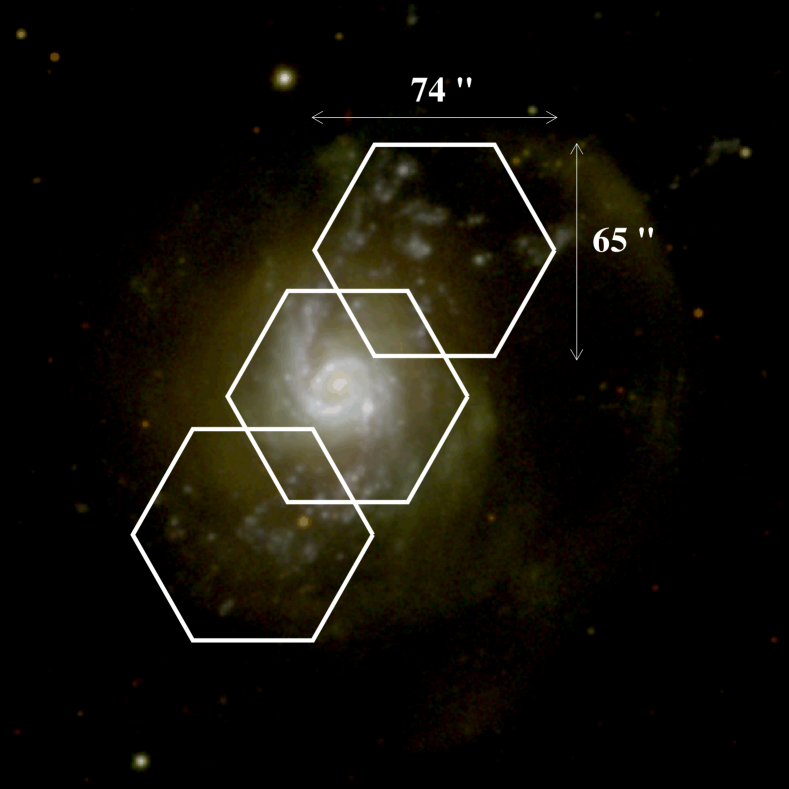
Figure 1: False colour image of NGC 3310, produced by the combination of the $u$ (in blue), $g$ (in green) and $r$ (in red) SDSS filters. Knots of star formation are clearly visible in the central region and extended outer regions. Overlaid apertures show the three pointings that were taken with PPAK, with a central position centred in the galaxy’s nucleus and two offsets of (–35, 35) and (35, –35) arcsec in (RA, Dec.) in north-west and south-east directions respectively.

A total of 8705 spectra were finally produced, spatially resolved in spaxels of 1 $\times$ 1 arcsec².

2.2 Multi-wavelength data

We retrieved publicly available broad-band imaging of this galaxy in order to perform an absolute flux re-calibration. Specifically, we used the Sloan Digital Sky Survey (SDSS) broad-band $g-$ and $r-$ filter images (with a spatial resolution of about 1 arcsec) and an $HST$ image taken with the Wide Field Planetary Camera 2 (WFPC2, with a spatial resolution of about 0.05 arcsec) using the $F439W$ filter (similar to $B$ Johnson). Although the latter does not cover the entire FoV of the galaxy, we could perform the calibration by obtaining the photometry using an aperture large enough to cover the central 30 arcsec.

We present in Fig. 1 a false colour image of NGC 3310, produced using the $u$, $g$ and $r$ SDSS filters. From the figure, it can be clearly seen that NGC 3310 is a very distorted spiral galaxy with strong star formation, with a very bright central nucleus, surrounded by a ring of luminous HII regions. Given its morphology, a tailored mosaic pattern was constructed for this galaxy (overplotted hexagons in the figure).

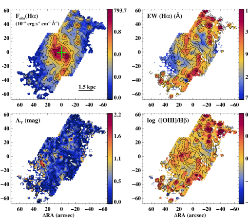
Figure 2: Maps for the observed H$\alpha$ flux, H$\alpha$ EW, $A_{V}$ extinction and [O iii]$\lambda$5007 to H$\beta$ ratio. Contours with the H$\alpha$ emission are overplotted in each case. The centre of the galaxy, which is enclosed by an H$\alpha$ peaked contour, is marked with a green plus sign. The physical scale of 1.5 kpc at the distance of the galaxy is represented by the straight line at the bottom-right corner of the first map. Axes scales are in arcsec and orientation is as usual: north up, east to the left.

We also obtained UV images of the galaxy. In particular, taken with the $UVW2$ and $UVM2$ filters (with effective wavelenghts of 2087 and 2297 Å, respectively), mounted on the OM camera onboard the XMM–Newton Satellite. The observations, with ID 0556280201, were taken in 2008. NGC 3310 was observed for more than 38 and 8 ks with the $UVW2$ and $UVM2$ filters, respectively. We reduced the observation data files using SAS version 13.0.0. The SAS script omichain was used to produce calibrated images.

The Sloan and OM ultraviolet images provide valuable information on the continuum emission of the young ionizing stellar population.

3 Analysis and results

We present here the results obtained from the analysis of the ionizing stellar population in NGC 3310 using optical IFS data together with available broad-band ancillary data.

3.1 2D general properties of the ionized gas

We study the spatially resolved distribution of the physical properties in the H ii regions of NGC 3310 by obtaining a complete 2D view of: (i) the main emission lines used in the optical range for typical abundance diagnostic methods; (ii) important spectral features useful for the analysis of the ionizing stellar populations.

In order to extract any physical information from the data set, we first need to identify the detected emission lines of the ionized gas and to decouple them from the stellar continuum. A preliminary fast decoupling was performed using an improved version of the FIT3D package (Sánchez, 2006; Sánchez et al., 2007). This software includes several routines to model and subtract the underlying stellar population of a spectral energy distribution (SED) using synthetic stellar spectra, and subsequently to fit and deblend the nebular emission lines. We refer the reader to Sánchez et al. (2007) for further details.

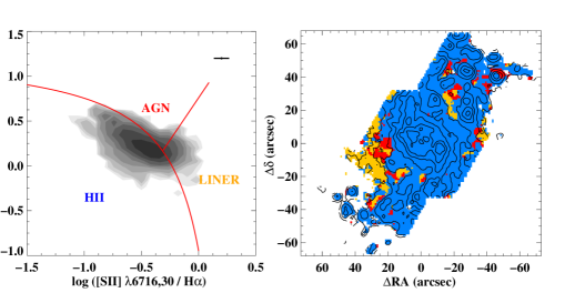
Figure 3: Left: diagnostic diagram (see text) for all the spaxels with good quality measurements. The contours show the density distribution of spaxels. The Kewley et al. (2001) red demarcation line, which is usually invoked to distinguish between star-forming regions (H ii ) and other source of ionization (AGN, LINER or composite, C), is also plotted. The error-bars at the top-right indicate the typical mean errors for the considered line ratios. Right: colour-coded maps showing the 2D spatial distribution of the ionizing source of ionization: star-forming regions (in blue), LINER or composite (in yellow) and AGN (in red).

As a result of the line fitting procedure on the stellar-subtracted (i.e. gas) spectra, a set of measured emission-line intensities was obtained for each observed spectrum of the final clean mosaic. From these sets of emission-line intensities, emission-line maps were created by interpolating the intensities derived for each individual line in each individual spectrum, based on the position tables of the clean mosaics, and correcting for the dithering overlapping effects when appropriate. The observed H$\alpha$ /H$\beta$ line ratio was used to correct the line maps for extinction, on a spaxel-by-spaxel basis. See Rosales-Ortega et al. (2010) for a full description.

We present a set of line emission maps and those with derived properties in Fig. 2. The top panel map on the left shows the 2D distribution of the H$\alpha$ observed flux. The nuclear part of the galaxy is easily identified together with the two spiral arms extending to the north and south of the galaxy. Bright inner clumps are also clearly seen within the circumnuclear region and along the whole extent of the galaxy. The lowest level contours are likely to enclose diffuse-like emission.

In practical, all regions with H$\alpha$ emission peaks, the derived EWs ($>20$ Å), as shown on the top right map, are consistent with the presence of very young (i.e. $\tau<10$ Myr) stellar populations. This is expected in H ii regions. In the nucleus, however, the relatively low values of the equivalent width (EW) distribution indicate the prevalence of the underlying old population.

We used the reddening constants from the Balmer decrement between H$\alpha$ and H$\beta$ as compared to the theoretical value for mean nebular conditions given by Osterbrock (1989) in order to estimate the reddening. We then used the law by Cardelli et al. (1989), assuming $R_{V}=3.1$, in order to correct the emission-line fluxes. The distribution of dust extinction (lower left map) although somewhat clumpy, is typically low ($A_{V}<1$ mag). In fact, the average extinction derived from the map corresponds to $\overline{A_{V}}=0.35\pm 0.31$ mag. The extinction peaks up to about $A_{V}>2$ mag only in the nucleus and along some diffuse-like emission areas.

We also show the 2D distribution of the emission-line ratio log ([O iii]$\lambda 5007$/H$\beta$ ), a parameter sensitive to the excitation, which correlates with the effective temperature of the exciting stars (Hunter, 1992). The range sampled generally lies between 0 and about 0.6, which shows that the ionized gas excitation in this galaxy is not very high. As mentioned in the introduction, NGC 3310 is a very distorted spiral galaxy with strong and rather complex star formation, very likely undergoing a merger-driven global starburst (Smith et al., 1996; Kregel & Sancisi, 2001; Wehner et al., 2006). It is widely known that massive stellar populations as young as about less than 10 Myr (i.e. hot OB stars) can well be responsible for the ionization observed in galaxies. The identification of the main ionizing mechanism in an observed object can be relatively well accomplished by the use of the so-called diagnostic diagrams (Baldwin et al. 1981, Veilleux & Osterbrock 1987). They usually involve two or three strong emission lines (SEL) that depend on the ionization degree and, to a lesser extent, on electron temperature or abundance. Fig. 3 (left) shows a common diagnostic diagram (log [O iii]/H$\beta$ versus log [S ii]$\lambda\lambda$6717,6731/H$\alpha$ ) as derived for each spaxel. Colour-coded maps were also created (Fig. 3, right) so as to spatially identify the regions ionized by different physical processes. As shown in the figure, the vast contribution of the ionization in this galaxy comes from young massive stars (H ii -like ionization). There are only a few regions (mainly not associated with H$\alpha$ peaks) associated with other ionization mechanisms, though with larger uncertainties in the determination of their emission-line ratios. This paper focuses on the ionizing stellar population. Thus, with these maps we can guarantee that our study on H ii regions in NGC 3310 is not perceptibly contaminated by other sources of ionization.

3.2 Identification of H ii regions and star–gas decoupling

The detection and segregation of H ii regions, and subsequent extraction of the spectra for each of them, was performed using the semi-automatic procedure HIIexplorer (Sánchez et al. 2012). A segmentation map that identifies each detected H ii region is provided by the code, together with the corresponding extracted spectra. In our case, a total of 99 H ii regions were identified. Fig. 4 shows the segmentation map overplotted on the H$\alpha$ map (left) and the identification of each ionizing region (right). The regions have typical radii of about 2–3 arcsec, similar to, or somewhat larger than the spatial resolution of the instrument. This translates into radii in the range of 150–250 pc, within the size range of extragalactic giant H ii regions (Kennicutt 1984; Oey et al. 2003; Hunt & Hirashita 2009; Lopez et al. 2011). Table LABEL:table:hii_catalogue reports a catalogue with the main observed properties of the identified H ii regions in NGC 3310.

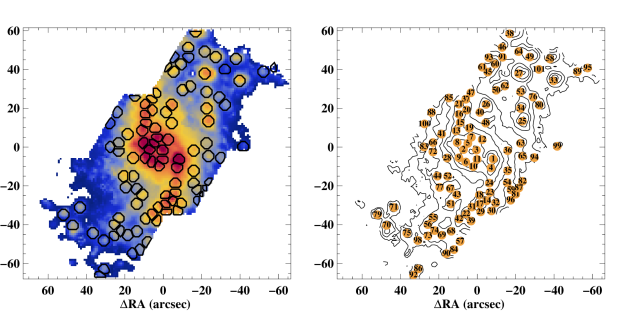
Figure 4: Left: H$\alpha$ intensity map in arbitrary units with the apertures of the identified H ii regions from the HIIexplorer routine. Right: H$\alpha$ contour map showing the spatial 2D distribution of the identified H ii regions with their identification number (HII ID in tables).

As mentioned before, particular care has always been taken in subtracting the stellar continuum so as to correctly decouple the stellar continuum from the nebular line emission. When the analysis was carried out in a spaxel-by-spaxel basis, an optimized fast analysis aimed at obtaining the best polynomial fit to the data (not necessarily giving a meaningful physical solution) was done. For the H ii regions we made use of the spectral synthesis code starlight (Cid Fernandes et al. 2004; Cid Fernandes et al. 2005). This code mixes computational techniques originally developed for empirical population synthesis with ingredients of evolutionary synthesis models. Briefly, an observed spectrum is fitted with a combination of N simple stellar populations from a set of evolutionary synthesis models. Extinction by foreground dust is also modelled by the V-band extinction $A_{V}$ . Line-of-sight (LOS) stellar motions are modelled as well, but given the rather low spectral resolution of the PINGS data ($\sim$ 600 km s^-1), off-set velocities and stellar velocity dispersions were set to a fixed default value which in any case does not affect our results since we do not intend to study the kinematics of this galaxy.

Basically, four inputs are needed for starlight : the observed spectrum, a configuration file, a mask-file to mask emission lines and a file that allocates the base spectra (i.e. the set of evolutionary synthesis models). In our analysis we made use of a compilation of a few hundreds of synthesis models covering metallicities from Z${}_{\odot}/200$ to $1.5\times\mathrm{Z}_{\odot}$ and ages from 1 Myr to 17 Gyr. This set compiles models of González Delgado et al. (2005) for $\tau<$ 63 Myr with the MILES library (Vazdekis et al., 2010, as updated by Falcón-Barroso et al. 2011) for larger ages. The models are based on the Salpeter initial mass function (IMF) and the evolutionary tracks by Girardi et al. (2000), except for the youngest ages (i.e. $\tau=$ 1-3 Myr), which are based on Geneva tracks (Schaller et al. 1992, 1993; Charbonnel et al. 1993).

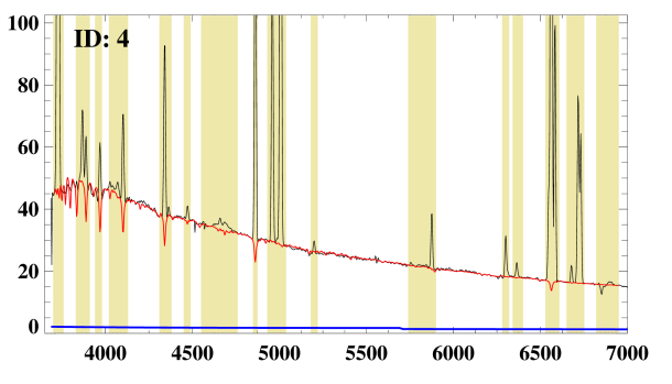
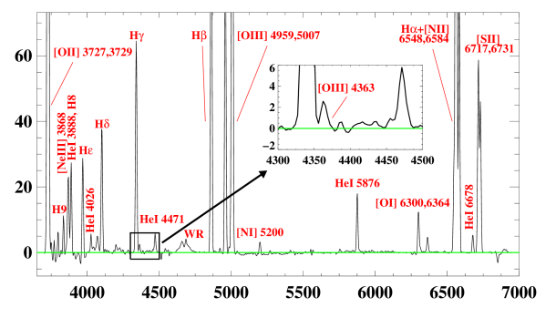
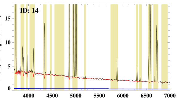
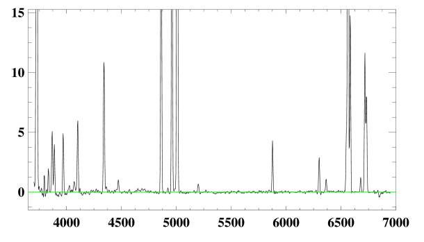
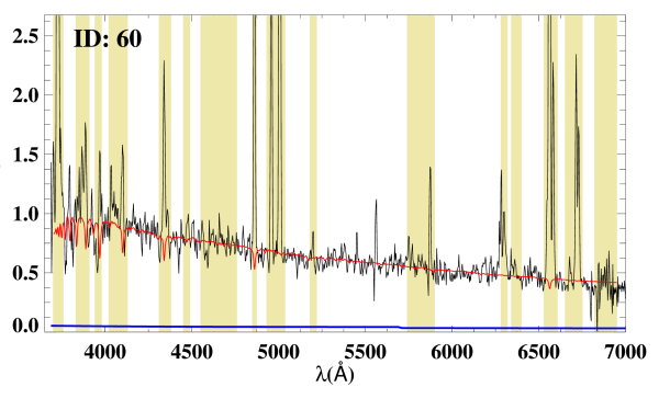
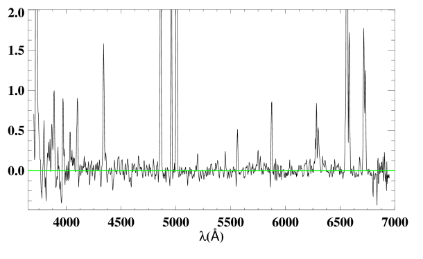
Figure 5: Left-hand panel: example of rest-frame observed spectra of three different H ii regions (left). Blue line shows the derived nebular continuum (subtracted before starlight is run) and red line shows the continuum starlight fit (C_fit). Yellowish shaded areas correspond to masked spectral intervals where typical nebular and stellar (i.e. WR) features are not included in the model libraries (i.e. blue WR bump). Masked intervals are not used in the fit. Right-hand panel: corresponding residual gas spectrum (= observed – C_fit – nebular spectrum) for each H ii region. Typical emission lines and the WR bump are labelled on the plot at the top of the panel. Inset plot there shows a zoom of the [O iii]$\lambda$4363 auroral line whereabouts in the spectrum.

The observed spectrum was not used as an input for starlight . Although the model templates used have enough spectral resolution to deal with our spectra, those corresponding to the ionizing population (i.e. $\tau\leq$ 10 Myr) lack the nebular emission component. The contribution of this component can be significant in massive H ii regions. We thus first subtracted a “nebular continuum spectrum” from each observed spectrum. This nebular spectrum was computed using the derived H$\alpha$ luminosity for each region, assuming a metallicity of Z_⊙/3, following the procedure explained in Mollá et al. (2009) and Martín-Manjón et al. (2010). That particular metallicity was chosen because it is consistent with the gaseous abundances reported in Pastoriza et al. (1993). It is also compatible with our derived metallicities (see Sect. 3.3.3). Note that this continuum can be underestimated if the H$\alpha$ luminosity is underestimated (i.e. if photon leakage or absorption by UV photons by dust grains is important).

Fig. 5 shows three examples of the fitted continuum spectrum (in red, left-hand panels) and the residual gas spectrum (right-hand panels) for H ii regions with high and low S/N. As can be seen, the nebular continuum spectrum (in blue, left-hand panels) can contribute significantly to the measured emission (in region ID 14, this continuum represents about 25% of the observed light at the reddest wavelengths). Although the residual spectrum has been identified as emission from ionized gas, sometimes a spectral feature centred around 4680 Å can be observed. This stellar spectral feature, easily recognizable in the figure for the H ii region with ID 4, corresponds to the blue WR bump and indicates the presence of WR stars.

Once starlight is run, the contribution in light and in mass of the base spectrum that best fits the input spectrum is provided as a result. In general, less than 20-30 populations are needed to fit our spectra, where normally a handful of young populations dominates the luminosity and a handful of old populations dominates the mass (see examples in Fig. 6). In order to assess the accuracy of the continuum subtraction, the code was run a hundred times for each H ii region spectrum.

Once the analysis with starlight is done, the continuum and gas spectra are decoupled, as in Sect. 3.1, though this time for the stacked spectra of the identified H ii regions, rather than for spectra of individual spaxels. Individual emission-line fluxes were then measured by considering spectral window regions of $\sim$ 200 Å. We produced idl routines to perform a simultaneous fitting of several emission lines within the spectral window with Gaussian functions. Only one spectral component is observed for each line (if different components exist, the difference in velocity must be below the spectral resolution of the data, $\sim$ 600 km s^-1). This was done for each of the 100 cleaned gas spectra for each H ii region. The statistical errors associated with the observed emission were computed taking into account: (1) the measuring method, given by the fitting and (2) the following expression:

$$\sigma_{\mathrm{l}}=\sigma_{c}N^{1/2}\left[1+\frac{\mathrm{EW}}{\mathrm{N}\Delta}\right]^{1/2}$$ (1)

where $\sigma_{\mathrm{l}}$ is the error in the observed line flux, $\sigma_{c}$ refers to the standard deviation in a box near the measured emission line, $N$ is the number of pixels used in the measurement of the line flux, EW is the line EW and $\Delta$ is the wavelength dispersion in Å pixel^-1 (Gonzalez-Delgado et al., 1994). The first term represents the error introduced in placing the continuum level and the second term scales the S/N of the continuum to the line. As a conservative approach, the maximum value between both error estimates was considered. For a given line, we took the median of the computed error and flux line of the 100 spectra as the adopted values for each H ii region, respectively. Adopted line intensities of the H ii regions are reported in Table LABEL:table:hii_catalogue.

We performed a sanity test to ensure that no overcorrection was done on the absorption stellar features. For instance, if the fitted old population is such that the H$\beta$ absorption is too strong, the obtained ratio H$\alpha$ /H$\beta$ may well be (within errors) below its theoretical value in case of no dust extinction (i.e. H$\alpha$ /H$\beta$ = 2.86, assuming case B recombination; Osterbrock 1989). This test is described in Sect. 4.1.

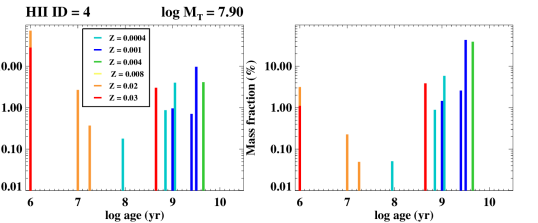
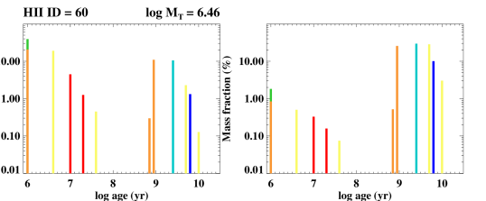
Figure 6: Examples of light- (left) and mass- (right) weighted populations obtained with on run of the STARLIGHT fitting procedure for two identified H ii regions in NGC 3310. Different colours represent different stellar metallicities ($Z$). The derived total mass, in log and solar units (log M_T), is also shown.

Table 1: Identified circumnuclear H ii regions in NGC 3310 in previous studies.

HII	ID	$L$ (H$\alpha$)	$L$ (H$\alpha$)	EW (H$\beta$)	EW (H$\beta$)	$c$ (H$\beta$)	$c$ (H$\beta$)
ID	H10		H10		H10		H10
1+4	J	554 $\pm$ 55	573	55.6 $\pm$ 0.9	82.5	0.10 $\pm$ 0.05	0.23
3	N	161 $\pm$ 16	113	10.3 $\pm$ 0.2	11.0	0.14 $\pm$ 0.03	0.42
5	R4	137 $\pm$ 13	144	26.1 $\pm$ 0.3	32.4	0.08 $\pm$ 0.03	0.23
7	R5+R6+S6	130 $\pm$ 13	193	22.5 $\pm$ 0.2	16.7	0.09 $\pm$ 0.03	0.24
8	R1+R2	219 $\pm$ 21	102	43.4 $\pm$ 0.3	28.6	0.28 $\pm$ 0.02	0.23
11	R10+R11	108 $\pm$ 10	102	15.6 $\pm$ 0.2	9.7	0.05 $\pm$ 0.03	0.23
12	R7	95 $\pm$ 9	45	13.8 $\pm$ 0.2	19.4	0.00 $\pm$ 0.01	0.17
Notes. H$\alpha$ luminosities are in 1038 erg s-1 and EWs in Å.

H ii regions detected in previous studies (Hägele et al. 2010; hereafter, H10) have been identified and the H$\alpha$ extinction-corrected luminosities, H$\beta$ EWs and extinction coefficients c(H$\beta$) are compared in Table 1. Some discrepancies are found, very likely due to the different angular resolution and aperture among the different studies (e.g., Pastoriza et al. 1993; Díaz et al. 2000; see footnotes in the table).

3.3 Chemical abundance properties of the H ii regions in NGC 3310

With our sample of H ii regions we can investigate the radial distribution of the oxygen abundance in NGC 3310 with better statistics than works based on samples of a few number of H ii regions, basically due to the limitations on the use of slits.

3.3.1 Direct oxygen abundance determination

In principle, recombination lines (i.e. O ii $\lambda$4649, $\lambda$4089) would provide the most accurate determination of the abundance, due to their weak dependence on nebular temperature. However, these lines are very faint and most of the observed emission in nebulae correspond to collisionally excited lines (CEL), whose intensities depend exponentially on the temperature. The electron temperature of the gas is useful as an abundance indicator since higher chemical abundances increase nebular cooling, leading to lower H ii region temperatures. This temperature can be determined from the ratios of auroral lines like [O iii]$\lambda$4363 to lower excitation lines such as $\lambda\lambda$4959,5007, or [N ii]$\lambda$5755 to $\lambda\lambda$6548,6584. Methods that rely on the measurements of these lines in order to obtain the abundance are the so-called direct methods.

Table 2: Direct abundance estimates of H ii regions

H ii	$I(\lambda$4636)	$t_{\mathrm{e}}$ [O iii]$\lambda$4363 $\equiv t_{3}$	$n_{\mathrm{e}}$	$t_{2}~{}(t_{3})$	12+ log (O/H)	$I(\lambda$5755)	te [N ii]$\lambda$5755	O+/H+	O2+/H+	12+ log (O/H)
ID		($\times$104) K	(cm-3)	($\times$104 K)			($\times$104 K)			($t_{3}$,$t_{\mathrm{e}}$ [N ii]$\lambda$5755)
(1)	(2)	(3)	(4)	(5)	(6)	(7)	(8)	(9)	(10)	(11)
1	1.37$\pm$ 0.30	0.97$\pm$ 0.06	108$\pm$ 8	1.00$\pm$ 0.06	8.30$\pm$ 0.10	0.74$\pm$ 0.13	1.04$\pm$ 0.08	7.96	7.96	8.26$\pm$ 0.08
4	1.52$\pm$ 0.24	1.03$\pm$ 0.05	115$\pm$ 8	1.03$\pm$ 0.06	8.23$\pm$ 0.08	0.64$\pm$ 0.12	0.95$\pm$ 0.06	8.19	7.82	8.34$\pm$ 0.09
5	1.93$\pm$ 0.29	1.12$\pm$ 0.05	123$\pm$ 17	1.09$\pm$ 0.05	8.09$\pm$ 0.07	…	…	…	…	…
7	1.70$\pm$ 0.33	1.13$\pm$ 0.07	90$\pm$ 21	1.13$\pm$ 0.06	8.03$\pm$ 0.08	0.89$\pm$ 0.18	1.01$\pm$ 0.08	8.02	7.60	8.16$\pm$ 0.12
8	1.84$\pm$ 0.42	1.08$\pm$ 0.07	112$\pm$ 18	1.07$\pm$ 0.06	8.17$\pm$ 0.10	0.79$\pm$ 0.11	1.00$\pm$ 0.05	8.08	7.76	8.25$\pm$ 0.08
13	1.51$\pm$ 0.35	1.07$\pm$ 0.07	77$\pm$ 16	1.10$\pm$ 0.06	8.12$\pm$ 0.10	1.19$\pm$ 0.11	1.17$\pm$ 0.05	7.81	7.69	8.06$\pm$ 0.06
14	1.64$\pm$ 0.36	0.96$\pm$ 0.06	37$\pm$ 6	1.07$\pm$ 0.07	8.30$\pm$ 0.10	…	…	…	…	…
15	1.98$\pm$ 0.33	1.14$\pm$ 0.06	52$\pm$ 20	1.19$\pm$ 0.05	8.02$\pm$ 0.06	0.89$\pm$ 0.14	1.04$\pm$ 0.07	8.03	7.64	8.18$\pm$ 0.09
16	2.03$\pm$ 0.34	1.17$\pm$ 0.06	108$\pm$ 24	1.13$\pm$ 0.05	8.07$\pm$ 0.07	1.10$\pm$ 0.22	1.19$\pm$ 0.12	7.81	7.59	8.02$\pm$ 0.11
19	2.23$\pm$ 0.46	1.35$\pm$ 0.11	174$\pm$ 64	1.16$\pm$ 0.05	7.96$\pm$ 0.06	…	…	…	…	…
20	2.61$\pm$ 0.45	1.29$\pm$ 0.08	109$\pm$ 48	1.21$\pm$ 0.05	7.95$\pm$ 0.05	…	…	…	…	…
21	2.46$\pm$ 0.35	1.27$\pm$ 0.07	116$\pm$ 38	1.19$\pm$ 0.05	7.99$\pm$ 0.05	1.26$\pm$ 0.25	1.27$\pm$ 0.13	7.74	7.46	7.93$\pm$ 0.12
22	2.18$\pm$ 0.48	1.05$\pm$ 0.07	34$\pm$ 15	1.15$\pm$ 0.07	8.16$\pm$ 0.09	…	…	…	…	…
26	1.63$\pm$ 0.34	1.06$\pm$ 0.06	52$\pm$ 14	1.12$\pm$ 0.06	8.12$\pm$ 0.09	…	…	…	…	…
27	3.68$\pm$ 0.47	1.17$\pm$ 0.05	92$\pm$ 25	1.15$\pm$ 0.05	8.12$\pm$ 0.05	…	…	…	…	…
32	2.11$\pm$ 0.47	1.05$\pm$ 0.07	14:	1.21$\pm$ 0.10	8.12$\pm$ 0.09	…	…	…	…	…
Notes. Col (1): H ii region identification number. Col (2): reddening-corrected flux of the [O iii]$\lambda$4363 auroral line with respect to H$\beta$ , normalized to H$\beta$ = 100. Col(3): direct determination of the electron temperature of [O iii]. Col (4): derived electron density. Col (5): derived electron temperature of [O ii], assuming that $t_{\mathrm{e}}$ ([O ii]) $\sim$ $t_{\mathrm{e}}$ ([N ii]) and the theoretical relation between $t_{\mathrm{e}}$ ([O ii]) and $t_{\mathrm{e}}$ ([O iii]) as prescribed in Pérez-Montero & Díaz (2003) (Eq. 2). Col (6): derived oxygen abundance with a direct-temperature determination of [O iii]. Col (7): reddening-corrected flux of the [N ii]$\lambda$5755 auroral line with respect to H$\beta$ , normalized to H$\beta$ = 100. Col (8): direct determination of the electron temperature for [N ii]. Col (9): O+ ionic abundance, derived using both direct determinations of the electron temperature of [O iii] and [N ii]. Col (10): same as in col. (9), but for the O2+ ion. Col. (11): derived oxygen abundance using both direct determinations of the electron temperature of [O iii] and [N ii].

We measured the auroral line [O iii]$\lambda$4363 with a detection level of S/N $>$ 4 from the “residual” gas spectra of 16 H ii regions. We refer the reader to Sect. 4.2, where we argue about the systematics introduced when measuring this line on the observed spectrum. The determination of the electron temperature ($t_{\mathrm{e}}$) and other physical conditions of the gas such as the electron density ($n_{\mathrm{e}}$, in cm^-3), and the ionic abundances were obtained using the procedures outlined in Pérez-Montero et al. (2007) and Hägele et al. (2008). We have assumed two distinct layers of ionization for each H ii region: a high ionization zone (He ii, [O iii], [NeIII], etc.) and a low ionization zone ([O ii], [N ii], [S ii], etc.), whose electron temperatures are given by $t_{3}$ and $t_{2}$, respectively.

Different prescriptions can be found in the literature that relate the $t_{3}$ and the $t_{2}$ temperatures. In our case, the $t_{2}$ temperature was determined using photoionization models that take into account the dependence on the electron density (Pérez-Montero & Díaz, 2003; Pérez-Montero & Contini, 2009):

$$t_{2}\equiv t_{\mathrm{e}}(\textrm{[{O\,{{ii}}}]})=\frac{1.2+0.002n_{\mathrm{e}}+4.2/n_{\mathrm{e}}}{t_{3}^{-1}+0.08+0.003n_{\mathrm{e}}+2.5/n_{\mathrm{e}}},$$ (2)

where the electron density was determined from the [S ii]$\lambda\lambda$6717,6731 doublet.

In a few cases the [N ii]$\lambda$5755 line was also detected and measured. In those cases, we could derive the temperature of [N ii], the temperature of the low ionization zone.

The ionic abundances were calculated based on the functional forms provided by Hägele et al. (2008), who published a set of equations for the determination of oxygen abundances in H ii regions based on a five-level atom model:

$$12+\textrm{log(O}^{2+}/\textrm{H}^{+}) \mspace{-20.0mu}=~{} \textrm{log}(\textrm{[{O\,{{iii}}}]}\lambda\lambda 4959,5007/\textrm{H}\beta)+6.144~{}+$$ (3)

$$\mspace{-90.0mu}+1.251/t_{3}-0.55\textrm{log}t_{3}$$

$$12+\textrm{log(O}^{+}/\textrm{H}^{+}) \mspace{-20.0mu}=~{} \textrm{log}(\textrm{[{O\,{{ii}}}]}\lambda\lambda 3727,3729/\textrm{H}\beta)+5.992~{}+$$ (4)

$$\mspace{-90.0mu}+1.583/t_{2}-0.681\textrm{log}t_{2}+\textrm{log}(1+0.00023n_{\mathrm{e}})$$

Finally, the total oxygen abundance was obtained assuming that

$$\frac{\textrm{O}}{\textrm{H}}=\frac{\textrm{O}^{+}}{\textrm{H}^{+}}+\frac{\textrm{O}^{2+}}{\textrm{H}^{+}}$$ (5)

Auroral line measurements, electron density and temperatures, along with the derived oxygen abundances using the methodology described in this section are reported in Table 2. With typical electron densities of the order of 100 cm^-3 and typical electron temperatures of the order of 10000 K, the derived direct abundances are subsolar, in the range 8 $\lesssim$ 12 + log(O/H) $\lesssim$ 8.3.

3.3.2 Strong-line methods

The ratios used in direct methods involve the detection and measurement of at least one intrinsically weak line, which in objects of low excitation and/or low surface brightness, often result too faint to be observed. Given these limitations, strong-line methods based on the use of strong, easily observable, optical lines have been developed throughout the years. Several abundance calibrators have been proposed involving different emission-line ratios and have been applied to determine oxygen abundances in objects as different as individual HII regions in spiral galaxies, dwarf irregular galaxies, nuclear starbursts and emission-line galaxies. By far, the most commonly strong-line calibrator used is the ratio ([O ii]$\lambda$3727 + [O ii]$\lambda\lambda$4959, 5007)/H$\beta$ , known as the $R_{23}$ method (Pagel et al., 1979). However, it is known to present many problems basically because it is double valued with a wide transition/turn-over region (12+log(O/H) $\sim$ 8.0–8.3). Furthermore, a few observed circumnuclear H ii regions in NGC 3310 are known to have a moderately low metallicity (12+log(O/H) $\sim$ 8–8.3; Pastoriza et al. 1993), just in the middle of the turn-over region of the calibrator. The spectral range covered by the PINGS data allows us, nevertheless, to employ more up-to-date strong-line calibrations that make use of more information via strong nitrogen and/or sulphur lines. This are as follows.

• 

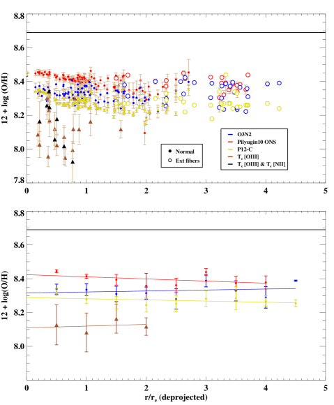
  Figure 7: Top: radial distribution of oxygen abundance in NGC 3310. $X-$ axis shows the deprojected radial distance. Different colours refer to different methods use to derive the oxygen abundance (see legend). Estimates from spectra obtained with data within the hexagonal PPAK FoV are plotted in solid symbols (either circles or triangles, the latter referring to $t_{\mathrm{e}}$-based estimates), whereas an open symbol means that the spectra were obtained from external fibres (see text). The horizontal line highlights the position of the solar abundance of 12 + log(O/H) = 8.69 (Asplund et al., 2009) in the diagram. Bottom: data have been grouped in distance bins of 0.5$r$$r_{\mathrm{eff}}$ and median values have been plotted. The error bars represent the dispersion within a given bin. The lines show a straight line fitted to the median values. We have not grouped the estimates derived from T_e-based methods that use both the auroral [O iii]  and [N ii] lines due to the lack of data.

• $O3N2$-parameter calibrations – The $O3N2$ parameter, first introduced by Alloin et al. (1979), depends on two SEL intensity ratios:

  $$O3N2=\textrm{log}\left(\frac{\textrm{[{O\,{{iii}}}]}\lambda 5007}{\textrm{H}\beta}\times\frac{\textrm{H}\alpha}{\textrm{[{N\,{{ii}}}]}\lambda 6584}\right)$$ (6)

  This parameter is almost independent of either reddening correction or flux calibration. Several calibrations using this parameter have been defined (e.g., Pettini & Pagel 2004; Pérez-Montero & Contini 2009). Recently, Marino et al. (2013) have provided an improved calibration using the largest compilation so far of temperature-based abundance determinations, and has proved its validity for 12 + log(O/H) $>8.1-8.2$ with a dispersion somewhat lower than 0.2 dex.

• ONS calibration – This calibration (Pilyugin et al., 2010) is based on several strong-line-intensity ratios to H$\beta$ from several species, including oxygen, nitrogen and sulphur as

  $$R_{2}=\textrm{[{O\,{{ii}}}]}\lambda\lambda 3727,3729/\textrm{H}\beta$$

  $$R_{3}=\textrm{[{O\,{{iii}}}]}\lambda\lambda 4959,5007/\textrm{H}\beta$$ (7)

  $$N_{2}=\textrm{[{N\,{{ii}}}]}\lambda\lambda 6548,6854/\textrm{H}\beta$$

  $$S_{2}=\textrm{[{S\,{{ii}}}]}\lambda\lambda 6717,6731/\textrm{H}\beta$$

  It uses the excitation parameter, ($P=R_{3}/(R_{3}+R_{2})$), that takes into account the effect of the ionization parameter. This calibration was derived using a set of H ii regions with measured electron temperatures.

• C-method – The ‘counterpart’ method, P12-C (Pilyugin et al., 2012), is based on the standard assumption that H ii regions with similar intensities of SEL have similar physical properties and abundances. Given all the problems that different calibrations have (e.g., different branches, different applicability ranges, the no one-to-one correspondence between oxygen and nitrogen abundances) the authors propose a method that does not know a priori in which metallicity interval (or on which of the two branches) the H ii region is located. This calibration basically selects a number of reference (well-measured abundances) H ii regions and then the abundances in the target H ii region are estimated through extra-/interpolation. According to the authors, if the errors in the line measurements are within 10%, then one can expect that the uncertainty in the C-based abundances is not in excess of 0.1 dex (although it can reach 0.15–0.2 dex in the interval 7.8 $<$ 12 + log(O/H) $<$ 8.2).

We made use of the calibrations outlined in order to search for any radial abundance gradient trend in NGC 3310 within dispersions of 0.1-0.2 dex, though larger systematic offsets can be expected from the results obtained from one calibration to another.

3.3.3 Radial abundance gradients

We have only a limited sub-sample of H ii regions with reliable $t_{\mathrm{e}}$-based abundance determinations. We thus derived abundances for almost all identified H ii regions using the strong-line calibrations described in previous sections. Fig. 7 shows the radial distribution of the oxygen abundance in NGC 3310 up to about four effective radii ($r_{\mathrm{eff}}$ ). At the assumed distance of this galaxy ($D_{\mathrm{L}}$ = 16.1 Mpc), this distance corresponds to about 11 kpc. We identify $r_{\mathrm{eff}}$ as the half-light radius, which was determined using galfit, version 3.0 (Peng et al., 2010), on the $g$-band SDSS image. Either assuming a typical Sérsic (letting the index $n$ vary) + an exponential disc profiles or a rotating Sérsic (simulating the spiral arms) + an exponential disc profiles, the resulting $r_{\mathrm{eff}}$ is around 35 arcsec (i.e. $\sim 2.5$ kpc).

For this part of the study, we have included in our catalogue spectra corresponding to the external fibres of the PPAK module (normally used to determine the local sky, grouped in bundles at $\sim$75 arcsec from the centre of the PPAK module) which show evident H ii -like emission with coincident redshift of that of NGC3310, i.e. fortuitous observations of H ii regions at very large galactocentric distances. Their 2D spatial distribution is shown in Fig. 8. In many cases, given the dithering used, the flux of 2 or 3 fibres could be integrated to obtain each spectrum of these ‘external’ regions. Although the S/N of the continuum is generally very low, the emission lines are clearly detected. The extinction corrected line intensities are reported in Table 6. These additional regions allow us to investigate if there is any abundance radial gradient in this galaxy up to more than 10 kpc. If this data set is not included we still can sample H ii regions within about 5 kpc or about 2.8$r_{\mathrm{eff}}$ . Several interesting aspects can be inferred from the plot as follows.

1. All computed gaseous abundances are sub-solar, spanning the range 7.95 $<$ 12 + log(O/H) $<$ 8.45 (between a half and a fifth solar).

2. All computed abundances using strong-line calibrations agree within 0.1–0.15 dex, covering a typical range 12 + log(O/H) = 8.2–8.4. This is expected, since the accuracy of strong-line calibrations (0.1–0.2 dex), not included in the error bars, is of the order of this range.

3. In practice, we have obtained $t_{\mathrm{e}}$-based estimates within one $r_{\mathrm{eff}}$ . Their range span oxygen abundances between 8 and 8.3 with a larger dispersion than those computed with strong-line calibrations. In general, the $t_{\mathrm{e}}$-based estimates are also lower by about 0.2–0.3 dex. With a sample of 16 H ii regions with direct abundance estimates and over 100 regions with strong-line estimates we can assure that the offset is not due to lack of statistics. In Sect. 4.2, we discuss on this disagreement.

   

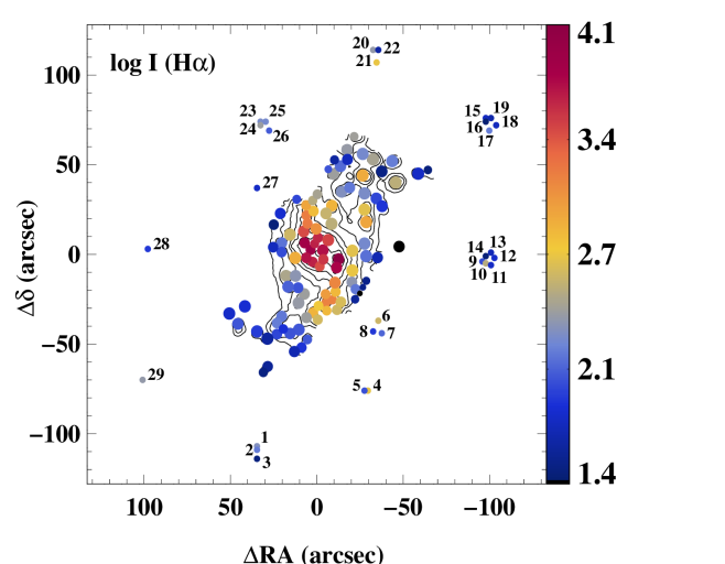
   Figure 8: H$\alpha$ contour map showing the spatial 2D distribution of the identified H ii regions and the external regions (with their identification number). While the size of the circles for the identified H ii regions represents approximately their actual size, that for the external regions corresponds to their average size. The circles are colour coded following the logarithm of the H$\alpha$ intensity in units of 10^-16 erg s^-1 cm^-2.

4. With a sample of over 100 H ii regions we do not see a clear abundance gradient in NGC 3310, further than 10 kpc away from the nucleus. A weak gradient might be present from the centre and up to 2$r_{\mathrm{eff}}$ (5 kpc). We have computed the Spearman correlation coefficient for $r<2$$r_{\mathrm{eff}}$ and have obtained a possible correlation for abundances that were derived using the ONS and the P-12C calibrations ($r=0.63,0.72$, respectively). The derived slopes of the fit are 0.06 and 0.05 dex/$r_{\mathrm{eff}}$ ($\sim$ 0.02 dex/kpc), respectively. Should an abundant gradient exist, it is significantly flatter than the observed gradients in galactic discs (i.e. $\sim$ -0.08 dex/kpc; Vilchez et al. 1988; Kennicutt & Garnett 1996; Rosolowsky & Simon 2008; Costa & Maciel 2010) and the universal gradient proposed in Sánchez et al. (2014) (i.e. $\sim$ -0.10 dex/$r_{\mathrm{eff}}$ ). For abundances obtained using the $O3N2$ calibration and the direct method (using the [O iii]$\lambda$4363 emission line), the data are not correlated, according to the Spearman’s rank- order correlation test. Besides, the intrinsic dispersion of strong-line calibrations is typically 0.1–0.2 dex. All facts considered, we conclude that either the abundance gradient of the gas in the disc of NGC 3310 is flat or at least significantly flatter than gradients observed in spirals.

3.4 Characterization of the ionizing stellar population

With the spectral information provided with the IFU data and available public wide-band imaging we can perform a detailed study on the ionizing stellar populations in NGC 3310. In particular, the line flux ratios, the EW measurements and broad-band UV and optical images help us to tightly constrain the mass and the age of the ionizing stellar populations present in the H ii regions.

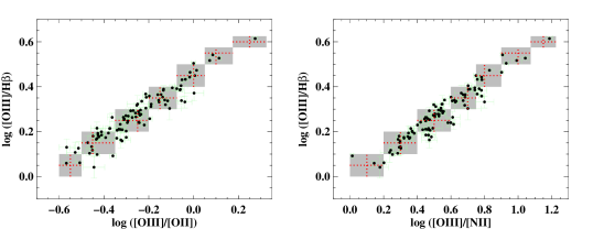
Figure 9: [O iii]/H$\beta$ line intensity ratio versus several intensity ratios sensitive to the ionization structure of the nebulae for the identified H ii regions in NGC 3310. Seven interval classes have been defined as the shaded regions in the different plots. All ratios for a given H ii region lies on the same class or in-between two classes. A typical average point value for each class is drawn as a red cross.

The main advantage in subtracting the stellar continuum is that the end product of such procedure is the percentage of each contributing stellar population to the light and mass. That is, we can estimate the mass of each stellar population responsible for the continuum emission. We may note, however, that any analysis technique has its own advantages and limitations. In particular, given the limited spectral range fitted (i.e. part of the optical), starlight gives a consistent description of the age of the ‘young’ population within 0.15-0.20 dex independently of the stellar templates used for an average age of $\tau\sim 100$ Myr (Cid Fernandes et al., 2013). Constraining the age of the population at $\tau\leq 10$Myr (expected for ionizing population) is highly uncertain using this technique alone. Therefore, including data from other spectral bands, especially at bluer wavelengths, helps to better constrain the properties of young ionizing populations.

Since this population is ionizing the gas, the emission lines we observe in the gas spectra give us useful information on its properties. For that reason, in the following we first compare the measured emission-line fluxes with those computed in photoionization models. This comparison gives us a first rough estimate of the age of the ionizing population and of the presence of dust grains. Next, we perform a multiwavelength analysis, covering a wider spectral range using SDSS and XMM-OM images. Finally, we combine both techniques to better constrain the age and the mass of the ionizing population.

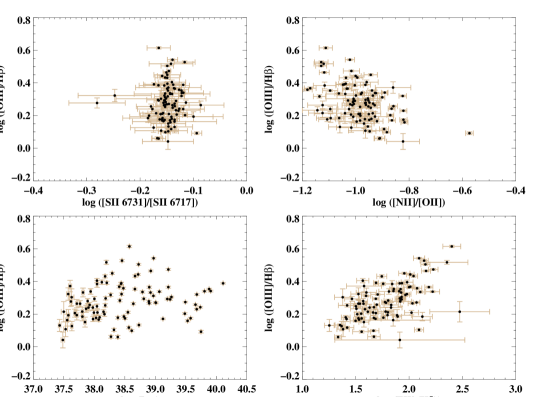
Figure 10: Same as in Fig. 9, but versus other sensitive intensity and intensity ratios. In this case no class has been defined since correlation are either weak (i.e. with [N ii]/[O ii], proxy to the abundance ratio N/O) or non-existent. The derived H$\beta$ luminosity is given in units of erg s^-1. The EW has been corrected by the continuum of the non-ionizing population.

3.4.1 Photoionization models

First of all, we took advantage of the knowledge of the ionization conditions of the gas within an H ii region. The strength of different line flux ratios depends on the shape of the ionizing continuum (i.e. age and metallicity of the young stellar population) and on the conditions and geometry of the cloud (i.e. electron density, temperature, clumpiness, absorption by dust grains, etc.). Based on this conception, we show in Figs. 9 and 10 the dependence of the [O iii]$\lambda$5007/H$\beta$ line intensity ratio (in log units) on other line ratios that provide information on the degree of ionization (e.g., the [O iii]/[O ii] ratio), the electron density of the cloud (ratios of the sulphur lines), the abundance, the electron temperature, the number of ionizing photons and the age of the burst (i.e. EW(H$\beta$ )).

As Fig. 9 illustrates, there is a good correlation between the [O iii]$\lambda$5007/H$\beta$ ratio and other line intensity ratios sensitive to the ionization structure of the cloud. We defined seven classes with different typical ratios (red dashed lines in the plot) and some width, which define the shaded areas, in such a way that in practically all cases the ratios for a given H ii region lies in the same class or in-between two classes. Class 1 would correspond to ratios on the bottom shaded area on the left with a typical log([O iii]/H$\beta$ ) ratio of 0.05. Moving right and up in the plot, the other classes are defined by the area of the shaded rectangles up to class seven where the typical log([O iii]/H$\beta$ ) ratio equals 0.6. On the other hand, as Fig. 10 shows, the ratio between the sulphur lines (sensitive to the electron density) and the H$\beta$ luminosities do not really depend on the [O iii]/[O ii] ratio. There is a mild dependence on the [N ii]/ oii ratio, sensitive to the abundance ratio N/O (Pérez-Montero & Díaz, 2005; Pérez-Montero & Contini, 2009) and on the EW(H$\beta$ ), which has been corrected for the contribution to the continuum by non-ionizing population as derived with starlight (see next section). Finally, although for classes 1–4 the logarithm of the H$\beta$ luminosity spans the whole range sampled (i.e. 37.5–40), for classes 5–7 the range is more restricted, from somewhat lower than 38.5 to somewhat higher than 39.0.

Table 3: cloudy simulations. Input line intensity ratio ranges, derived ages ($\tau$) and dust absorption factors ($f_{\mathrm{d}}$).

Class	Line ratio and EW ranges							Result of the fit
	[O ii]/H$\beta$	[O iii]/H$\beta$	[N ii]/H$\beta$	[S ii]1/H$\beta$	[S ii]2/H$\beta$	log L(H$\beta$ )	log EW (H$\beta$ )	log ($\tau$)	$f_{\mathrm{d}}$
						(erg s-1)	(Å)	(Myr)
1	3.16–5.00	1.00–1.26	0.63–1.26	0.63–1.26	0.53–0.84	37.5-38.5	1.35-1.65	6.71 ${}^{+0.02}_{-0.03}$	2.1 ${}^{+0.8}_{-0.4}$
						38.8-39.8		6.71 ${}^{+0.01}_{-0.03}$	2.3 ${}^{+0.6}_{-0.4}$
2	2.82–5.00	1.26–1.58	0.63–1.00	0.50–1.00	0.35–0.67	37.5-38.5	1.35-1.65	6.71 ${}^{+0.01}_{-0.03}$	2.4 ${}^{+0.9}_{-0.6}$
						38.8-39.8		6.71 ${}^{+0.02}_{-0.03}$	1.9 ${}^{+0.6}_{-0.4}$
3	2.50–4.47	1.58–2.00	0.50–0.80	0.47–0.79	0.28–0.56	37.5-38.5	1.6-2.1	6.65 ${}^{+0.02}_{-0.15}$	2.9 $\pm$ 1.2
						38.8-39.8		6.65 ${}^{+0.02}_{-0.05}$	3.0 ${}^{+1.3}_{-0.9}$
4	2.37–3.76	2.00–2.51	0.45–0.63	0.30–0.60	0.24–0.45	37.5-38.5	1.6-2.1	6.63 ${}^{+0.06}_{-0.04}$	1.3 ${}^{+0.4}_{-0.2}$
						38.8-39.8		6.64 ${}^{+0.03}_{-0.06}$	1.6 $\pm$ 0.4
5	2.24–3.76	2.51–3.16	0.32–0.56	0.28–0.47	0.21–0.38	38.5-39.5	1.6-2.1	6.63 ${}^{+0.04}_{-0.05}$	1.4 ${}^{+0.4}_{-0.3}$
6	2.11–3.35	3.16–3.76	0.32–0.47	0.27–0.42	0.21–0.32	38.5-39.5	2.05-2.35	6.58 ${}^{+0.03}_{-0.06}$	1.2 ${}^{+0.5}_{-0.1}$
7	1.99–2.82	3.76–4.22	0.22–0.35	0.22–0.35	0.13–0.24	38.5-39.5	2.05-2.35	6.55 ${}^{+0.06}_{-0.09}$	1.8 ${}^{+1.0}_{-0.6}$
Notes. [O iii]refers to [O iii]$\lambda$5007 Å, [N ii]to [N ii]$\lambda$6584 Å, [S ii]1 to [S ii]$\lambda$6717 Å and [S ii]2 to [S ii]$\lambda$6731 Å.

With this information, we have simulated the properties of the ionized gas and the stellar ionizing population for each class with the use of the photoionization code cloudy (version 10.0; Ferland et al. 1998). We took as ionizing sources the SEDs of ionizing star clusters spanning ages from 1 to 10 Myr using evolutionary synthesis techniques (popstar ; Mollá et al. 2009; Martín-Manjón et al. 2010). We used models with a Salpeter IMF, with masses between 0.15 and 100 M_⊙ . We assumed in all the models a radiation-bounded spherical geometry, a constant density of 100 particles cm^-3 and a standard fraction of dust grains in the interstellar medium (ISM). The presence of solid grains within the ionized gas can have some consequences on the physical conditions of the nebulae that should not be neglected. The heating of the dust can affect the equilibrium between the cooling and heating of the gas and, thus, the electron temperature inside the nebulae. The command PGRAINS, included in the last version of cloudy , implements the presence of dust grains as described in van Hoof et al. (2004). In all the models, the calculation was stopped when the temperature was lower than 4000 K. We also assumed that the gas has the same metallicity as the ionizing stars, covering the values 0.2Z_⊙ (0.008) and 0.4Z_⊙ (0.004) since gaseous abundances of H ii regions in this galaxy range typically between these two values (see Sect. 3.3.3). The other elemental abundances were set in solar proportions taking as a reference the phostosphere solar values given by Asplund et al. (2005), except in the case of nitrogen, for which we considered three different values of log(N/O), according to the mild correlation observed in Fig. 10: -1.05 (classes 6 and 7), -0.95 (classes 2–5) and -0.85 (class 1). We let the age of the ionizing population, the oxygen abundance, the number of ionizing photons, some geometrical parameters (inner radius and filling factor) and the content of dust grains vary in order to fit the line intensity ratios of oxygen, nitrogen and sulphur to H$\beta$ , together with the H$\beta$ luminosity and the continuum at 4885 Å (obtained with the EW(H$\beta$ )).

Once a compatible solution was found, we fixed all the fitted parameters save the dust grain content, the age of the ionizing population and the number of ionizing photons and run a grid of models varying these parameters. They are much more sensitive to line ratio variations, especially to the oxygen-to-H$\beta$ ratio. A solution in the grid was considered positive if it lied between the limits set by the shaded areas in Fig. 9. Note that any line ratio can be derived just by subtracting one value from the ‘y’-axis to that corresponding from the ‘x’-axis; for instance, log ([O iii]/H$\beta$ ) – log([O iii]/[N ii]) = log([N ii]/H$\beta$ ). A more constrained solution for each H ii region was obtained by comparing the observables derived with the model with the extinction corrected ratios, the H$\beta$ luminosity and the EW(H$\beta$ ) of each region.

Assumed intervals of the line intensity ratio for each class together with the solution for the ages are listed in Table 3. In general, the excitation can be explained in all cases by only one ionizing population of 3–5.5 Myr and, unlike starlight fitting, none around 1 Myr. Another important output from the grid of models corresponds to the UV absorption factor due to the internal extinction within the cloud, denoted as $f_{\mathrm{d}}$, also provided in the table. That is, if $f_{\mathrm{d}}$ = 1, no relevant absorption by dust grains is expected and if it is larger than 1, then such a factor is missed from the observed Balmer emission light. As inferred from the table, in all cases some emission is lost due to this UV absorption. In some cases, the loss is compatible with being marginal (i.e. for classes 4–6). However, in general, about 33% ($f_{\mathrm{d}}$ = 1.5) of the emitted UV photons or even more could be missed. Particularly, for class 3, the loss is expected to be quite high and up to more than a half of the emitted UV photons ($f_{\mathrm{d}}>$ 2.0) and even up to 75% ($f_{\mathrm{d}}\sim$ 4.0).

An individual model fit for each of the H ii region would be desirable. However, a few hundred iterations were needed in order to model only one class. This makes it a very long time consuming task. Nevertheless, we can complement the results obtained here with a spectrophotometric study by using a multiwavelength broad-band set of images and the spectral information provided by the Balmer emission lines. We develop this analysis in the following section.

3.4.2 Spectrophotometric analysis

XMM-OM and SDSS imaging can provide useful information on young stellar populations. In particular, having the information of ultraviolet and u broad-band emission makes a difference when trying to characterize ionizing stellar populations. The UV continuum is dominated by massive short-lived OB stars ($\tau\leq$ 100 Myr) and hence can be sensitive to star formation on time-scales of only 10 Myr or so. Likewise, as shown by Anders et al. (2004), u-band observations are essential for photometric investigations of young star clusters. Archive broad-band ultraviolet $UVW2$-$UVM2$ (OM) and u, i, z (SDSS) images were retrieved.

The main goal of our spectrophotometric study is to fit the SED of the young ionizing stellar population with models using the retrieved broad-band images and the spectral information provided by the IFU data. In particular, we gathered the data set as follows.

1. The five broad-band filter images just mentioned plus a set of three ‘simulated’ broad-band images, produced with the convolution of the IFS cubes with three known $HST$ filter throughput curves: $F439W\sim$ B Johnson, filter from the WFPC2 centred at 4300 Å; $F547M$, filter from the WFPC2 centred at 5479 Å; and $F621M$, filter from the WFC3 centred at 6219 Å. Fig. 11 shows the integrated spectrum of the galaxy with the throughput filter curves overplotted. Note that, thanks to the star–gas decoupling analysis we avoid contamination by the nebular emission lines on the continuum broad-band images (i.e. H$\gamma$ Balmer line just in the middle of the $F439W$ filter). Altogether, with our compiled multiwavelength data, we cover homogeneously a rather large spectral range (from the near-UV to the near-IR z band).

2. The H$\alpha$ and H$\beta$ line intensities and the respective EW, which set important constraints on the age of the ionizing stellar populations. The H$\alpha$ /H$\beta$ ratio is also directly related to the LOS extinction.

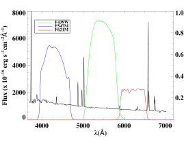
Figure 11: Convolved $HST$ filters with the IFS cubes.

With the aid of single stellar population models we can try to explain the observed photometric and spectroscopic properties of each H ii region in NGC 3310. However, we first have to take into account the non-ionizing stellar population. The results obtained with the starlight fitting are the key to decouple the light produced by ionizing and non-ionizing stellar populations. To that end we estimated, for each region and with the knowledge of the fitted stellar populations (i.e. starlight result), which fraction of the light at the effective wavelength of each photometric filter comes from the former or the latter. We used a conservative cut of 15 Myr to separate ionizing from non-ionizing populations. We could directly estimate this ratio with the stellar libraries used in starlight for the $HST$ filters, since the MILES library covers a wavelength range from 3525 to 7500 Å. To derive the other ratios the synthetic popstar templates were employed, since their spectral range covers all the filter data set used in this study and they include the nebular continuum contribution.

We remind the reader that we performed 100 starlight fits for each H ii region, which allowed us to estimate the uncertainties of these light ratios. In general, the light ratio for the bluest filters (i.e. UVW2,UVM2,u) is quite low, L_old/L$\mathrm{{}_{young}}\leq$ 2-10% (i.e. practically all the light is related to ionizing population). Even if the relative uncertainties can be high (up to 60%), they have little effect in the accuracy of the estimate of light related to young population. By contrast, the light ratio for red filters (i.e. i, z) can be easily larger than L_old/L$\mathrm{{}_{young}}=~{}$50% and up to 70%, with typical relative uncertainties of 20-30%.

In addition, by computing these ratios we are basically subtracting the contribution of the underlying old (in the sense of non-ionizing) stellar populations to the total emitted light. Therefore, we could correct the EWs of the H ii regions by subtracting this old population from the continuum. This corrected EW was used as an input parameter for the photoionization models in the previous section.

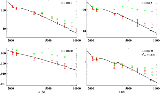
Figure 12: Synthetic best-fitting SED for four H ii regions. Photometric measurements corrected by non-ionizing population emission (not corrected) are overplotted in red (green). The correction is generally small (with some exception) for the ultraviolet data, while it is much more evident in redder filter photometric measurements. For the case where no solution is found, the value of $\chi^{2}_{\mathrm{min}}$ is labelled at the top right corner.

The following step was to perform the photometry of the H ii regions in NGC 3310. With the ‘simulated’ broad-band images with the $HST$ filters we directly added up all the flux contained in the spaxels that define the region. We want to use the same irregular aperture for all the images; hence, we preferred not to degrade all images to that with the worst one. Instead an IDL script was produced to add the flux of the same irregular aperture. Basically, all the images are re-sampled (preserving the flux) to have spaxels a factor of 10 smaller, so as to obtain a sub-spaxel photometry. The aperture is also re-sampled in such a way that the new aperture corresponds to the border of the previous one. Aperture coordinates are transformed to spaxel coordinates for each image and the flux within a given aperture is obtained adding up the flux of all the spaxels inside the aperture. Poisson noise is assumed, particularly important for the ultraviolet measurements, where only a few counts s^-1 are detected in many regions. To account for differential spatial resolution the aperture is also shifted by 1 arcsec in four directions (north, south, east and west), and median values and dispersions are taken to compute the final flux and error for each H ii region.

The response of the OM monitor at high count rates is not linear, an effect known as coincidence-loss  (Fordham et al., 2000). However, we have to corrected for this effect on our UV measurements because the count rates of the brightest H ii region on the individual exposures is of the order of 5 counts s^-1, below the critical rate of 10 counts s^-1 where this effect becomes significant (10%) according to the “XMM-Newton Users Handbook”, Issue 2.11, 2013 (ESA: XMM-Newton SOC). The count rate for the rest of the H ii regions is well below 5 counts s^-1, meaning that any systematic due to not correcting for this effect is well bellow 4%, much smaller than the typical uncertainties of the photometric measurements (see Table LABEL:table:result_chi_square).

Once the photometry was performed, the correction due to the underlying old population was applied. Altogether, at this stage we have the flux of the light related to the ionizing population through seven broad-band filters, the corrected EWs and the observed H$\alpha$ and H$\beta$ line fluxes. We have then compared observational and theoretical SEDs through a $\chi^{2}$-fitting procedure (Bik et al., 2003) as

$$\chi^{2}(Z,\tau,A_{V},m_{\star})=\sum_{N}\frac{(f_{\mathrm{obs}}-f_{\mathrm{model}})^{2}}{\sigma^{2}_{\mathrm{obs}}}$$ (8)

where $N$ denotes the number of filters and observables (photometric flux densities, fluxes and EWs of the emission lines; see Table LABEL:table:result_chi_square) available for each H ii region; $f_{\mathrm{obs}}$ and $f_{\mathrm{model}}$ are the observed and model observables, respectively; and $\sigma_{\mathrm{obs}}$ is the weight for the fit (i.e. photometric, line flux measurements and underlying population correction uncertainties). The $\chi^{2}$ minimization procedure for fitting SEDs produces more satisfactory results for determining the ages, extinctions, and masses in galaxies (e.g., Maoz et al. 2001; Bastian et al. 2005; Díaz-Santos et al. 2007) than other widely used methods such as colour–colour diagrams.

We first assumed that the stellar population responsible for the bulk of the ionization is a single stellar population for which four parameters were to be derived: metallicity ($Z$), age ($\tau$), extinction ($A_{V}$) and stellar mass ($m^{\mathrm{ion}}$). We used models with three different metallicities (0.2,0.4 and 1.0 Z_⊙). The expected (minimum) $\chi^{2}$ value of the best fit, $\chi^{2}_{\mathrm{min}}$, should be equal to the number of degrees of freedom ($\nu=N-4$). Those solutions within $\chi^{2}_{\mathrm{min}}\pm\Delta\chi^{2}_{\mathrm{min}}$, with $\Delta\chi^{2}_{\mathrm{min}}=(2\nu)^{\frac{1}{2}}$, were taken to determine the range of acceptable solutions. This would be equivalent to taking the $\pm 1\sigma$ solutions. Fig. 12 illustrates the results of the SED minimization fitting technique for different H ii regions in our sample: with high (ID 1, 3) and low (ID 86, 96) S/N spectra. The change of the shape of the spectra is quite evident when the correction due to underlying non-ionizing population is applied.

In Sect. 3.4.1 we explored the ionization structure of the seven classes, representative of the H ii regions. As a result we could estimate characteristic age and dust absorption factor ($f_{\mathrm{d}}$) intervals for each class. We have complemented those results with the SED fits presented here. In particular, we computed a grid of solutions of the $\chi^{2}$ minimization procedure by varying $f_{\mathrm{d}}$ from 1.0 to 4.5, that is, changing the modelled H$\alpha$ and H$\beta$ flux and the EWs, which are divided by $f_{\mathrm{d}}$ (when trying to recover the observed values some flux, scaled to $f_{\mathrm{d}}$, is lost). For a given H ii region, we then took those sets of solutions of the $\chi^{2}$ minimization procedure that were at the same time compatible with the age and $f_{\mathrm{d}}$ intervals in the class to which the region belongs. Some disagreement was encountered between the age interval derived from the $\chi^{2}$ fit and from the cloudy fit for a few H ii regions. However, the maximum difference is less than 1 Myr. For the vast majority of the regions the model that better reproduced the observables was that with $Z$ = 0.4Z_⊙, which is in agreement with the gaseous abundances derived in Sect. 3.3. Given the young nature of the ionizing population, this is expected.

The derived ages, stellar masses, internal extinctions and absorption factors are listed in Table LABEL:table:result_chi_square. The fit was not successful for a few cases, demanding the presence of two ionizing stellar populations. A minimization analysis was performed in those cases, though large degeneracy is found on the properties of the derived populations. One of them usually ranges between 1 and 6 Myr, the other being 6–15 Myr old. Within these age ranges the mass is not generally well defined within factors of less than 5–10.

We would like to mention that in a few cases no valid solutions were found for $f_{\mathrm{d}}=1$, but for $f_{\mathrm{d}}>1.0$. Thus, it may happen that the measured flux densities are related to a single stellar population but, since no solution is found, minimization techniques are immediately applied to a composite two-stellar-population model. As we have seen here, sometimes invoking a composite model is not necessary in order to reproduce the observed fluxes.

As can be observed in the table, H ii regions are typically 2.5–5 Myr old. This is consistent with the presence of WR stars (see the spectral features in Fig. 5), given that this phase normally starts 2–3 Myr after their birth (Meynet & Maeder, 2005). The mass of the ionizing stars span, on the other hand, a large range, from about $10^{4}$ up to 6$\times 10^{6}$ M_⊙ . Note the asymmetry on the error estimates. It is also worth mentioning the typical significant absorption factors derived ($f_{\mathrm{d}}$ = 1.3–3.0). According to our combined photoionization and spectrophotometric modelling, we have seen that, in general, at least 25% of the emitted UV photons from the OB stellar populations are absorbed by dust grains in the nebulae.

4 Discussion

4.1 Reliability on the stellar subtraction

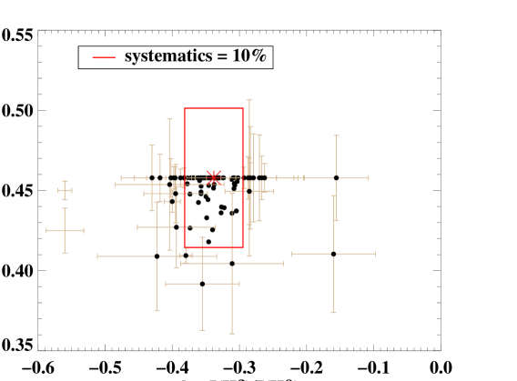
Figure 13: Balmer ratios with respect to H$\beta$ . The red asterisk marks the location on the plot of the theoretical ratio while the red box demarcates the ratio space where the values are within the expected systematics. To avoid confusion, typical error bars (median value) for H ii regions with ratios within the box are plotted on the left-hand side. The error is plotted for H ii regions with regions outside the plots.

In our analysis, we have been able to subtract the underlying continuum of the spectra and hence to decouple the gaseous and stellar contributions to the measured emission. For some parts of our analysis, this subtraction is critical. This is the case for the measurement of the [O iii]$\lambda$4363 Å line, since it is very close to H$\gamma$ , thus likely to be affected by a significant amount of underlying absorption. Here, we pay attention to the validity of such subtraction. We have hence checked the Balmer decrement ratios obtained once the extinction is corrected for each spectrum. Had we over-subtracted continuum absorption, negative extinction values and/or inconsistent Balmer ratios (i.e. H$\beta$ to H$\gamma$ ) would have been derived.

We present in Fig. 13 the derived Balmer ratios (or differences in logarithm units) and compare them with the theoretical values according to Osterbrock (1989) and assuming a case B recombination with $t_{\mathrm{e}}$ = 10,000 K and $n_{\mathrm{e}}$ = 100 cm^-3. Under these conditions, H$\alpha$ /H$\beta$ = 2.86 and H$\gamma$ /H$\beta$ = 0.459. Only four of them lie, within uncertainties, outside the systematic box. Although there are other 17 regions with ratios that lie outside the box, within uncertainties their ratios are consistent with the theoretical values. For those few cases where the ratio was not recovered because too much subtraction was performed, an extinction of $A_{V}=0$ mag was assigned.

4.2 Biases on temperature and abundance derivations

4.2.1 Methodologies used

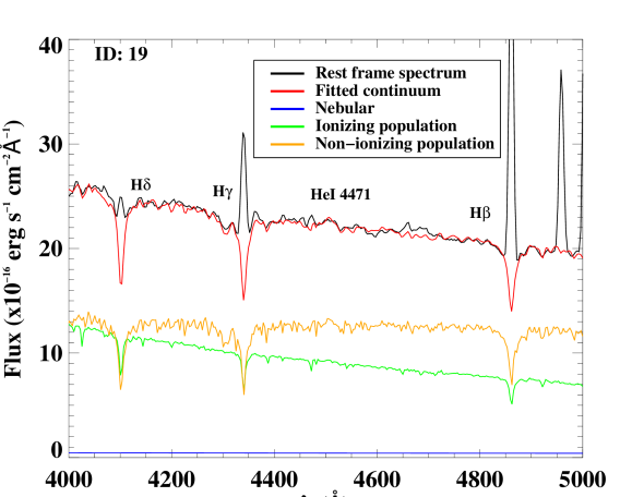
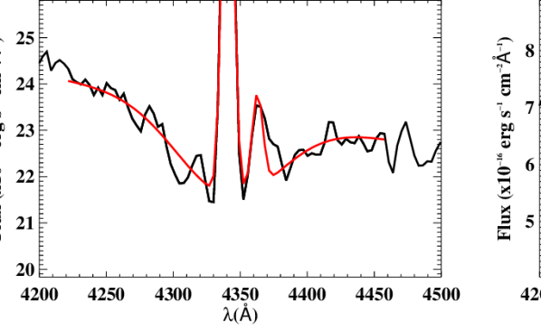
Figure 14: Left: rest-frame spectrum for H ii region ID 19 and the fitted components. See label for the identification of colours. The derived continuum spectrum is also plotted. Several Balmer lines (H$\beta$ ,H$\gamma$ ,H$\delta$ ) and the He i$\lambda$4771 Å line are also identified and labelled. Right: zoomed view centred on the H$\gamma$ spectral range. The red line shows the resulting fit of the two Gaussians (one for H$\gamma$ and the other for [O iii]$\lambda$4363 Å) and the negative Gaussian (for the absorption).

In Sect. 3.3.3 (Fig. 7) we show the abundance gradient in the disc of NGC 3310. An intrinsic dispersion of about 0.15 dex is observed along the disc for the $t_{\mathrm{e}}$-based derived oxygen abundances. They also show an offset of about 0.3 dex with respect to the abundances derived using strong-line calibrations.

In principle, it could be argued that abundances obtained through strong-line calibrations do suffer from typical systematics of 0.1–0.2 dex. However, we also have to keep in mind that accurate electron temperature determinations depend on reliable auroral line measurements, such as [S ii]$\lambda$6312 Å, [N ii]$\lambda$5755 Å or [O iii]$\lambda$4363 Å. The latter is very close to the H$\gamma$ line, which in young stellar populations can show a very wide profile (see Diaz 1988 for a detailed description of this complex spectral region). Given the spectral resolution of the PINGS data, the wings of both the oxygen auroral line and H$\gamma$ blend. In fact, as shown in Fig. 14 (left), the auroral line sets over the absorption wing of H$\gamma$ . A prominent stellar absorption can thus critically affect the measurement of the auroral line on the observed spectrum. Furthermore, the emission of this line is rather weak in regions with moderate abundance (12 + log(O/H) $\sim$ 8.0), and undetectable in metal-rich environments. Altogether, a reliable detection and measurement on this line can be rather awkward.

Very often, when fitting an emission line in a spectrum, a Gaussian function is assumed for the line and a straight line is used to fit the underlying continuum. For the specific case of [O iii]$\lambda$4363 Å, H$\gamma$ is also included as another Gaussian function in the fit due to its proximity. We have compared our $t_{\mathrm{e}}$ ([O iii]) ($\equiv t_{3}$) derivations with those that we would have obtained by fitting the auroral line directly on the ‘observed spectrum’, without the subtraction of the continuum obtained with starlight . Given that in most cases the stellar absorption is noticeable in the observed spectrum, instead of a straight line, the absorption was fitted with a broad Gaussian component with negative flux. An example of this is shown in Fig. 14 (right). Note that, as illustrated in the left-hand panel, part of the flux measured for the auroral line due to the fit actually corresponds to stellar continuum. The comparison of the electron temperature and the oxygen abundance using both methods is shown in Fig. 15 (left and middle). The electron temperature is usually overestimated, which causes a general underestimation of the metallicity if the measurements are done on the observed (unsubtracted) spectra. The difference between the derived temperatures (i.e. metallicities) is correlated with the ratio between the predicted absorption of H$\gamma$ with starlight and the corrected H$\gamma$ emission. It is hence directly related to the degree of absorption of the H$\gamma$ emission-line (see Fig. 15, right). By subtracting such absorption and fitting the residual spectra we obtain higher abundance values, in better agreement with the literature. Therefore, we do not think that the methodology applied to the measurement of the [O iii]$\lambda$4363 Å line flux is behind the significant difference found between the direct and strong-line abundance estimates.

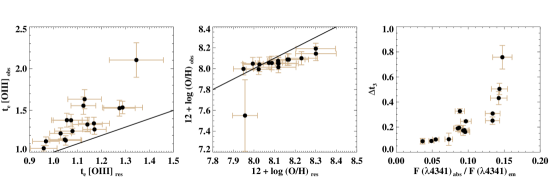
Figure 15: Left: comparison between the derived temperature $t_{3}$ using the observed and the residual spectra. Middle: comparison between the derived oxygen abundance using the observed and the residual spectra. In both cases the line represents the 1:1 relation. Right: comparison between the difference in electron temperatures ($\Delta t_{3}=t_{\mathrm{e}}\textrm{[{O\,{{iii}}}]}_{\textrm{obs}}-t_{\mathrm{e}}\textrm{[{O\,{{iii}}}]}_{\textrm{res}}$) and the flux ratio of H$\gamma$ in absorption to corrected H$\gamma$ in emission.

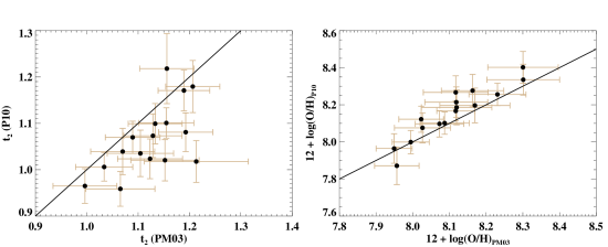
Figure 16: Left: comparison between the derived temperature $t_{2}$ using the $t_{2}$-$t_{3}$ relations provided by Pérez-Montero & Díaz (2003; PM03) and Pilyugin et al. (2010; P10). Right: relation between the derived oxygen abundance in each case. The line represents the 1:1 relation.

The use of different prescriptions used for the estimation of the $t_{\mathrm{e}}(\textrm{[{O\,{{ii}}}]})$ ($\equiv t_{2}$) may also contribute to the disagreement. As can be seen in Table 2, the ion O⁺ is generally more abundant than O²⁺. That is, the abundance determination is dominated in most cases by the knowledge of $t_{2}$. In most cases, our direct abundance determinations rely on our derived $t_{3}$. Therefore, using one or other parametrizations between both electron temperatures may change our abundance estimate to a significant extent.

There is not quite a consensus of how these temperatures are related. Several versions of the $t_{2}$-$t_{3}$ relation have been proposed, the most widely used by Campbell et al. (1986), based on the H ii region models of Stasińska (1982) is

$$t_{2}=0.7t_{3}+0.3$$ (9)

Several relations have been proposed during the last decades (e.g., Pagel et al. 1992; Izotov et al. 1997; Oey & Shields 2000; Pilyugin et al. 2006; Pilyugin & Thuan 2007). Here we focus on the relations proposed by Pérez-Montero & Díaz (2003; hereafter PM03) and Pilyugin et al. (2010; hereafter P10). In both cases, the physical conditions were derived using the five-level atom model for O⁺, O⁺⁺ and N⁺ ions, using the atomic data available. We compare these two works because the $ONS$ and $O3N2$ (O/N-corrected) calibrations were anchored to direct abundance determinations using a different $t_{2}$-$t_{3}$ relation. In particular, PM03 claim that this relation is density dependent (Eq. 2). On the other hand, P10 propose a relation quite similar to the commonly used ones (e.g., Campbell et al. 1986; Pagel et al. 1992):

$$t_{2}=0.672t_{3}+0.314$$ (10)

In Fig. 16, we compare the derived electron temperature $t_{2}$ (left) and oxygen abundance (right) using both sets of equations. In general, if we make use of the relations proposed in P10, the derived temperatures and abundances are systematically somewhat lower and higher, respectively. Given the uncertainties, the systematics on the abundance estimate are not important or relevant for at least half of the cases, especially for abundances $\sim 8.0$ or lower. However, in a few cases, abundances can be up to 0.1–0.2 dex higher, closer to the expected abundance values obtained with the strong-line calibrations. Therefore, the use of one set of equations or another can introduce systematics in abundance determinations of typically 0.1 dex.

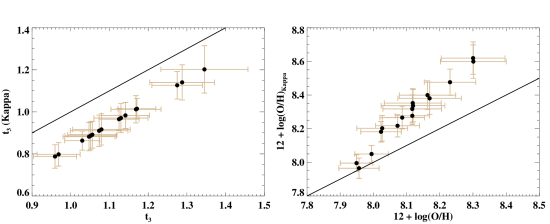
Figure 17: Left: comparison between the derived temperature $t_{3}$ using the conventional equilibrium methods (this study) and non-equilibrium methods (i.e. Kappa distribution). Right: relation between the derived oxygen abundance in each case. The line represents the 1:1 relation.

Even taking into account this offset, the discrepancy between direct and strong-line abundance estimates are still significant. The compilations used in order to obtain the strong-line calibrations consist of several hundreds of H ii regions. With such a high parameter space of ionization conditions to explore (age and mass of the ionizing population, ionization parameter, metallicity, N/O, density, etc.), it would not be surprising that the direct and strong-line abundance estimates of H ii regions with different ionizing conditions as those in the compilations differed. Larger compilations or models covering as much as possible the parameter space of ionization conditions would be needed.

4.2.2 The abundance discrepancy problem

Discrepancies on abundance determinations have been observed for decades. Chemical abundances determined from the optical recombination lines are systematically higher than those determined from CEL. This problem, dating back to 70 yr (Wyse 1942), was first discussed in detail by Torres-Peimbert & Peimbert (1977), and then regularly discussed in the literature (Liu et al. 2000; Stasińska 2004; Garcia-Rojas & Esteban 2006; García-Rojas & Esteban 2007; Stasińska et al. 2007; Mesa-Delgado et al. 2008). This is known as the ‘abundance discrepancy problem’. In addition, systematic differences between abundances determined using either direct measurements of ionic temperatures, or using SEL methods are reported in the literature (e.g., Kennicutt et al. 2003; Bresolin 2007; Bresolin et al. 2009; Ercolano et al. 2010; Pilyugin et al. 2012; López-Sánchez et al. 2012).

Unlike the systematics discussed in Sect. 4.2.1, most of the works just mentioned focus on the nature of the calibration used to define the strong-line method applied. In fact, there remains a significant offset (see Pérez-Montero et al. 2010; Dors et al. 2011) between those SEL techniques based purely upon photoionization models (McGaugh, 1991; Kewley & Dopita, 2002; Kobulnicky & Kewley, 2004) and those based upon an empirical alignment of the strong line intensities to abundances derived in objects for which the electron temperature has been directly estimated (Bresolin et al., 2004; Pilyugin & Thuan, 2005; Pilyugin et al., 2012). In some cases the abundance determinations via direct-temperature methods are favoured, (e.g. Bresolin et al. 2009; Ercolano et al. 2010) and the discrepancies are explained by the presence of multiple ionization sources (not taken into account in one-dimensional ionization models). In other cases, techniques based on photoionization models are preferred (e.g., Stasińska 2005; López-Sánchez et al. 2012), since they produce electron temperature gradients inside H ii regions, and temperature fluctuations are assumed to be the main reason for the abundance discrepancy problem.

Other physical scenarios have been proposed in order to explain this discrepancy, the most recent one exploring the fact that the electrons involved in collisional excitation and recombination processes may not be in thermal equilibrium (Binette et al. 2012; Nicholls et al. 2012, 2013). Here, we can estimate how would our direct abundance estimates be affected under this assumption. However, we cannot know how our estimates using strong-line methods are affected.

If we assume that the electrons involved in collisional excitation and recombination processes follow a non-equilibrium Kappa ($\kappa$) electron energy distribution rather than the widely assumed simple Maxwell–Boltzmann distribution, the ‘true’ electron temperature in the ionization zone is lower than the derived value using standard methods, as shown in Nicholls et al. (2013). They provide a means for estimating $\kappa$ with the knowledge of the “apparent” (i.e. derived using standard methods, like those used in this paper) [O iii] and [S iii] electron temperatures (see their fig. 11). Hägele et al. (2006) derived [O iii] and [S iii] electron temperatures in a large compilation of H ii galaxies and giant extragalactic H ii regions. A relation between both temperatures was found as

$$\mathrm{T([S{\sc III}])}=(1.19\pm 0.08)\times\mathrm{T([O{\sc III}])})-(0.32\pm 0.10)$$ (11)

Using this relation, we have made a rough estimation of $\kappa\sim 20$ within the range of temperatures in our study, in perfect agreement with the value obtained in Dopita et al. (2013). Nicholls et al. (2013) also provide a method to correct the electron temperature derived using standard methods, once $\kappa$ is known (see their Eq. 36). Although we are not able to compute the [S iii] electron temperature, we can estimate by how much a Kappa distribution with $\kappa\sim 20$ is affecting our temperature estimates, so as to speculate by up to how much our abundance determinations can be underestimated. As Fig. 17 shows, the electron temperatures might be overestimated by typically 2000 K, which translates into an underestimation (i.e. offset) of the oxygen abundance of typically 0.2 dex and up to 0.3 dex. This range agrees well with observed offsets (e.g. López-Sánchez et al. 2012). Note, however, that three regions still keep low-metallicity values (12 + log(O/H) $\sim$ 8.0) even if this correction is applied (Fig. 17, right).

4.3 Implications on the flat abundance gradient

The subject of abundance gradients in galaxies is currently a burning issue on galaxy evolution. The steepest abundance gradients were initially seen in late-type spiral galaxies (types Sb–Scd). Barred galaxies were thought to present shallower gradients  (Martin & Roy, 1994; Zaritsky et al., 1994), though more recent studies, with larger samples, have opened the debate that this may not be the case (Sánchez et al., 2012). Metallicity gradients can also be flattened or erased in interacting galaxies and remnants from mergers.

We have shown in Sect. 3.3.3 that the radial abundance gradient in NGC 3310 is rather flat. This is consistent with the flat gradients obtained in Sánchez et al. (2014) for merging galaxies at different levels of the interaction process. In a recent work, Werk et al. (2011) derived abundances for a handful of even more external H ii regions (up to a projected distance of almost 17 kpc or 6.7$r_{\mathrm{eff}}$ ). Although their abundance estimates are systematically higher than our estimates by about 0.2–0.3 dex (they use the model-based calibration of $R_{23}$), even at these distances they remain high and a flat abundance gradient is also observed. However, only a handful of H ii regions at a given azimuthal direction were observed in that study. We have observed over 100 regions and at all azimuthal directions. Therefore, combining both our and their study, we can be certain that the abundance gradient in NGC 3310 is rather flat from the very central regions to the outermost parts of the galaxy, well beyond 4$r_{\mathrm{eff}}$ .

This galaxy has been classified as a barred spiral. The bar and the size of the ringed structure suggest that this starburst was triggered by a bar instability (Piner et al., 1995). The likely past merger event this galaxy had with a dwarf plausibly produced the bar instability which led to the starburst. During an interaction, large amounts of gas can flow towards the central regions, carrying less enriched gas from the outskirts of the galaxy into the central regions, which can erase any metallicity gradient and dilute the central metallicity. Our results suggest that we are witnessing the consequences of such metal mixing processes.

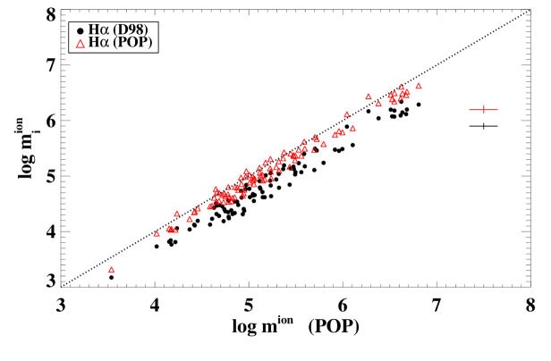
Figure 18: Comparison of the derived stellar ionizing mass using our spectrophotometric fitting (POP) with that derived using the extinction corrected H$\alpha$ flux plus the corrected (from underlying non-ionizing population) H$\beta$ EW width using Diaz’s (1998) and our updated prescription (H$\alpha$ D98 and H$\alpha$ POP, respectively). Typical errors are plotted at the top right corner. Whenever the H$\alpha$ flux and the EW(H$\beta$ ) are used, they are corrected for the derived absorption by dust grains. The dotted line indicates a unity relation.

Werk and collaborators measured flat radial oxygen abundance gradients from the central optical bodies to the outermost regions of the galaxies in their sample. Given the different morphology of the galaxies, star-forming properties and level of disruption (13 systems, not all of them with signs of interaction) in their sample, they argued that metal transport processes in cold neutral gas rather than interactions may also play an important role in distributing the metals to the outermost parts of the galaxies (e.g., magnetorotational instabilities, thermal instability triggered self-gravitational angular momentum transport, etc.). However, given the large time-scales required (i.e. 1.5 Gyr) and that the metals generated by massive stars are generally returned to the ISM in just $\sim$ 100 Myr (Tenorio-Tagle, 1996), they concluded that the metal transport may be occurring predominantly in a hot gas component, a still unclear driver mechanism. In any case, these other mechanisms do not exclude that interactions (even weak interactions or minor mergers) effectively mix the chemical metal content in a galaxy.

4.4 Star formation in NGC 3310

4.4.1 Different determinations of the mass of the ionizing population

In Sect. 3.4.2, we derive ages and masses for the ionized stellar population (i.e. with ages $\tau<10$ Myr). We can compare the stellar mass of the ionizing population as derived there and the values of the same masses derived from the extinction-corrected H$\alpha$ fluxes, using the expression from Díaz (1998):

$$\mathrm{log}~{}m^{\mathrm{ion}}=\mathrm{log}~{}L(\mathrm{H}\alpha)-0.86\times\mathrm{log}~{}\mathrm{EW(H}\beta)-32.61$$ (12)

This equation takes into account the evolutionary state of the ionizing stellar cluster, and the EW used corresponds to that that would be observed in the absence of an underlying population. As can be seen in Fig. 18 masses derived with the SED fitting are not consistent with those obtained from the H$\alpha$ flux. Actually, Eq. 12 is based basically on models by Garcia-Vargas et al. (1995a, b) and Stasińska & Leitherer (1996), all of them assuming a Salpeter IMF. We have updated this relation using popstar , the last version of these models. We have then explored the expected correlation between the number of ionizing photons per unit mass ($Q$(H)/M_⊙) and the EW of H$\beta$ , since both quantities decrease with the age of the cluster (see Fig. 19). A linear regression fit gives

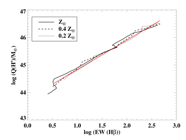
Figure 19: Relation between the number of ionizing photons per unit mass and the EW of H$\beta$ for different metallicities according to the popstar Single Stellar Population models (Mollá et al. 2009, Martín-Manjón et al. 2010). Red solid line represents the best fit for the model with $Z$ = 0.4Z$\odot$.

$$\mathrm{log}~{}Q(\mathrm{H})/\mathrm{M}_{\odot}=(1.07\pm 0.02)\times\mathrm{log}~{}\mathrm{EW}(\mathrm{H}\beta)+(43.76\pm 0.03)$$ (13)

for $Z$ = 0.4Z_⊙, and

$$\mathrm{log}~{}Q(\mathrm{H})/\mathrm{M}_{\odot}=(1.11\pm 0.03)\times\mathrm{log}~{}\mathrm{EW}(\mathrm{H}\beta)+(43.70\pm 0.05)$$ (14)

for $Z$ = Z_⊙

And the mass of the ionizing cluster, corrected by the evolutionary state is (for Z = 0.4Z_⊙):

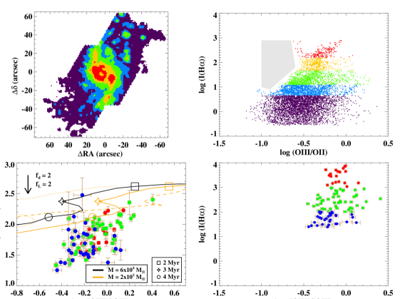
Figure 20: Top-left: H$\alpha$ intensity map, colour coded according to the intensity intervals defined on the right-hand (top-right) panel. Top-right: H$\alpha$ intensity (in log in arbitrary units) versus the excitation-sensitive ratio [O iii]/[O ii] for each spaxel. Different intensity intervals, log I(H$\alpha$ ), are colour coded as: $<$ 0.48 (violet), 0.48–0.90 (blue), 0.9–1.48 (green), 1.48–2.00 (orange), $>$ 2.00 (red). The grey area highlights the absence of low-excited and at the same time very luminous spaxels. Bottom-right: same relation as above, but for the H ii regions and different intensity intervals, log I(H$\alpha$ ), colour-coded as: $<$ 2.0 (blue), 2.0–3.0 (green), $>$ 4.0 (red). Bottom-left: EW(H$\beta$ ), only corrected by the presence of underlying non-ionizing population, versus excitation relation for the H ii regions, colour-coded according to the intensity intervals defined on the right-hand (bottom-left) panel. Superimposed tracks show the evolution of clusters of different initial mass with time along this relation, according to popstar models. Tracks in solid lines correspond to Z = 0.4Z_⊙, in dashed line to Z = 0.4Z_⊙ and in dotted line to Z = 0.2Z_⊙. The arrow at the upper-left corner illustrates by how much the tracks should be corrected if absorption by dust grains within the nebulae ($f_{\mathrm{d}}$) or escape ($f_{\mathrm{L}}$) of half of the ionizing photons occured.

$$\mathrm{log}~{}m^{\mathrm{ion}}=\mathrm{log}~{}L(\mathrm{H}\alpha)-1.07\times\mathrm{log}~{}\mathrm{EW(H}\beta)-31.90$$ (15)

If we use the new relation (for Z = 0.4Z_⊙, since the metallicity for the vast majority of H ii is around this value), then the derived mass is more similar to the adopted mass in this study (Fig. 18). Although within the uncertainties the mass are completely compatible, a small systematic offset of 0.1 dex is still present. Therefore, the mass obtained for the ionizing stellar population is little affected by the methodology used (SED $\chi^{2}$ minimization fitting or H$\alpha$ and EW of H$\beta$ with the updated relation).

It is interesting to mention that, if a fraction of photons escape or dust absorption of UV photons occur, both the H$\alpha$ flux and the EW measurements are affected in a similar way. Let us take $f_{\mathrm{Ld}}$ as the factor of photons that escape from the nebulae (leaking photons; ‘L’) and those are absorbed by dust grains (‘d’) within the nebulae. Since both the H$\alpha$ flux and the EW are shortened by the same factor, it is easy to work out the resulting relation for the mass of the ionizing stellar population (for $Z$ = 0.4Z_⊙):

$$\mathrm{log}~{}m^{\mathrm{ion}} \mspace{-20.0mu}=~{} \mathrm{log}~{}L(\mathrm{H}\alpha_{\mathrm{obs}})-1.07\times\mathrm{log}~{}\mathrm{EW(H}\beta_{\mathrm{obs}})~{}-\mspace{60.0mu}$$ (16)

$$-31.90-0.07\times\mathrm{log}~{}f_{Ld}$$

If $f_{\mathrm{Ld}}=2.0$, then the correction is just 0.02 dex. The typical range of $f_{\mathrm{d}}$ derived in this study (note that we have not estimated the fraction of leaking photons) is $f_{\mathrm{d}}=1.3-3.5$. Actually, even if two thirds of the photons are missing (i.e. $f_{\mathrm{d}}=3.0$), the correction would only amount 0.03 dex, which is lower than the typical uncertainty in the derivation of the mass.

4.4.2 Local evolutionary tracks

There is a clear correlation between the distance to the centre of the galaxy and the H$\alpha$ luminosity measured in NGC 3310, the circumnuclear whereabouts being the most luminous (see emission-line maps in Fig. 2). In order to explore if there is an evolutionary effect behind this relation we have investigated the conditions of the ionization in several H$\alpha$ luminosity intervals. As shown in Fig. 20 (top), the most luminous spaxels are generally also those with the hardest ionization. Even though there are a few spaxels with even higher degree of ionization, there is a clear envelope (lower part of grey area in the figure) at which no spaxel is very luminous and with low ionization. This cannot be a selection effect, because a spaxel with such conditions (being more luminous than average) should be observed. This effect, though less evident, is also observed when considering the H ii regions (Fig. 20, bottom-right).

The EW of H$\beta$ , once corrected by the continuum of non-ionizing populations, is a good indicator of the age of an ionizing cluster, i.e. of its evolutionary state (Dottori & Bica, 1981). A relation between the EW(H$\beta$ ) and the degree of ionization has been observed in H ii galaxies (Hoyos & Díaz, 2006). With our data we can reproduce a similar relation for the H ii regions of NGC 3310 (Fig. 20, bottom-left). Thus, this effect seems to be a local one, at least at the scale of one or a few hundred pc. According to the evolutionary tracks, the higher the initial mass of the ionizing population the harder the degree of ionization in the cloud for a fixed age. Note that these tracks are also metallicity dependent. At high metallicities, for a given age and mass of the ionizing population, the degree of ionization of the gas (i.e. [O iii]/[O ii]ratio) is lower and the EW just slightly smaller than at low metallicities. If, in general, the most luminous were more massive than the less luminous population, then the envelope we observe in the figure would be perfectly understandable. However, there is a general mismatch between observational data and models, quite evident in the figure. Given that the continuum from the underlying population has been subtracted, two reasons can be responsible for this disagreement, mainly: (i) absorption of UV photons by dust grains within the nebulae, which we have been able to roughly quantify in our analysis; (ii) escape of ionizing photons, which has been assumed to be negligible in this study. The arrow in Fig. 20 (bottom-left) exemplify by how much the tracks should be corrected by one or another. Additionally, the tracks shown in the figure only span a range up to 2$\times 10^{5}$ M_⊙ . Since the number of ionizing photons scales with the mass of the cluster, we would expect that by allowing a larger range in mass to the models the tracks would move towards harder ionizing regimes.

With the aid of the model tracks, we can speculate on the evolutionary state of the observed H ii regions. For instance, if the mass of the ionizing population is of the order of $10^{6}$ M_⊙  (the typical mass obtained for the most luminous ones, as reported in Table LABEL:table:result_chi_square) and assuming that the tracks move towards harder ionizing regimes at higher masses, then two possibilities can explain the observations: (i) the most luminous population is typically older than the less luminous ionizing population; (ii) the effect of dust absorption of UV photons and/or photon leakage can be important, which would explain at the same time why no H ii regions with high luminosity and low excitation are observed (i.e. log[O iii]/[O ii]$>$ 0.4).

4.4.3 Star Formation Rates

Although by definition, the star formation rate (SFR) of a starburst is zero when we see it several Myr later, with the knowledge of the mass and the age of the ionizing stellar population we can estimate an average SFR for each H ii region. The integrated value can give us a picture of the most recent star formation history of the galaxy (i.e. the rhythm at which the galaxy has been forming clusters during the last few Myr). We have made estimates of the SFR of the H ii regions just by computing the ratio of the mass and the age. Additionally, we have obtained another estimate by using the most widely used SFR rate calibrator in the optical, provided by Kennicutt (1998; K98). This calibrator relates the recent SFR with the H$\alpha$ luminosity as

$$\mathrm{SFR}(\mathrm{M}_{\odot}\mathrm{yr}^{-1})=7.49\times 10^{-42}~{}L\mathrm{(H}\alpha)~{}(\mathrm{ergs}^{-1})$$ (17)

The estimated SFRs using Kennicutt’s calibration are systematically lower than expected, even if we correct for absorption of dust grains (see Fig. 21). As cautioned in Kennicutt et al. (2007), the SFR derived using Eq. 17 for an individual H ii region, using a continuous star formation conversion relevant to entire galaxies, has limited physical meaning because the stars are younger and the region under examination is experiencing an instantaneous event when considered on any galactic evolutionary or dynamical time-scale.

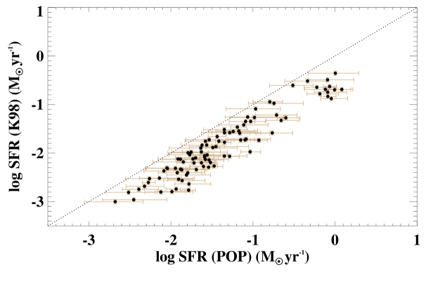
Figure 21: Comparison of the derived SFR using different methods our spectrophotometric fitting (POP) and the prescription by Kennicutt (1998; K98). Whenever the H$\alpha$ flux and the EW(H$\beta$ ) are used, they are corrected for the derived absorption by dust grains. The dotted line indicates a unity relation.

The integrated SFR using each method is 4.4 (Eq. 17) and 13.8 (spectrophotometric SED fitting), in units of M_⊙ yr^-1. These two estimates are in agreement with SFRs for starburst galaxies with moderate star formation (Kennicutt, 1998; Leitherer, 2000). Given our estimated age range ($\tau=$ 2.5 – 5 Myr) for the ionizing population, lower values using Kennicutt’s calibration are expected. Reported total SFR estimates are of the order of 3–8.6 M_⊙ yr^-1 (Smith et al., 1996; Werk et al., 2011; Mineo et al., 2012). They are within the range of (or somewhat below than) our estimates.

4.5 Mass growth in the disc of NGC 3310

In Sect. 3.4.2 we have shown that the ages of the ionizing population within the H ii regions span a very narrow range (i.e. $\tau=2.5-5.0$ Myr; see Table LABEL:table:result_chi_square). With such a narrow age range and a large H$\beta$ luminosity range (i.e. log H$\beta$ $\sim 1-3.5$; see Fig. 10), we can easily infer that there is not a correlation between the luminosity of an H ii region and the age of the ionizing population; that is, the most luminous H ii regions do not tend to be the youngest. Thus, we can assume that the luminosity of the H ii regions is roughly proportional to their masses, being their age a second-order effect.

Table 4: Comparison of mass derivations and ratios with those in H10.

HII	ID	mion	mion	m${}^{\mathrm{LOS}}_{\star}$	m${}^{dyn}_{\star}$	mion/m⋆	mion/m⋆
ID	H10		H10		H10	(%)	(%) H10
(1)	(2)	(3)	(4)	(5)	(6)	(7)	(8)
1+4	J	6.5${}^{+1.6}_{-1.5}$	1.29–3.14	220 $\pm$ 40	…	3.0${}^{+1.0}_{-0.8}$	…
3	N	6.7${}^{+1.1}_{-0.9}$	3.49	531${}^{+161}_{-82}$	74 $\pm$ 9	1.3 $\pm$ 0.3	4.7
5	R4	3.9${}^{+1.7}_{-1.1}$	1.76	177${}^{+106}_{-35}$	89 $\pm$ 3	2.1${}^{+1.0}_{-0.7}$	2.0
7	R5+R6+S6	3.2${}^{+1.4}_{-0.9}$	3.36	143${}^{+27}_{-14}$	103 $\pm$ 12	2.1${}^{+0.9}_{-0.6}$	3.3
8	R1+R2	1.9 $\pm$ 0.6	1.39	90${}^{+42}_{-21}$	91:	2.0${}^{+0.8}_{-0.6}$	1.5
11	R10+R11	4.4 $\pm$ 0.7	1.57	144${}^{+36}_{-6}$	59 $\pm$ 3	2.9 $\pm$ 0.5	2.7
12	R7	4.7${}^{+1.3}_{-1.1}$	0.87	157${}^{+31}_{-11}$	141 $\pm$ 6	2.8 $\pm$ 0.7	0.6
Notes. Col (1): H ii identification ID used in this study. Col (2): H ii identification ID of the individual or group of regions identified in H10, that correspond those identified in this study. Col (3): mass of the ionizing population derived in this study. Col (4): mass of the ionizing population derived in H10. Col (5): total stellar mass along the LOS derived in this study. Col (6): dynamical mass derived in H10. Col (7): ratio of the ionizing to the total stellar mass obtained in this study. Col (8): ratio of the ionizing to the total stellar mass (i.e. dynamical mass) obtained in H10. All masses are given in 106 M⊙ .

The contribution of the ionizing population to the total stellar population for each H ii region (i.e. the young to total stellar mass ratio, m^ion/m_⋆) can be roughly estimated by taking the derived mass of the starlight fitting as the total mass of the H ii region. Note that the total stellar mass actually represents the stellar mass along the LOS. Therefore, our estimation really represents a lower limit to the percentage. We would like to point out that the uncertainties on the derived total stellar masses (via the 100 realizations of the starlight fitting for each region) are generally strongly asymmetric. We thus took the $1\sigma$ uncertainties as the last values included within the 68% on the left ($\sigma^{-}$) and on the right ($\sigma^{-}$) of the mass distribution, centred on the median value. To better estimate the uncertainties on the m${}^{\mathrm{ion}}/$m_⋆ ratio we have used the techniques developed in Barlow (2003, 2004). In short, when an experimental result is represented as $x^{+\sigma^{+}}_{-\sigma^{-}}$, being $\sigma^{+}$ and $\sigma^{-}$ different, a non-symmetric distribution can represent $x$. Among the functions proposed in those papers, we modelled each variable (i.e. mass) using a “Variable Gaussian” parametrization. With an asymmetric distribution representing each variable we made a few tens of thousands of Monte Carlo runs for each H ii region using the idl routine ‘genrand’, which allows us to obtain random numbers following a given distribution (not necessarily normal) so as to obtain a reliable estimate of the mass ratio with its $\sigma^{+}$ and $\sigma^{-}$ uncertainty.

The derived m^ion/m_⋆ ratios range from 0.2 to about 7 per cent. A comparison for the circumnuclear regions in NGC 3310 identified in previous studies is shown in Table 4. Despite the fact that, with some exceptions, the ratios are similar, the disagreement between ionizing population and total stellar masses separately is evident, up to factors of more than 2 for the nucleus. Masses from the ionizing population reported in H10 were computed using Eq. 12. Apart from the systematic introduced by the use of the updated version presented in this study, aperture effects can contribute significantly to the differences in the reported H$\alpha$ luminosities and EW(H$\beta$ ), as Table 1 illustrates. In general, we have obtained higher mass values. In addition, we have generally computed higher total stellar masses because: (i) we have derived the LOS stellar mass; and (ii) H10 derived the total stellar mass of each cluster within an H ii region and then added up all the individual estimates for each region. In our calculations, the intracluster mass (probably from the disc) is included. Still, the ratios reported here and those obtained in H10 span a similar range, being always lower than 10%. All these values are also similar to those reported in H ii regions and H ii galaxies observed in other studies (Alonso-Herrero et al., 2001; Hägele et al., 2009; Pérez-Montero et al., 2010).

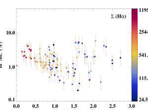
Figure 22: Radial distribution of the ratio between the stellar mass of the ionizing population and the total stellar mass along the LOS. The values are colour coded according to the H$\alpha$ surface density flux in 10^-16 erg s^-1 cm^-2 Å^-1 arcsec^-2. Only data for which an estimate of the ionizing mass via the SED fitting technique is plotted.

We show in Fig. 22 the radial distribution of this ratio (in terms of percentage) and its relation with the H$\alpha$ flux surface density. In general, those regions with higher H$\alpha$ flux surface density are located at smaller radii (with a few exceptions). The radial distribution of the young-to-total-stellar ratio is much more scattered. From the centre and up to about 1.5$r_{\mathrm{eff}}$  (where we cover the complete radial FoV), a 4.5$\sigma$ mild correlation is found, according to the Spearman’s rank-order correlation test. However, if we consider the whole radial range, such correlation cease to exist in statistical terms.

Given the narrow age range of the ionizing population we can roughly assume that any variation of the ratio between the ionizing population and the total stellar mass relates to a variation in the specific SFR (sSFR). In fact, if we compute the sSFR (just by subtracting the total mass from our estimates of the SFR) and plot it against the radial distance, we obtain a similar plot to that shown in Fig. 22. Therefore, just by examining this figure we can have some insight on the mass growth in the galaxy disc.

In the framework of the inside-out scenario, the SFR should be a strongly varying function of the galactocentric distance. Muñoz-Mateos et al. (2007) studied the radial profiles of sSFR for a sample of 161 nearby spiral galaxies. They found a large dispersion in the slope of these profiles with a slightly positive mean value, which they interpreted as proof of a moderate inside-out disc formation. Although they did not find any clear dependence of the sSFR gradient on the environment, they argued that transitory episodes of enhanced star formation in the inner parts of the disc can lead to a currently smaller SFR scalelength (gradual growth of the size of the disc with time) than in the past. That is, the gradient can hence be weakened or be even negative. It is well known that mergers in general can induce radial mixing processes, such as inflows of external gas on to the central regions and trigger starbursts (e.g., Barnes & Hernquist 1996; Rupke et al. 2010). As mentioned before, the global starburst in NGC 3310 is likely to have a minor merger origin (Smith et al., 1996; Kregel & Sancisi, 2001; Wehner et al., 2006). The mild negative gradient of the sSFR in NGC 3310 can well be another signature of a past merger event. This suggests that the minor merger event may be playing an important role in the mass build-up on the bulge, in agreement with recent models (Hopkins et al., 2010).

5 Conclusions

We have performed an IFS analysis in the distorted spiral galaxy NGC 3310, covering up to about 3 effective radii. This represents an unprecedented simultaneous spatial and spectroscopic coverage for this galaxy, which underwent a minor merger interaction some hundred Myr ago. While major mergers are known to cause dramatic changes in the progenitor galaxies, the impact of a minor merger is still not well understood. We have thus investigated on the evolution of the stellar and chemical properties of the galaxy on account of this past event. The paper relies on the analysis of the optical spectra of about a hundred H ii regions identified along the disc and spiral arms. Chemical abundances of the gas have been obtained by analysing the continuum-subtracted emission-line spectra, different techniques have been employed, and their radial distribution has been studied. We first fitted the SED of the galaxies using the program starlight in order to quantify the contribution of the underlying stellar population and perform such continuum subtraction. With the knowledge of the ionizing conditions of the H ii regions and the aid of ultraviolet and optical/NIR imaging we have characterized the properties (i.e. age, mass, SFR) of the ionizing population. The most important results of this study are summarized as follows.

1. All derived gaseous oxygen abundances using strong-line diagnostics, consistent with a sub-solar value (12 + log(O/H) $\sim$ 8.2–8.4), are similar to those reported for circumnuclear H ii regions present in this galaxy. With a sample of over 100 H ii regions we observe a rather flat abundance gradient in the disc of NGC 3310 out to about 10 kpc away from the nucleus. We can thus confirm the evidence that the minor merger event had a substantial impact on metal mixing in the remnant.

2. A direct ($t_{\mathrm{e}}$-based) oxygen abundance determination was possible in 16 H ii regions, located in the central regions of the galaxy. The derived values are somewhat lower and present more dispersion than those obtained using strong-line calibrations. With a statistically significant sample of H ii regions, we report on an offset of 0.2–0.3 dex between direct and strong-line abundance estimates. We argue several reasons behind the discrepancy: systematic uncertainties in the calibrations due to different ionization condition properties of the gas and different prescriptions used to relate electron temperatures between the ionic species. We further investigate the effect of the oversimplified assumption that the electrons in the nebulae are in thermal equilibrium on the determination of the direct abundances. Under the assumption of a non-equilibrium Kappa electron energy distribution, the adopted abundances would be increased by up to 0.2–0.3 dex.

3. With the use of single stellar population and photoionization models, we have been able to constrain the main properties of the ionizing stellar population within the H ii regions. In general, the presence of a single population is sufficient to explain the measured broad-band (from ultraviolet to $z$ band) and ionizing line-flux. The age of the ionizing population spans a narrow range of 2.5–5 Myr, whereas the mass range is quite large, from about 10⁴ to 6$\times 10^{6}$ M_⊙ . Given the ionized gas line ratios, dust grains must be present in most of the H ii regions, causing the absorption from a few percent and up to more than two-thirds (typical absorption factors of $f_{\mathrm{d}}=$1.3-3.5) of the UV photons.

4. We have updated prescriptions to derive the stellar mass of the ionizing population, correcting by its evolutionary state, with the knowledge of the H$\alpha$ flux and the EW of H$\beta$ . The ionizing mass has little dependence on photon losses by either UV photon leakage or absorption of UV photons by dust grains within the nebulae. The typical uncertainties of the derived masses, generally within a factor of 1.5–2, are in fact much higher than any correction that should be applied were these losses even of the order of 66%.

5. The derived average global SFR over time-scales $>$ 6 Myr, 4.4 M_⊙ yr^-1, is consistent with other studies made at other wavelengths. However, the average global SFR for the last few Myr (i.e. $\lesssim$ 5 Myr) is about a factor of 3 higher.

6. The mass of the ionizing population represents generally less than 5% of the estimated population along the LOS, down to about 0.2%. Taking into account that the contribution of the old mass of the disc is not subtracted, this result is consistent with other studies that support that in circumnuclear regions the ratio of the ionizing to total stellar mass is typically of the order of a few percent, less than 10%. The radial distribution of the specific SFR (proportional to this ratio) in the disc of NGC 3310 suggests that minor interactions indeed can play an important role in the formation and assembly of the bulge.

Appendix A Catalogue tables

Table 5: Catalogue of H ii regions and reddeing corrected derived line intensities

H ii ID	$\Delta$ AR	$\Delta\delta$	$r_{\mathrm{d}}$	[O ii] 3727,3729	H$\gamma$	H$\beta$	[O iii] 4959	[O iii] 5007	[N ii] 6548	H$\alpha$	[N ii] 6584	[S ii] 6717	[S ii] 6731	log I(H$\beta$)	c (H$\beta$)
(1)	(2–4)			(5–14)										(15)	(16)
1	9.09	-4.86	11.88	280.2 $\pm$ 5.1	44.7 $\pm$ 0.5	100.0 $\pm$ 0.5	81.3 $\pm$ 1.7	244.5 $\pm$ 2.6	16.7 $\pm$ 0.2	287.0 $\pm$ 2.9	48.3 $\pm$ 1.7	31.2 $\pm$ 0.3	23.7 $\pm$ 0.2	-12.38	0.13 $\pm$ 0.03
2	-7.08	0.27	8.92	294.8 $\pm$ 6.0	44.4 $\pm$ 0.4	100.0 $\pm$ 0.4	72.4 $\pm$ 2.0	219.2 $\pm$ 2.8	20.7 $\pm$ 0.2	287.0 $\pm$ 2.1	60.0 $\pm$ 1.0	37.9 $\pm$ 0.3	28.7 $\pm$ 0.2	-12.58	0.16 $\pm$ 0.03
3	0.00	0.00	0.00	283.1 $\pm$ 9.9	50.9 $\pm$ 1.5	100.0 $\pm$ 0.9	39.6 $\pm$ 1.1	123.6 $\pm$ 2.3	41.4 $\pm$ 0.7	287.0 $\pm$ 4.4	119.8 $\pm$ 1.9	48.7 $\pm$ 0.9	39.2 $\pm$ 0.8	-12.74	0.14 $\pm$ 0.03
4	7.91	-9.67	13.07	313.1 $\pm$ 6.6	46.6 $\pm$ 0.5	100.0 $\pm$ 0.6	71.9 $\pm$ 1.6	218.7 $\pm$ 2.5	18.1 $\pm$ 0.2	287.0 $\pm$ 2.9	52.3 $\pm$ 1.5	38.9 $\pm$ 0.3	29.6 $\pm$ 0.3	-12.68	0.07 $\pm$ 0.03
5	-4.71	3.69	6.60	279.0 $\pm$ 7.0	46.5 $\pm$ 0.5	100.0 $\pm$ 0.6	67.2 $\pm$ 1.7	208.9 $\pm$ 2.5	22.9 $\pm$ 0.3	287.0 $\pm$ 2.5	66.3 $\pm$ 1.2	37.1 $\pm$ 0.4	28.0 $\pm$ 0.4	-12.81	0.08 $\pm$ 0.03
6	-5.85	-6.50	10.64	281.5 $\pm$ 6.6	45.0 $\pm$ 0.6	100.0 $\pm$ 0.5	55.9 $\pm$ 1.4	169.6 $\pm$ 2.0	23.2 $\pm$ 0.3	287.0 $\pm$ 2.2	67.4 $\pm$ 1.1	45.2 $\pm$ 0.4	33.7 $\pm$ 0.3	-12.81	0.05 $\pm$ 0.03
7	-2.81	7.00	7.56	284.1 $\pm$ 6.8	47.4 $\pm$ 0.5	100.0 $\pm$ 0.5	59.1 $\pm$ 1.4	181.0 $\pm$ 2.0	21.5 $\pm$ 0.2	287.0 $\pm$ 2.4	62.4 $\pm$ 1.2	40.4 $\pm$ 0.3	29.6 $\pm$ 0.3	-12.83	0.09 $\pm$ 0.03
8	-10.52	4.11	13.38	310.0 $\pm$ 8.0	46.1 $\pm$ 0.6	100.0 $\pm$ 0.5	73.7 $\pm$ 1.7	225.7 $\pm$ 2.5	19.6 $\pm$ 0.2	287.0 $\pm$ 2.2	56.6 $\pm$ 1.1	40.2 $\pm$ 0.4	30.3 $\pm$ 0.3	-12.61	0.28 $\pm$ 0.02
9	-9.57	-4.19	13.41	307.2 $\pm$ 6.8	46.6 $\pm$ 0.6	100.0 $\pm$ 0.5	58.5 $\pm$ 1.4	174.6 $\pm$ 2.0	22.9 $\pm$ 0.3	287.0 $\pm$ 2.2	66.4 $\pm$ 1.1	48.2 $\pm$ 0.4	36.0 $\pm$ 0.3	-12.75	0.14 $\pm$ 0.03
10	-1.80	-8.98	9.82	318.6 $\pm$ 7.2	48.8 $\pm$ 0.8	100.0 $\pm$ 0.5	51.7 $\pm$ 1.5	159.4 $\pm$ 2.1	23.5 $\pm$ 0.3	286.4 $\pm$ 2.3	68.1 $\pm$ 1.2	44.1 $\pm$ 0.4	33.8 $\pm$ 0.4	-13.01	0.00 $\pm$ 0.03
11	0.30	-5.04	5.14	298.6 $\pm$ 7.3	49.1 $\pm$ 0.9	100.0 $\pm$ 0.6	46.4 $\pm$ 1.4	149.5 $\pm$ 2.1	24.6 $\pm$ 0.4	287.0 $\pm$ 2.8	71.4 $\pm$ 1.4	47.5 $\pm$ 0.6	34.8 $\pm$ 0.5	-12.91	0.05 $\pm$ 0.03
12	3.08	5.71	7.49	300.3 $\pm$ 7.5	45.9 $\pm$ 0.9	100.0 $\pm$ 0.6	46.0 $\pm$ 1.5	144.0 $\pm$ 2.1	25.0 $\pm$ 0.4	282.8 $\pm$ 2.5	72.5 $\pm$ 1.2	52.1 $\pm$ 0.6	37.5 $\pm$ 0.5	-12.96	0.00 $\pm$ 0.01
13	-11.09	10.50	16.44	325.7 $\pm$ 6.6	44.0 $\pm$ 0.5	100.0 $\pm$ 0.4	63.0 $\pm$ 1.3	187.6 $\pm$ 1.9	20.7 $\pm$ 0.2	287.0 $\pm$ 2.1	60.0 $\pm$ 1.0	49.0 $\pm$ 0.4	35.9 $\pm$ 0.4	-13.00	0.15 $\pm$ 0.03
14	5.57	-27.60	28.24	288.2 $\pm$ 6.1	42.7 $\pm$ 0.6	100.0 $\pm$ 0.5	107.0 $\pm$ 2.8	297.3 $\pm$ 3.9	15.2 $\pm$ 0.2	287.0 $\pm$ 4.0	44.0 $\pm$ 2.6	34.8 $\pm$ 0.3	24.9 $\pm$ 0.2	-13.28	0.18 $\pm$ 0.03
15	-8.89	14.96	17.72	329.4 $\pm$ 7.0	46.8 $\pm$ 0.5	100.0 $\pm$ 0.4	68.8 $\pm$ 1.7	201.8 $\pm$ 2.3	20.0 $\pm$ 0.2	287.0 $\pm$ 2.8	58.0 $\pm$ 1.8	51.5 $\pm$ 0.4	36.4 $\pm$ 0.3	-13.23	0.05 $\pm$ 0.03
16	-9.56	19.54	21.93	343.6 $\pm$ 7.0	44.6 $\pm$ 0.6	100.0 $\pm$ 0.5	64.5 $\pm$ 1.7	195.0 $\pm$ 2.5	18.7 $\pm$ 0.2	287.0 $\pm$ 2.5	54.1 $\pm$ 1.2	47.8 $\pm$ 0.4	35.3 $\pm$ 0.4	-13.25	0.10 $\pm$ 0.03
17	1.73	-29.36	29.94	323.7 $\pm$ 5.3	45.5 $\pm$ 0.5	100.0 $\pm$ 0.5	80.8 $\pm$ 2.3	231.7 $\pm$ 3.2	16.5 $\pm$ 0.2	287.0 $\pm$ 2.9	47.8 $\pm$ 1.6	41.9 $\pm$ 0.5	29.7 $\pm$ 0.4	-13.28	0.26 $\pm$ 0.02
18	1.56	-24.46	24.94	283.7 $\pm$ 5.3	42.7 $\pm$ 0.6	100.0 $\pm$ 0.6	73.5 $\pm$ 1.6	217.4 $\pm$ 2.5	18.5 $\pm$ 0.3	287.0 $\pm$ 3.8	53.6 $\pm$ 2.4	48.7 $\pm$ 0.5	35.0 $\pm$ 0.4	-13.43	0.19 $\pm$ 0.03
19	-3.91	11.98	12.60	326.3 $\pm$ 8.1	44.1 $\pm$ 0.7	100.0 $\pm$ 0.5	48.5 $\pm$ 1.2	148.2 $\pm$ 1.7	24.4 $\pm$ 0.3	287.0 $\pm$ 2.5	70.7 $\pm$ 1.1	60.7 $\pm$ 0.8	43.6 $\pm$ 0.7	-13.37	0.03 $\pm$ 0.03
20	-5.36	21.84	22.51	329.1 $\pm$ 8.4	43.5 $\pm$ 0.7	100.0 $\pm$ 0.7	66.8 $\pm$ 1.8	189.8 $\pm$ 2.6	19.6 $\pm$ 0.4	277.0 $\pm$ 2.8	56.9 $\pm$ 1.3	55.3 $\pm$ 0.6	38.6 $\pm$ 0.5	-13.60	0.00
21	-9.65	25.08	26.92	363.5 $\pm$ 8.3	42.8 $\pm$ 0.6	100.0 $\pm$ 0.7	61.8 $\pm$ 1.9	185.8 $\pm$ 2.8	19.0 $\pm$ 0.4	287.0 $\pm$ 2.9	55.0 $\pm$ 1.3	55.4 $\pm$ 0.6	39.3 $\pm$ 0.5	-13.48	0.12 $\pm$ 0.03
22	-5.67	-34.75	37.40	302.0 $\pm$ 8.2	43.9 $\pm$ 0.7	100.0 $\pm$ 0.6	96.3 $\pm$ 2.3	291.2 $\pm$ 3.6	12.6 $\pm$ 0.3	287.0 $\pm$ 2.7	36.5 $\pm$ 1.0	36.4 $\pm$ 0.4	25.7 $\pm$ 0.4	-13.57	0.10 $\pm$ 0.03
23	7.33	-23.08	24.22	333.6 $\pm$ 7.8	40.9 $\pm$ 0.7	100.0 $\pm$ 0.6	67.1 $\pm$ 1.4	184.4 $\pm$ 2.2	19.9 $\pm$ 0.4	287.0 $\pm$ 3.6	57.7 $\pm$ 2.1	51.8 $\pm$ 0.6	36.4 $\pm$ 0.5	-13.59	0.08 $\pm$ 0.03
24	7.00	-18.00	19.35	373.9 $\pm$ 7.2	44.2 $\pm$ 0.8	100.0 $\pm$ 0.7	63.2 $\pm$ 1.6	196.0 $\pm$ 2.5	19.2 $\pm$ 0.3	287.0 $\pm$ 3.5	55.5 $\pm$ 1.9	54.3 $\pm$ 0.5	37.1 $\pm$ 0.4	-13.29	0.19 $\pm$ 0.03
25	25.00	15.74	37.49	374.2 $\pm$ 6.3	46.0 $\pm$ 0.6	100.0 $\pm$ 0.5	62.3 $\pm$ 1.0	186.7 $\pm$ 1.7	20.2 $\pm$ 0.3	287.0 $\pm$ 3.0	58.4 $\pm$ 1.7	41.9 $\pm$ 0.5	30.0 $\pm$ 0.4	-13.49	0.13 $\pm$ 0.03
26	5.18	24.91	27.30	306.0 $\pm$ 6.7	43.9 $\pm$ 0.6	100.0 $\pm$ 0.6	71.5 $\pm$ 1.4	214.8 $\pm$ 2.3	17.5 $\pm$ 0.3	287.0 $\pm$ 2.6	50.7 $\pm$ 1.1	42.5 $\pm$ 0.5	30.6 $\pm$ 0.4	-13.57	0.10 $\pm$ 0.03
27	23.00	41.74	55.12	286.0 $\pm$ 6.2	46.1 $\pm$ 0.8	100.0 $\pm$ 0.6	119.3 $\pm$ 2.5	348.3 $\pm$ 3.8	14.9 $\pm$ 0.4	287.0 $\pm$ 2.8	43.1 $\pm$ 1.3	33.7 $\pm$ 0.5	24.4 $\pm$ 0.4	-13.52	0.12 $\pm$ 0.03
28	-16.00	-4.26	21.30	317.4 $\pm$ 6.0	45.1 $\pm$ 0.9	100.0 $\pm$ 0.6	66.8 $\pm$ 1.5	204.9 $\pm$ 2.5	21.8 $\pm$ 0.5	283.9 $\pm$ 2.5	63.3 $\pm$ 1.0	56.9 $\pm$ 0.7	40.0 $\pm$ 0.6	-13.52	0.00 $\pm$ 0.02
29	2.26	-33.66	34.30	334.5 $\pm$ 7.0	42.9 $\pm$ 0.9	100.0 $\pm$ 0.8	75.4 $\pm$ 2.3	231.6 $\pm$ 3.6	17.0 $\pm$ 0.5	287.0 $\pm$ 3.6	49.1 $\pm$ 1.6	45.7 $\pm$ 0.7	33.5 $\pm$ 0.6	-13.59	0.21 $\pm$ 0.03
30	8.19	-33.15	34.18	294.7 $\pm$ 9.7	39.8 $\pm$ 1.1	100.0 $\pm$ 1.0	95.5 $\pm$ 2.6	271.0 $\pm$ 4.5	16.3 $\pm$ 0.5	277.4 $\pm$ 4.3	47.4 $\pm$ 1.7	41.1 $\pm$ 0.8	28.9 $\pm$ 0.7	-13.82	0.00
31	-2.52	-31.02	32.49	368.8 $\pm$ 7.6	49.0 $\pm$ 1.0	100.0 $\pm$ 0.8	71.5 $\pm$ 2.1	216.4 $\pm$ 3.3	17.5 $\pm$ 0.5	287.0 $\pm$ 3.4	50.5 $\pm$ 1.4	50.5 $\pm$ 0.7	35.5 $\pm$ 0.6	-13.70	0.20 $\pm$ 0.03
32	10.41	-28.82	30.67	288.6 $\pm$ 7.5	42.3 $\pm$ 0.7	100.0 $\pm$ 0.6	102.1 $\pm$ 2.5	277.2 $\pm$ 3.6	15.8 $\pm$ 0.4	267.0 $\pm$ 3.1	45.7 $\pm$ 1.6	39.9 $\pm$ 0.6	27.7 $\pm$ 0.5	-13.77	0.00
33	42.00	37.74	70.05	218.7 $\pm$ 6.8	46.0 $\pm$ 1.2	100.0 $\pm$ 1.0	147.0 $\pm$ 3.7	411.6 $\pm$ 6.3	9.2 $\pm$ 0.6	284.3 $\pm$ 4.4	26.8 $\pm$ 1.2	28.7 $\pm$ 0.9	19.6 $\pm$ 0.8	-13.92	0.00 $\pm$ 0.02
34	24.00	22.74	40.83	319.4 $\pm$ 8.5	49.1 $\pm$ 1.1	100.0 $\pm$ 0.9	106.8 $\pm$ 2.0	319.4 $\pm$ 4.0	13.0 $\pm$ 0.5	287.0 $\pm$ 3.8	37.6 $\pm$ 1.4	36.5 $\pm$ 0.7	25.9 $\pm$ 0.6	-13.77	0.07 $\pm$ 0.03
35	17.00	-11.26	22.94	365.6 $\pm$ 11.3	41.7 $\pm$ 0.9	100.0 $\pm$ 0.7	69.7 $\pm$ 1.7	196.7 $\pm$ 2.7	19.6 $\pm$ 0.5	256.7 $\pm$ 2.8	56.9 $\pm$ 1.3	57.1 $\pm$ 0.8	40.1 $\pm$ 0.7	-13.68	0.00
36	17.00	-0.26	21.46	387.0 $\pm$ 11.5	49.2 $\pm$ 1.1	100.0 $\pm$ 0.8	44.9 $\pm$ 1.1	135.8 $\pm$ 1.8	23.5 $\pm$ 0.6	282.6 $\pm$ 3.2	68.1 $\pm$ 1.4	66.7 $\pm$ 0.9	47.5 $\pm$ 0.8	-13.76	0.00 $\pm$ 0.01
37	-5.86	27.74	28.42	350.1 $\pm$ 13.3	41.5 $\pm$ 1.1	100.0 $\pm$ 0.9	53.1 $\pm$ 1.5	162.5 $\pm$ 2.6	19.9 $\pm$ 0.7	287.0 $\pm$ 4.2	57.6 $\pm$ 1.9	62.6 $\pm$ 1.1	43.5 $\pm$ 0.9	-13.94	0.01 $\pm$ 0.03
38	18.05	63.44	72.05	259.2 $\pm$ 6.3	46.2 $\pm$ 1.1	100.0 $\pm$ 0.9	112.4 $\pm$ 3.4	336.8 $\pm$ 5.5	10.5 $\pm$ 0.6	287.0 $\pm$ 4.4	30.5 $\pm$ 1.6	28.4 $\pm$ 0.8	21.7 $\pm$ 0.7	-14.04	0.02 $\pm$ 0.03
39	-2.96	-38.65	40.42	366.7 $\pm$ 16.0	45.5 $\pm$ 1.3	100.0 $\pm$ 1.0	72.9 $\pm$ 1.7	225.4 $\pm$ 3.3	16.1 $\pm$ 0.7	287.0 $\pm$ 4.6	46.6 $\pm$ 2.0	45.8 $\pm$ 1.0	32.6 $\pm$ 0.9	-13.83	0.14 $\pm$ 0.03
40	1.82	20.56	21.57	337.7 $\pm$ 8.9	45.1 $\pm$ 1.0	100.0 $\pm$ 0.8	41.2 $\pm$ 1.1	125.3 $\pm$ 1.8	24.2 $\pm$ 0.7	287.0 $\pm$ 3.2	70.1 $\pm$ 1.5	70.2 $\pm$ 1.2	49.4 $\pm$ 1.0	-13.88	0.01 $\pm$ 0.03
41	-19.00	8.74	24.44	344.3 $\pm$ 11.3	46.0 $\pm$ 1.2	100.0 $\pm$ 0.8	60.8 $\pm$ 1.8	183.3 $\pm$ 2.8	22.2 $\pm$ 0.8	287.0 $\pm$ 3.9	64.3 $\pm$ 2.0	59.9 $\pm$ 1.2	41.9 $\pm$ 1.1	-13.85	0.03 $\pm$ 0.03
42	-9.50	-37.53	41.98	279.3 $\pm$ 12.5	43.5 $\pm$ 1.4	100.0 $\pm$ 1.1	79.1 $\pm$ 2.2	243.0 $\pm$ 4.8	15.2 $\pm$ 1.3	287.0 $\pm$ 5.2	43.9 $\pm$ 2.2	42.7 $\pm$ 1.5	29.2 $\pm$ 1.3	-14.05	0.02 $\pm$ 0.03
43	-10.79	-24.36	30.15	324.6 $\pm$ 10.1	44.7 $\pm$ 1.2	100.0 $\pm$ 0.8	70.2 $\pm$ 2.2	210.1 $\pm$ 3.5	20.6 $\pm$ 0.7	279.4 $\pm$ 3.4	59.7 $\pm$ 1.5	59.2 $\pm$ 1.0	41.5 $\pm$ 0.8	-14.05	0.00
44	-21.30	-14.17	32.39	368.1 $\pm$ 10.6	46.7 $\pm$ 1.2	100.0 $\pm$ 0.9	48.5 $\pm$ 1.1	149.1 $\pm$ 2.0	22.6 $\pm$ 0.6	287.0 $\pm$ 3.6	65.6 $\pm$ 1.6	60.6 $\pm$ 1.1	42.5 $\pm$ 0.9	-13.99	0.07 $\pm$ 0.03
45	6.18	42.56	45.50	333.5 $\pm$ 11.7	40.2 $\pm$ 1.3	100.0 $\pm$ 0.9	82.7 $\pm$ 2.1	245.0 $\pm$ 3.6	16.3 $\pm$ 0.9	287.0 $\pm$ 4.5	47.4 $\pm$ 2.0	49.3 $\pm$ 1.2	35.9 $\pm$ 1.0	-14.05	0.01 $\pm$ 0.03
46	14.00	56.00	62.55	381.2 $\pm$ 11.3	40.0 $\pm$ 1.8	100.0 $\pm$ 1.0	78.2 $\pm$ 2.3	233.1 $\pm$ 4.0	14.1 $\pm$ 0.8	287.0 $\pm$ 4.7	40.8 $\pm$ 1.7	49.5 $\pm$ 1.2	36.1 $\pm$ 1.0	-14.08	0.06 $\pm$ 0.03
47	-3.12	31.24	31.78	394.0 $\pm$ 10.2	46.6 $\pm$ 1.9	100.0 $\pm$ 1.1	50.6 $\pm$ 1.5	153.1 $\pm$ 2.7	18.7 $\pm$ 0.8	287.0 $\pm$ 4.6	54.2 $\pm$ 1.7	56.1 $\pm$ 1.2	39.0 $\pm$ 1.0	-14.01	0.12 $\pm$ 0.03
48	5.00	14.74	17.21	370.4 $\pm$ 13.0	49.7 $\pm$ 1.8	100.0 $\pm$ 1.1	40.1 $\pm$ 1.3	131.0 $\pm$ 2.3	25.9 $\pm$ 0.8	285.5 $\pm$ 4.2	75.0 $\pm$ 1.9	76.8 $\pm$ 1.4	55.4 $\pm$ 1.2	-13.93	0.00 $\pm$ 0.02
49	29.00	50.74	67.85	359.9 $\pm$ 8.6	49.9 $\pm$ 1.6	100.0 $\pm$ 1.0	78.7 $\pm$ 2.0	228.2 $\pm$ 3.6	13.0 $\pm$ 0.8	287.0 $\pm$ 4.5	37.6 $\pm$ 1.4	37.4 $\pm$ 1.1	27.9 $\pm$ 0.9	-14.01	0.06 $\pm$ 0.03
50	10.76	32.65	37.94	369.3 $\pm$ 15.2	49.4 $\pm$ 1.9	100.0 $\pm$ 1.2	43.1 $\pm$ 1.6	126.9 $\pm$ 2.7	22.8 $\pm$ 1.4	287.0 $\pm$ 5.4	66.0 $\pm$ 2.5	54.1 $\pm$ 1.6	38.5 $\pm$ 1.4	-14.17	0.12 $\pm$ 0.03
51	-14.03	-29.35	37.09	348.5 $\pm$ 12.7	43.9 $\pm$ 1.1	100.0 $\pm$ 1.2	62.8 $\pm$ 2.0	191.8 $\pm$ 3.6	18.6 $\pm$ 0.8	281.3 $\pm$ 4.7	53.9 $\pm$ 1.7	56.0 $\pm$ 1.3	39.5 $\pm$ 1.0	-14.07	0.00 $\pm$ 0.01
52	-15.74	-14.26	26.33	423.6 $\pm$ 16.8	47.1 $\pm$ 1.9	100.0 $\pm$ 1.2	35.2 $\pm$ 1.4	114.6 $\pm$ 2.5	28.4 $\pm$ 1.0	275.2 $\pm$ 4.9	82.3 $\pm$ 2.5	76.2 $\pm$ 1.9	52.1 $\pm$ 1.6	-14.11	0.00
53	24.00	31.74	47.58	277.9 $\pm$ 10.4	43.7 $\pm$ 2.1	100.0 $\pm$ 1.0	94.5 $\pm$ 2.3	281.6 $\pm$ 4.3	17.3 $\pm$ 1.3	287.0 $\pm$ 5.0	50.2 $\pm$ 2.1	41.3 $\pm$ 1.4	29.3 $\pm$ 1.3	-14.20	0.02 $\pm$ 0.03
54	16.73	-17.76	25.93	397.8 $\pm$ 12.9	43.9 $\pm$ 1.5	100.0 $\pm$ 1.1	50.4 $\pm$ 1.7	150.7 $\pm$ 2.8	23.5 $\pm$ 0.8	280.5 $\pm$ 4.9	68.3 $\pm$ 2.5	70.3 $\pm$ 1.3	48.8 $\pm$ 1.0	-14.11	0.00 $\pm$ 0.00
55	-23.73	-36.76	51.46	304.0 $\pm$ 10.9	54.6 $\pm$ 2.2	100.0 $\pm$ 1.4	88.3 $\pm$ 3.0	269.9 $\pm$ 5.8	15.3 $\pm$ 1.3	287.0 $\pm$ 5.9	44.3 $\pm$ 2.2	46.9 $\pm$ 1.7	33.3 $\pm$ 1.5	-14.31	0.04 $\pm$ 0.03
56	-26.52	-40.60	57.10	292.4 $\pm$ 14.0	41.6 $\pm$ 2.1	100.0 $\pm$ 1.5	82.7 $\pm$ 2.7	246.2 $\pm$ 5.3	14.5 $\pm$ 1.1	287.0 $\pm$ 6.3	42.0 $\pm$ 2.3	46.0 $\pm$ 1.6	30.8 $\pm$ 1.3	-14.29	0.05 $\pm$ 0.03
57	-8.96	-49.74	53.90	343.6 $\pm$ 16.7	44.1 $\pm$ 3.3	100.0 $\pm$ 2.5	52.5 $\pm$ 3.5	162.0 $\pm$ 6.4	19.3 $\pm$ 1.8	287.0 $\pm$ 9.6	55.8 $\pm$ 3.3	67.0 $\pm$ 3.0	47.8 $\pm$ 2.4	-14.44	0.06 $\pm$ 0.03
58	40.00	49.74	76.82	278.6 $\pm$ 12.2	54.1 $\pm$ 2.7	100.0 $\pm$ 2.0	112.4 $\pm$ 3.9	328.8 $\pm$ 9.1	11.6 $\pm$ 1.6	287.0 $\pm$ 9.0	33.5 $\pm$ 2.7	34.2 $\pm$ 2.1	24.7 $\pm$ 1.8	-14.29	0.06 $\pm$ 0.03
59	18.84	-21.66	30.23	407.9 $\pm$ 19.4	41.9 $\pm$ 2.7	100.0 $\pm$ 2.0	54.9 $\pm$ 2.6	158.2 $\pm$ 4.8	23.2 $\pm$ 1.5	287.0 $\pm$ 8.3	67.3 $\pm$ 3.8	65.5 $\pm$ 2.3	43.0 $\pm$ 1.8	-14.32	0.06 $\pm$ 0.03
60	10.18	46.91	51.62	309.2 $\pm$ 13.2	42.4 $\pm$ 2.7	100.0 $\pm$ 2.2	84.8 $\pm$ 3.5	248.5 $\pm$ 7.6	15.5 $\pm$ 1.4	287.0 $\pm$ 8.7	45.0 $\pm$ 2.8	45.8 $\pm$ 2.0	32.5 $\pm$ 1.7	-14.37	0.01 $\pm$ 0.03
61	3.13	45.20	47.17	397.2 $\pm$ 22.8	39.6 $\pm$ 3.3	100.0 $\pm$ 2.0	52.5 $\pm$ 2.6	150.1 $\pm$ 4.6	17.0 $\pm$ 1.5	287.0 $\pm$ 7.9	49.2 $\pm$ 2.8	61.0 $\pm$ 2.3	41.9 $\pm$ 1.9	-14.46	0.14 $\pm$ 0.03
62	15.45	34.93	43.22	341.2 $\pm$ 16.7	45.2 $\pm$ 2.3	100.0 $\pm$ 1.4	68.7 $\pm$ 2.6	197.8 $\pm$ 4.5	20.3 $\pm$ 1.6	287.0 $\pm$ 6.5	58.9 $\pm$ 2.9	63.4 $\pm$ 2.2	43.2 $\pm$ 1.8	-14.31	0.10 $\pm$ 0.03
63	24.00	3.74	31.13	370.8 $\pm$ 14.3	41.9 $\pm$ 1.4	100.0 $\pm$ 1.2	39.0 $\pm$ 1.4	115.2 $\pm$ 2.4	25.0 $\pm$ 1.1	284.6 $\pm$ 4.9	72.4 $\pm$ 2.2	80.8 $\pm$ 1.7	54.9 $\pm$ 1.4	-14.22	0.00 $\pm$ 0.02
64	23.00	53.74	65.95	372.1 $\pm$ 11.8	52.0 $\pm$ 2.6	100.0 $\pm$ 1.4	74.3 $\pm$ 2.7	207.7 $\pm$ 4.7	14.9 $\pm$ 1.3	287.0 $\pm$ 6.2	43.1 $\pm$ 2.1	45.8 $\pm$ 1.8	32.6 $\pm$ 1.5	-14.22	0.07 $\pm$ 0.03
65	25.00	-3.26	31.32	387.8 $\pm$ 21.4	49.3 $\pm$ 2.7	100.0 $\pm$ 1.9	53.0 $\pm$ 2.5	163.7 $\pm$ 4.6	24.5 $\pm$ 1.7	283.9 $\pm$ 7.8	71.2 $\pm$ 3.7	76.1 $\pm$ 2.5	51.5 $\pm$ 2.0	-14.34	0.00 $\pm$ 0.02
66	-23.74	4.12	29.73	366.1 $\pm$ 13.6	47.6 $\pm$ 1.9	100.0 $\pm$ 1.4	60.0 $\pm$ 2.3	179.2 $\pm$ 4.1	20.8 $\pm$ 1.8	274.9 $\pm$ 6.1	60.3 $\pm$ 2.9	66.6 $\pm$ 2.3	46.8 $\pm$ 2.0	-14.31	0.00
67	-14.31	-20.89	29.96	398.0 $\pm$ 18.7	45.1 $\pm$ 2.8	100.0 $\pm$ 1.6	46.4 $\pm$ 2.2	146.5 $\pm$ 3.9	26.1 $\pm$ 1.5	261.8 $\pm$ 6.0	75.8 $\pm$ 2.9	80.3 $\pm$ 2.3	56.1 $\pm$ 1.9	-14.42	0.00
68	-13.83	-44.24	50.96	288.9 $\pm$ 22.9	51.6 $\pm$ 3.2	100.0 $\pm$ 2.2	82.8 $\pm$ 3.5	253.9 $\pm$ 7.7	17.4 $\pm$ 2.0	287.0 $\pm$ 8.7	50.3 $\pm$ 3.2	58.6 $\pm$ 2.8	42.4 $\pm$ 2.4	-14.45	0.01 $\pm$ 0.03
69	-18.94	-46.39	56.29	347.3 $\pm$ 25.0	42.3 $\pm$ 2.8	100.0 $\pm$ 2.1	59.0 $\pm$ 3.0	176.9 $\pm$ 5.6	21.6 $\pm$ 1.9	280.4 $\pm$ 8.3	62.7 $\pm$ 3.3	66.4 $\pm$ 2.8	48.2 $\pm$ 2.4	-14.45	0.00 $\pm$ 0.00
70	-49.00	-41.00	79.70	330.3 $\pm$ 22.8	46.7 $\pm$ 4.8	100.0 $\pm$ 3.5	80.1 $\pm$ 5.2	242.2 $\pm$ 11.6	13.8 $\pm$ 2.2	287.0 $\pm$ 13.4	40.0 $\pm$ 3.9	37.0 $\pm$ 3.0	25.9 $\pm$ 2.5	-14.45	0.09 $\pm$ 0.03
71	-45.00	-31.26	69.19	363.0 $\pm$ 30.4	51.8 $\pm$ 4.3	100.0 $\pm$ 3.4	54.4 $\pm$ 4.1	170.8 $\pm$ 8.5	14.3 $\pm$ 2.7	281.5 $\pm$ 13.4	41.4 $\pm$ 4.7	46.6 $\pm$ 3.7	34.3 $\pm$ 3.2	-14.63	0.00 $\pm$ 0.01
72	-23.78	-1.01	30.24	374.9 $\pm$ 23.6	49.2 $\pm$ 2.6	100.0 $\pm$ 2.2	62.3 $\pm$ 3.3	196.4 $\pm$ 6.4	22.9 $\pm$ 2.0	284.7 $\pm$ 9.3	66.3 $\pm$ 4.2	73.6 $\pm$ 3.0	51.5 $\pm$ 2.5	-14.49	0.00 $\pm$ 0.02
73	-26.50	-46.76	62.35	343.2 $\pm$ 14.9	38.2 $\pm$ 3.4	100.0 $\pm$ 2.5	56.8 $\pm$ 3.0	173.8 $\pm$ 6.2	15.1 $\pm$ 1.9	287.0 $\pm$ 9.8	43.7 $\pm$ 3.2	58.6 $\pm$ 3.0	39.0 $\pm$ 2.4	-14.52	0.01 $\pm$ 0.03
74	-22.82	-43.86	56.84	333.3 $\pm$ 24.7	45.0 $\pm$ 3.6	100.0 $\pm$ 2.6	63.6 $\pm$ 3.3	190.3 $\pm$ 6.6	20.5 $\pm$ 2.3	278.2 $\pm$ 10.2	59.5 $\pm$ 4.0	69.2 $\pm$ 3.6	53.3 $\pm$ 3.1	-14.60	0.00
75	-38.00	-45.26	71.45	246.9 $\pm$ 18.2	40.3 $\pm$ 4.4	100.0 $\pm$ 2.9	70.9 $\pm$ 3.8	217.9 $\pm$ 8.6	16.0 $\pm$ 2.4	280.6 $\pm$ 11.8	46.3 $\pm$ 4.2	45.5 $\pm$ 3.2	34.4 $\pm$ 2.8	-14.55	0.00 $\pm$ 0.01
76	30.82	28.91	52.24	336.4 $\pm$ 13.9	49.6 $\pm$ 3.2	100.0 $\pm$ 2.2	55.4 $\pm$ 2.8	161.7 $\pm$ 5.2	20.6 $\pm$ 2.3	273.7 $\pm$ 8.9	59.7 $\pm$ 3.7	55.4 $\pm$ 3.0	38.2 $\pm$ 2.5	-14.50	0.00
77	-20.06	-20.32	35.06	425.4 $\pm$ 21.3	43.9 $\pm$ 2.6	100.0 $\pm$ 1.8	50.8 $\pm$ 2.1	151.4 $\pm$ 4.0	26.6 $\pm$ 1.8	283.6 $\pm$ 7.6	77.2 $\pm$ 3.7	81.9 $\pm$ 2.7	59.2 $\pm$ 2.2	-14.40	0.00 $\pm$ 0.02
78	-54.00	-35.26	81.71	235.1 $\pm$ 23.6	69.9 $\pm$ 7.7	100.0 $\pm$ 4.5	66.9 $\pm$ 5.9	215.0 $\pm$ 13.3	11.8 $\pm$ 3.1	287.0 $\pm$ 17.6	34.1 $\pm$ 5.3	34.3 $\pm$ 3.9	24.9 $\pm$ 3.5	-14.68	0.06 $\pm$ 0.03
79	34.18	24.56	53.04	367.3 $\pm$ 22.4	44.8 $\pm$ 3.2	100.0 $\pm$ 2.3	61.3 $\pm$ 3.3	180.3 $\pm$ 6.1	22.4 $\pm$ 2.2	271.0 $\pm$ 9.1	65.0 $\pm$ 4.0	60.5 $\pm$ 3.0	40.0 $\pm$ 2.4	-14.57	0.00
80	21.38	-24.01	33.94	497.5 $\pm$ 45.9	43.4 $\pm$ 7.5	100.0 $\pm$ 5.1	45.0 $\pm$ 6.6	135.0 $\pm$ 11.5	23.7 $\pm$ 4.0	287.0 $\pm$ 18.9	68.8 $\pm$ 7.4	75.8 $\pm$ 6.4	55.5 $\pm$ 5.3	-15.06	0.02 $\pm$ 0.03
81	25.06	-17.01	33.97	373.9 $\pm$ 56.3	48.9 $\pm$ 8.5	100.0 $\pm$ 6.4	73.1 $\pm$ 9.1	210.2 $\pm$ 18.4	20.5 $\pm$ 4.7	272.8 $\pm$ 22.6	59.4 $\pm$ 8.4	52.4 $\pm$ 6.4	29.7 $\pm$ 4.9	-14.92	0.00
82	-28.68	1.74	36.06	423.6 $\pm$ 26.8	45.8 $\pm$ 5.6	100.0 $\pm$ 2.8	64.7 $\pm$ 4.5	183.5 $\pm$ 8.0	22.5 $\pm$ 3.1	287.0 $\pm$ 12.0	65.2 $\pm$ 5.3	73.6 $\pm$ 4.3	53.4 $\pm$ 3.7	-14.72	0.02 $\pm$ 0.03
83	-12.30	-54.23	59.93	303.4 $\pm$ 23.0	37.1 $\pm$ 3.9	100.0 $\pm$ 3.4	56.6 $\pm$ 3.8	173.7 $\pm$ 8.2	15.7 $\pm$ 2.6	287.0 $\pm$ 13.5	45.4 $\pm$ 4.5	50.9 $\pm$ 3.8	38.7 $\pm$ 3.3	-14.59	0.02 $\pm$ 0.03
84	-15.10	28.44	32.58	398.5 $\pm$ 21.6	47.5 $\pm$ 3.6	100.0 $\pm$ 2.6	49.8 $\pm$ 2.5	147.8 $\pm$ 5.2	22.6 $\pm$ 2.5	287.0 $\pm$ 10.3	65.6 $\pm$ 4.3	68.6 $\pm$ 3.5	47.6 $\pm$ 2.9	-14.51	0.09 $\pm$ 0.03
85	-31.83	-64.78	82.51	234.2 $\pm$ 33.0	43.7 $\pm$ 7.2	100.0 $\pm$ 6.1	75.1 $\pm$ 8.3	235.3 $\pm$ 19.1	17.7 $\pm$ 3.9	285.9 $\pm$ 22.3	51.2 $\pm$ 6.9	45.0 $\pm$ 5.5	32.1 $\pm$ 4.6	-14.89	0.00 $\pm$ 0.03
86	23.09	-20.63	33.58	324.9 $\pm$ 28.5	44.1 $\pm$ 5.6	100.0 $\pm$ 4.8	64.5 $\pm$ 7.2	189.3 $\pm$ 13.4	19.3 $\pm$ 3.5	246.4 $\pm$ 16.5	55.9 $\pm$ 7.0	54.9 $\pm$ 5.0	28.8 $\pm$ 3.6	-14.87	0.00
87	-24.55	20.54	35.00	419.7 $\pm$ 33.5	52.6 $\pm$ 7.3	100.0 $\pm$ 4.8	51.7 $\pm$ 5.4	141.6 $\pm$ 10.0	24.7 $\pm$ 3.7	287.0 $\pm$ 18.1	71.5 $\pm$ 7.4	72.8 $\pm$ 5.8	51.9 $\pm$ 4.8	-14.64	0.06 $\pm$ 0.03
88	55.00	42.74	87.35	443.1 $\pm$ 40.5	53.7 $\pm$ 7.1	100.0 $\pm$ 4.4	52.5 $\pm$ 5.1	164.2 $\pm$ 10.1	18.2 $\pm$ 3.9	287.0 $\pm$ 17.7	52.8 $\pm$ 6.2	73.4 $\pm$ 6.4	51.2 $\pm$ 5.3	-14.69	0.02 $\pm$ 0.03
89	-16.45	-56.46	64.34	377.8 $\pm$ 33.6	44.4 $\pm$ 8.1	100.0 $\pm$ 4.1	62.6 $\pm$ 5.5	183.6 $\pm$ 10.7	15.5 $\pm$ 3.0	287.0 $\pm$ 16.2	45.0 $\pm$ 5.5	48.8 $\pm$ 4.2	40.0 $\pm$ 3.8	-14.78	0.03 $\pm$ 0.03
90	14.19	50.64	57.39	408.5 $\pm$ 35.8	40.4 $\pm$ 5.4	100.0 $\pm$ 4.0	55.4 $\pm$ 4.8	153.0 $\pm$ 9.2	18.0 $\pm$ 3.6	267.3 $\pm$ 15.6	52.2 $\pm$ 6.0	65.3 $\pm$ 5.5	42.6 $\pm$ 4.4	-14.69	0.00
91	-34.36	-68.08	87.42	307.2 $\pm$ 39.6	37.8 $\pm$ 7.7	100.0 $\pm$ 5.6	46.4 $\pm$ 5.8	145.5 $\pm$ 12.2	16.9 $\pm$ 4.1	256.4 $\pm$ 20.0	49.1 $\pm$ 6.7	38.6 $\pm$ 5.2	28.2 $\pm$ 4.5	-14.94	0.00
92	6.71	50.40	53.66	352.7 $\pm$ 24.1	45.7 $\pm$ 5.1	100.0 $\pm$ 3.9	64.8 $\pm$ 5.0	160.7 $\pm$ 9.0	18.5 $\pm$ 2.9	266.4 $\pm$ 13.8	53.7 $\pm$ 5.1	73.7 $\pm$ 5.0	54.5 $\pm$ 4.2	-14.81	0.00
93	31.55	-4.07	39.53	374.5 $\pm$ 46.0	52.0 $\pm$ 7.8	100.0 $\pm$ 5.1	53.2 $\pm$ 5.4	156.2 $\pm$ 10.7	24.2 $\pm$ 5.9	287.0 $\pm$ 21.1	70.1 $\pm$ 9.6	73.6 $\pm$ 7.9	58.5 $\pm$ 7.1	-14.78	0.03 $\pm$ 0.03
94	60.61	44.79	94.82	306.1 $\pm$ 41.9	39.4 $\pm$ 7.4	100.0 $\pm$ 6.9	29.7 $\pm$ 6.5	110.0 $\pm$ 12.3	25.2 $\pm$ 5.7	284.3 $\pm$ 26.8	73.0 $\pm$ 10.5	91.2 $\pm$ 10.7	64.9 $\pm$ 8.5	-15.01	0.00 $\pm$ 0.02
95	18.61	-27.32	34.00	436.4 $\pm$ 45.8	47.1 $\pm$ 6.6	100.0 $\pm$ 4.2	51.5 $\pm$ 5.2	133.7 $\pm$ 8.8	23.0 $\pm$ 4.5	272.9 $\pm$ 16.2	66.6 $\pm$ 7.1	78.6 $\pm$ 6.5	52.6 $\pm$ 5.3	-14.86	0.00
96	-32.00	-49.26	69.13	257.1 $\pm$ 45.8	51.8 $\pm$ 9.6	100.0 $\pm$ 8.7	61.5 $\pm$ 10.8	201.0 $\pm$ 23.8	…	287.0 $\pm$ 32.2	40.0 $\pm$ 9.4	60.4 $\pm$ 10.1	41.7 $\pm$ 8.4	-14.86	0.02 $\pm$ 0.04
97	44.00	2.07	55.99	386.5 $\pm$ 83.2	…	100.0 $\pm$ 9.7	69.9 $\pm$ 13.9	163.8 $\pm$ 23.5	…	240.7 $\pm$ 32.4	55.9 $\pm$ 13.6	38.0 $\pm$ 9.0	43.3 $\pm$ 9.6	-14.99	0.00
98	-28.33	14.29	36.76	432.1 $\pm$ 53.4	48.9 $\pm$ 8.6	100.0 $\pm$ 7.2	40.3 $\pm$ 7.0	128.0 $\pm$ 13.5	25.7 $\pm$ 6.3	253.7 $\pm$ 25.6	74.4 $\pm$ 12.4	86.3 $\pm$ 10.2	59.6 $\pm$ 8.2	-14.96	0.00
99	34.00	44.00	66.65	416.8 $\pm$ 39.8	69.2 $\pm$ 9.9	100.0 $\pm$ 5.4	63.3 $\pm$ 6.9	155.8 $\pm$ 12.4	22.3 $\pm$ 6.5	257.3 $\pm$ 21.6	64.7 $\pm$ 9.9	65.0 $\pm$ 8.5	47.0 $\pm$ 7.4	-14.92	0.00
Notes. Col (1): H ii identification number. Cols (2–4): relative right ascension ($\Delta$ AR) and declination ($\Delta\delta$) with respect to the center of the galaxy (H ii region ID 3), an deprojected distance ($r_{\mathrm{d}}$) in ″. Cols (5–14): line intensity ratios with respect to H$\beta$ , where it has been normalized to H$\beta$ = 100. In a few cases the ratio H$\alpha$ /H$\beta$ is less than the theoretical adopted ratio of 2.87, even within errors. However, systematics, of the order of 10% for this ratio, are not included in the reported uncertainties. Col (15): logarithm of the H$\beta$ intensity in erg s-1 cm-2. Col (16): extinction coefficient.

Table 6: Catalogue of external fibres and reddening corrected derived line intensities

Ext ID	$\Delta$ AR	$\Delta\delta$	$r_{\mathrm{d}}$	[O ii] 3727,3729	H$\beta$	[O iii] 4959	[O iii] 5007	[N ii] 6548	H$\alpha$	[N ii] 6584	[S ii] 6717	[S ii] 6731	log I(H$\beta$)	c (H$\beta$)
(1)	(2–4)			(5–13)									(14)	(15)
1	44.80	-114.40	123.09	225.0 $\pm$ 17.1	100.0 $\pm$ 1.2	111.9 $\pm$ 2.4	316.3 $\pm$ 4.8	11.9 $\pm$ 1.4	287.0 $\pm$ 4.5	34.5 $\pm$ 1.6	25.4 $\pm$ 1.4	17.1 $\pm$ 1.3	-14.18	0.23 $\pm$ 0.01
2	44.80	-112.80	121.63	646.3 $\pm$ 72.2	100.0 $\pm$ 3.1	76.8 $\pm$ 5.3	235.3 $\pm$ 10.2	22.8 $\pm$ 2.4	287.0 $\pm$ 10.5	65.8 $\pm$ 3.7	50.8 $\pm$ 3.0	38.7 $\pm$ 2.7	-14.30	0.33 $\pm$ 0.02
3	44.80	-107.20	116.56	277.2 $\pm$ 60.2	100.0 $\pm$ 3.4	41.2 $\pm$ 4.8	133.9 $\pm$ 7.9	19.7 $\pm$ 4.8	255.3 $\pm$ 12.8	57.1 $\pm$ 6.1	58.7 $\pm$ 5.7	44.6 $\pm$ 5.2	-14.94	0.00
4	-21.80	-71.00	81.56	307.5 $\pm$ 4.2	100.0 $\pm$ 0.6	97.9 $\pm$ 1.1	304.0 $\pm$ 2.3	12.5 $\pm$ 0.7	287.0 $\pm$ 2.3	36.3 $\pm$ 0.8	28.7 $\pm$ 0.7	21.0 $\pm$ 0.7	-13.74	0.17 $\pm$ 0.01
5	-23.40	-70.20	81.75	428.5 $\pm$ 27.0	100.0 $\pm$ 1.7	73.8 $\pm$ 3.0	237.4 $\pm$ 5.9	15.5 $\pm$ 2.3	287.0 $\pm$ 7.0	45.0 $\pm$ 2.8	37.1 $\pm$ 2.4	26.7 $\pm$ 2.2	-14.47	0.11 $\pm$ 0.02
6	-25.20	-44.40	59.23	413.0 $\pm$ 10.2	100.0 $\pm$ 0.6	71.0 $\pm$ 1.0	210.1 $\pm$ 1.9	16.1 $\pm$ 0.8	287.0 $\pm$ 2.5	46.7 $\pm$ 1.0	30.6 $\pm$ 0.8	23.8 $\pm$ 0.8	-13.85	0.13 $\pm$ 0.01
7	-23.60	-38.00	52.39	504.8 $\pm$ 36.2	100.0 $\pm$ 1.8	98.8 $\pm$ 3.6	292.6 $\pm$ 7.0	16.4 $\pm$ 2.3	287.0 $\pm$ 7.2	47.3 $\pm$ 2.9	39.0 $\pm$ 2.5	28.2 $\pm$ 2.3	-14.38	0.30 $\pm$ 0.01
8	-28.40	-38.80	57.31	1109.3 $\pm$ 182.2	100.0 $\pm$ 5.0	60.1 $\pm$ 7.9	181.3 $\pm$ 13.9	27.9 $\pm$ 6.0	287.0 $\pm$ 19.0	80.5 $\pm$ 8.7	80.4 $\pm$ 8.1	58.3 $\pm$ 7.0	-14.57	0.44 $\pm$ 0.02
9	-95.00	-3.00	120.63	388.3 $\pm$ 22.1	100.0 $\pm$ 1.6	32.3 $\pm$ 2.0	99.8 $\pm$ 3.1	18.0 $\pm$ 1.8	287.0 $\pm$ 6.0	52.0 $\pm$ 2.3	45.3 $\pm$ 2.0	34.0 $\pm$ 1.9	-14.50	0.18 $\pm$ 0.02
10	-93.40	-1.80	118.41	555.4 $\pm$ 18.0	100.0 $\pm$ 1.2	86.3 $\pm$ 2.1	267.2 $\pm$ 4.2	13.0 $\pm$ 1.6	287.0 $\pm$ 4.8	37.6 $\pm$ 1.9	38.0 $\pm$ 1.7	27.7 $\pm$ 1.6	-13.95	0.45 $\pm$ 0.01
11	-90.20	-0.20	114.11	422.5 $\pm$ 31.9	100.0 $\pm$ 1.6	80.5 $\pm$ 2.8	219.2 $\pm$ 5.0	14.8 $\pm$ 1.6	287.0 $\pm$ 5.8	42.8 $\pm$ 2.0	36.1 $\pm$ 1.7	27.6 $\pm$ 1.6	-14.69	0.02 $\pm$ 0.02
12	-88.60	-4.60	112.82	747.4 $\pm$ 130.1	100.0 $\pm$ 3.6	85.3 $\pm$ 6.6	251.1 $\pm$ 12.6	9.4 $\pm$ 4.2	287.0 $\pm$ 14.3	27.3 $\pm$ 4.8	25.1 $\pm$ 4.3	20.1 $\pm$ 4.1	-14.66	0.42 $\pm$ 0.02
13	-90.20	-7.40	115.40	359.9 $\pm$ 37.9	100.0 $\pm$ 1.3	116.0 $\pm$ 2.8	328.7 $\pm$ 5.7	10.5 $\pm$ 1.6	273.3 $\pm$ 5.1	30.6 $\pm$ 1.9	29.7 $\pm$ 1.7	21.6 $\pm$ 1.6	-14.73	0.00
14	-93.40	-5.80	119.12	216.1 $\pm$ 39.4	100.0 $\pm$ 2.5	60.3 $\pm$ 4.0	140.0 $\pm$ 5.9	17.7 $\pm$ 2.4	257.0 $\pm$ 8.4	51.4 $\pm$ 3.3	53.1 $\pm$ 3.1	43.6 $\pm$ 2.9	-14.98	0.00
15	-93.40	67.60	128.32	314.6 $\pm$ 28.3	100.0 $\pm$ 2.1	125.7 $\pm$ 4.7	364.8 $\pm$ 9.7	10.8 $\pm$ 1.9	287.0 $\pm$ 7.6	31.2 $\pm$ 2.3	29.3 $\pm$ 2.1	13.9 $\pm$ 1.8	-14.70	0.07 $\pm$ 0.02
16	-93.40	69.20	129.00	454.1 $\pm$ 54.5	100.0 $\pm$ 2.8	61.8 $\pm$ 4.6	199.3 $\pm$ 8.5	24.4 $\pm$ 4.1	286.7 $\pm$ 11.5	70.6 $\pm$ 5.4	76.1 $\pm$ 5.2	50.2 $\pm$ 4.5	-15.05	0.00 $\pm$ 0.02
17	-91.80	74.00	129.51	458.3 $\pm$ 40.6	100.0 $\pm$ 1.3	83.7 $\pm$ 2.3	247.5 $\pm$ 4.4	18.3 $\pm$ 2.0	287.0 $\pm$ 5.4	53.0 $\pm$ 2.4	41.4 $\pm$ 2.1	31.0 $\pm$ 1.9	-14.30	0.25 $\pm$ 0.01
18	-87.00	71.20	123.25	325.6 $\pm$ 37.3	100.0 $\pm$ 1.6	115.9 $\pm$ 3.5	334.4 $\pm$ 7.0	10.6 $\pm$ 2.6	270.4 $\pm$ 6.8	30.7 $\pm$ 3.0	26.5 $\pm$ 2.6	18.9 $\pm$ 2.5	-14.69	0.00
19	-90.20	67.60	124.92	484.0 $\pm$ 29.1	100.0 $\pm$ 1.8	53.5 $\pm$ 2.8	147.2 $\pm$ 4.5	17.2 $\pm$ 3.1	255.3 $\pm$ 7.4	49.9 $\pm$ 3.7	51.1 $\pm$ 3.4	34.4 $\pm$ 3.1	-14.75	0.00
20	-28.40	104.60	108.42	529.7 $\pm$ 17.1	100.0 $\pm$ 1.1	45.6 $\pm$ 1.6	143.4 $\pm$ 2.7	24.3 $\pm$ 1.6	287.0 $\pm$ 4.4	70.2 $\pm$ 2.1	70.8 $\pm$ 1.9	52.6 $\pm$ 1.7	-14.09	0.17 $\pm$ 0.02
21	-26.80	111.00	114.32	489.3 $\pm$ 18.0	100.0 $\pm$ 0.8	47.4 $\pm$ 1.2	141.7 $\pm$ 1.9	20.3 $\pm$ 1.3	287.0 $\pm$ 3.4	58.7 $\pm$ 1.6	52.1 $\pm$ 1.4	35.6 $\pm$ 1.2	-13.73	0.24 $\pm$ 0.01
22	-25.20	104.60	107.72	377.8 $\pm$ 31.8	100.0 $\pm$ 1.6	89.2 $\pm$ 3.0	267.2 $\pm$ 5.8	16.0 $\pm$ 2.0	247.5 $\pm$ 5.7	46.4 $\pm$ 2.5	36.7 $\pm$ 2.1	22.7 $\pm$ 1.9	-14.78	0.00
23	36.60	69.20	90.16	499.9 $\pm$ 31.1	100.0 $\pm$ 1.7	38.4 $\pm$ 2.3	129.2 $\pm$ 3.9	24.3 $\pm$ 2.0	287.0 $\pm$ 6.4	70.4 $\pm$ 2.7	62.7 $\pm$ 2.4	44.3 $\pm$ 2.1	-14.21	0.19 $\pm$ 0.02
24	36.50	71.20	91.86	285.4 $\pm$ 22.7	100.0 $\pm$ 1.4	77.8 $\pm$ 2.4	227.9 $\pm$ 4.5	19.9 $\pm$ 1.5	287.0 $\pm$ 5.2	57.6 $\pm$ 2.0	43.5 $\pm$ 1.7	31.4 $\pm$ 1.5	-14.06	0.23 $\pm$ 0.01
25	39.80	69.20	92.74	445.4 $\pm$ 18.4	100.0 $\pm$ 0.8	32.7 $\pm$ 1.0	101.0 $\pm$ 1.6	24.4 $\pm$ 1.4	287.0 $\pm$ 3.4	70.7 $\pm$ 1.7	64.7 $\pm$ 1.6	47.1 $\pm$ 1.4	-14.22	0.09 $\pm$ 0.02
26	41.30	74.00	98.14	704.0 $\pm$ 46.4	100.0 $\pm$ 2.5	50.1 $\pm$ 3.7	163.0 $\pm$ 6.5	28.9 $\pm$ 3.4	287.0 $\pm$ 9.8	83.5 $\pm$ 4.7	74.2 $\pm$ 4.2	51.6 $\pm$ 3.6	-14.43	0.23 $\pm$ 0.02
27	44.80	41.20	75.37	516.4 $\pm$ 93.2	100.0 $\pm$ 3.8	29.0 $\pm$ 4.8	114.8 $\pm$ 8.1	21.6 $\pm$ 4.1	287.0 $\pm$ 14.1	62.7 $\pm$ 5.7	63.9 $\pm$ 5.4	43.8 $\pm$ 4.6	-14.68	0.05 $\pm$ 0.02
28	111.40	0.40	140.96	520.9 $\pm$ 46.0	100.0 $\pm$ 3.0	48.0 $\pm$ 4.4	153.8 $\pm$ 7.5	25.2 $\pm$ 4.6	287.0 $\pm$ 12.3	72.9 $\pm$ 6.0	74.6 $\pm$ 5.6	55.3 $\pm$ 5.0	-14.57	0.13 $\pm$ 0.02
29	108.10	-76.60	147.83	550.1 $\pm$ 20.3	100.0 $\pm$ 1.4	51.7 $\pm$ 2.1	135.9 $\pm$ 3.3	23.3 $\pm$ 1.8	287.0 $\pm$ 5.5	67.3 $\pm$ 2.4	64.9 $\pm$ 2.2	50.0 $\pm$ 2.0	-14.09	0.18 $\pm$ 0.02
Notes. Col (1): Identification number of the external region. Cols (2–4): relative right ascension ($\Delta$ AR) and declination ($\Delta\delta$) with respect to the center of the galaxy, an deprojected distance ($r_{\mathrm{d}}$) in ″. Cols (5–13): line intensity ratios with respect to H$\beta$ , where it has been normalized to H$\beta$ = 100. Col (14): logarithm of the H$\beta$ intensity in erg s-1 cm-2. Col (15): extinction coefficient.

Table 7: Properties of the H ii regions derived via $\chi^{2}$ minimization + cloudy analsyis

H ii	$UVW2$	$UVM2$	$u$	$F439W$	$F547M$	$F621M$	$i$	$z$	EW (H$\alpha$ )	EW (H$\beta$ )	log ($\tau$)	log ($m^{\mathrm{ion}}$)	$A_{V}$	$f_{\mathrm{d}}$
ID	10-16 erg s-1 cm-2 Å-1								Å	Å	yr	M⊙	mag
(1)	(2–9)								(10)	(11)	(12)	(13)	(14)	(15)
1	159.4 $\pm$ 23.1	128.6 $\pm$ 17.5	74.3 $\pm$ 14.6	56.6 $\pm$ 9.6	29.1 $\pm$ 6.0	21.2 $\pm$ 5.1	15.5 $\pm$ 3.9	9.7 $\pm$ 3.1	598 $\pm$ 71	81 $\pm$ 5	6.61 ${}^{+0.07}_{-0.06}$	6.61 ${}^{+0.26}_{-0.22}$	0.49 ${}^{+0.25}_{-0.19}$	1.5 $\pm$ 0.35
2	84.2 $\pm$ 8.5	70.0 $\pm$ 6.5	49.7 $\pm$ 5.8	34.5 $\pm$ 6.3	19.9 $\pm$ 4.5	16.2 $\pm$ 4.6	10.8 $\pm$ 3.1	7.9 $\pm$ 2.8	463 $\pm$ 85	71 $\pm$ 7	6.61 ${}^{+0.04}_{-0.08}$	6.53 ${}^{+0.18}_{-0.24}$	0.64 ${}^{+0.20}_{-0.17}$	1.7 $\pm$ 0.30
3	116.7 $\pm$ 17.2	96.3 $\pm$ 13.5	59.3 $\pm$ 7.8	46.9 $\pm$ 10.4	29.0 $\pm$ 7.3	25.9 $\pm$ 9.7	22.5 $\pm$ 4.8	19.7 $\pm$ 4.6	207 $\pm$ 61	35 $\pm$ 7	6.72 ${}^{+0.01}_{-0.02}$	6.81 ${}^{+0.07}_{-0.09}$	0.63 ${}^{+0.11}_{-0.10}$	1.6 $\pm$ 0.20
4	119.1 $\pm$ 22.8	99.3 $\pm$ 18.0	69.4 $\pm$ 13.8	32.8 $\pm$ 5.2	16.8 $\pm$ 3.3	12.4 $\pm$ 2.9	12.4 $\pm$ 3.5	7.8 $\pm$ 2.9	564 $\pm$ 67	80 $\pm$ 5	6.60 ${}^{+0.03}_{-0.06}$	6.38 ${}^{+0.12}_{-0.18}$	0.39 ${}^{+0.21}_{-0.18}$	1.6 $\pm$ 0.25
5	80.7 $\pm$ 10.6	65.3 $\pm$ 8.3	40.6 $\pm$ 5.7	33.4 $\pm$ 6.5	20.5 $\pm$ 4.8	17.2 $\pm$ 5.1	10.1 $\pm$ 2.9	7.7 $\pm$ 2.7	289 $\pm$ 75	50 $\pm$ 7	6.70 ${}^{+0.03}_{-0.06}$	6.61 ${}^{+0.13}_{-0.17}$	0.64 ${}^{+0.13}_{-0.14}$	1.6 $\pm$ 0.45
6	165.1 $\pm$ 10.8	134.4 $\pm$ 7.2	73.0 $\pm$ 3.9	54.4 $\pm$ 8.4	28.5 $\pm$ 5.3	21.1 $\pm$ 5.1	15.0 $\pm$ 2.0	9.5 $\pm$ 1.7	268 $\pm$ 21	38 $\pm$ 1	6.69 $\pm$ 0.03	6.68 ${}^{+0.06}_{-0.07}$	0.46 $\pm$ 0.06	1.9 $\pm$ 0.25
7	97.2 $\pm$ 16.7	77.2 $\pm$ 12.8	37.8 $\pm$ 8.3	34.4 $\pm$ 5.6	18.8 $\pm$ 3.7	14.9 $\pm$ 4.1	7.6 $\pm$ 2.1	4.8 $\pm$ 1.5	333 $\pm$ 31	49 $\pm$ 2	6.71 ${}^{+0.02}_{-0.05}$	6.52 ${}^{+0.13}_{-0.18}$	0.50 ${}^{+0.26}_{-0.23}$	1.6 $\pm$ 0.35
8	60.4 $\pm$ 4.3	50.3 $\pm$ 3.1	29.8 $\pm$ 2.2	23.8 $\pm$ 4.2	13.4 $\pm$ 3.0	10.5 $\pm$ 2.8	6.5 $\pm$ 1.3	4.4 $\pm$ 1.3	542 $\pm$ 83	71 $\pm$ 6	6.61 ${}^{+0.06}_{-0.05}$	6.27 ${}^{+0.21}_{-0.18}$	0.57 ${}^{+0.12}_{-0.14}$	1.8 $\pm$ 0.35
9	114.3 $\pm$ 18.8	94.1 $\pm$ 14.2	53.6 $\pm$ 8.7	39.3 $\pm$ 6.4	21.1 $\pm$ 4.2	16.2 $\pm$ 4.1	10.8 $\pm$ 2.7	7.2 $\pm$ 2.1	335 $\pm$ 37	46 $\pm$ 3	6.67 ${}^{+0.04}_{-0.06}$	6.55 ${}^{+0.21}_{-0.27}$	0.50 ${}^{+0.22}_{-0.19}$	1.6 $\pm$ 0.25
10	146.4 $\pm$ 18.9	119.8 $\pm$ 13.8	75.8 $\pm$ 8.4	44.0 $\pm$ 6.7	22.2 $\pm$ 4.1	15.8 $\pm$ 4.0	15.9 $\pm$ 2.7	10.2 $\pm$ 2.1	245 $\pm$ 19	35 $\pm$ 1	6.61 $\pm$ 0.01	6.55 $\pm$ 0.07	0.45 $\pm$ 0.09	3.4 $\pm$ 0.10
11	130.0 $\pm$ 17.3	105.8 $\pm$ 12.5	46.9 $\pm$ 6.4	48.6 $\pm$ 8.3	26.3 $\pm$ 5.3	20.1 $\pm$ 5.4	13.2 $\pm$ 2.2	9.1 $\pm$ 2.0	223 $\pm$ 26	33 $\pm$ 2	6.72 ${}^{+0.01}_{-0.02}$	6.63 ${}^{+0.07}_{-0.08}$	0.45 ${}^{+0.09}_{-0.08}$	1.7 $\pm$ 0.20
12	148.4 $\pm$ 15.3	121.7 $\pm$ 11.9	64.8 $\pm$ 7.3	52.6 $\pm$ 9.7	28.1 $\pm$ 6.0	21.2 $\pm$ 6.0	15.1 $\pm$ 3.1	10.4 $\pm$ 2.7	194 $\pm$ 35	31 $\pm$ 3	6.72 ${}^{+0.02}_{-0.05}$	6.67 ${}^{+0.11}_{-0.15}$	0.43 $\pm$ 0.11	1.8 $\pm$ 0.15
13	52.2 $\pm$ 5.6	43.8 $\pm$ 4.3	23.8 $\pm$ 2.2	17.0 $\pm$ 2.8	9.2 $\pm$ 1.9	7.2 $\pm$ 1.9	5.1 $\pm$ 1.0	3.3 $\pm$ 0.8	427 $\pm$ 55	59 $\pm$ 4	6.56 ${}^{+0.08}_{-0.09}$	6.04 ${}^{+0.21}_{-0.16}$	0.46 ${}^{+0.24}_{-0.21}$	3.5 $\pm$ 0.60
14	7.1 $\pm$ 0.8	6.1 $\pm$ 0.7	5.1 $\pm$ 0.8	2.8 $\pm$ 0.6	1.6 $\pm$ 0.4	1.2 $\pm$ 0.3	1.0 $\pm$ 0.3	0.6 $\pm$ 0.3	1091 $\pm$ 195	168 $\pm$ 17	6.47 ${}^{+0.08}_{-0.14}$	5.46 ${}^{+0.22}_{-0.21}$	0.70 ${}^{+0.58}_{-0.47}$	1.4 $\pm$ 0.40
15	26.7 $\pm$ 2.7	22.8 $\pm$ 2.2	13.2 $\pm$ 1.3	9.2 $\pm$ 1.6	5.0 $\pm$ 1.1	4.0 $\pm$ 1.1	2.5 $\pm$ 0.5	1.6 $\pm$ 0.4	540 $\pm$ 79	85 $\pm$ 6	6.63 ${}^{+0.07}_{-0.06}$	5.92 $\pm$ 0.19	0.51 ${}^{+0.23}_{-0.17}$	1.4 $\pm$ 0.15
16	24.8 $\pm$ 1.6	21.0 $\pm$ 1.1	12.4 $\pm$ 0.7	7.7 $\pm$ 1.2	4.1 $\pm$ 0.8	3.1 $\pm$ 0.8	2.2 $\pm$ 0.4	1.3 $\pm$ 0.3	619 $\pm$ 67	85 $\pm$ 5	6.50 ${}^{+0.07}_{-0.06}$	5.70 ${}^{+0.14}_{-0.10}$	0.46 ${}^{+0.13}_{-0.09}$	2.8 $\pm$ 0.45
17	8.1 $\pm$ 0.7	7.1 $\pm$ 0.6	6.0 $\pm$ 0.9	2.6 $\pm$ 0.5	1.4 $\pm$ 0.3	1.1 $\pm$ 0.3	1.0 $\pm$ 0.3	0.5 $\pm$ 0.2	1125 $\pm$ 158	153 $\pm$ 13	6.46 ${}^{+0.09}_{-0.10}$	5.38 ${}^{+0.12}_{-0.15}$	0.63 ${}^{+0.12}_{-0.17}$	1.1 $\pm$ 0.15
18	6.0 $\pm$ 0.9	5.2 $\pm$ 0.8	2.6 $\pm$ 0.5	1.8 $\pm$ 0.4	1.1 $\pm$ 0.3	1.0 $\pm$ 0.3	0.7 $\pm$ 0.2	0.5 $\pm$ 0.2	961 $\pm$ 194	166 $\pm$ 25	6.53 ${}^{+0.06}_{-0.13}$	5.18 ${}^{+0.19}_{-0.16}$	0.57 ${}^{+0.21}_{-0.18}$	1.1 $\pm$ 0.15
19	29.3 $\pm$ 4.9	24.7 $\pm$ 4.2	12.2 $\pm$ 2.1	11.9 $\pm$ 2.3	6.8 $\pm$ 1.6	5.6 $\pm$ 1.7	3.1 $\pm$ 0.9	2.2 $\pm$ 0.8	290 $\pm$ 57	48 $\pm$ 5	6.70 ${}^{+0.02}_{-0.04}$	6.11 ${}^{+0.08}_{-0.13}$	0.59 $\pm$ 0.11	1.9 $\pm$ 0.25
20	17.2 $\pm$ 3.2	14.4 $\pm$ 2.6	7.4 $\pm$ 1.6	4.7 $\pm$ 0.8	2.5 $\pm$ 0.5	1.9 $\pm$ 0.5	1.4 $\pm$ 0.4	0.8 $\pm$ 0.3	526 $\pm$ 68	82 $\pm$ 6	6.59 ${}^{+0.06}_{-0.08}$	5.48 ${}^{+0.24}_{-0.21}$	0.35 ${}^{+0.23}_{-0.19}$	2.2 $\pm$ 0.80
21	19.7 $\pm$ 3.7	15.6 $\pm$ 3.0	8.0 $\pm$ 2.0	5.8 $\pm$ 0.9	3.2 $\pm$ 0.6	2.4 $\pm$ 0.6	1.7 $\pm$ 0.5	1.0 $\pm$ 0.4	426 $\pm$ 55	60 $\pm$ 4	6.56 ${}^{+0.08}_{-0.10}$	5.59 ${}^{+0.28}_{-0.21}$	0.42 ${}^{+0.30}_{-0.21}$	3.5 $\pm$ 0.60
22	6.7 $\pm$ 0.5	5.5 $\pm$ 0.4	4.0 $\pm$ 0.3	2.1 $\pm$ 0.4	1.2 $\pm$ 0.3	0.9 $\pm$ 0.2	0.7 $\pm$ 0.2	0.3 $\pm$ 0.2	974 $\pm$ 160	144 $\pm$ 13	6.53 ${}^{+0.12}_{-0.07}$	5.29 ${}^{+0.17}_{-0.19}$	0.57 ${}^{+0.12}_{-0.14}$	1.5 $\pm$ 0.45
23	8.2 $\pm$ 0.7	6.9 $\pm$ 0.5	3.6 $\pm$ 0.4	2.7 $\pm$ 0.5	1.5 $\pm$ 0.3	1.3 $\pm$ 0.4	0.9 $\pm$ 0.2	0.5 $\pm$ 0.2	642 $\pm$ 110	107 $\pm$ 10	6.51 ${}^{+0.04}_{-0.03}$	5.32 ${}^{+0.04}_{-0.08}$	0.57 ${}^{+0.05}_{-0.08}$	1.9 $\pm$ 0.20
24	16.5 $\pm$ 3.0	14.5 $\pm$ 2.7	9.0 $\pm$ 1.9	5.2 $\pm$ 1.0	3.0 $\pm$ 0.7	2.5 $\pm$ 0.7	2.4 $\pm$ 0.8	1.7 $\pm$ 0.7	521 $\pm$ 111	83 $\pm$ 9	6.47 ${}^{+0.06}_{-0.14}$	5.72 ${}^{+0.25}_{-0.22}$	0.64 ${}^{+0.25}_{-0.23}$	3.0 $\pm$ 0.45
25	11.1 $\pm$ 1.3	9.1 $\pm$ 1.0	5.1 $\pm$ 0.7	3.0 $\pm$ 0.5	1.6 $\pm$ 0.3	1.2 $\pm$ 0.3	0.8 $\pm$ 0.2	0.4 $\pm$ 0.2	826 $\pm$ 93	117 $\pm$ 8	6.47 ${}^{+0.04}_{-0.26}$	5.39 ${}^{+0.18}_{-0.20}$	0.50 $\pm$ 0.20	2.1 $\pm$ 0.05
26	12.5 $\pm$ 1.5	10.3 $\pm$ 1.2	5.6 $\pm$ 0.8	3.7 $\pm$ 0.6	2.0 $\pm$ 0.4	1.6 $\pm$ 0.5	1.1 $\pm$ 0.2	0.6 $\pm$ 0.2	584 $\pm$ 53	84 $\pm$ 5	6.62 $\pm$ 0.05	5.45 ${}^{+0.23}_{-0.18}$	0.43 ${}^{+0.27}_{-0.24}$	1.5 $\pm$ 0.30
27	10.0 $\pm$ 1.1	7.7 $\pm$ 0.8	5.4 $\pm$ 0.8	2.6 $\pm$ 0.5	1.4 $\pm$ 0.4	1.1 $\pm$ 0.3	0.8 $\pm$ 0.2	0.4 $\pm$ 0.2	864 $\pm$ 172	124 $\pm$ 14	6.65 ${}^{+0.03}_{-0.07}$	5.49 ${}^{+0.13}_{-0.29}$	0.45 ${}^{+0.17}_{-0.22}$	1.2 $\pm$ 0.20
28	33.2 $\pm$ 6.5	27.8 $\pm$ 5.5	14.3 $\pm$ 3.2	11.3 $\pm$ 2.2	6.2 $\pm$ 1.4	4.8 $\pm$ 1.3	3.3 $\pm$ 0.9	2.1 $\pm$ 0.7	242 $\pm$ 37	39 $\pm$ 3	6.65 ${}^{+0.05}_{-0.06}$	6.00 ${}^{+0.14}_{-0.15}$	0.48 ${}^{+0.21}_{-0.17}$	2.2 $\pm$ 0.55
29	5.7 $\pm$ 0.7	4.4 $\pm$ 0.5	2.8 $\pm$ 0.7	2.0 $\pm$ 0.4	1.2 $\pm$ 0.3	1.0 $\pm$ 0.3	0.8 $\pm$ 0.3	0.6 $\pm$ 0.3	612 $\pm$ 160	100 $\pm$ 12	6.58 ${}^{+0.05}_{-0.10}$	5.24 ${}^{+0.22}_{-0.20}$	0.58 ${}^{+0.24}_{-0.17}$	1.4 $\pm$ 0.30
30	7.3 $\pm$ 0.6	6.1 $\pm$ 0.4	4.2 $\pm$ 0.3	2.1 $\pm$ 0.4	1.1 $\pm$ 0.2	0.8 $\pm$ 0.2	0.8 $\pm$ 0.2	0.4 $\pm$ 0.2	706 $\pm$ 110	110 $\pm$ 9	6.64	5.31	0.50	1.0:
31	5.0 $\pm$ 0.6	4.3 $\pm$ 0.5	2.4 $\pm$ 0.5	1.3 $\pm$ 0.2	0.8 $\pm$ 0.2	0.6 $\pm$ 0.2	0.5 $\pm$ 0.1	0.3 $\pm$ 0.1	862 $\pm$ 129	127 $\pm$ 10	6.55 ${}^{+0.05}_{-0.10}$	4.97 ${}^{+0.20}_{-0.17}$	0.39 ${}^{+0.23}_{-0.14}$	1.2 $\pm$ 0.25
32	8.1 $\pm$ 0.7	6.6 $\pm$ 0.5	4.0 $\pm$ 0.3	2.5 $\pm$ 0.4	1.4 $\pm$ 0.3	1.0 $\pm$ 0.3	1.0 $\pm$ 0.2	0.6 $\pm$ 0.2	582 $\pm$ 80	102 $\pm$ 8	6.58 $\pm$ 0.01	5.23 $\pm$ 0.07	0.45 ${}^{+0.09}_{-0.08}$	1.5 $\pm$ 0.05
33	3.3 $\pm$ 0.4	2.5 $\pm$ 0.3	1.7 $\pm$ 0.3	0.7 $\pm$ 0.1	0.4 $\pm$ 0.1	0.3 $\pm$ 0.1	0.2 $\pm$ 0.1	…	1436 $\pm$ 527	251 $\pm$ 48	6.26 ${}^{+0.18}_{-0.25}$	4.81 $\pm$ 0.15	0.38 ${}^{+0.19}_{-0.17}$	1.6 $\pm$ 0.50
34	7.3 $\pm$ 0.8	5.9 $\pm$ 0.6	2.9 $\pm$ 0.3	1.4 $\pm$ 0.3	0.8 $\pm$ 0.2	0.7 $\pm$ 0.2	0.4 $\pm$ 0.1	0.2 $\pm$ 0.1	910 $\pm$ 128	142 $\pm$ 13	6.54 ${}^{+0.06}_{-0.11}$	4.92 ${}^{+0.20}_{-0.16}$	0.27 ${}^{+0.29}_{-0.20}$	1.2 $\pm$ 0.20
35	25.2 $\pm$ 3.7	20.8 $\pm$ 3.0	9.4 $\pm$ 1.6	6.6 $\pm$ 1.1	3.4 $\pm$ 0.7	2.6 $\pm$ 0.7	2.4 $\pm$ 0.6	1.6 $\pm$ 0.5	283 $\pm$ 38	48 $\pm$ 3	6.56 ${}^{+0.01}_{-0.02}$	5.53 ${}^{+0.06}_{-0.03}$	0.30 ${}^{+0.07}_{-0.04}$	3.4 $\pm$ 0.05
36	39.2 $\pm$ 9.7	32.5 $\pm$ 8.0	13.0 $\pm$ 3.3	11.8 $\pm$ 2.1	6.1 $\pm$ 1.2	4.5 $\pm$ 1.1	3.6 $\pm$ 1.0	2.5 $\pm$ 0.8	144 $\pm$ 24	22 $\pm$ 2	6.72 ${}^{+0.03}_{-0.04}$	5.96 ${}^{+0.17}_{-0.21}$	0.30 ${}^{+0.29}_{-0.22}$	2.2 $\pm$ 0.45
37	9.3 $\pm$ 0.9	7.7 $\pm$ 0.6	3.4 $\pm$ 0.3	2.7 $\pm$ 0.5	1.4 $\pm$ 0.3	1.1 $\pm$ 0.3	0.7 $\pm$ 0.1	0.3 $\pm$ 0.1	430 $\pm$ 68	63 $\pm$ 5	6.55 ${}^{+0.02}_{-0.03}$	5.12 ${}^{+0.09}_{-0.07}$	0.35 $\pm$ 0.10	2.7 $\pm$ 0.05
38	4.1 $\pm$ 1.1	3.5 $\pm$ 0.8	…	1.0 $\pm$ 0.1	0.5 $\pm$ 0.1	0.3 $\pm$ 0.1	…	…	…	138 $\pm$ 12	6.55 ${}^{+0.05}_{-0.10}$	4.66 ${}^{+0.18}_{-0.13}$	0.22 ${}^{+0.25}_{-0.16}$	1.1 $\pm$ 0.15
39	4.8 $\pm$ 0.5	4.1 $\pm$ 0.4	2.9 $\pm$ 0.3	1.8 $\pm$ 0.3	1.0 $\pm$ 0.2	0.8 $\pm$ 0.2	0.7 $\pm$ 0.2	0.4 $\pm$ 0.2	580 $\pm$ 101	83 $\pm$ 6	6.51 ${}^{+0.04}_{-0.23}$	5.23 ${}^{+0.18}_{-0.14}$	0.70 $\pm$ 0.15	2.5 $\pm$ 0.05
40	13.2 $\pm$ 1.4	11.0 $\pm$ 1.1	5.5 $\pm$ 0.6	4.0 $\pm$ 0.7	2.3 $\pm$ 0.5	1.9 $\pm$ 0.6	1.4 $\pm$ 0.3	0.9 $\pm$ 0.2	270 $\pm$ 53	46 $\pm$ 5	6.66 ${}^{+0.04}_{-0.03}$	5.56 $\pm$ 0.09	0.48 $\pm$ 0.06	2.0 $\pm$ 0.30
41	18.7 $\pm$ 3.6	15.5 $\pm$ 2.9	6.6 $\pm$ 1.4	5.3 $\pm$ 0.9	2.8 $\pm$ 0.6	2.2 $\pm$ 0.7	1.3 $\pm$ 0.4	0.7 $\pm$ 0.3	260 $\pm$ 30	37 $\pm$ 2	6.68 ${}^{+0.04}_{-0.07}$	5.59 ${}^{+0.18}_{-0.23}$	0.34 ${}^{+0.22}_{-0.19}$	2.0 $\pm$ 0.30
42	3.8 $\pm$ 0.7	3.2 $\pm$ 0.6	2.1 $\pm$ 0.4	1.7 $\pm$ 0.3	1.4 $\pm$ 0.4	1.5 $\pm$ 0.5	0.7 $\pm$ 0.4	…	225 $\pm$ 82	57 $\pm$ 9	6.73	5.39	0.65	1.0:
43	6.7 $\pm$ 0.7	5.6 $\pm$ 0.5	2.5 $\pm$ 0.3	1.4 $\pm$ 0.3	0.7 $\pm$ 0.2	0.7 $\pm$ 0.2	0.4 $\pm$ 0.1	0.2 $\pm$ 0.1	607 $\pm$ 77	95 $\pm$ 8	6.55 ${}^{+0.07}_{-0.09}$	4.92 ${}^{+0.16}_{-0.14}$	0.27 ${}^{+0.17}_{-0.14}$	1.7 $\pm$ 0.60
44	10.8 $\pm$ 1.2	9.1 $\pm$ 0.9	4.9 $\pm$ 0.6	3.5 $\pm$ 0.6	1.9 $\pm$ 0.4	1.5 $\pm$ 0.4	1.1 $\pm$ 0.2	0.6 $\pm$ 0.1	240 $\pm$ 25	35 $\pm$ 2	6.65 ${}^{+0.03}_{-0.06}$	5.50 $\pm$ 0.15	0.50 ${}^{+0.11}_{-0.09}$	2.5 $\pm$ 0.55
45	5.4 $\pm$ 0.7	4.5 $\pm$ 0.6	2.6 $\pm$ 0.4	1.6 $\pm$ 0.3	0.8 $\pm$ 0.2	0.6 $\pm$ 0.2	0.4 $\pm$ 0.1	0.2 $\pm$ 0.1	612 $\pm$ 68	85 $\pm$ 5	6.60 ${}^{+0.03}_{-0.06}$	5.05 ${}^{+0.14}_{-0.19}$	0.39 ${}^{+0.21}_{-0.15}$	1.4 $\pm$ 0.15
46	3.6 $\pm$ 0.6	2.9 $\pm$ 0.5	2.0 $\pm$ 0.3	1.1 $\pm$ 0.2	0.5 $\pm$ 0.1	0.4 $\pm$ 0.1	0.3 $\pm$ 0.1	0.2 $\pm$ 0.1	783 $\pm$ 160	102 $\pm$ 6	6.59 ${}^{+0.04}_{-0.08}$	4.85 $\pm$ 0.17	0.40 ${}^{+0.28}_{-0.15}$	1.3 $\pm$ 0.30
47	5.6 $\pm$ 0.9	4.9 $\pm$ 0.8	2.2 $\pm$ 0.4	1.4 $\pm$ 0.2	0.7 $\pm$ 0.2	0.6 $\pm$ 0.2	0.4 $\pm$ 0.1	0.2 $\pm$ 0.1	562 $\pm$ 82	78 $\pm$ 6	6.50 ${}^{+0.05}_{-0.22}$	4.97 ${}^{+0.24}_{-0.16}$	0.40 ${}^{+0.30}_{-0.15}$	2.7 $\pm$ 0.05
48	19.2 $\pm$ 2.7	15.9 $\pm$ 2.2	7.1 $\pm$ 0.9	6.4 $\pm$ 1.2	3.8 $\pm$ 0.8	3.3 $\pm$ 1.0	2.3 $\pm$ 0.4	1.7 $\pm$ 0.4	143 $\pm$ 36	26 $\pm$ 3	6.72 $\pm$ 0.03	5.80 $\pm$ 0.07	0.45 $\pm$ 0.09	2.2 $\pm$ 0.05
49	4.6 $\pm$ 0.6	3.7 $\pm$ 0.5	2.2 $\pm$ 0.3	1.0 $\pm$ 0.2	0.5 $\pm$ 0.1	0.4 $\pm$ 0.1	0.3 $\pm$ 0.1	0.1 $\pm$ 0.1	821 $\pm$ 162	118 $\pm$ 11	6.55 ${}^{+0.06}_{-0.12}$	4.78 ${}^{+0.20}_{-0.17}$	0.29 ${}^{+0.30}_{-0.19}$	1.4 $\pm$ 0.25
50	3.5 $\pm$ 0.4	2.8 $\pm$ 0.3	1.2 $\pm$ 0.2	0.6 $\pm$ 0.1	0.3 $\pm$ 0.1	0.3 $\pm$ 0.1	0.16 $\pm$ 0.04	0.08 $\pm$ 0.03	914 $\pm$ 123	123 $\pm$ 12	6.27 ${}^{+0.21}_{-0.23}$	4.63 ${}^{+0.17}_{-0.21}$	0.24 ${}^{+0.26}_{-0.27}$	2.7 $\pm$ 0.85
51	7.1 $\pm$ 0.7	5.8 $\pm$ 0.5	3.1 $\pm$ 0.3	1.9 $\pm$ 0.3	1.1 $\pm$ 0.2	0.9 $\pm$ 0.2	0.8 $\pm$ 0.1	0.5 $\pm$ 0.1	361 $\pm$ 59	63 $\pm$ 5	6.54 ${}^{+0.01}_{-0.03}$	5.12 ${}^{+0.04}_{-0.02}$	0.45 ${}^{+0.05}_{-0.03}$	3.0 $\pm$ 0.05
52	16.1 $\pm$ 1.9	13.5 $\pm$ 1.6	7.1 $\pm$ 0.8	5.4 $\pm$ 0.9	3.0 $\pm$ 0.6	2.3 $\pm$ 0.7	1.9 $\pm$ 0.3	1.2 $\pm$ 0.3	133 $\pm$ 16	21 $\pm$ 1	6.73 $\pm$ 0.03	5.70 ${}^{+0.08}_{-0.09}$	0.40 $\pm$ 0.34	2.0 $\pm$ 0.10
53	3.2 $\pm$ 0.5	2.8 $\pm$ 0.4	1.4 $\pm$ 0.3	0.9 $\pm$ 0.2	0.5 $\pm$ 0.1	0.5 $\pm$ 0.1	0.3 $\pm$ 0.1	0.2 $\pm$ 0.1	545 $\pm$ 97	90 $\pm$ 11	6.61 ${}^{+0.04}_{-0.07}$	4.89 ${}^{+0.17}_{-0.21}$	0.45 ${}^{+0.22}_{-0.23}$	1.4 $\pm$ 0.20
54	11.0 $\pm$ 1.1	9.4 $\pm$ 0.9	3.8 $\pm$ 0.5	2.2 $\pm$ 0.3	1.1 $\pm$ 0.2	0.9 $\pm$ 0.3	0.9 $\pm$ 0.2	0.5 $\pm$ 0.1	369 $\pm$ 31	57 $\pm$ 2	6.57 ${}^{+0.01}_{-0.02}$	5.01 ${}^{+0.03}_{-0.05}$	0.15 $\pm$ 0.05	2.7 $\pm$ 0.05
55	2.5 $\pm$ 0.3	2.1 $\pm$ 0.2	1.4 $\pm$ 0.2	1.1 $\pm$ 0.2	0.6 $\pm$ 0.2	0.5 $\pm$ 0.2	0.3 $\pm$ 0.1	0.2 $\pm$ 0.1	358 $\pm$ 66	55 $\pm$ 5	6.66 ${}^{+0.03}_{-0.07}$	5.05 ${}^{+0.13}_{-0.17}$	0.65 $\pm$ 0.15	1.5 $\pm$ 0.15
56	3.3 $\pm$ 0.4	2.6 $\pm$ 0.3	1.6 $\pm$ 0.2	1.3 $\pm$ 0.2	0.8 $\pm$ 0.1	0.6 $\pm$ 0.1	0.4 $\pm$ 0.1	0.2 $\pm$ 0.1	285 $\pm$ 27	49 $\pm$ 2	6.71 $\pm$ 0.01	5.17 $\pm$ 0.04	0.60 $\pm$ 0.17	1.4 $\pm$ 0.05
57	2.9 $\pm$ 0.4	2.4 $\pm$ 0.3	1.4 $\pm$ 0.2	1.0 $\pm$ 0.2	0.5 $\pm$ 0.1	0.4 $\pm$ 0.1	0.3 $\pm$ 0.1	0.2 $\pm$ 0.1	299 $\pm$ 45	46 $\pm$ 4	6.57 ${}^{+0.06}_{-0.10}$	4.88 $\pm$ 0.18	0.52 ${}^{+0.23}_{-0.18}$	3.1 $\pm$ 1.20
58	1.3 $\pm$ 0.3	1.1 $\pm$ 0.2	0.9 $\pm$ 0.2	0.3 $\pm$ 0.1	0.16 $\pm$ 0.04	0.14 $\pm$ 0.04	0.09 $\pm$ 0.03	…	…	…	6.41 ${}^{+0.10}_{-0.20}$	4.37 ${}^{+0.17}_{-0.16}$	0.40 ${}^{+0.21}_{-0.22}$	1.4 $\pm$ 0.35
59	7.0 $\pm$ 0.6	5.6 $\pm$ 0.5	2.5 $\pm$ 0.2	1.9 $\pm$ 0.3	1.0 $\pm$ 0.2	0.7 $\pm$ 0.2	0.7 $\pm$ 0.1	0.4 $\pm$ 0.1	210 $\pm$ 20	32 $\pm$ 1	6.61 ${}^{+0.01}_{-0.02}$	5.12 $\pm$ 0.07	0.38 ${}^{+0.08}_{-0.07}$	3.9 $\pm$ 0.30
60	2.2 $\pm$ 0.4	1.9 $\pm$ 0.4	1.0 $\pm$ 0.2	0.6 $\pm$ 0.1	0.4 $\pm$ 0.1	0.3 $\pm$ 0.1	0.2 $\pm$ 0.1	0.1 $\pm$ 0.1	601 $\pm$ 100	95 $\pm$ 12	6.61 ${}^{+0.05}_{-0.08}$	4.68 ${}^{+0.18}_{-0.22}$	0.40 ${}^{+0.36}_{-0.25}$	1.3 $\pm$ 0.30
61	3.3 $\pm$ 0.3	2.7 $\pm$ 0.3	1.2 $\pm$ 0.2	0.8 $\pm$ 0.1	0.4 $\pm$ 0.1	0.3 $\pm$ 0.1	0.23 $\pm$ 0.05	0.12 $\pm$ 0.05	386 $\pm$ 54	46 $\pm$ 3	6.56 ${}^{+0.05}_{-0.10}$	4.65 ${}^{+0.19}_{-0.17}$	0.30 ${}^{+0.22}_{-0.14}$	3.1 $\pm$ 0.70
62	2.6 $\pm$ 0.4	2.2 $\pm$ 0.3	1.1 $\pm$ 0.2	0.7 $\pm$ 0.1	0.4 $\pm$ 0.1	0.3 $\pm$ 0.1	0.18 $\pm$ 0.05	0.08 $\pm$ 0.03	594 $\pm$ 63	81 $\pm$ 5	6.47 ${}^{+0.04}_{-0.26}$	4.72 ${}^{+0.20}_{-0.18}$	0.45 ${}^{+0.25}_{-0.20}$	3.0 $\pm$ 0.05
63	8.1 $\pm$ 1.1	7.0 $\pm$ 0.8	2.5 $\pm$ 0.3	1.9 $\pm$ 0.4	1.1 $\pm$ 0.3	0.9 $\pm$ 0.3	0.7 $\pm$ 0.2	0.5 $\pm$ 0.1	286 $\pm$ 57	46 $\pm$ 6	6.68 $\pm$ 0.03	5.15 $\pm$ 0.15	0.30 ${}^{+0.11}_{-0.15}$	1.7 $\pm$ 0.10
64	4.4 $\pm$ 0.7	3.5 $\pm$ 0.5	1.6 $\pm$ 0.4	0.9 $\pm$ 0.1	0.4 $\pm$ 0.1	0.3 $\pm$ 0.1	0.2 $\pm$ 0.1	…	716 $\pm$ 129	92 $\pm$ 8	6.48 ${}^{+0.05}_{-0.11}$	4.69 ${}^{+0.20}_{-0.14}$	0.25 ${}^{+0.21}_{-0.13}$	2.4 $\pm$ 0.05
65	8.3 $\pm$ 1.0	6.9 $\pm$ 0.7	2.5 $\pm$ 0.3	1.6 $\pm$ 0.3	0.9 $\pm$ 0.2	0.8 $\pm$ 0.2	0.7 $\pm$ 0.1	0.4 $\pm$ 0.1	245 $\pm$ 49	41 $\pm$ 5	6.64 ${}^{+0.01}_{-0.02}$	5.05 $\pm$ 0.04	0.25 ${}^{+0.06}_{-0.07}$	2.6 $\pm$ 0.20
66	7.4 $\pm$ 1.5	6.0 $\pm$ 1.3	2.6 $\pm$ 0.6	2.5 $\pm$ 0.6	1.5 $\pm$ 0.4	1.3 $\pm$ 0.3	0.9 $\pm$ 0.2	0.6 $\pm$ 0.2	136 $\pm$ 36	26 $\pm$ 4	6.72 ${}^{+0.01}_{-0.02}$	5.43 ${}^{+0.08}_{-0.10}$	0.47 $\pm$ 0.07	2.6 $\pm$ 0.10
67	5.7 $\pm$ 0.9	4.8 $\pm$ 0.8	2.2 $\pm$ 0.5	1.6 $\pm$ 0.3	0.9 $\pm$ 0.2	0.8 $\pm$ 0.2	0.6 $\pm$ 0.2	0.4 $\pm$ 0.1	188 $\pm$ 38	34 $\pm$ 4	6.67 ${}^{+0.01}_{-0.02}$	5.15 ${}^{+0.03}_{-0.04}$	0.43 ${}^{+0.05}_{-0.09}$	2.6 $\pm$ 0.20
68	3.7 $\pm$ 0.6	3.1 $\pm$ 0.5	1.6 $\pm$ 0.3	1.4 $\pm$ 0.3	0.9 $\pm$ 0.2	0.8 $\pm$ 0.3	…	…	210 $\pm$ 49	36 $\pm$ 4	6.60 ${}^{+0.03}_{-0.04}$	5.01 ${}^{+0.11}_{-0.15}$	0.51 ${}^{+0.09}_{-0.11}$	3.5 $\pm$ 0.80
69	5.0 $\pm$ 0.5	4.0 $\pm$ 0.3	2.2 $\pm$ 0.2	1.7 $\pm$ 0.2	0.9 $\pm$ 0.2	0.7 $\pm$ 0.1	0.6 $\pm$ 0.1	0.3 $\pm$ 0.1	203 $\pm$ 15	31 $\pm$ 1	6.71 $\pm$ 0.01	5.24 ${}^{+0.02}_{-0.03}$	0.50 ${}^{+0.03}_{-0.04}$	2.2 $\pm$ 0.05
70	1.5 $\pm$ 0.3	1.1 $\pm$ 0.2	0.8 $\pm$ 0.2	0.5 $\pm$ 0.1	0.4 $\pm$ 0.1	0.3 $\pm$ 0.1	0.3 $\pm$ 0.1	…	358 $\pm$ 112	69 $\pm$ 13	6.64 $\pm$ 0.03	4.85 ${}^{+0.11}_{-0.18}$	0.70 $\pm$ 0.11	1.6 $\pm$ 0.25
71	1.6 $\pm$ 0.3	1.1 $\pm$ 0.2	0.9 $\pm$ 0.2	0.9 $\pm$ 0.1	0.7 $\pm$ 0.1	0.5 $\pm$ 0.1	0.4 $\pm$ 0.1	0.3 $\pm$ 0.2	151 $\pm$ 31	32 $\pm$ 4	6.74	5.15	0.80	1.0:
72	5.7 $\pm$ 1.3	5.1 $\pm$ 1.2	1.7 $\pm$ 0.5	1.6 $\pm$ 0.4	0.9 $\pm$ 0.2	0.7 $\pm$ 0.2	0.4 $\pm$ 0.1	0.2 $\pm$ 0.1	180 $\pm$ 37	29 $\pm$ 4	6.64 ${}^{+0.05}_{-0.07}$	5.06 ${}^{+0.19}_{-0.21}$	0.35 ${}^{+0.23}_{-0.19}$	3.2 $\pm$ 0.85
73	2.4 $\pm$ 0.6	1.9 $\pm$ 0.5	1.1 $\pm$ 0.3	0.6 $\pm$ 0.2	0.4 $\pm$ 0.1	0.3 $\pm$ 0.1	0.2 $\pm$ 0.1	0.1 $\pm$ 0.1	420 $\pm$ 108	67 $\pm$ 16	6.50 ${}^{+0.08}_{-0.15}$	4.66 ${}^{+0.29}_{-0.24}$	0.43 ${}^{+0.61}_{-0.42}$	3.0 $\pm$ 0.65
74	2.4 $\pm$ 0.3	2.1 $\pm$ 0.3	1.0 $\pm$ 0.2	0.9 $\pm$ 0.2	0.6 $\pm$ 0.1	0.4 $\pm$ 0.1	0.3 $\pm$ 0.1	0.2 $\pm$ 0.1	204 $\pm$ 25	37 $\pm$ 3	6.74 $\pm$ 0.01	4.95 ${}^{+0.10}_{-0.08}$	0.45 $\pm$ 0.10	1.0 $\pm$ 0.05
75	1.4 $\pm$ 0.3	1.3 $\pm$ 0.3	0.9 $\pm$ 0.2	0.6 $\pm$ 0.2	0.3 $\pm$ 0.1	0.3 $\pm$ 0.1	0.2 $\pm$ 0.1	…	403 $\pm$ 130	64 $\pm$ 14	6.65 ${}^{+0.05}_{-0.08}$	4.79 ${}^{+0.18}_{-0.20}$	0.59 ${}^{+0.19}_{-0.18}$	1.4 $\pm$ 0.30
76	2.1 $\pm$ 0.4	1.8 $\pm$ 0.3	0.7 $\pm$ 0.2	0.4 $\pm$ 0.1	0.2 $\pm$ 0.1	0.2 $\pm$ 0.1	0.12 $\pm$ 0.03	0.07 $\pm$ 0.03	599 $\pm$ 104	105 $\pm$ 15	6.50 ${}^{+0.06}_{-0.11}$	4.43 ${}^{+0.18}_{-0.15}$	0.31 $\pm$ 0.17	2.0 $\pm$ 0.25
77	7.1 $\pm$ 1.2	5.9 $\pm$ 1.0	3.2 $\pm$ 0.6	2.3 $\pm$ 0.4	1.3 $\pm$ 0.3	1.0 $\pm$ 0.3	0.8 $\pm$ 0.2	0.5 $\pm$ 0.2	163 $\pm$ 24	25 $\pm$ 2	6.67 ${}^{+0.04}_{-0.07}$	5.32 ${}^{+0.16}_{-0.21}$	0.47 ${}^{+0.15}_{-0.13}$	3.2 $\pm$ 0.15
78	1.2 $\pm$ 0.3	0.9 $\pm$ 0.2	0.7 $\pm$ 0.2	0.6 $\pm$ 0.1	0.4 $\pm$ 0.1	0.3 $\pm$ 0.1	0.2 $\pm$ 0.1	…	206 $\pm$ 73	39 $\pm$ 8	6.72 ${}^{+0.02}_{-0.06}$	4.94 ${}^{+0.15}_{-0.20}$	0.73 ${}^{+0.45}_{-0.32}$	1.6 $\pm$ 0.30
79	1.8 $\pm$ 0.3	1.4 $\pm$ 0.3	0.7 $\pm$ 0.2	0.5 $\pm$ 0.1	0.3 $\pm$ 0.1	0.3 $\pm$ 0.1	0.19 $\pm$ 0.05	0.1 $\pm$ 0.1	352 $\pm$ 73	68 $\pm$ 10	6.55 $\pm$ 0.03	4.61 ${}^{+0.08}_{-0.10}$	0.49 ${}^{+0.17}_{-0.16}$	2.7 $\pm$ 0.30
80	2.2 $\pm$ 0.2	1.8 $\pm$ 0.2	0.8 $\pm$ 0.1	0.7 $\pm$ 0.1	0.4 $\pm$ 0.1	0.3 $\pm$ 0.1	0.24 $\pm$ 0.04	0.13 $\pm$ 0.04	119 $\pm$ 14	17 $\pm$ 1	6.72 ${}^{+0.03}_{-0.04}$	4.79 ${}^{+0.10}_{-0.13}$	0.38 ${}^{+0.12}_{-0.13}$	2.9 $\pm$ 1.15
81	2.7 $\pm$ 0.5	2.1 $\pm$ 0.3	0.7 $\pm$ 0.2	0.6 $\pm$ 0.1	0.3 $\pm$ 0.1	0.2 $\pm$ 0.1	0.17 $\pm$ 0.04	0.09 $\pm$ 0.03	231 $\pm$ 39	33 $\pm$ 5	6.71 ${}^{+0.03}_{-0.06}$	4.59 ${}^{+0.17}_{-0.24}$	0.16 ${}^{+0.28}_{-0.16}$	1.9 $\pm$ 0.15
82	3.0 $\pm$ 0.5	2.4 $\pm$ 0.5	1.0 $\pm$ 0.2	0.7 $\pm$ 0.2	0.4 $\pm$ 0.1	0.3 $\pm$ 0.1	0.2 $\pm$ 0.1	0.13 $\pm$ 0.04	226 $\pm$ 31	34 $\pm$ 4	6.62 ${}^{+0.03}_{-0.07}$	4.75 ${}^{+0.16}_{-0.21}$	0.38 ${}^{+0.20}_{-0.22}$	3.4 $\pm$ 0.20
83	2.0 $\pm$ 0.3	1.8 $\pm$ 0.3	1.0 $\pm$ 0.2	0.8 $\pm$ 0.1	0.5 $\pm$ 0.1	0.4 $\pm$ 0.1	0.3 $\pm$ 0.1	…	268 $\pm$ 54	42 $\pm$ 5	6.64 $\pm$ 0.03	4.95 ${}^{+0.08}_{-0.10}$	0.65 $\pm$ 0.09	2.5 $\pm$ 0.60
84	4.1 $\pm$ 1.0	3.0 $\pm$ 0.7	1.0 $\pm$ 0.3	1.4 $\pm$ 0.2	0.8 $\pm$ 0.2	0.6 $\pm$ 0.2	0.3 $\pm$ 0.1	0.2 $\pm$ 0.1	186 $\pm$ 25	25 $\pm$ 1	6.67 ${}^{+0.03}_{-0.02}$	5.04 $\pm$ 0.09	0.49 $\pm$ 0.09	2.9 $\pm$ 0.40
85	0.9 $\pm$ 0.3	0.7 $\pm$ 0.2	…	0.4 $\pm$ 0.1	0.3 $\pm$ 0.1	0.25 $\pm$ 0.05	0.3 $\pm$ 0.1	…	…	37 $\pm$ 14	6.74	4.80	0.70	1.0:
86	1.2 $\pm$ 0.4	0.9 $\pm$ 0.3	0.3 $\pm$ 0.1	0.2 $\pm$ 0.1	0.1 $\pm$ 0.1	0.10 $\pm$ 0.05	0.07 $\pm$ 0.04	0.03 $\pm$ 0.03	423 $\pm$ 113	82 $\pm$ 20	6.64 ${}^{+0.06}_{-0.09}$	4.19 ${}^{+0.31}_{-0.32}$	0.22 ${}^{+0.30}_{-0.17}$	1.3 $\pm$ 0.30
87	3.0 $\pm$ 0.5	2.5 $\pm$ 0.4	1.1 $\pm$ 0.2	0.8 $\pm$ 0.2	0.4 $\pm$ 0.1	0.4 $\pm$ 0.2	0.2 $\pm$ 0.1	0.10 $\pm$ 0.03	305 $\pm$ 43	37 $\pm$ 4	6.62 ${}^{+0.03}_{-0.07}$	4.74 ${}^{+0.16}_{-0.23}$	0.35 ${}^{+0.27}_{-0.22}$	2.9 $\pm$ 0.20
88	2.6 $\pm$ 0.4	2.2 $\pm$ 0.3	1.1 $\pm$ 0.2	0.5 $\pm$ 0.1	0.25 $\pm$ 0.05	0.2 $\pm$ 0.1	0.18 $\pm$ 0.04	…	472 $\pm$ 128	60 $\pm$ 10	6.51 ${}^{+0.06}_{-0.14}$	4.46 ${}^{+0.19}_{-0.13}$	0.27 ${}^{+0.20}_{-0.15}$	3.4 $\pm$ 0.50
89	1.7 $\pm$ 0.3	1.5 $\pm$ 0.3	0.9 $\pm$ 0.2	0.7 $\pm$ 0.1	0.4 $\pm$ 0.1	0.3 $\pm$ 0.1	0.3 $\pm$ 0.1	0.2 $\pm$ 0.1	219 $\pm$ 61	33 $\pm$ 5	6.64 ${}^{+0.05}_{-0.08}$	4.83 ${}^{+0.19}_{-0.21}$	0.60 ${}^{+0.22}_{-0.19}$	3.0 $\pm$ 0.60
90	1.4 $\pm$ 0.3	1.1 $\pm$ 0.2	0.5 $\pm$ 0.2	0.25 $\pm$ 0.05	0.12 $\pm$ 0.03	0.09 $\pm$ 0.04	0.08 $\pm$ 0.02	…	961 $\pm$ 216	133 $\pm$ 28	6.43 ${}^{+0.08}_{-0.37}$	4.17 ${}^{+0.22}_{-0.18}$	0.20 ${}^{+0.30}_{-0.20}$	2.2 $\pm$ 0.05
91	1.0 $\pm$ 0.2	0.8 $\pm$ 0.2	0.5 $\pm$ 0.2	0.27 $\pm$ 0.04	0.12 $\pm$ 0.02	0.09 $\pm$ 0.02	0.08 $\pm$ 0.03	…	…	…	6.54 ${}^{+0.06}_{-0.11}$	4.15 ${}^{+0.14}_{-0.12}$	0.30 ${}^{+0.19}_{-0.16}$	2.5 $\pm$ 0.65
92	2.3 $\pm$ 0.4	1.9 $\pm$ 0.3	0.8 $\pm$ 0.2	0.5 $\pm$ 0.1	0.2 $\pm$ 0.1	0.2 $\pm$ 0.1	0.15 $\pm$ 0.04	…	373 $\pm$ 61	48 $\pm$ 5	6.57 ${}^{+0.06}_{-0.10}$	4.43 ${}^{+0.18}_{-0.17}$	0.23 ${}^{+0.20}_{-0.16}$	3.0 $\pm$ 1.00
93	4.1 $\pm$ 0.5	3.4 $\pm$ 0.4	0.9 $\pm$ 0.2	0.4 $\pm$ 0.1	0.2 $\pm$ 0.1	0.2 $\pm$ 0.1	0.15 $\pm$ 0.05	0.06 $\pm$ 0.03	500 $\pm$ 49	62 $\pm$ 6	6.51 ${}^{+0.02}_{-0.04}$	4.24 ${}^{+0.06}_{-0.04}$	0.00 ${}^{+0.05}_{-0.03}$	2.1 $\pm$ 0.05
94	1.0 $\pm$ 0.3	0.7 $\pm$ 0.2	…	0.18 $\pm$ 0.03	0.10 $\pm$ 0.02	0.07 $\pm$ 0.02	0.07 $\pm$ 0.03	…	…	…	6.54 ${}^{+0.07}_{-0.15}$	4.02 ${}^{+0.20}_{-0.18}$	0.25 ${}^{+0.29}_{-0.20}$	2.2 $\pm$ 0.75
95	4.0 $\pm$ 0.3	3.5 $\pm$ 0.3	1.1 $\pm$ 0.2	0.9 $\pm$ 0.1	0.5 $\pm$ 0.1	0.3 $\pm$ 0.1	0.22 $\pm$ 0.03	0.12 $\pm$ 0.03	163 $\pm$ 12	23 $\pm$ 1	6.68 ${}^{+0.03}_{-0.06}$	4.77 ${}^{+0.09}_{-0.11}$	0.21 ${}^{+0.08}_{-0.07}$	3.2 $\pm$ 0.15
96	1.5 $\pm$ 0.3	1.4 $\pm$ 0.3	0.7 $\pm$ 0.2	0.7 $\pm$ 0.1	0.5 $\pm$ 0.1	0.4 $\pm$ 0.1	0.4 $\pm$ 0.1	0.3 $\pm$ 0.1	112 $\pm$ 12	23 $\pm$ 4	6.75	4.96	0.65	1.0:
97	0.6 $\pm$ 0.4	0.4 $\pm$ 0.3	…	0.05 $\pm$ 0.02	0.03 $\pm$ 0.01	0.03 $\pm$ 0.02	0.01 $\pm$ 0.01	…	…	…	6.21 ${}^{+0.21}_{-0.23}$	3.54 ${}^{+0.17}_{-0.11}$	0.03 ${}^{+0.16}_{-0.07}$	1.7 $\pm$ 0.15
98	2.2 $\pm$ 0.4	1.8 $\pm$ 0.3	0.8 $\pm$ 0.2	0.7 $\pm$ 0.1	0.3 $\pm$ 0.1	0.3 $\pm$ 0.1	0.18 $\pm$ 0.03	0.09 $\pm$ 0.03	164 $\pm$ 21	24 $\pm$ 3	6.72 ${}^{+0.02}_{-0.06}$	4.73 ${}^{+0.16}_{-0.20}$	0.33 ${}^{+0.19}_{-0.16}$	2.3 $\pm$ 0.45
99	0.8 $\pm$ 0.3	…	…	0.21 $\pm$ 0.04	0.14 $\pm$ 0.03	0.13 $\pm$ 0.05	0.08 $\pm$ 0.02	…	380 $\pm$ 122	77 $\pm$ 23	6.54 ${}^{+0.02}_{-0.03}$	4.22 $\pm$ 0.20	0.45 $\pm$ 0.10	2.7 $\pm$ 0.05
Notes. Col (1): H ii identification number. Cols (2–9): observed flux densities of the H ii regions through different photometric filters, corrected by the emission of the non-ionizing population. Cols (10–11): derived H$\alpha$ and H$\beta$ equivalent widths, corrected by the continuum emission of the non-ionizing population. Col (12): derived age of the ionizing population. Col (13): derived mass of the ionizing population. Col (14): derived internal extinction. Col (15): derived absorption factor due to dust grains within the nebulae. In those cases where no error is reported in the derived properties of the H ii regions, a succesful fit was not achieved and only those derived values for the minimum computed $\chi^{2}$ are shown in the table.

References

- Alloin et al. (1979) Alloin D., Collin-Souffrin S., Joly M., Vigroux L., 1979, A&A, 78, 200
- Alonso-Herrero et al. (2012) Alonso-Herrero A., Rosales-Ortega F. F., Sánchez S. F., Kennicutt R. C., Pereira-Santaella M., Díaz Á. I., 2012, MNRAS, 425, L46
- Alonso-Herrero et al. (2001) Alonso-Herrero A., Ryder S. D., Knapen J. H., 2001, MNRAS, 322, 757
- Anders et al. (2004) Anders P., Bissantz N., Fritze-v. Alvensleben U., de Grijs R., 2004, MNRAS, 347, 196
- Asplund et al. (2005) Asplund M., Grevesse N., Sauval A. J., 2005, in Barnes III T. G., Bash F. N., eds, Cosmic Abundances as Records of Stellar Evolution and Nucleosynthesis Vol. 336 of Astronomical Society of the Pacific Conference Series, The Solar Chemical Composition. p. 25
- Asplund et al. (2009) Asplund M., Grevesse N., Sauval A. J., Scott P., 2009, ARA&A, 47, 481
- Baldwin et al. (1981) Baldwin J. A., Phillips M. M., Terlevich R., 1981, PASP, 93, 5
- Balick & Heckman (1981) Balick B., Heckman T., 1981, A&A, 96, 271
- Barlow (2003) Barlow R., 2003, preprint (astro-ph/0306138)
- Barlow (2004) Barlow R., 2004, preprint (astro-ph/0406120)
- Barnes & Hernquist (1996) Barnes J. E., Hernquist L., 1996, ApJ, 471, 115
- Barton Gillespie et al. (2003) Barton Gillespie E., Geller M. J., Kenyon S. J., 2003, ApJ, 582, 668
- Bastian et al. (2005) Bastian N., Gieles M., Lamers H. J. G. L. M., Scheepmaker R. A., de Grijs R., 2005, A&A, 431, 905
- Bik et al. (2003) Bik A., Lamers H. J. G. L. M., Bastian N., Panagia N., Romaniello M., 2003, A&A, 397, 473
- Binette et al. (2012) Binette L., Matadamas R., Hägele G. F., Nicholls D. C., Magris C. G., Peña-Guerrero M. Á., Morisset C., Rodríguez-González A., 2012, A&A, 547, A29
- Bournaud et al. (2007) Bournaud F., Elmegreen B. G., Elmegreen D. M., 2007, ApJ, 670, 237
- Bresolin (2007) Bresolin F., 2007, ApJ, 656, 186
- Bresolin et al. (2004) Bresolin F., Garnett D. R., Kennicutt Jr. R. C., 2004, ApJ, 615, 228
- Bresolin et al. (2009) Bresolin F., Gieren W., Kudritzki R., Pietrzyński G., Urbaneja M. A., Carraro G., 2009, ApJ, 700, 309
- Campbell et al. (1986) Campbell A., Terlevich R., Melnick J., 1986, MNRAS, 223, 811
- Cardelli et al. (1989) Cardelli J. A., Clayton G. C., Mathis J. S., 1989, ApJ, 345, 245
- Charbonnel et al. (1993) Charbonnel C., Meynet G., Maeder A., Schaller G., Schaerer D., 1993, A&AS, 101, 415
- Cid Fernandes et al. (2004) Cid Fernandes R., Gu Q., Melnick J., Terlevich E., Terlevich R., Kunth D., Rodrigues Lacerda R., Joguet B., 2004, MNRAS, 355, 273
- Cid Fernandes et al. (2005) Cid Fernandes R., Mateus A., Sodré L., Stasińska G., Gomes J. M., 2005, MNRAS, 358, 363
- Cid Fernandes et al. (2013) Cid Fernandes R., Pérez E., García Benito R., González Delgado R. M., de Amorim A. L., Sánchez S. F., Husemann B., Falcón Barroso J., Sánchez-Blázquez P., Walcher C. J., Mast D., 2013, A&A, 557, A86
- Costa & Maciel (2010) Costa R. D. D., Maciel W. J., 2010, Highlights of Astronomy, 15, 790
- de Vaucouleurs et al. (1991) de Vaucouleurs G., de Vaucouleurs A., Corwin Jr. H. G., Buta R. J., Paturel G., Fouqué P., 1991, Third Reference Catalogue of Bright Galaxies. Volume I: Explanations and references. Volume II: Data for galaxies between 0h and 12h. Volume III: Data for galaxies between 12h and 24h.
- Diaz (1988) Diaz A. I., 1988, MNRAS, 231, 57
- Díaz (1998) Díaz Á. I., 1998, Ap&SS, 263, 143
- Díaz et al. (2000) Díaz A. I., Álvarez M. Á., Terlevich E., Terlevich R., Sánchez Portal M., Aretxaga I., 2000, MNRAS, 311, 120
- Díaz et al. (2007) Díaz Á. I., Terlevich E., Castellanos M., Hägele G. F., 2007, MNRAS, 382, 251
- Díaz-Santos et al. (2007) Díaz-Santos T., Alonso-Herrero A., Colina L., Ryder S. D., Knapen J. H., 2007, ApJ, 661, 149
- Dopita et al. (2013) Dopita M. A., Sutherland R. S., Nicholls D. C., Kewley L. J., Vogt F. P. A., 2013, ApJS, 208, 10
- Dors et al. (2011) Dors Jr. O. L., Krabbe A., Hägele G. F., Pérez-Montero E., 2011, MNRAS, 415, 3616
- Dottori & Bica (1981) Dottori H. A., Bica E. L. D., 1981, A&A, 102, 245
- Eliche-Moral et al. (2011) Eliche-Moral M. C., González-García A. C., Balcells M., Aguerri J. A. L., Gallego J., Zamorano J., Prieto M., 2011, A&A, 533, A104
- Ellison et al. (2008) Ellison S. L., Patton D. R., Simard L., McConnachie A. W., 2008, AJ, 135, 1877
- Elmegreen (2002) Elmegreen B. G., 2002, ApJ, 564, 773
- Ercolano et al. (2010) Ercolano B., Wesson R., Bastian N., 2010, MNRAS, 401, 1375
- Falcón-Barroso et al. (2011) Falcón-Barroso J., Sánchez-Blázquez P., Vazdekis A., Ricciardelli E., Cardiel N., Cenarro A. J., Gorgas J., Peletier R. F., 2011, A&A, 532, A95
- Ferland et al. (1998) Ferland G. J., Korista K. T., Verner D. A., Ferguson J. W., Kingdon J. B., Verner E. M., 1998, PASP, 110, 761
- Fordham et al. (2000) Fordham J. L. A., Moorhead C. F., Galbraith R. F., 2000, MNRAS, 312, 83
- Friedli et al. (1994) Friedli D., Benz W., Kennicutt R., 1994, ApJ, 430, L105
- Garcia-Rojas & Esteban (2006) Garcia-Rojas J., Esteban C., 2006, preprint (astro-ph/0610903)
- García-Rojas & Esteban (2007) García-Rojas J., Esteban C., 2007, ApJ, 670, 457
- Garcia-Vargas et al. (1995a) Garcia-Vargas M. L., Bressan A., Diaz A. I., 1995a, A&AS, 112, 13
- Garcia-Vargas et al. (1995b) Garcia-Vargas M. L., Bressan A., Diaz A. I., 1995b, A&AS, 112, 35
- Geller et al. (2006) Geller M. J., Kenyon S. J., Barton E. J., Jarrett T. H., Kewley L. J., 2006, AJ, 132, 2243
- Girardi et al. (2000) Girardi L., Bressan A., Bertelli G., Chiosi C., 2000, A&AS, 141, 371
- González Delgado et al. (2005) González Delgado R. M., Cerviño M., Martins L. P., Leitherer C., Hauschildt P. H., 2005, MNRAS, 357, 945
- Gonzalez-Delgado et al. (1994) Gonzalez-Delgado R. M., Perez E., Tenorio-Tagle G., Vilchez J. M., Terlevich E., Terlevich R., Telles E., Rodriguez-Espinosa J. M., Mas-Hesse M., Garcia-Vargas M. L., Diaz A. I., Cepa J., Castaneda H., 1994, ApJ, 437, 239
- Guo & White (2008) Guo Q., White S. D. M., 2008, MNRAS, 384, 2
- Hägele et al. (2009) Hägele G. F., Díaz Á. I., Cardaci M. V., Terlevich E., Terlevich R., 2009, MNRAS, 396, 2295
- Hägele et al. (2010) Hägele G. F., Díaz Á. I., Cardaci M. V., Terlevich E., Terlevich R., 2010, MNRAS, 402, 1005
- Hägele et al. (2008) Hägele G. F., Díaz Á. I., Terlevich E., Terlevich R., Pérez-Montero E., Cardaci M. V., 2008, MNRAS, 383, 209
- Hägele et al. (2013) Hägele G. F., Díaz Á. I., Terlevich R., Terlevich E., Bosch G. L., Cardaci M. V., 2013, MNRAS, 432, 810
- Hägele et al. (2006) Hägele G. F., Pérez-Montero E., Díaz Á. I., Terlevich E., Terlevich R., 2006, MNRAS, 372, 293
- Hernquist & Mihos (1995) Hernquist L., Mihos J. C., 1995, ApJ, 448, 41
- Hopkins et al. (2010) Hopkins P. F., Bundy K., Croton D., Hernquist L., Keres D., Khochfar S., Stewart K., Wetzel A., Younger J. D., 2010, ApJ, 715, 202
- Hoyos & Díaz (2006) Hoyos C., Díaz A. I., 2006, MNRAS, 365, 454
- Hunt & Hirashita (2009) Hunt L. K., Hirashita H., 2009, A&A, 507, 1327
- Hunter (1992) Hunter D. A., 1992, ApJS, 79, 469
- Izotov et al. (1997) Izotov Y. I., Thuan T. X., Lipovetsky V. A., 1997, ApJS, 108, 1
- Kelz et al. (2006) Kelz A., Verheijen M. A. W., Roth M. M., Bauer S. M., Becker T., Paschke J., Popow E., Sánchez S. F., Laux U., 2006, PASP, 118, 129
- Kennicutt (1984) Kennicutt Jr. R. C., 1984, ApJ, 287, 116
- Kennicutt (1998) Kennicutt Jr. R. C., 1998, ARA&A, 36, 189
- Kennicutt et al. (2003) Kennicutt Jr. R. C., Bresolin F., Garnett D. R., 2003, ApJ, 591, 801
- Kennicutt et al. (2007) Kennicutt Jr. R. C., Calzetti D., Walter F., Helou G., Hollenbach D. J., Armus L., Bendo G., Dale D. A., Draine B. T., Engelbracht C. W., 2007, ApJ, 671, 333
- Kennicutt & Garnett (1996) Kennicutt Jr. R. C., Garnett D. R., 1996, ApJ, 456, 504
- Kennicutt et al. (1987) Kennicutt Jr. R. C., Roettiger K. A., Keel W. C., van der Hulst J. M., Hummel E., 1987, AJ, 93, 1011
- Kewley & Dopita (2002) Kewley L. J., Dopita M. A., 2002, ApJS, 142, 35
- Kewley et al. (2001) Kewley L. J., Dopita M. A., Sutherland R. S., Heisler C. A., Trevena J., 2001, ApJ, 556, 121
- Kewley et al. (2006) Kewley L. J., Groves B., Kauffmann G., Heckman T., 2006, MNRAS, 372, 961
- Kobulnicky & Kewley (2004) Kobulnicky H. A., Kewley L. J., 2004, ApJ, 617, 240
- Krabbe et al. (2011) Krabbe A. C., Pastoriza M. G., Winge C., Rodrigues I., Dors O. L., Ferreiro D. L., 2011, MNRAS, 416, 38
- Kregel & Sancisi (2001) Kregel M., Sancisi R., 2001, A&A, 376, 59
- Laine & Heller (1999) Laine S., Heller C. H., 1999, MNRAS, 308, 557
- Leitherer (2000) Leitherer C., 2000, in Favata F., Kaas A., Wilson A., eds, Star Formation from the Small to the Large Scale Vol. 445 of ESA Special Publication, Star Formation in Starburst Galaxies. p. 37
- Liu et al. (2000) Liu X.-W., Storey P. J., Barlow M. J., Danziger I. J., Cohen M., Bryce M., 2000, MNRAS, 312, 585
- Lopez et al. (2011) Lopez L. A., Krumholz M. R., Bolatto A. D., Prochaska J. X., Ramirez-Ruiz E., 2011, ApJ, 731, 91
- López-Sánchez et al. (2012) López-Sánchez Á. R., Dopita M. A., Kewley L. J., Zahid H. J., Nicholls D. C., Scharwächter J., 2012, MNRAS, 426, 2630
- López-Sanjuan et al. (2011) López-Sanjuan C., Le Fèvre O., de Ravel L., Cucciati O., Ilbert O., Tresse L., Bardelli S., Bolzonella M., Contini T., Garilli B., 2011, A&A, 530, A20
- Maoz et al. (2001) Maoz D., Barth A. J., Ho L. C., Sternberg A., Filippenko A. V., 2001, AJ, 121, 3048
- Marino et al. (2013) Marino R. A., Rosales-Ortega F. F., Sánchez S. F., Gil de Paz A., Vílchez J., Miralles-Caballero D., Kehrig C., Pérez-Montero E., Stanishev V., Iglesias-Páramo J., Díaz A. I., 2013, A&A, 559, A114
- Martin & Roy (1994) Martin P., Roy J.-R., 1994, ApJ, 424, 599
- Martín-Manjón et al. (2010) Martín-Manjón M. L., García-Vargas M. L., Mollá M., Díaz A. I., 2010, MNRAS, 403, 2012
- McGaugh (1991) McGaugh S. S., 1991, ApJ, 380, 140
- Mesa-Delgado et al. (2008) Mesa-Delgado A., Esteban C., García-Rojas J., 2008, ApJ, 675, 389
- Meurer (2000) Meurer G. R., 2000, in Lançon A., Boily C. M., eds, Massive Stellar Clusters Vol. 211 of Astronomical Society of the Pacific Conference Series, Star Clusters and the Duration of Starbursts. p. 81
- Meynet & Maeder (2005) Meynet G., Maeder A., 2005, A&A, 429, 581
- Michel-Dansac et al. (2008) Michel-Dansac L., Lambas D. G., Alonso M. S., Tissera P., 2008, MNRAS, 386, L82
- Mihos & Hernquist (1994) Mihos J. C., Hernquist L., 1994, ApJ, 425, L13
- Mineo et al. (2012) Mineo S., Gilfanov M., Sunyaev R., 2012, MNRAS, 419, 2095
- Miralles-Caballero et al. (2012) Miralles-Caballero D., Colina L., Arribas S., 2012, A&A, 538, A61
- Mollá et al. (2009) Mollá M., García-Vargas M. L., Bressan A., 2009, MNRAS, 398, 451
- Muñoz-Mateos et al. (2007) Muñoz-Mateos J. C., Gil de Paz A., Boissier S., Zamorano J., Jarrett T., Gallego J., Madore B. F., 2007, ApJ, 658, 1006
- Newman et al. (2012) Newman A. B., Ellis R. S., Bundy K., Treu T., 2012, ApJ, 746, 162
- Nicholls et al. (2012) Nicholls D. C., Dopita M. A., Sutherland R. S., 2012, ApJ, 752, 148
- Nicholls et al. (2013) Nicholls D. C., Dopita M. A., Sutherland R. S., Kewley L. J., Palay E., 2013, ApJS, 207, 21
- Oey et al. (2003) Oey M. S., Parker J. S., Mikles V. J., Zhang X., 2003, AJ, 126, 2317
- Oey & Shields (2000) Oey M. S., Shields J. C., 2000, ApJ, 539, 687
- Osterbrock (1989) Osterbrock D. E., 1989, Astrophysics of gaseous nebulae and active galactic nuclei
- Pagel et al. (1979) Pagel B. E. J., Edmunds M. G., Blackwell D. E., Chun M. S., Smith G., 1979, MNRAS, 189, 95
- Pagel et al. (1992) Pagel B. E. J., Simonson E. A., Terlevich R. J., Edmunds M. G., 1992, MNRAS, 255, 325
- Pastoriza et al. (1993) Pastoriza M. G., Dottori H. A., Terlevich E., Terlevich R., Diaz A. I., 1993, MNRAS, 260, 177
- Peeples et al. (2009) Peeples M. S., Pogge R. W., Stanek K. Z., 2009, ApJ, 695, 259
- Peng et al. (2010) Peng C. Y., Ho L. C., Impey C. D., Rix H.-W., 2010, AJ, 139, 2097
- Pérez-Montero & Contini (2009) Pérez-Montero E., Contini T., 2009, MNRAS, 398, 949
- Pérez-Montero & Díaz (2003) Pérez-Montero E., Díaz A. I., 2003, MNRAS, 346, 105
- Pérez-Montero & Díaz (2005) Pérez-Montero E., Díaz A. I., 2005, MNRAS, 361, 1063
- Pérez-Montero et al. (2010) Pérez-Montero E., García-Benito R., Hägele G. F., Díaz Á. I., 2010, MNRAS, 404, 2037
- Pérez-Montero et al. (2007) Pérez-Montero E., Hägele G. F., Contini T., Díaz Á. I., 2007, MNRAS, 381, 125
- Pettini & Pagel (2004) Pettini M., Pagel B. E. J., 2004, MNRAS, 348, L59
- Pilyugin et al. (2012) Pilyugin L. S., Grebel E. K., Mattsson L., 2012, MNRAS, 424, 2316
- Pilyugin & Thuan (2005) Pilyugin L. S., Thuan T. X., 2005, ApJ, 631, 231
- Pilyugin & Thuan (2007) Pilyugin L. S., Thuan T. X., 2007, ApJ, 669, 299
- Pilyugin et al. (2012) Pilyugin L. S., Vílchez J. M., Mattsson L., Thuan T. X., 2012, MNRAS, 421, 1624
- Pilyugin et al. (2006) Pilyugin L. S., Vílchez J. M., Thuan T. X., 2006, MNRAS, 370, 1928
- Pilyugin et al. (2010) Pilyugin L. S., Vílchez J. M., Thuan T. X., 2010, ApJ, 720, 1738
- Piner et al. (1995) Piner B. G., Stone J. M., Teuben P. J., 1995, ApJ, 449, 508
- Robertson et al. (2006) Robertson B., Bullock J. S., Cox T. J., Di Matteo T., Hernquist L., Springel V., Yoshida N., 2006, ApJ, 645, 986
- Romano-Díaz et al. (2008) Romano-Díaz E., Shlosman I., Heller C., Hoffman Y., 2008, ApJ, 687, L13
- Rosales-Ortega et al. (2010) Rosales-Ortega F. F., Kennicutt R. C., Sánchez S. F., Díaz A. I., Pasquali A., Johnson B. D., Hao C. N., 2010, MNRAS, 405, 735
- Rosolowsky & Simon (2008) Rosolowsky E., Simon J. D., 2008, ApJ, 675, 1213
- Roth et al. (2005) Roth M. M., Kelz A., Fechner T., Hahn T., Bauer S.-M., Becker T., Böhm P., Christensen L., Dionies F., Paschke J., Popow E., Wolter D., Schmoll J., Laux U., Altmann W., 2005, PASP, 117, 620
- Roy & Walsh (1997) Roy J.-R., Walsh J. R., 1997, MNRAS, 288, 715
- Rupke et al. (2010) Rupke D. S. N., Kewley L. J., Barnes J. E., 2010, ApJ, 710, L156
- Rupke et al. (2008) Rupke D. S. N., Veilleux S., Baker A. J., 2008, ApJ, 674, 172
- Sánchez (2006) Sánchez S. F., 2006, Astronomische Nachrichten, 327, 850
- Sánchez et al. (2007) Sánchez S. F., Cardiel N., Verheijen M. A. W., Pedraz S., Covone G., 2007, MNRAS, 376, 125
- Sánchez et al. (2014) Sánchez S. F., Rosales-Ortega F. F., Iglesias-Páramo J., Mollá M., Barrera-Ballesteros J., Marino R. A., Pérez E., Sánchez-Blazquez P., González Delgado R., 2014, A&A, 563, A49
- Sánchez et al. (2011) Sánchez S. F., Rosales-Ortega F. F., Kennicutt R. C., Johnson B. D., Diaz A. I., Pasquali A., Hao C. N., 2011, MNRAS, 410, 313
- Sánchez et al. (2012) Sánchez S. F., Rosales-Ortega F. F., Marino R. A., Iglesias-Páramo J., Vílchez J. M., Kennicutt R. C., Díaz A. I., Mast D., 2012, A&A, 546, A2
- Schaller et al. (1992) Schaller G., Schaerer D., Meynet G., Maeder A., 1992, A&AS, 96, 269
- Schaller et al. (1993) Schaller G., Schaerer D., Meynet G., Maeder A., 1993, VizieR Online Data Catalog, 409, 60269
- Schweizer & Seitzer (1988) Schweizer F., Seitzer P., 1988, ApJ, 328, 88
- Smith et al. (1996) Smith D. A., Neff S. G., Bothun G. D., Fanelli M. N., Offenberg J. D., Waller W. H., Bohlin R. C., O’Connell R. W., Roberts M. S., Smith A. M., Stecher T. P., 1996, ApJ, 473, L21
- Stasińska (1982) Stasińska G., 1982, A&AS, 48, 299
- Stasińska (2004) Stasińska G., 2004, in Esteban C., García López R., Herrero A., Sánchez F., eds, Cosmochemistry. The melting pot of the elements Abundance determinations in H II regions and planetary nebulae. pp 115–170
- Stasińska (2005) Stasińska G., 2005, A&A, 434, 507
- Stasińska & Leitherer (1996) Stasińska G., Leitherer C., 1996, ApJS, 107, 661
- Stasińska et al. (2007) Stasińska G., Tenorio-Tagle G., Rodríguez M., Henney W. J., 2007, A&A, 471, 193
- Tenorio-Tagle (1996) Tenorio-Tagle G., 1996, AJ, 111, 1641
- Torres-Peimbert & Peimbert (1977) Torres-Peimbert S., Peimbert M., 1977, Rev. Mexicana Astron. Astrofis., 2, 181
- van Hoof et al. (2004) van Hoof P. A. M., Weingartner J. C., Martin P. G., Volk K., Ferland G. J., 2004, MNRAS, 350, 1330
- Vazdekis et al. (2010) Vazdekis A., Sánchez-Blázquez P., Falcón-Barroso J., Cenarro A. J., Beasley M. A., Cardiel N., Gorgas J., Peletier R. F., 2010, MNRAS, 404, 1639
- Veilleux & Osterbrock (1987) Veilleux S., Osterbrock D. E., 1987, ApJS, 63, 295
- Verheijen et al. (2004) Verheijen M. A. W., Bershady M. A., Andersen D. R., Swaters R. A., Westfall K., Kelz A., Roth M. M., 2004, Astronomische Nachrichten, 325, 151
- Vilchez et al. (1988) Vilchez J. M., Pagel B. E. J., Diaz A. I., Terlevich E., Edmunds M. G., 1988, MNRAS, 235, 633
- Wehner et al. (2006) Wehner E. H., Gallagher J. S., Papaderos P., Fritze-von Alvensleben U., Westfall K. B., 2006, MNRAS, 371, 1047
- Werk et al. (2011) Werk J. K., Putman M. E., Meurer G. R., Santiago-Figueroa N., 2011, ApJ, 735, 71
- Woods & Geller (2007) Woods D. F., Geller M. J., 2007, AJ, 134, 527
- Wyse (1942) Wyse A. B., 1942, ApJ, 95, 356
- Xu (2013) Xu C. K., 2013, in Sun W.-H., Xu C. K., Scoville N. Z., Sanders D. B., eds, Astronomical Society of the Pacific Conference Series Vol. 477 of Astronomical Society of the Pacific Conference Series, NIR/Optical Selected Local Mergers: Spatial Density and sSFR Enhancement. p. 59
- Zaritsky et al. (1994) Zaritsky D., Kennicutt Jr. R. C., Huchra J. P., 1994, ApJ, 420, 87
- Zezas et al. (1998) Zezas A. L., Georgantopoulos I., Ward M. J., 1998, MNRAS, 301, 915