Adaptive evolution of molecular phenotypes

Torsten Held1, Armita Nourmohammad1,2, Michael Lässig1
(1 Institut für Theoretische Physik, Universität zu Köln, Zülpicherstr. 77,
50937, Köln, Germany
2 Joseph Henry Laboratories of Physics and Lewis-Sigler Institute for Integrative Genomics,
Princeton University, Princeton, NJ 08544, USA
)

Molecular phenotypes link genomic information with organismic functions, fitness, and evolution. Quantitative traits are complex phenotypes that depend on multiple genomic loci. In this paper, we study the adaptive evolution of a quantitative trait under time-dependent selection, which arises from environmental changes or through fitness interactions with other co-evolving phenotypes. We analyze a model of trait evolution under mutations and genetic drift in a single-peak fitness seascape. The fitness peak performs a constrained random walk in the trait amplitude, which determines the time-dependent trait optimum in a given population. We derive analytical expressions for the distribution of the time-dependent trait divergence between populations and of the trait diversity within populations. Based on this solution, we develop a method to infer adaptive evolution of quantitative traits. Specifically, we show that the ratio of the average trait divergence and the diversity is a universal function of evolutionary time, which predicts the stabilizing strength and the driving rate of the fitness seascape. From an information-theoretic point of view, this function measures the macro-evolutionary entropy in a population ensemble, which determines the predictability of the evolutionary process. Our solution also quantifies two key characteristics of adapting populations: the cumulative fitness flux, which measures the total amount of adaptation, and the adaptive load, which is the fitness cost due to a population’s lag behind the fitness peak.

1 Introduction

This is the second in a series of papers on the evolution of quantitative traits in biological systems [1]. We focus on molecular traits such as protein binding affinities or gene expression levels, which are mesoscopic phenotypes that bridge between genomic information and higher-level organismic traits. Such phenotypes are complex: they depend on tens to hundreds of constitutive genomic sites and are generically polymorphic in a population. Moreover, their evolution is often a strongly correlated process that involves linkage disequilibrium, i.e., allele associations due to incomplete recombination, and epistasis, i.e., fitness interactions, between constitutive sites. Hence, the evolutionary statistics of molecular quantitative traits have to go beyond traditional quantitative genetics [2, 3, 4, 5, 6, 7, 8, 9, 10, 11]. Our aim is to derive universal phenotypic features of these processes, which decouple from details of a trait’s genomic encoding and of the molecular evolutionary dynamics.

In this paper, we focus on the adaptive evolution of molecular traits, which involves mutations, genetic drift, and (partial) recombination of the trait loci. The adaptive dynamics take place on macro-evolutionary time scales and can generate large trait changes — in contrast to micro-evolutionary processes based on standing trait variation in a population. Adaptive trait changes are driven by time-dependent selection on the trait values. Specifically, we consider the trait evolution in a single-peak fitness seascape [12, 13, 14], which has a moving peak described by a stochastic process in the trait coordinate. The time-dependence of the optimal trait value can have extrinsic or intrinsic causes; for example, the optimal expression level of a gene is affected by changes in the environment of an organism and by expression changes of other genes in the same gene network. These fitness seascape models have two fundamental parameters: the stabilizing strength and the driving rate, which measure the width and the mean square displacement of the fitness peak per unit of evolutionary time.

Here, we mainly focus on macro-evolutionary fitness seascapes, which have low driving rates compared to the diffusion of the trait by genetic drift [12, 15]. This kind of selection generates two complementary evolutionary forces. On short time scales, a single fitness peak acts as stabilizing selection, which constrains the trait diversity within a population as well as its divergence between populations. On longer time scales, the population trait mean follows the moving fitness peak, which generates an adaptive component of the trait divergence. In an ensemble of populations with independent fitness peak displacements, these dynamics describe lineage-specific adaptive pressure. We discuss specific seascape models with continuous or punctuated adaptive pressure; that is, the fitness peak performs a constrained (Ornstein-Uhlenbeck) random walk or a Poisson jump process in the trait coordinate111The stochastic process of the fitness peak should not be confused with an Ornstein-Uhlenbeck dynamics of the trait mean that describes evolutionary equilibrium in a quadratic fitness landscape [16].. These stochastic processes define minimal non-equilibrium models for the adaptive evolution of a quantitative trait. In the limit case of a static fitness landscape, we recover the evolutionary equilibrium of quantitative traits under stabilizing selection, which has been the subject of a previous publication [1]. We also discuss the opposite regime of micro-evolutionary fitness seascapes, in which the evolution of the trait partially decouples from the movement of the fitness peak.

Our model of adaptive trait evolution contains different sources of stochasticity: mutations establish trait differences between individuals within one population, reproductive fluctuations (genetic drift) and fitness seascape fluctuations generate trait differences between populations with time. In macro-evolutionary fitness seascapes, these stochastic forces act on different time scales and define different statistical ensembles, similar to thermal and quenched fluctuations in the statistical thermodynamics of disordered systems. In section 2, we derive stochastic evolution equations for the trait mean, the trait diversity, and the position of the fitness peak, which establish a joint dynamical model for the trait and the underlying fitness seascape over macro-evolutionary time-scales. In section 3, we discuss the analytical solution of these models for a stationary ensemble of adapting populations. This ensemble has a time-independent trait diversity within populations, as well as a trait divergence between populations that depends on their divergence time. In section 4, we evaluate two important summary statistics of adaptive processes. The genetic load, which is defined as the difference between the maximum fitness and the mean population fitness, is shown to include a specific adaptive component, which results from the lag of the population behind the moving fitness peak. The cumulative fitness flux measures the amount of adaptation in a population over a macro-evolutionary period: it is zero at evolutionary equilibrium and increases monotonically with the driving rate of selection [17]. Furthermore, we determine the predictability of trait values in one population given its distribution in another population, which is given by a suitably defined entropy of the population ensemble under divergent evolution.

The statistical theory of this paper provides a new method to infer selection on a quantitative trait from diversity and time-resolved divergence data. Given these data in a family of evolving populations, we use the divergence-diversity ratio Ω(τ)Ω𝜏\Omega(\tau) for different divergence times τ𝜏\tau to determine stabilizing strength and driving rate of the underlying fitness seascape. These selection parameters, in turn, quantify the amount of conservation and adaptation in the evolution of the trait. Unlike previously used measures of trait evolution [18, 16], the divergence-diversity ratio is universal: it is determined by stabilizing strength and driving rate of the fitness seascape and on the evolutionary distance between populations, but it depends only weakly on the trait’s constitutive sites, on the amount of recombination between these sites, and on details of the fitness dynamics. In contrast to most sequence evolution tests, the ΩΩ\Omega test does not require the gauge of a neutrally evolving “null trait”. We discuss this test statistics in section 5. For the reader not interested in technical details, Figure 1 provides a fast track through the preceding sections.

The statistical theory of this paper provides a new method to infer selection on a quantitative trait from diversity and time-resolved divergence data. Given these data in a family of evolving populations, we use the divergence-diversity ratio Ω(τ)Ω𝜏\Omega(\tau) for different divergence times τ𝜏\tau to determine the stabilizing strength and the driving rate of the underlying fitness seascape. These selection parameters, in turn, quantify the amount of conservation and adaptation in the evolution of the trait. Unlike previously used measures of trait evolution [18, 16], the divergence-diversity ratio is universal: it depends on the stabilizing strength and the driving rate of the fitness seascape as well as on the evolutionary distance between populations, but it is largely independent of the trait’s constitutive sites, of the amount of recombination between these sites, and of the details of the fitness dynamics. In contrast to most sequence evolution tests, the ΩΩ\Omega test does not require the gauge of a neutrally evolving “null trait”. We discuss this test statistics in section 5. For the reader not interested in technical details, Figure 1 provides a fast track through the preceding sections.

2 Evolutionary dynamics of quantitative traits

In this section, we develop minimal models for the adaptive evolution of quantitative traits in a fitness seascape. We first review the diffusion dynamics for the trait mean and the diversity under genetic drift and mutations in a given fitness landscape, which have been derived in a previous paper [1]. Second, we introduce simple stochastic models for the dynamics of selection, which promote fitness landscapes to fitness seascapes. We then combine the dynamics of trait and selection to a joint, non-equilibrium evolutionary model.

2.1 Diffusion equations for trait mean and diversity

Our model for quantitative traits is based on a simple additive map from genotypes to phenotypes. The trait value E𝐸E of an individual depends on its genotype 𝐚=(a1,,a)𝐚subscript𝑎1subscript𝑎{\bf a}=(a_{1},\dots,a_{\ell}) at \ell constitutive genomic sites,

E(𝐚)=i=1Eiσi,with σi{1,if ai=ai,0,otherwise.formulae-sequence𝐸𝐚superscriptsubscript𝑖1subscript𝐸𝑖subscript𝜎𝑖with subscript𝜎𝑖cases1if subscript𝑎𝑖superscriptsubscript𝑎𝑖0otherwise.otherwiseE(\mathbf{a})=\sum_{i=1}^{\ell}E_{i}\sigma_{i},\hskip 28.45274pt\text{with }\sigma_{i}\equiv\begin{cases}\begin{array}[]{ll}1,&\text{if }a_{i}=a_{i}^{*},\\ 0,&\text{otherwise.}\end{array}\end{cases} (1)

Here, the trait is measured from its minimum value, and Ei>0subscript𝐸𝑖0E_{i}>0 is the contribution of a given site i𝑖i to the trait value. We assume a two-allele genomic alphabet and aisuperscriptsubscript𝑎𝑖a_{i}^{*} denotes the allele conferring the larger phenotype at site i𝑖i. The extension to a four-allele alphabet is straightforward. The genotype-phenotype map (1) defines the allelic trait average Γ0subscriptΓ0\Gamma_{0} and the trait span E02superscriptsubscript𝐸02E_{0}^{2},

Γ0=12i=1Ei,E02=14i=1Ei2.formulae-sequencesubscriptΓ012superscriptsubscript𝑖1subscript𝐸𝑖superscriptsubscript𝐸0214superscriptsubscript𝑖1superscriptsubscript𝐸𝑖2\Gamma_{0}=\frac{1}{2}\sum_{i=1}^{\ell}E_{i},\hskip 28.45274ptE_{0}^{2}=\frac{1}{4}\sum_{i=1}^{\ell}E_{i}^{2}. (2)

Quantitative traits have a sufficient number of constitutive loci to be generically polymorphic in a population, although most individual genomic sites are monomorphic. The distribution of trait values in a given population, 𝒲(E)𝒲𝐸{\cal W}(E), is often approximately Gaussian [14, 3, 1]. Hence, it is well characterized by its mean and variance,

ΓE¯Γ¯𝐸\displaystyle\Gamma\equiv\overline{E} =\displaystyle= dEE𝒲(E),d𝐸𝐸𝒲𝐸\displaystyle\int\!\text{d}E\,E\,{\cal W}(E),
Δ(EΓ)2¯Δ¯superscript𝐸Γ2\displaystyle\Delta\equiv\overline{(E-\Gamma)^{2}} =\displaystyle= dE(EΓ)2𝒲(E),d𝐸superscript𝐸Γ2𝒲𝐸\displaystyle\int\!\text{d}E\,(E-\Gamma)^{2}\,{\cal W}(E), (3)

where overbars denote averages over the trait distribution 𝒲(E)𝒲𝐸{\cal W}(E) within a population. The variance ΔΔ\Delta will be called the trait diversity; in the language of quantitative genetics, this quantity equals the total heritable variance including epistatic effects.

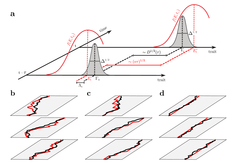
We consider the evolution of the trait E𝐸E under genetic drift, genomic mutations, and natural selection, which is given by a trait-dependent fitness seascape f(E,t)𝑓𝐸𝑡f(E,t) that changes on macro-evolutionary time scales. This process is illustrated in Fig. 1: At a given evolutionary time, the trait distribution in a population has mean Γ(t)Γ𝑡\Gamma(t), diversity Δ(t)Δ𝑡\Delta(t), and is positioned at a distance Λ(t)Γ(t)E(t)Λ𝑡Γ𝑡superscript𝐸𝑡\Lambda(t)\equiv\Gamma(t)-E^{*}(t) from the optimal trait value. The trait distribution follows the moving fitness peak, building up a trait divergence

D(1)(t,τ)=(Γ(t)Γ(tτ))2superscript𝐷1𝑡𝜏superscriptΓ𝑡Γ𝑡𝜏2D^{(1)}(t,\tau)=(\Gamma(t)-\Gamma(t-\tau))^{2} (4)

between an ancestral population at time tτ𝑡𝜏t-\tau and its descendent population at time t𝑡t in a given lineage. In the same way, we can define the trait divergence between two descendent populations at time t𝑡t that have evolved independently from a common ancestor population at time tτ/2𝑡𝜏2t-\tau/2,

D(2)(t,τ)=(Γ1(t)Γ2(t))2.superscript𝐷2𝑡𝜏superscriptsubscriptΓ1𝑡subscriptΓ2𝑡2D^{(2)}(t,\tau)=(\Gamma_{1}(t)-\Gamma_{2}(t))^{2}. (5)

In a suitably defined ensemble of parallel-evolving populations, the expectation values of these divergences, D(κ)(τ)delimited-⟨⟩superscript𝐷𝜅𝜏\langle D^{(\kappa)}(\tau)\rangle (κ=1,2𝜅12\kappa=1,2), depend only on the divergence time τ𝜏\tau. The asymptotic divergence for long times is just twice the trait variance across populations,

limτD(κ)(τ)=2(ΓΓ)2(κ=1,2).subscript𝜏delimited-⟨⟩superscript𝐷𝜅𝜏2delimited-⟨⟩superscriptΓdelimited-⟨⟩Γ2𝜅12\lim_{\tau\to\infty}\langle D^{(\kappa)}(\tau)\rangle=2\langle(\Gamma-\langle\Gamma\rangle)^{2}\rangle\hskip 28.45274pt(\kappa=1,2). (6)

In particular, the quantity E02superscriptsubscript𝐸02E_{0}^{2} defined in (2) is the trait variance in an ensemble of random genotypes, which results from neutral evolution (with averages 0subscriptdelimited-⟨⟩0\langle\dots\rangle_{0} marked by a subscript) at low mutation rates, E02=limμ0(ΓΓ0)20superscriptsubscript𝐸02subscript𝜇0subscriptdelimited-⟨⟩superscriptΓsubscriptdelimited-⟨⟩Γ020E_{0}^{2}=\lim_{\mu\to 0}\langle(\Gamma-\langle\Gamma\rangle_{0})^{2}\rangle_{0}. For finite times, however, the statistics of the single-lineage divergence D(1)superscript𝐷1D^{(1)} and the cross-lineage divergence D(2)superscript𝐷2D^{(2)} differ from each other in an adaptive process. As we will discuss in detail below, this is a manifestation of the non-equilibrium evolutionary dynamics in a fitness seascape. In contrast, evolutionary equilibrium in a fitness landscape dictates D(1)(τ)eq=D(2)(τ)eqsubscriptdelimited-⟨⟩superscript𝐷1𝜏eqsubscriptdelimited-⟨⟩superscript𝐷2𝜏eq\langle D^{(1)}(\tau)\rangle_{\rm eq}={\langle}D^{(2)}(\tau){\rangle}_{\rm eq} by detailed balance.

Refer to caption
Figure 1: Adaptive evolution of a quantitative trait. (a) Evolution of the distribution of trait values 𝒲(E,t)𝒲𝐸𝑡{\cal W}(E,t) (gray curves) in a given population subject to a single-peak fitness seascape f(E,t)𝑓𝐸𝑡f(E,t) (red curves). At a given time t𝑡t, the population has a trait distribution 𝒲(E,t)𝒲𝐸𝑡{\cal W}(E,t) with mean Γ(t)Γ𝑡\Gamma(t) and diversity Δ(t)Δ𝑡\Delta(t), and is positioned at a distance Λ(t)=Γ(t)E(t)Λ𝑡Γ𝑡superscript𝐸𝑡\Lambda(t)=\Gamma(t)-E^{*}(t) from the fitness peak. The population follows the moving fitness peak and builds up a trait divergence D(1)(t,τ)=(Γ(t)Γ(tτ))2superscript𝐷1𝑡𝜏superscriptΓ𝑡Γ𝑡𝜏2D^{(1)}(t,\tau)=(\Gamma(t)-\Gamma(t-\tau))^{2} between the ancestral state at time tτ𝑡𝜏t-\tau and the descendent state at time t𝑡t. The divergence D(2)(t,τ)superscript𝐷2𝑡𝜏D^{(2)}(t,\tau) between two descendent populations with a common ancestor at time tτ/2𝑡𝜏2t-\tau/2 can be defined in an analogous way; see eqs. (4) and (5). (b–d) Evolutionary population ensembles, each represented by three sample populations. In a given population, a realization of a single-peak fitness seascape specifies a lineage-specific optimal trait value that depends on evolutionary time, E(t)superscript𝐸𝑡E^{*}(t) (red line). The population mean trait, Γ(t)Γ𝑡\Gamma(t) (black line), adapts to the moving fitness peak with additional lineage-specific fluctuations due to mutations and genetic drift. The adaptive process is shown for three cases of fitness seascapes: (b) Diffusive fitness seascape: Incremental changes in the optimal trait value reflect adaptive pressure caused by continuous ecological changes. The function E(t)superscript𝐸𝑡E^{*}(t) follows an Ornstein-Uhlenback random walk in the trait coordinate. (c) Punctuated fitness seascape: Sudden changes in the optimal trait value reflect adaptive pressure caused by major, discrete ecological events. The function E(t)superscript𝐸𝑡E^{*}(t) is described by a Poisson jump process in the trait coordinate. We show that both types of fitness seascapes lead to a solvable, non-equilibrium joint statistics of ΓΓ\Gamma and Esuperscript𝐸E^{*}. (d) Fitness landscape: Each population has a time-independent optimal trait value Esuperscript𝐸E^{*} and reaches an evolutionary (selection-mutation-drift) equilibrium [1].

As shown in a previous companion paper [1], the evolutionary dynamics of a quantitative trait in a fitness seascape can be described in good approximation by diffusion equations for its mean and its diversity,

tQ(Γ,t|F1)𝑡𝑄Γconditional𝑡subscript𝐹1\displaystyle\frac{\partial}{\partial t}Q(\Gamma,t\,|\,F_{1}) =\displaystyle= [gΓΓ2N2Γ2Γ(mΓ+gΓΓF1(Γ,t)Γ)]Q(Γ,t|F1),delimited-[]superscript𝑔ΓΓ2𝑁superscript2superscriptΓ2Γsuperscript𝑚Γsuperscript𝑔ΓΓsubscript𝐹1Γ𝑡Γ𝑄Γconditional𝑡subscript𝐹1\displaystyle\left[\frac{g^{\Gamma\Gamma}}{2N}\frac{\partial^{2}}{\partial\Gamma^{2}}-\frac{\partial}{\partial\Gamma}\left(m^{\Gamma}+g^{\Gamma\Gamma}\frac{\partial F_{1}(\Gamma,t)}{\partial\Gamma}\right)\right]Q(\Gamma,t\,|\,F_{1}), (7)
tQ(Δ,t|F2)𝑡𝑄Δconditional𝑡subscript𝐹2\displaystyle\frac{\partial}{\partial t}Q(\Delta,t\,|\,F_{2}) =\displaystyle= [gΔΔ2N2Δ2Δ(mΔ+gΔΔF2(Δ,t)Δ)]Q(Δ,t|F2),delimited-[]superscript𝑔ΔΔ2𝑁superscript2superscriptΔ2Δsuperscript𝑚Δsuperscript𝑔ΔΔsubscript𝐹2Δ𝑡Δ𝑄Δconditional𝑡subscript𝐹2\displaystyle\left[\frac{g^{\Delta\Delta}}{2N}\frac{\partial^{2}}{\partial\Delta^{2}}-\frac{\partial}{\partial\Delta}\left(m^{\Delta}+g^{\Delta\Delta}\frac{\partial F_{2}(\Delta,t)}{\partial\Delta}\right)\right]Q(\Delta,t\,|\,F_{2}), (8)

which are projections of the Kimura diffusion equation [19, 20] from genotypes onto the phenotype space. The distributions Q(Γ,t|F1)𝑄Γconditional𝑡subscript𝐹1Q(\Gamma,t\,|\,F_{1}) and Q(Δ,t|F2)𝑄Δconditional𝑡subscript𝐹2Q(\Delta,t\,|\,F_{2}) describe an ensemble of populations evolving in the same fitness seascape f(E,t)𝑓𝐸𝑡f(E,t). These dynamics involve the fitness seascape components

F1(Γ,t)subscript𝐹1Γ𝑡\displaystyle F_{1}(\Gamma,t) =\displaystyle= f(Γ,t)+f′′(Γ,t)×dΔΔQ2(Δ,t|F2),𝑓Γ𝑡superscript𝑓′′Γ𝑡dΔΔsubscript𝑄2Δconditional𝑡subscript𝐹2\displaystyle f(\Gamma,t)+f^{\prime\prime}(\Gamma,t)\times\int\!\text{d}\Delta\,\Delta\,Q_{2}(\Delta,t\,|\,F_{2}), (9)
F2(Δ,t)subscript𝐹2Δ𝑡\displaystyle F_{2}(\Delta,t) =\displaystyle= Δ×dΓf′′(Γ,t)Q(Γ,t|F1),ΔdΓsuperscript𝑓′′Γ𝑡𝑄Γconditional𝑡subscript𝐹1\displaystyle\Delta\times\int\!\text{d}\Gamma\,f^{\prime\prime}(\Gamma,t)\,Q(\Gamma,t\,|\,F_{1}), (10)

which are projections of the mean population fitness

f¯(t)dEf(E,t)𝒲(E,t)=f(Γ,t)+12Δf′′(Γ,t)+¯𝑓𝑡d𝐸𝑓𝐸𝑡𝒲𝐸𝑡𝑓Γ𝑡12Δsuperscript𝑓′′Γ𝑡\overline{f}(t)\equiv\int\text{d}E\,f(E,t)\,{\cal W}(E,t)=f(\Gamma,t)+\frac{1}{2}\Delta f^{\prime\prime}(\Gamma,t)+\dots (11)

onto the marginal variables ΓΓ\Gamma and ΔΔ\Delta. Genetic drift enters through the diffusion coefficients gΓΓ=ΔdΔΔQ(Δ,t|F2)superscript𝑔ΓΓdelimited-⟨⟩ΔdΔΔ𝑄Δconditional𝑡subscript𝐹2g^{\Gamma\Gamma}=\langle\Delta\rangle\equiv\int\!\text{d}\Delta\,\Delta\,Q(\Delta,t\,|\,F_{2}) and gΔΔ=2Δ2superscript𝑔ΔΔ2superscriptΔ2g^{\Delta\Delta}=2\Delta^{2}, mutations through the mutation coefficients mΓ=2μ(ΓΓ0)superscript𝑚Γ2𝜇ΓsubscriptΓ0m^{\Gamma}=-2\mu(\Gamma-\Gamma_{0}) and mΔ=4μ(ΔE02)Δ/Nsuperscript𝑚Δ4𝜇Δsuperscriptsubscript𝐸02Δ𝑁m^{\Delta}=-4\mu(\Delta-E_{0}^{2})-\Delta/N; these coefficients depend on the effective population size N𝑁N and the point mutation rate μ𝜇\mu. The diffusion equations (7) and (8) are coupled through the fitness components (9) and (10) and through the diffusion coefficient gΓΓsuperscript𝑔ΓΓg^{\Gamma\Gamma}. In the absence of direct selection on the trait mean, i.e. for F1(Γ,t)=0subscript𝐹1Γ𝑡0F_{1}(\Gamma,t)=0, eq. (7) describes a “quasi-neutral” diffusion of the trait mean, which depends the full drift term gΓΓ=Δ(c)superscript𝑔ΓΓdelimited-⟨⟩Δ𝑐g^{\Gamma\Gamma}=\langle\Delta\rangle(c) under selection. This dynamics defines a characteristic time scale

τ~2NE02Δ.~𝜏2𝑁superscriptsubscript𝐸02delimited-⟨⟩Δ\tilde{\tau}\equiv\frac{2NE_{0}^{2}}{\langle\Delta\rangle}. (12)

Recombination between the trait loci induces a crossover between selection on entire genotypes and selection on individual alleles [21, 22]. This affects the form of the diffusive dynamics of ΔΔ\Delta and, hence, the coefficients of the diffusion equation for ΓΓ\Gamma. However, these changes have only a small effect on the statistics of ΓΓ\Gamma over a wide range of evolutionary parameters [1].

In the special case of a time-independent fitness landscape f(E)𝑓𝐸f(E), the diffusive dynamics of trait mean and diversity leads to evolutionary equilibria of a Boltzmann form [1],

Qeq(Γ|F1)subscript𝑄eqconditionalΓsubscript𝐹1\displaystyle Q_{\rm eq}(\Gamma\,|\,F_{1}) =\displaystyle= 1ZΓQ~0(Γ)exp[2NF1(Γ)],1subscript𝑍Γsubscript~𝑄0Γ2𝑁subscript𝐹1Γ\displaystyle\frac{1}{Z_{\Gamma}}\,\tilde{Q}_{0}(\Gamma)\,\exp[2NF_{1}(\Gamma)], (13)
Qeq(Δ|F2)subscript𝑄eqconditionalΔsubscript𝐹2\displaystyle Q_{\rm eq}(\Delta\,|\,F_{2}) =\displaystyle= 1ZΔQ0(Δ)exp[2NF2(Δ)],1subscript𝑍Δsubscript𝑄0Δ2𝑁subscript𝐹2Δ\displaystyle\frac{1}{Z_{\Delta}}\,Q_{0}(\Delta)\,\exp[2NF_{2}(\Delta)], (14)

where ZΓsubscript𝑍ΓZ_{\Gamma} and ZΔsubscript𝑍ΔZ_{\Delta} are normalization constants. The equilibrium distributions under selection build on the quasi-neutral distribution of the trait mean, Q~0(Γ)exp[2μN(ΓΓ0)2/Δ]similar-tosubscript~𝑄0Γ2𝜇𝑁superscriptΓsubscriptΓ02delimited-⟨⟩Δ\tilde{Q}_{0}(\Gamma)\sim\exp[-2\mu N(\Gamma-\Gamma_{0})^{2}/\langle\Delta\rangle], and on the neutral diversity distribution Q0(Δ)subscript𝑄0ΔQ_{0}(\Delta) (see also section 3.3). We note that evolutionary equilibrium in a static fitness landscape is limited to the marginal distributions Qeq(Γ|F1)subscript𝑄eqconditionalΓsubscript𝐹1Q_{\rm eq}(\Gamma\,|\,F_{1}) and Qeq(Δ|F2)subscript𝑄eqconditionalΔsubscript𝐹2Q_{\rm eq}(\Delta\,|\,F_{2}), while the joint distribution Q(Γ,Δ|f)𝑄ΓconditionalΔ𝑓Q(\Gamma,\Delta|f) reaches a non-equilibrium stationary state [1]. In the limit of low mutation rates, the Boltzmann distribution (13) describes an asymptotic selection-drift equilibrium Qeq(E|F1)Q0(E)exp[2NF(E)]similar-tosubscript𝑄eqconditional𝐸subscript𝐹1subscript𝑄0𝐸2𝑁𝐹𝐸Q_{\rm eq}(E|F_{1})\sim Q_{0}(E)\exp[2NF(E)]; the trait values E𝐸E are predominantly monomorphic in a population and they change by substitutions at individual trait loci [23, 24, 1].

2.2 Stochastic seascape models

For a generic fitness seascape f(E,t)𝑓𝐸𝑡f(E,t), the diffusion equations (7) and (8) do not have a closed analytical solution. At the same time, we are often not interested in the detailed history of fitness peak displacements and the resulting trait changes. To describe generic features of adaptive processes, we now introduce solvable stochastic models of the seascape dynamics and link broad features of these models to statistical observables of adapting populations.

In this paper, we restrict our analysis to single-peak fitness seascapes of the form

f(E,t)=fc0(EE(t))2.𝑓𝐸𝑡superscript𝑓subscript𝑐0superscript𝐸superscript𝐸𝑡2f(E,t)=f^{*}-c_{0}\big{(}E-E^{*}(t)\big{)}^{2}. (15)

Despite its simple form, the fitness function (15) covers a broad spectrum of interesting selection scenarios [25]. For constant trait optimum Esuperscript𝐸E^{*}, it is a time-honored model of stabilizing selection. [2, 6, 10, 25, 23, 26, 27, 28, 29, 14]. Nearly all known examples of empirical fitness landscapes for molecular quantitative traits are of single-peak [30] or mesa-shaped [31, 26, 32, 33, 34] forms. Mesa landscapes describe directional selection with diminishing return: they contain a fitness flank on one side of a characteristic “rim” value Esuperscript𝐸E^{*} and flatten to a plateau of maximal fitness on the other side. Furthermore, trait values on the fitness plateau tend to be encoded by far fewer genotypes than low-fitness values. This differential coverage of the genotype-phenotype map turns out to generate an effective second flank of the fitness landscape, which makes our subsequent theory applicable to mesa landscapes as well [25]. We refer to the scaled parameter

c=2NE02c0𝑐2𝑁superscriptsubscript𝐸02subscript𝑐0c=2NE_{0}^{2}c_{0} (16)

as the stabilizing strength of a fitness landscape. This dimensionless quantity has a simple interpretation: it equals the ratio of the neutral trait variance E02superscriptsubscript𝐸02E_{0}^{2} and the weakly deleterious trait variance around the fitness peak, which, by definition, produces a fitness drop 1/(2N)absent12𝑁\leq 1/(2N) below the maximum fsuperscript𝑓f^{*}. As shown in ref. [1], the mutation-selection-drift dynamics of a quantitative trait in a single-peak fitness landscape leads to evolutionary equilibrium with a characteristic equilibration time

τeq(c)subscript𝜏eq𝑐\displaystyle\tau_{\rm eq}(c) =\displaystyle= 1μ+cτ~1(c){μ1 for c1,(cτ~(c))1 for c1,similar-to-or-equals1𝜇𝑐superscript~𝜏1𝑐casessuperscript𝜇1 for c1,superscript𝑐~𝜏𝑐1 for c1,\displaystyle\frac{1}{\mu+c\tilde{\tau}^{-1}(c)}\simeq\left\{\begin{array}[]{ll}\mu^{-1}&\mbox{ for $c\lesssim 1$,}\\ (c\tilde{\tau}(c))^{-1}&\mbox{ for $c\gtrsim 1$,}\end{array}\right. (19)

where τ~(c)~𝜏𝑐\tilde{\tau}(c) is the quasi-neutral drift time defined in eq. (12).

For time-dependent E(t)superscript𝐸𝑡E^{*}(t), eq. (15) becomes a fitness seascape model [12, 13, 14]. At any given evolutionary time, this model describes stabilizing selection of strength c𝑐c towards an optimal trait value E(t)superscript𝐸𝑡E^{*}(t). In addition, the changes of E(t)superscript𝐸𝑡E^{*}(t) over macro-evolutionary periods introduce directional selection on the trait and generate adaptive evolution. The form (15) of a fitness seascape assumes the stabilizing strength c𝑐c to remain constant over time. As discussed in section 2.3, this assumption leads to an important computational simplification: only the trait mean ΓΓ\Gamma adapts to the moving fitness peak, while the diversity ΔΔ\Delta remains at evolutionary equilibrium. However, generalizing of our model to a time-dependent stabilizing strength c(t)𝑐𝑡c(t) is straightforward and is briefly discussed below. We consider two minimal models of seascape dynamics:

Diffusive fitness seascapes.

In this model, the fitness optimum E(t)superscript𝐸𝑡E^{*}(t) performs an Ornstein-Uhlenbeck random walk with diffusion constant υ0subscript𝜐0\upsilon_{0}, average value \mathcal{E} and stationary mean square deviation r02superscriptsubscript𝑟02r_{0}^{2}. The scaled parameters

υ=υ0E02,r2=r02E02,formulae-sequence𝜐subscript𝜐0superscriptsubscript𝐸02superscript𝑟2superscriptsubscript𝑟02superscriptsubscript𝐸02\upsilon=\frac{\upsilon_{0}}{E_{0}^{2}},\hskip 28.45274ptr^{2}=\frac{r_{0}^{2}}{E_{0}^{2}}, (20)

will be called the driving rate and the driving span of a fitness seascape. Different realizations of this random walk with the same set of parameters are shown in Fig. 1(b). The distribution of optimum trait values, R(E,t)𝑅superscript𝐸𝑡R(E^{*},t), follows a diffusion equation,

tR(E,t)=υE02E[E+1r2E02(E)]R(E,t).𝑡𝑅superscript𝐸𝑡𝜐superscriptsubscript𝐸02superscript𝐸delimited-[]superscript𝐸1superscript𝑟2superscriptsubscript𝐸02superscript𝐸𝑅superscript𝐸𝑡\frac{\partial}{\partial t}R(E^{*},t)={\upsilon E_{0}^{2}}\,\frac{\partial}{\partial E^{*}}\left[\frac{\partial}{\partial{E^{*}}}+\frac{1}{r^{2}E_{0}^{2}}(E^{*}-\mathcal{E})\right]R(E^{*},t). (21)

This dynamics leads to a seascape ensemble, which is characterized by an expected peak divergence

(E(t)E(t+τ))2=2r2E02(1eτ/τsat(υ,r2))delimited-⟨⟩superscriptsuperscript𝐸𝑡superscript𝐸𝑡𝜏22superscript𝑟2superscriptsubscript𝐸021superscripte𝜏subscript𝜏sat𝜐superscript𝑟2\big{\langle}(E^{*}(t)-E^{*}(t+\tau))^{2}\big{\rangle}=2r^{2}E_{0}^{2}\left(1-{\rm e}^{-\tau/\tau_{\rm sat}(\upsilon,r^{2})}\right) (22)

with the saturation time

τsat(υ,r2)=r2υ,subscript𝜏sat𝜐superscript𝑟2superscript𝑟2𝜐\tau_{\rm sat}(\upsilon,r^{2})=\frac{r^{2}}{\upsilon}, (23)

and by an equilibrium distribution

Req(E)=12πr2E02exp[12(E)2r2E02]subscript𝑅eqsuperscript𝐸12𝜋superscript𝑟2superscriptsubscript𝐸0212superscriptsuperscript𝐸2superscript𝑟2superscriptsubscript𝐸02R_{\rm eq}(E^{*})=\frac{1}{\sqrt{2\pi r^{2}E_{0}^{2}}}\,\exp\left[-\frac{1}{2}\frac{(E^{*}-\mathcal{E})^{2}}{r^{2}E_{0}^{2}}\right] (24)

of optimal trait values. Diffusive seascapes models of this form describe continuous adaptive pressure due to incremental ecological changes that affect the optimal trait value E(t)superscript𝐸𝑡E^{*}(t). We assume that typical optimal trait values fall into the neutral trait repertoire given by eq. (2), which implies that the scaled driving span r2superscript𝑟2r^{2} is at most of order 1.

Punctuated fitness seascapes.

In this model, the fitness optimum performs a Poisson jump process with jump rate τsat1(v,r2)=υ/r2subscriptsuperscript𝜏1sat𝑣superscript𝑟2𝜐superscript𝑟2\tau^{-1}_{\rm sat}(v,r^{2})=\upsilon/r^{2}, by which successive values of Esuperscript𝐸E^{*} are drawn independently from the distribution Req(E)subscript𝑅eqsuperscript𝐸R_{\rm eq}(E^{*}), given by (24). Different realizations of this process are shown in Fig. 1(c). Fitness jumps may result from discrete ecological events such as major migrations or speciations. The Poisson jump process is described by the evolution equation

tR(E,t)=υr2[Req(E)R(E,t)].𝑡𝑅superscript𝐸𝑡𝜐superscript𝑟2delimited-[]subscript𝑅eqsuperscript𝐸𝑅superscript𝐸𝑡\frac{\partial}{\partial t}R(E^{*},t)=\frac{\upsilon}{r^{2}}\,\big{[}R_{\rm eq}(E^{*})-R(E^{*},t)]. (25)

It has the same time-dependent expected peak divergence (22) and the same equilibrium distribution (24) as the diffusion process (21) with same driving parameters (20). The difference between the jump process and the diffusion process lies in the anomalous scaling of higher moments,

(E(t)E(t+τ))kdelimited-⟨⟩superscriptsuperscript𝐸𝑡superscript𝐸𝑡𝜏𝑘\displaystyle\big{\langle}(E^{*}(t)-E^{*}(t+\tau))^{k}\big{\rangle} similar-to\displaystyle\sim E0krk2υτ for k=2,4, and ττsat(υ,r2).superscriptsubscript𝐸0𝑘superscript𝑟𝑘2𝜐𝜏 for k=2,4, and ττsat(υ,r2).\displaystyle E_{0}^{k}r^{k-2}\upsilon\tau\hskip 28.45274pt\mbox{ for $k=2,4,\dots$ and $\tau\ll\tau_{\rm sat}(\upsilon,r^{2})$.} (26)

This scaling is shared by simple models of turbulence; see, e.g., ref. [35].


In both types of fitness seascape, we distinguish two dynamical selection regimes:

  • Macro-evolutionary fitness seascapes are defined by the condition τsat(v,r2)τeq(c)greater-than-or-equivalent-tosubscript𝜏sat𝑣superscript𝑟2subscript𝜏eq𝑐\tau_{\rm sat}(v,r^{2})\gtrsim\tau_{\rm eq}(c). As discussed in detail below, such seascapes keep the trait mean always close to equilibrium and induce an adaptive response linear in the driving rate υ𝜐\upsilon. The limit υ0𝜐0\upsilon\to 0 describes an ensemble of quenched population-specific fitness landscapes with a distribution of optimal trait values given by eq. (24); see Fig. 1(d).

  • Micro-evolutionary fitness seascapes have τsat(v,r2)τeq(c)less-than-or-similar-tosubscript𝜏sat𝑣superscript𝑟2subscript𝜏eq𝑐\tau_{\rm sat}(v,r^{2})\lesssim\tau_{\rm eq}(c) and delineate a regime of reduced adaptive response, where the evolution of the trait mean gradually decouples from that of the fitness seascape. In the asymptotic fast-driving regime (υr2/τeq(c)much-greater-than𝜐superscript𝑟2subscript𝜏eq𝑐\upsilon\gg r^{2}/\tau_{\rm eq}(c)), the adaptation of the trait is completely suppressed. In this regime, we can average over the fitness fluctuations and describe the macro-evolution of the trait in terms of an effective fitness landscape with an optimal trait value \mathcal{E}.

2.3 Joint dynamics of trait and selection

We now combine the diffusive dynamics of quantitative traits in a given fitness seascape, which is given by eqs. (7) and (8), and the seascape dynamics (21) or (25) into a stochastic model of adaptive evolution. The statistical ensemble generated by this model is illustrated in Fig. 1(b-d): Each population evolves in a specific realization of the fitness seascape, which is given by a history of peak values E(t)superscript𝐸𝑡E^{*}(t). Its trait mean Γ(t)Γ𝑡\Gamma(t) follows the moving fitness peak with fluctuations due to mutations and genetic drift. The ensemble of populations contains, in addition, the stochastic differences between realizations of the fitness seascape. The statistics of this ensemble involves combined averages over both kinds of fluctuations, which are denoted by angular brackets delimited-⟨⟩{\langle}...{\rangle}.

The population ensemble can be described by a joint distribution of mean and optimum trait values, Q(Γ,E,t)=Q(Γ,t|E)R(E,t)𝑄Γsuperscript𝐸𝑡𝑄Γconditional𝑡superscript𝐸𝑅superscript𝐸𝑡Q(\Gamma,E^{*},t)=Q(\Gamma,t\,|\,E^{*})R(E^{*},t). Using eqs. (7) and (21) together with the projection of the fitness seascape,

F1(Γ|E)=fcNE02ΔcE02(ΓE)2,subscript𝐹1conditionalΓsuperscript𝐸superscript𝑓𝑐𝑁superscriptsubscript𝐸02delimited-⟨⟩Δ𝑐superscriptsubscript𝐸02superscriptΓsuperscript𝐸2F_{1}(\Gamma\,|\,E^{*})=f^{*}-\frac{c}{NE_{0}^{2}}{\langle}\Delta{\rangle}-\frac{c}{E_{0}^{2}}\big{(}\Gamma-E^{*}\big{)}^{2}, (27)

given by eqs. (9) and (15), we obtain the evolution equation for the joint distribution in a diffusive seascape,

tQ(Γ,E,t)𝑡𝑄Γsuperscript𝐸𝑡\displaystyle{\frac{\partial}{\partial t}Q(\Gamma,E^{*},t)} =\displaystyle= [gΓΓ2N2Γ2Γ(mΓgΓΓ2cE02(ΓE))+υE022E2+υr2E(E)]Q(Γ,E,t),delimited-[]superscript𝑔ΓΓ2𝑁superscript2superscriptΓ2Γsuperscript𝑚Γsuperscript𝑔ΓΓ2𝑐superscriptsubscript𝐸02Γsuperscript𝐸𝜐superscriptsubscript𝐸02superscript2superscript𝐸absent2𝜐superscript𝑟2superscript𝐸superscript𝐸𝑄Γsuperscript𝐸𝑡\displaystyle\left[\frac{g^{\Gamma\Gamma}}{2N}\frac{\partial^{2}}{\partial\Gamma^{2}}-\frac{\partial}{\partial\Gamma}\left(m^{\Gamma}-g^{\Gamma\Gamma}\frac{2c}{E_{0}^{2}}(\Gamma-E^{*})\right)\right.+\left.\frac{\upsilon}{E_{0}^{2}}\frac{\partial^{2}}{\partial E^{*2}}+\frac{\upsilon}{r^{2}}\frac{\partial}{\partial{E^{*}}}(E^{*}-\mathcal{E})\right]Q(\Gamma,E^{*},t),

with gΓΓ=Δsuperscript𝑔ΓΓdelimited-⟨⟩Δg^{\Gamma\Gamma}=\langle\Delta\rangle and mΓ=2μ(ΓΓ0)superscript𝑚Γ2𝜇ΓsubscriptΓ0m^{\Gamma}=-2\mu(\Gamma-\Gamma_{0}). Note that the differential operator in eq. (LABEL:diffGammaEstar) is asymmetric: the trait optimum Esuperscript𝐸E^{*} follows an independent stochastic dynamics, but the trait mean ΓΓ\Gamma is coupled to Esuperscript𝐸E^{*}. This asymmetry reflects the causal relation between selection and adaptive response: the trait mean Γ(t)Γ𝑡\Gamma(t) follows the moving fitness peak, as shown in Fig. 1(b,c). As a consequence, the joint evolution equation (LABEL:diffGammaEstar) leads to a non-equilibrium stationary distribution Qstat(Γ,E)subscript𝑄statΓsuperscript𝐸Q_{\rm stat}(\Gamma,E^{*}), although the marginal seascape dynamics (21) reaches an equilibrium state. Only in the fitness landscape limit (υ0𝜐0\upsilon\to 0), the evolution of the trait mean reaches evolutionary equilibrium. In the next section, we will obtain explicit solutions for the non-equilibrium distribution Qstat(Γ,E)subscript𝑄statΓsuperscript𝐸Q_{\rm stat}(\Gamma,E^{*}) and its equilibrium limit. The case of a punctuated fitness seascape is treated in Appendix A, where we solve the Langevin equations for ΓΓ\Gamma and Esuperscript𝐸E^{*} to obtain the first and second moments of Q(Γ,E,t)𝑄Γsuperscript𝐸𝑡Q(\Gamma,E^{*},t).

The trait diversity evolves under the projected fitness function

F2(Δ|c)=cNE02Δ,subscript𝐹2conditionalΔ𝑐𝑐𝑁superscriptsubscript𝐸02ΔF_{2}(\Delta\,|\,c)=-\frac{c}{NE_{0}^{2}}\,\Delta, (29)

given by eqs. (15) and (10). In a fitness seascapes with a constant stabilizing strength c𝑐c, this function is time-independent. The dynamics of the trait diversity (8) decouples from the adaptive evolution of the trait mean and leads an evolutionary equilibrium Qeq(Δ|c)subscript𝑄eqconditionalΔ𝑐Q_{\rm eq}(\Delta\,|\,c) of the form (14). As detailed in Section 3.3, the equilibrium assumption for the trait diversity holds for most adaptive processes in a fitness seascape of the form (15). However, we can generalize our seascape models to include a time-dependent stabilizing strength c(t)𝑐𝑡c(t). This leads to generic adaptive evolution of both, ΓΓ\Gamma and ΔΔ\Delta, which is described by a coupled non-equilibrium stationary distribution Qstat(Γ,Δ,E,c)subscript𝑄statΓΔsuperscript𝐸𝑐Q_{\rm stat}(\Gamma,\Delta,E^{*},c).

3 Adaptive evolution in a single-peak fitness seascape

In this section, we develop the key analytical results of this paper. We provide an explicit solution for the non-equilibrium joint distribution of mean and optimal trait in a diffusive seascape, Qstat(Γ,E)subscript𝑄statΓsuperscript𝐸Q_{\rm stat}(\Gamma,E^{*}); the case of punctuated seascapes is treated in Appendix A. These solutions describe a stationary ensembles of adapting populations. We derive an expression for the expected time-dependent trait divergence in these ensembles, which holds for both seascape models. Finally, we juxtapose the adaptive behavior of the trait mean with the equilibrium statistics of the trait diversity, which emerges in good approximation for most fitness seascape of constant stabilizing strength. Our analytical results are supported by simulations for diffusive and punctuated fitness seascapes.

3.1 Stationary distribution of mean and optimal trait

In a diffusive fitness seascape, the evolution equation (LABEL:diffGammaEstar) has a stationary solution of bivariate Gaussian form,

Qstat(Γ,E)=1Zexp[12(Γ^E^)T𝚺1(Γ^E^)],subscript𝑄statΓsuperscript𝐸1𝑍12superscriptmatrix^Γsuperscript^𝐸𝑇superscript𝚺1matrix^Γsuperscript^𝐸\displaystyle Q_{\rm stat}(\Gamma,E^{*})=\frac{1}{Z}\exp\left[-\frac{1}{2}\begin{pmatrix}\hat{\Gamma}\\ \hat{E}^{*}\end{pmatrix}^{T}\mathbf{\Sigma}^{-1}\begin{pmatrix}\hat{\Gamma}\\ \hat{E}^{*}\end{pmatrix}\right], (30)

with the expectation values

(ΓE)delimited-⟨⟩Γdelimited-⟨⟩superscript𝐸\displaystyle\left(\begin{array}[]{c}\langle\Gamma\rangle\\ \langle E^{*}\rangle\end{array}\right) \displaystyle\equiv dΓdE(ΓE)Qstat(Γ,E)dΓdsuperscript𝐸matrixΓsuperscript𝐸subscript𝑄statΓsuperscript𝐸\displaystyle\int\!\text{d}\Gamma\text{d}E^{*}\,\begin{pmatrix}\Gamma\\ E^{*}\end{pmatrix}Q_{\rm stat}(\Gamma,E^{*}) (33)
=\displaystyle= (w(c)+(1w(c))Γ0),𝑤𝑐1𝑤𝑐subscriptΓ0\displaystyle\left(\begin{array}[]{c}w(c)\,\mathcal{E}+(1-w(c))\,\Gamma_{0}\\ \mathcal{E}\end{array}\right), (36)

and the covariance matrix

𝚺=(Γ^2Γ^E^Γ^E^E^2)𝚺matrixdelimited-⟨⟩superscript^Γ2delimited-⟨⟩^Γsuperscript^𝐸delimited-⟨⟩^Γsuperscript^𝐸delimited-⟨⟩superscript^𝐸absent2\displaystyle\mathbf{\Sigma}=\begin{pmatrix}{\langle}\hat{\Gamma}^{2}{\rangle}&{{\langle}}\hat{\Gamma}\hat{E}^{*}{{\rangle}}\\ {{\langle}}\hat{\Gamma}\hat{E}^{*}{{\rangle}}&\langle\hat{E}^{*2}\rangle\end{pmatrix} \displaystyle\equiv dΓdE(Γ^2Γ^E^Γ^E^E^2)Qstat(Γ,E)dΓdsuperscript𝐸matrixsuperscript^Γ2^Γsuperscript^𝐸^Γsuperscript^𝐸superscript^𝐸absent2subscript𝑄statΓsuperscript𝐸\displaystyle\int\!\text{d}\Gamma\text{d}E^{*}\,\begin{pmatrix}\hat{\Gamma}^{2}&\hat{\Gamma}\hat{E}^{*}\\ \hat{\Gamma}\hat{E}^{*}&\hat{E}^{*2}\end{pmatrix}Q_{\rm stat}(\Gamma,E^{*}) (37)
=\displaystyle= E02((1/2c)w(c)+r2w(c)w(c,υ,r2)r2w(c,υ,r2)r2w(c,υ,r2)r2),superscriptsubscript𝐸02matrix12𝑐𝑤𝑐superscript𝑟2𝑤𝑐𝑤𝑐𝜐superscript𝑟2superscript𝑟2𝑤𝑐𝜐superscript𝑟2superscript𝑟2𝑤𝑐𝜐superscript𝑟2superscript𝑟2\displaystyle E_{0}^{2}\begin{pmatrix}(1/2c)\,w(c)+r^{2}w(c)w(c,\upsilon,r^{2})&r^{2}w(c,\upsilon,r^{2})\\ r^{2}w(c,\upsilon,r^{2})&r^{2}\end{pmatrix},

where Γ^ΓΓ^ΓΓdelimited-⟨⟩Γ\hat{\Gamma}\equiv\Gamma-\langle\Gamma\rangle and E^Esuperscript^𝐸superscript𝐸\hat{E}^{*}\equiv E^{*}-\mathcal{E}. The stationary distribution Qstat(Γ,E)subscript𝑄statΓsuperscript𝐸Q_{\rm stat}(\Gamma,E^{*}) depends on the parameters that characterize the fitness seascape: the stabilizing strength c𝑐c, the driving rate υ𝜐\upsilon, and the relative driving span r2superscript𝑟2r^{2}, which are defined in eqs. (16) and (20). Together with the effective population size N𝑁N and the point mutation rate μ𝜇\mu, these parameters determine the characteristic time scales of evolution in a fitness seascape, the equilibration time τeq(c)subscript𝜏eq𝑐\tau_{\rm eq}(c) and the saturation time of fitness fluctuations, τsat(υ,r2)subscript𝜏sat𝜐superscript𝑟2\tau_{\rm sat}(\upsilon,r^{2}); see eqs. (19) and (23). The function

w(c,υ,r2)𝑤𝑐𝜐superscript𝑟2\displaystyle w(c,\upsilon,r^{2}) \displaystyle\equiv cδcδ+2θ+Nυ/r2=τeq1(c)μτeq1(c)μ+τsat1(υ,r2),𝑐delimited-⟨⟩𝛿𝑐delimited-⟨⟩𝛿2𝜃𝑁𝜐superscript𝑟2superscriptsubscript𝜏eq1𝑐𝜇superscriptsubscript𝜏eq1𝑐𝜇superscriptsubscript𝜏sat1𝜐superscript𝑟2\displaystyle\frac{c{\langle}\delta{\rangle}}{c{\langle}\delta{\rangle}+2\theta+N\upsilon/r^{2}}=\frac{\tau_{\rm eq}^{-1}(c)-\mu}{\tau_{\rm eq}^{-1}(c)-\mu+\tau_{\rm sat}^{-1}(\upsilon,r^{2})}, (38)

and its equilibrium limit w(c)w(c,υ=0,r2)w(c)\equiv w(c,\upsilon\!=\!0,r^{2}) govern the coupling between the mean and optimal trait. The mutation rate μ𝜇\mu is the inverse of the neutral timescale τeq(0)=μ1subscript𝜏eq0superscript𝜇1\tau_{\rm eq}(0)=\mu^{-1}. These functions depend on the scaled diversity δΔ/E02delimited-⟨⟩𝛿delimited-⟨⟩Δsuperscriptsubscript𝐸02\langle\delta\rangle\equiv\langle\Delta\rangle/E_{0}^{2}, which is given in ref. [1], eqs. (68) – (73), and is restated below in eq. (62). For traits under substantial selection (c1greater-than-or-equivalent-to𝑐1c\gtrsim 1), we can distinguish two dynamical regimes: In macro-evolutionary fitness seascapes, where τsat(υ,r2)τeq(c)2N/(δc)greater-than-or-equivalent-tosubscript𝜏sat𝜐superscript𝑟2subscript𝜏eq𝑐2𝑁delimited-⟨⟩𝛿𝑐\tau_{\rm sat}(\upsilon,r^{2})\gtrsim\tau_{\rm eq}(c)\approx 2N/(\langle\delta\rangle c), this coupling remains close to the equilibrium value w(c)1𝑤𝑐1w(c)\approx 1; micro-evolutionary fitness fluctuations, which have τsat(υ,r2)τeq(c)less-than-or-similar-tosubscript𝜏sat𝜐superscript𝑟2subscript𝜏eq𝑐\tau_{\rm sat}(\upsilon,r^{2})\lesssim\tau_{\rm eq}(c), induce a partial decoupling of mean and optimal trait.

We can also express this crossover in terms of the average square distance between trait mean in the population and optimal trait of the underlying fitness seascape,

Λ2delimited-⟨⟩superscriptΛ2\displaystyle\langle\Lambda^{2}\rangle \displaystyle\equiv dΓdE(ΓE)2Qstat(Γ,E).dΓdsuperscript𝐸superscriptΓsuperscript𝐸2subscript𝑄statΓsuperscript𝐸\displaystyle\int\!\text{d}\Gamma\text{d}E^{*}\,(\Gamma-E^{*})^{2}\,Q_{\rm stat}(\Gamma,E^{*}). (39)

The analytical solution for the scaled quantity λ2Λ2/E02delimited-⟨⟩superscript𝜆2delimited-⟨⟩superscriptΛ2superscriptsubscript𝐸02\langle\lambda^{2}\rangle\equiv\langle\Lambda^{2}\rangle/E_{0}^{2}, follows from eqs. (36) and (37),

λ2(c,υ,r2)delimited-⟨⟩superscript𝜆2𝑐𝜐superscript𝑟2\displaystyle\langle\lambda^{2}\rangle(c,\upsilon,r^{2}) similar-to-or-equals\displaystyle\simeq {λ2eq(c,r2)+υτeq(c)w(c)2[1+𝒪(τeqτsat)],(macroev. seascapes)λeq(c,0)+r2[1𝒪(τsatτeq)],(microev. seascapes),casessubscriptdelimited-⟨⟩superscript𝜆2eq𝑐superscript𝑟2𝜐subscript𝜏eq𝑐𝑤𝑐2delimited-[]1𝒪subscript𝜏eqsubscript𝜏sat(macroev. seascapes)missing-subexpressionmissing-subexpressionsubscriptdelimited-⟨⟩𝜆eq𝑐0superscript𝑟2delimited-[]1𝒪subscript𝜏satsubscript𝜏eq(microev. seascapes)\displaystyle\left\{\begin{array}[]{ll}\langle\lambda^{2}\rangle_{\rm eq}(c,r^{2})+\upsilon\tau_{\rm eq}(c)\dfrac{w(c)}{2}\left[1+\mathcal{O}\left(\dfrac{\tau_{\rm eq}}{\tau_{\rm sat}}\right)\right],&\mbox{(macroev. seascapes)}\\ \\ \langle\lambda\rangle_{\rm eq}(c,0)+r^{2}\Big{[}1-\mathcal{O}\Big{(}\dfrac{\tau_{\rm sat}}{\tau_{\rm eq}}\Big{)}\Big{]},&\mbox{(microev. seascapes)},\end{array}\right. (43)

where

λ2eq(c,r2)subscriptdelimited-⟨⟩superscript𝜆2eq𝑐superscript𝑟2\displaystyle\langle\lambda^{2}\rangle_{\rm eq}(c,r^{2}) =\displaystyle= w(c)2c+(λ20+r2)(1w(c))2𝑤𝑐2𝑐subscriptdelimited-⟨⟩superscript𝜆20superscript𝑟2superscript1𝑤𝑐2\displaystyle\frac{w(c)}{2c}+(\langle\lambda^{2}\rangle_{0}+r^{2})(1-w(c))^{2} (44)
similar-to-or-equals\displaystyle\simeq 12cfor c112𝑐for c1\displaystyle\frac{1}{2c}\hskip 28.45274pt\mbox{for $c\gg 1$}

is the equilibrium average in a fitness landscape. In micro-evolutionary seascapes, this distance remains small, which indicates that the trait distribution 𝒲(E)𝒲𝐸{\cal W}(E) efficiently follows the displacements of the fitness peak. In macro-evolutionary seascapes, the mean square distance λ2delimited-⟨⟩superscript𝜆2\langle\lambda^{2}\rangle becomes comparable to the driving span r2superscript𝑟2r^{2}; that is, the population no longer follows the moving fitness peak in an efficient way.

The distribution Qstat(Γ,E)subscript𝑄statΓsuperscript𝐸Q_{\rm stat}(\Gamma,E^{*}) describes a stationary state that is manifestly out of equilibrium, i.e., it does not have detailed balance. Its probability current

𝐉stat(Γ,E)=(gΓΓ2NΓmΓ+gΓΓ2cNE02(ΓE)υE+υr2(E))Qstat(Γ,E)subscript𝐉statΓsuperscript𝐸matrixsuperscript𝑔ΓΓ2𝑁Γsuperscript𝑚Γsuperscript𝑔ΓΓ2𝑐𝑁superscriptsubscript𝐸02Γsuperscript𝐸𝜐superscript𝐸𝜐superscript𝑟2superscript𝐸subscript𝑄statΓsuperscript𝐸\displaystyle\mathbf{J}_{\rm stat}(\Gamma,E^{*})=-\begin{pmatrix}\dfrac{g^{\Gamma\Gamma}}{2N}\dfrac{\partial}{\partial\Gamma}-m^{\Gamma}+g^{\Gamma\Gamma}\dfrac{2c}{NE_{0}^{2}}(\Gamma-E^{*})\\ \upsilon\dfrac{\partial}{\partial E^{*}}+\dfrac{\upsilon}{r^{2}}(E^{*}-\mathcal{E})\end{pmatrix}Q_{\rm stat}(\Gamma,E^{*}) (48)
{[2υc(Γ^E^(1+1/(2cr2))(Γ^E^))(1+O(τeqτsat))]Qstat(Γ,E),(macroev. seascapes)[cδN(E^2cr2Γ^)(1O(τsatτeq))]Qstat(Γ,E)(microev. seascapes),similar-to-or-equalsabsentcasesdelimited-[]2𝜐𝑐matrix^Γsuperscript^𝐸112𝑐superscript𝑟2^Γsuperscript^𝐸1𝑂subscript𝜏eqsubscript𝜏satsubscript𝑄statΓsuperscript𝐸(macroev. seascapes)missing-subexpressionmissing-subexpressiondelimited-[]𝑐delimited-⟨⟩𝛿𝑁matrixsuperscript^𝐸2𝑐superscript𝑟2^Γ1𝑂subscript𝜏satsubscript𝜏eqsubscript𝑄statΓsuperscript𝐸(microev. seascapes)\displaystyle\simeq\left\{\begin{array}[]{ll}\left[-2\upsilon c\left(\begin{matrix}\hat{\Gamma}-\hat{E}^{*}(1+1/(2cr^{2}))\\ (\hat{\Gamma}-\hat{E}^{*})\end{matrix}\right)\left(1+O\left(\dfrac{\tau_{\rm eq}}{\tau_{\rm sat}}\right)\right)\right]Q_{\rm stat}(\Gamma,E^{*}),&\mbox{(macroev. seascapes)}\\ \\ \left[\dfrac{c{\langle}\delta{\rangle}}{N}\left(\begin{matrix}\hat{E}^{*}\\ -2cr^{2}\hat{\Gamma}\end{matrix}\right)\Big{(}1-O\Big{(}\dfrac{\tau_{\rm sat}}{\tau_{\rm eq}}\Big{)}\Big{)}\right]Q_{\rm stat}(\Gamma,E^{*})&\mbox{(microev. seascapes)},\end{array}\right.

expresses the adaptive motion of the trait mean following the displacements of the fitness peak. The probability current shows a crossover similar to the adaptive part of Λ2delimited-⟨⟩superscriptΛ2{\langle}\Lambda^{2}{\rangle} in (43): it increases linearly for low driving rates and saturates to a constant in the regime of micro-evolutionary fitness fluctuations.

Remarkably, the joint statistics of mean and optimal trait can be associated with evolutionary equilibrium in the limits of low and high driving rates. In the first case, we obtain the equilibrium distribution

Qeq(Γ,E)subscript𝑄eqΓsuperscript𝐸\displaystyle Q_{\rm eq}(\Gamma,E^{*}) =\displaystyle= limυ0Qstat(Γ,E)subscript𝜐0subscript𝑄statΓsuperscript𝐸\displaystyle\lim_{\upsilon\to 0}Q_{\rm stat}(\Gamma,E^{*}) (49)
=\displaystyle= Q~0(Γ)exp[2NF1(Γ|E)]R(E)subscript~𝑄0Γ2𝑁subscript𝐹1conditionalΓsuperscript𝐸𝑅superscript𝐸\displaystyle\tilde{Q}_{0}(\Gamma)\,\exp[2NF_{1}(\Gamma|E^{*})]\;R(E^{*})
=\displaystyle= 1ZΓ2πr2E02exp[2θΔ(ΓΓ0)2cE02(ΓE)212r2E02(E)2],1subscript𝑍Γ2𝜋superscript𝑟2superscriptsubscript𝐸022𝜃delimited-⟨⟩ΔsuperscriptΓsubscriptΓ02𝑐superscriptsubscript𝐸02superscriptΓsuperscript𝐸212superscript𝑟2superscriptsubscript𝐸02superscriptsuperscript𝐸2\displaystyle\frac{1}{Z_{\Gamma}\sqrt{2\pi r^{2}E_{0}^{2}}}\exp\left[-\frac{2\theta}{\langle\Delta\rangle}(\Gamma-\Gamma_{0})^{2}-\frac{c}{E_{0}^{2}}(\Gamma-E^{*})^{2}-\frac{1}{2r^{2}E_{0}^{2}}(E^{*}-\mathcal{E})^{2}\right],

which is the product of a Boltzmann distribution (13) and a quenched weight of the trait optimum Esuperscript𝐸E^{*} given by (24). This distribution satisfies detailed balance; that is, the probability current 𝐉stat(Γ,E)subscript𝐉statΓsuperscript𝐸\mathbf{J}_{\rm stat}(\Gamma,E^{*}) vanishes in the limit υ0𝜐0\upsilon\to 0. In the opposite limit, we obtain the distribution

Q(Γ,E)subscript𝑄Γsuperscript𝐸\displaystyle Q_{\infty}(\Gamma,E^{*}) =\displaystyle= limυQstat(Γ,E)subscript𝜐subscript𝑄statΓsuperscript𝐸\displaystyle\lim_{\upsilon\to\infty}Q_{\rm stat}(\Gamma,E^{*}) (50)
=\displaystyle= Q~0(Γ)exp[2NF1(Γ|)]R(E)subscript~𝑄0Γ2𝑁subscript𝐹1conditionalΓ𝑅superscript𝐸\displaystyle\tilde{Q}_{0}(\Gamma)\,\exp[2NF_{1}(\Gamma|\mathcal{E})]\;R(E^{*})
=\displaystyle= 1ZΓ2πr2E02exp[2θΔ(ΓΓ0)2cE02(Γ)212r2E02(E)2].1subscript𝑍Γ2𝜋superscript𝑟2superscriptsubscript𝐸022𝜃delimited-⟨⟩ΔsuperscriptΓsubscriptΓ02𝑐superscriptsubscript𝐸02superscriptΓ212superscript𝑟2superscriptsubscript𝐸02superscriptsuperscript𝐸2\displaystyle\frac{1}{Z_{\Gamma}\sqrt{2\pi r^{2}E_{0}^{2}}}\exp\left[-\frac{2\theta}{\langle\Delta\rangle}(\Gamma-\Gamma_{0})^{2}-\frac{c}{E_{0}^{2}}(\Gamma-\mathcal{E})^{2}-\frac{1}{2r^{2}E_{0}^{2}}(E^{*}-\mathcal{E})^{2}\right].

In this limit, the fast fluctuations of the fitness peak — and the associated current 𝐉stat(Γ,E)subscript𝐉statΓsuperscript𝐸\mathbf{J}_{\rm stat}(\Gamma,E^{*}) given by (48) — decouple from the macro-evolutionary dynamics of the mean trait. The latter is governed by the effective fitness landscape

F1(Γ|)=F1(Γ|E)R(E)𝑑E,subscript𝐹1conditionalΓsubscript𝐹1conditionalΓsuperscript𝐸𝑅superscript𝐸differential-dsuperscript𝐸F_{1}(\Gamma|\mathcal{E})=\int F_{1}(\Gamma|E^{*})\,R(E^{*})\,dE^{*}, (51)

which is obtained by averaging over the ensemble (24) of fitness peak positions and it describes stabilizing selection towards the average peak position \mathcal{E}. Accordingly, the scaled average square distance λ2delimited-⟨⟩superscript𝜆2\langle\lambda^{2}\rangle, as given by eq. (43), is the sum of the equilibrium variance λ2eq(c,0)subscriptdelimited-⟨⟩superscript𝜆2eq𝑐0\langle\lambda^{2}\rangle_{\rm eq}(c,0) and the driving span r2superscript𝑟2r^{2}. We can extend the notion of an effective fitness landscape to micro-evolutionary seascapes with a large but finite driving rate (c1much-greater-than𝑐1c\gg 1, υr2/τeq(c)much-greater-than𝜐superscript𝑟2subscript𝜏eq𝑐\upsilon\gg r^{2}/\tau_{\rm eq}(c)). Such seascape models still generate stabilizing selection on the trait mean towards the mean peak position \mathcal{E}, but with a reduced effective stabilizing strength

ceffc[12c2r2τsat(υ,r2)τeq(c)].similar-tosubscript𝑐eff𝑐delimited-[]12superscript𝑐2superscript𝑟2subscript𝜏sat𝜐superscript𝑟2subscript𝜏eq𝑐c_{\rm eff}\sim c\,\left[1-\frac{2c^{2}r^{2}\tau_{\rm sat}(\upsilon,r^{2})}{\tau_{\rm eq}(c)}\right]. (52)

Similar effective landscapes resulting from micro-evolutionary seascapes have been observed in phenomenological models [36].

As shown in Appendix A, the dynamics of the trait in a punctuated seascape leads to a stationary population ensemble that has the same first and second moments as in the case of a diffusive seascape. In particular, the average square displacement between mean and optimal trait, eq. (43), as well as the averages of divergence, genetic load, and fitness flux described in the following sections coincide for both kinds of seascapes.

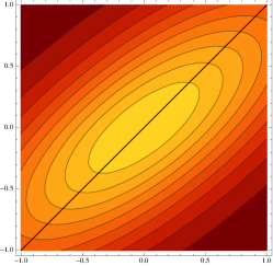
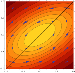
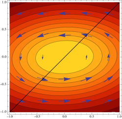
The properties of the stationary ensemble of mean and optimal trait in a fitness seascape are summarized in Fig. 2. The stationary distribution Qstat(Γ,E)subscript𝑄statΓsuperscript𝐸Q_{\rm stat}(\Gamma,E^{*}) is shown in Fig. 2(a–c) for given parameters c𝑐c, r2superscript𝑟2r^{2}, and for different values of the driving rate: in the equilibrium limit (υ0𝜐0\upsilon\to 0), for an intermediate value of υ𝜐\upsilon, and in the fast-driving regime (υr2/τeq(c)much-greater-than𝜐superscript𝑟2subscript𝜏eq𝑐\upsilon\gg r^{2}/\tau_{\rm eq}(c)). The non-equilibrium probability current 𝐉stat(Γ,E)subscript𝐉statΓsuperscript𝐸\mathbf{J}_{\rm stat}(\Gamma,E^{*}) is marked by arrows. The crossover between micro- and macro-evolutionary fitness seascapes is plotted in Fig. 2(d,e) for the scaled average square distance λ2delimited-⟨⟩superscript𝜆2\langle\lambda^{2}\rangle as a function of the driving rate υ𝜐\upsilon. Our analytical results are tested by numerical simulations of the underlying Fisher-Wright process [37] in a fitness seascape (15) with diffusive and punctuated peak displacement. The details of the numerical methods for the population simulations are discussed in Appendix B.

a b c

centered mean trait, γ^^𝛾\hat{\gamma}

Refer to caption Refer to caption Refer to caption
    centered optimal trait, e^superscript^𝑒\hat{e}^{*}     centered optimal trait, e^superscript^𝑒\hat{e}^{*}     centered optimal trait, e^superscript^𝑒\hat{e}^{*}
d e

sq. distance to peak, λ2delimited-⟨⟩superscript𝜆2{\langle}\lambda^{2}{\rangle}

Refer to caption Refer to caption
                  scaled driving rate, υ/μ𝜐𝜇\upsilon/\mu                   scaled driving rate, υ/μ𝜐𝜇\upsilon/\mu
Figure 2: Stationary distribution of mean and optimal trait in a fitness seascape. (a–c) The distribution Qstat(Γ,E)subscript𝑄statΓsuperscript𝐸Q_{\rm stat}(\Gamma,E^{*}) is shown (a) in the equilibrium limit (c=1𝑐1c=1, υ=0𝜐0\upsilon=0, r2=1superscript𝑟21r^{2}=1), (b) for an intermediate driving rate (υ=1.5r2/τeq𝜐1.5superscript𝑟2subscript𝜏eq\upsilon=1.5r^{2}/\tau_{\rm eq}), and (c) in the deep micro-evolutionary regime (υ=50r2/τeq𝜐50superscript𝑟2subscript𝜏eq\upsilon=50r^{2}/\tau_{\rm eq}); see eqs. (30), (49), and (50). The probability current 𝐉(Γ,E)𝐉Γsuperscript𝐸{\bf J}(\Gamma,E^{*}), which is given by eq. (48), is marked by arrows. With increasing driving rate, the correlation between ΓΓ\Gamma and Esuperscript𝐸E^{*} is seen to decrease. (d,e) The scaled average square distance between mean and optimal trait value, λ2delimited-⟨⟩superscript𝜆2{\langle}\lambda^{2}{\rangle}, is plotted against the scaled driving rate υ/μ𝜐𝜇\upsilon/\mu for (d) non-recombining and (e) fully recombining populations for different stabilizing strengths c𝑐c. The other parameters are r2=1superscript𝑟21r^{2}=1, θ=0.0125𝜃0.0125\theta=0.0125. This function increases from an equilibrium value for υ=0𝜐0\upsilon=0 to a micro-evolutionary limit value for υ𝜐\upsilon\to\infty with a crossover for τsat(υ,r2)τeq(c)similar-tosubscript𝜏sat𝜐superscript𝑟2subscript𝜏eq𝑐\tau_{\rm sat}(\upsilon,r^{2})\sim\tau_{\rm eq}(c), as given by eq. (43). The analytical results (lines) are compared to simulation results (with parameters N=100,=100formulae-sequence𝑁100100N=100,\ell=100) for a diffusive seascape (green dots) and for a punctuated seascape (orange dots).

3.2 Time-dependent trait divergence

In the previous paper [1], we have shown that the variance of the trait mean across populations, Γ^2delimited-⟨⟩superscript^Γ2{\langle}\hat{\Gamma}^{2}{\rangle}, and the average trait diversity Δdelimited-⟨⟩Δ{\langle}\Delta{\rangle} uniquely characterize the stabilizing strength c𝑐c in a fitness landscape. The ensemble variance Γ^2delimited-⟨⟩superscript^Γ2{\langle}\hat{\Gamma}^{2}{\rangle} is just the half of the asymptotic trait divergence limτD(τ)limτ(Γ(t+τ)Γ(t))2subscript𝜏delimited-⟨⟩𝐷𝜏subscript𝜏delimited-⟨⟩superscriptΓ𝑡𝜏Γ𝑡2\lim_{\tau\rightarrow\infty}{\langle}D(\tau){\rangle}\equiv\lim_{\tau\rightarrow\infty}{\langle}(\Gamma(t+\tau)-\Gamma(t))^{2}{\rangle}. As it is clear from the previous subsection, the stationary distribution Qstat(Γ)subscript𝑄statΓQ_{\rm stat}(\Gamma) and its statistics is compatible with different values of the seascape parameters and, hence, cannot uniquely characterize them. Instead, we will use the time-dependent average trait divergence to characterize the parameters of the fitness seascape. This quantity can be estimated between populations in one and two lineages, D(κ)(τ)delimited-⟨⟩superscript𝐷𝜅𝜏\mathcal{{\langle}}D^{(\kappa)}\rangle(\tau) (κ=1,2𝜅12\kappa=1,2), as defined in eqs. (4) and (5). The average divergence between an ancestral and a descendent population in a single lineage can be written as an expectation value in the stationary ensemble,

D(1)(τ)delimited-⟨⟩superscript𝐷1𝜏\displaystyle\langle D^{(1)}\rangle(\tau) \displaystyle\equiv (Γ(t)Γ(ta))2delimited-⟨⟩superscriptΓ𝑡Γsubscript𝑡𝑎2\displaystyle{\langle}(\Gamma(t)-\Gamma(t_{a}))^{2}{\rangle} (53)
\displaystyle\equiv dΓdΓa(ΓΓa)2×([Uncaptioned image] )dΓdsubscriptΓ𝑎superscriptΓsubscriptΓ𝑎2[Uncaptioned image] \displaystyle\int\!\text{d}\Gamma\,\text{d}\Gamma_{a}\,(\Gamma-\Gamma_{a})^{2}\,\times\left(\raisebox{-31.29802pt}{\includegraphics[height=62.59605pt]{feynman_D1} }\right)
=\displaystyle= dEadEdΓadΓ(ΓΓa)2Gτ(Γ,E|Γa,Ea)Qstat(Γa,Ea),dsubscriptsuperscript𝐸𝑎dsuperscript𝐸dsubscriptΓ𝑎dΓsuperscriptΓsubscriptΓ𝑎2subscript𝐺𝜏Γconditionalsuperscript𝐸subscriptΓ𝑎superscriptsubscript𝐸𝑎subscript𝑄statsubscriptΓ𝑎superscriptsubscript𝐸𝑎\displaystyle\int\!\text{d}E^{*}_{a}\,\text{d}E^{*}\,\text{d}\Gamma_{a}\,\text{d}\Gamma\,(\Gamma-\Gamma_{a})^{2}\,G_{\tau}(\Gamma,E^{*}\,|\,\Gamma_{a},E_{a}^{*})\,Q_{\rm stat}(\Gamma_{a},E_{a}^{*}),

where ΓaΓ(ta)subscriptΓ𝑎Γsubscript𝑡𝑎\Gamma_{a}\equiv\Gamma(t_{a}), ΓΓ(t)ΓΓ𝑡\Gamma\equiv\Gamma(t), EaE(ta)subscriptsuperscript𝐸𝑎superscript𝐸subscript𝑡𝑎E^{*}_{a}\equiv E^{*}(t_{a}), EE(t)superscript𝐸superscript𝐸𝑡E^{*}\equiv E^{*}(t), and τ=tta𝜏𝑡subscript𝑡𝑎\tau=t-t_{a}. The function Gτ(Γ,E|Γa,Ea)subscript𝐺𝜏Γconditionalsuperscript𝐸subscriptΓ𝑎superscriptsubscript𝐸𝑎G_{\tau}(\Gamma,E^{*}\,|\,\Gamma_{a},E_{a}^{*}) is the conditional probability (or propagator) for mean and optimal trait values Γ,EΓsuperscript𝐸\Gamma,E^{*} at time t𝑡t, given the values Γa,EasubscriptΓ𝑎subscriptsuperscript𝐸𝑎\Gamma_{a},E^{*}_{a} at time tasubscript𝑡𝑎t_{a}.

In a similar way, the average divergence between two descendent populations evolved from a common ancestor population is given by

D(2)(τ)delimited-⟨⟩superscript𝐷2𝜏\displaystyle{\langle}D^{(2)}{\rangle}(\tau) \displaystyle\equiv (Γ1(t)Γ2(t))2Γ1(ta)=Γ2(ta)E1(ta)=E2(ta)subscriptdelimited-⟨⟩superscriptsubscriptΓ1𝑡subscriptΓ2𝑡2subscriptΓ1subscript𝑡𝑎subscriptΓ2subscript𝑡𝑎subscriptsuperscript𝐸1subscript𝑡𝑎subscriptsuperscript𝐸2subscript𝑡𝑎\displaystyle\langle(\Gamma_{1}(t)-\Gamma_{2}(t))^{2}\rangle_{\begin{subarray}{c}\Gamma_{1}(t_{a})=\Gamma_{2}(t_{a})\\ E^{*}_{1}(t_{a})=E^{*}_{2}(t_{a})\end{subarray}} (54)
\displaystyle\equiv dΓadΓ1dΓ2(Γ1Γ2)2×([Uncaptioned image] )dsubscriptΓ𝑎dsubscriptΓ1dsubscriptΓ2superscriptsubscriptΓ1subscriptΓ22[Uncaptioned image] \displaystyle\int\!\text{d}\Gamma_{a}\,\text{d}\Gamma_{1}\,\text{d}\Gamma_{2}\,(\Gamma_{1}-\Gamma_{2})^{2}\,\times\left(\raisebox{-31.29802pt}{\includegraphics[height=62.59605pt]{feynman_D2} }\right)
=\displaystyle= dEadE1dE2dΓadΓ1dΓ2(Γ1Γ2)2Gτ/2(Γ1,E1|Γa,Ea)dsubscriptsuperscript𝐸𝑎dsubscriptsuperscript𝐸1dsubscriptsuperscript𝐸2dsubscriptΓ𝑎dsubscriptΓ1dsubscriptΓ2superscriptsubscriptΓ1subscriptΓ22subscript𝐺𝜏2subscriptΓ1conditionalsuperscriptsubscript𝐸1subscriptΓ𝑎superscriptsubscript𝐸𝑎\displaystyle\int\!\text{d}E^{*}_{a}\,\text{d}E^{*}_{1}\,\text{d}E^{*}_{2}\,\text{d}\Gamma_{a}\,\text{d}\Gamma_{1}\,\text{d}\Gamma_{2}\;(\Gamma_{1}-\Gamma_{2})^{2}\,G_{\tau/2}(\Gamma_{1},E_{1}^{*}\,|\,\Gamma_{a},E_{a}^{*})\,
×Gτ/2(Γ2,E2|Γa,Ea)Qstat(Γa,Ea),absentsubscript𝐺𝜏2subscriptΓ2conditionalsuperscriptsubscript𝐸2subscriptΓ𝑎superscriptsubscript𝐸𝑎subscript𝑄statsubscriptΓ𝑎superscriptsubscript𝐸𝑎\displaystyle\qquad\qquad\qquad\qquad\qquad\qquad\times G_{\tau/2}(\Gamma_{2},E_{2}^{*}\,|\,\Gamma_{a},E_{a}^{*})\,Q_{\rm stat}(\Gamma_{a},E_{a}^{*}),

where ΓaΓ1(ta)=Γ2(ta)subscriptΓ𝑎subscriptΓ1subscript𝑡𝑎subscriptΓ2subscript𝑡𝑎\Gamma_{a}\equiv\Gamma_{1}(t_{a})=\Gamma_{2}(t_{a}), EaE1(ta)=E2(ta)subscriptsuperscript𝐸𝑎superscriptsubscript𝐸1subscript𝑡𝑎superscriptsubscript𝐸2subscript𝑡𝑎E^{*}_{a}\equiv E_{1}^{*}(t_{a})=E_{2}^{*}(t_{a}), ΓiΓi(t)subscriptΓ𝑖subscriptΓ𝑖𝑡\Gamma_{i}\equiv\Gamma_{i}(t), EiEi(t)subscriptsuperscript𝐸𝑖subscriptsuperscript𝐸𝑖𝑡E^{*}_{i}\equiv E^{*}_{i}(t) (i=1,2𝑖12i=1,2), and τ2(tta)𝜏2𝑡subscript𝑡𝑎\tau\equiv 2(t-t_{a}). In Appendix A, we use the Langevin formalism to derive analytical expressions for these propagators and the resulting scaled divergence d(κ)(τ)D(κ)(τ)/E02,(κ=1,2)delimited-⟨⟩superscript𝑑𝜅𝜏delimited-⟨⟩superscript𝐷𝜅𝜏superscriptsubscript𝐸02𝜅12{\langle}d^{(\kappa)}\rangle(\tau)\equiv{\langle}D^{(\kappa)}\rangle(\tau)/E_{0}^{2},\;(\kappa=1,2). We obtain

d(κ)(τ;c,υ,r2)=τeq(c)τ~(c)[1eτ/τeq(c)]delimited-⟨⟩superscript𝑑𝜅𝜏𝑐𝜐superscript𝑟2subscript𝜏eq𝑐~𝜏𝑐delimited-[]1superscript𝑒𝜏subscript𝜏eq𝑐\displaystyle{\langle}d^{(\kappa)}{\rangle}(\tau;c,\upsilon,r^{2})=\frac{\tau_{\rm eq}(c)}{\tilde{\tau}(c)}\Big{[}1-e^{-\tau/\tau_{\rm eq}(c)}\Big{]} (55)
+υw(c,υ,r2)w(c,υ,r2)[τsat(v,r2)(1eτ/τsat(v,r2))τeq(c)(1eτ/τeq(c))]𝜐𝑤𝑐𝜐superscript𝑟2𝑤𝑐𝜐superscript𝑟2delimited-[]subscript𝜏sat𝑣superscript𝑟21superscripte𝜏subscript𝜏sat𝑣superscript𝑟2subscript𝜏eq𝑐1superscripte𝜏subscript𝜏eq𝑐\displaystyle+\upsilon\,w(c,\upsilon,r^{2})w(c,-\upsilon,r^{2})\left[\tau_{\rm sat}(v,r^{2})\big{(}1-{\rm e}^{-\tau/\tau_{\rm sat}(v,r^{2})}\big{)}-\tau_{\rm eq}(c)\left(1-{\rm e}^{-\tau/\tau_{\rm eq}(c)}\right)\right]
2(κ1)υτeq1(c)+τsat1(v,r2)w(c,υ,r2)2[eτ/(2τsat(v,r2))eτ/(2τeq(c))]2.2𝜅1𝜐superscriptsubscript𝜏eq1𝑐superscriptsubscript𝜏sat1𝑣superscript𝑟2𝑤superscript𝑐𝜐superscript𝑟22superscriptdelimited-[]superscripte𝜏2subscript𝜏sat𝑣superscript𝑟2superscripte𝜏2subscript𝜏eq𝑐2\displaystyle-2(\kappa-1)\frac{\upsilon}{\tau_{\rm eq}^{-1}(c)+\tau_{\rm sat}^{-1}(v,r^{2})}\,w(c,-\upsilon,r^{2})^{2}\left[{\rm e}^{-\tau/(2\tau_{\rm sat}(v,r^{2}))}-{\rm e}^{-\tau/(2\tau_{\rm eq}(c))}\right]^{2}.

The difference between the two divergence measures is a consequence of the non-equilibrium adaptive dynamics, which violate detailed balance. Equation (55) is valid for diffusive and for punctuated fitness seascapes. It contains the three characteristic time scales defined in the previous section: the drift time τ~(c)~𝜏𝑐\tilde{\tau}(c) is the scale over which the diffusion of the trait mean, in the absence of any fitness seascape, generates a trait divergence of the order of the neutral trait span E02superscriptsubscript𝐸02E_{0}^{2}; the equilibration time τeq(c)subscript𝜏eq𝑐\tau_{\rm eq}(c) governs the relaxation of the population ensemble to a mutation-selection-drift equilibrium in a fitness landscape of stabilizing strength c𝑐c; the saturation time τsatsubscript𝜏sat\tau_{\rm sat} is defined by the mean square displacement of the fitness peak reaching the driving span r2superscript𝑟2r^{2}. Here, we focus on fitness seascapes with substantial stabilizing strength and with a driving span of order of the neutral trait span (c1greater-than-or-equivalent-to𝑐1c\gtrsim 1, r21similar-tosuperscript𝑟21r^{2}\sim 1). This selection scenario is biologically relevant: it describes adaptive processes that build up large trait differences by continuous diffusion or recurrent jumps of the fitness peak.

In macro-evolutionary seascapes, the equilibration time and the non-equilibrium saturation time are well-separated, τeq(c)τsat(υ,r2\tau_{\rm eq}(c)\ll\tau_{\rm sat}(\upsilon,r^{2}). This results in three temporal regimes of the trait divergence:

  • Drift regime, ττeq(c)less-than-or-similar-to𝜏subscript𝜏eq𝑐\tau\lesssim\tau_{\rm eq}(c). The scaled divergence takes the form

    d(κ)(τ)delimited-⟨⟩superscript𝑑𝜅𝜏\displaystyle{\langle}d^{(\kappa)}{\rangle}(\tau) =\displaystyle= 2γ^2eq(1eτ/τeq)2subscriptdelimited-⟨⟩superscript^𝛾2eq1superscript𝑒𝜏subscript𝜏eq\displaystyle 2\langle\hat{\gamma}^{2}\rangle_{\rm eq}\left(1-e^{-\tau/\tau_{\rm eq}}\right) (56)
    similar-to-or-equals\displaystyle\simeq δ2Nτ(1+O(τ/τeq))(κ=1,2),delimited-⟨⟩𝛿2𝑁𝜏1𝑂𝜏subscript𝜏eq𝜅12\displaystyle\frac{\langle\delta\rangle}{2N}\,\tau\,\big{(}1+O(\tau/\tau_{\rm eq})\big{)}\qquad(\kappa=1,2),

    with an initial increase due to genetic drift and relaxation to an equilibrium value

    2γ^2eq(c)=w(c)c2subscriptdelimited-⟨⟩superscript^𝛾2eq𝑐𝑤𝑐𝑐2\langle\hat{\gamma}^{2}\rangle_{\rm eq}(c)=\frac{w(c)}{c} (57)

    due to stabilizing selection.

  • Adaptive regime, τeq(c)ττsat(v,r2)less-than-or-similar-tosubscript𝜏eq𝑐𝜏much-less-thansubscript𝜏sat𝑣superscript𝑟2\tau_{\rm eq}(c)\lesssim\tau\ll\tau_{\rm sat}(v,r^{2}). The scaled trait divergence follows

    d(κ)(τ)delimited-⟨⟩superscript𝑑𝜅𝜏\displaystyle{\langle}d^{(\kappa)}{\rangle}(\tau) =\displaystyle= [2γ^2eq(1υτ~κw(c)2)+υw(c)2τ][1+O(eτ/τeq,τ/τsat)]delimited-[]2subscriptdelimited-⟨⟩superscript^𝛾2eq1𝜐~𝜏𝜅𝑤superscript𝑐2𝜐𝑤superscript𝑐2𝜏delimited-[]1𝑂superscript𝑒𝜏subscript𝜏eq𝜏subscript𝜏sat\displaystyle\left[2\langle\hat{\gamma}^{2}\rangle_{\rm eq}\left(1-\upsilon\,\tilde{\tau}\,\kappa\,w(c)^{2}\right)+\upsilon\,w(c)^{2}\,\tau\right]\left[1+O\left(e^{-\tau/\tau_{\rm eq}},{\tau}/{\tau_{\rm sat}}\right)\right] (58)
    similar-to-or-equals\displaystyle\simeq [2γ^2eq+υ(τκτeq(c))][1+O((θc)2,eτ/τeq,τ/τsat)](κ=1,2)delimited-[]2subscriptdelimited-⟨⟩superscript^𝛾2eq𝜐𝜏𝜅subscript𝜏eq𝑐delimited-[]1𝑂superscript𝜃𝑐2superscript𝑒𝜏subscript𝜏eq𝜏subscript𝜏sat𝜅12\displaystyle\left[2\langle\hat{\gamma}^{2}\rangle_{\rm eq}+\upsilon\,(\tau-\kappa\tau_{\rm eq}(c))\right]\left[1+\;O\left((\theta c)^{2},e^{-\tau/\tau_{\rm eq}},\tau/\tau_{\rm sat}\right)\right]\;\;\;(\kappa=1,2)

    In this regime, the trait divergence is the sum of an (asymptotically constant) equilibrium component and an adaptive component, which increases with slope υ𝜐\upsilon. In a macro-evolutionary fitness seascape, this slope is, by definition, smaller than the slope in the initial drift regime (56), which allows for a clear delineation of the two regimes in empirical data. This feature will be exploited in our selection test for quantitative traits, which will be discussed in section 5.

  • Saturation regime, ττsat(v,r2)greater-than-or-equivalent-to𝜏subscript𝜏sat𝑣superscript𝑟2\tau\gtrsim\tau_{\rm sat}(v,r^{2}). On the largest time scales, the divergence

    d(κ)(τ)2γ^2eq+2r2w(c)w(c,υ,r2)(1eτ/τsat)(κ=1,2)delimited-⟨⟩superscript𝑑𝜅𝜏2subscriptdelimited-⟨⟩superscript^𝛾2eq2superscript𝑟2𝑤𝑐𝑤𝑐𝜐superscript𝑟21superscript𝑒𝜏subscript𝜏sat𝜅12{\langle}d^{(\kappa)}{\rangle}(\tau)\approx 2{\langle}\hat{\gamma}^{2}{\rangle}_{\rm eq}+2r^{2}w(c)w(c,\upsilon,r^{2})\big{(}1-e^{-\tau/\tau_{\rm sat}}\big{)}\qquad(\kappa=1,2) (59)

    approaches its non-equilibrium saturation value

    γ^2stat(c,υ,r2)=2γ^2eq+2r2w(c)w(c,υ,r2),subscriptdelimited-⟨⟩superscript^𝛾2stat𝑐𝜐superscript𝑟22subscriptdelimited-⟨⟩superscript^𝛾2eq2superscript𝑟2𝑤𝑐𝑤𝑐𝜐superscript𝑟2{\langle}\hat{\gamma}^{2}{\rangle}_{{\rm stat}}(c,\upsilon,r^{2})=2{\langle}\hat{\gamma}^{2}{\rangle}_{\rm eq}+2r^{2}w(c)w(c,\upsilon,r^{2}), (60)

    which equals the ΓΓ\Gamma-variance of the stationary distribution Qstat(Γ,E)subscript𝑄statΓsuperscript𝐸Q_{\rm stat}(\Gamma,E^{*}), and is primarily determined by the driving span r2superscript𝑟2r^{2}. In empirical data, this regime is often well beyond the depth of the phylogeny and, hence, not observable.

In micro-evolutionary seascapes, the saturation of fitness fluctuations occurs faster than the equilibration of the trait under stabilizing selection, i.e., τsat(υ,r2)τeq(c)less-than-or-similar-tosubscript𝜏sat𝜐superscript𝑟2subscript𝜏eq𝑐\tau_{\rm sat}(\upsilon,r^{2})\lesssim\tau_{\rm eq}(c). Hence, there is a direct crossover from the drift regime to the saturation regime. For fast micro-evolutionary fitness fluctuations, τsat(υ,r2)τeq(c)much-less-thansubscript𝜏sat𝜐superscript𝑟2subscript𝜏eq𝑐\tau_{\rm sat}(\upsilon,r^{2})\ll\tau_{\rm eq}(c), the constraint on the trait equals that in an effective fitness landscape with stabilizing strength ceffsubscript𝑐effc_{\rm eff} given by eq. (52). In this regime, time-dependent trait divergence data alone can no longer resolve adaptive evolution in a fitness seascape from equilibrium in the corresponding effective fitness landscape; this requires additional information on the trait diversity.

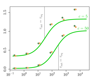
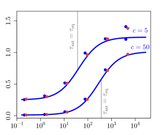
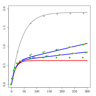
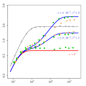
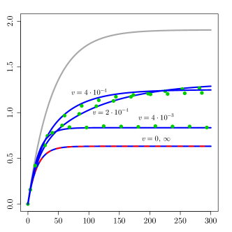
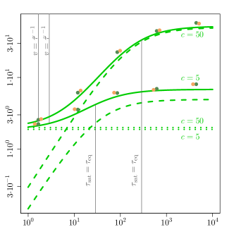
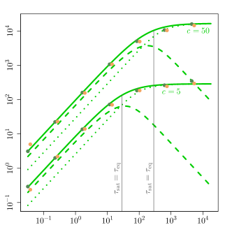
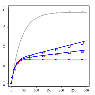
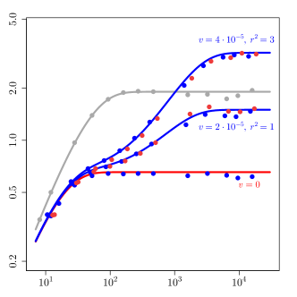
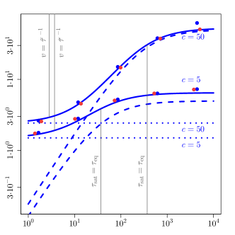
Fig. 3 and Fig. A.1(a–b) show the scaled divergence d(1)(τ)delimited-⟨⟩superscript𝑑1𝜏{\langle}d^{(1)}{\rangle}(\tau) for selection parameters c𝑐c and υ𝜐\upsilon covering macro-evolutionary and micro-evolutionary fitness seascapes. The analytical expression of eq. (55) is seen to be in good agreement with numerical simulations for diffusive and punctuated fitness fluctuations.

a b

scaled trait divergence, d(1)(τ)delimited-⟨⟩superscript𝑑1𝜏{\langle}d^{(1)}{\rangle}(\tau)

Refer to caption Refer to caption
            scaled divergence time, τ/N𝜏𝑁\tau/N             scaled divergence time, τ/N𝜏𝑁\tau/N
c

scaled trait divergence, d(1)(τ)delimited-⟨⟩superscript𝑑1𝜏{\langle}d^{(1)}{\rangle}(\tau)

Refer to caption
            scaled divergence time, τ/N𝜏𝑁\tau/N
Figure 3: Time-dependence of the trait divergence. The scaled average divergence d(1)(τ)delimited-⟨⟩superscript𝑑1𝜏\langle d^{(1)}\rangle(\tau) is shown as a function of the scaled divergence time τ/N𝜏𝑁\tau/N for three cases: neutral evolution (c=0𝑐0c=0; grey lines), conservation in a static fitness landscape (c=1𝑐1c=1, υ=0𝜐0\upsilon=0; red line), and adaptation in a macro-evolutionary fitness seascape (c=1𝑐1c=1, υ>0𝜐0\upsilon>0; blue lines). Other parameters: θ=0.0125,N=100,=100,=0.7formulae-sequence𝜃0.0125formulae-sequence𝑁100formulae-sequence1000.7\theta=0.0125,\,N=100,\,\ell=100,\,\mathcal{E}=0.7\ell. The analytical results of eq. (55) (lines) are compared to simulation results for asexual evolution in diffusive and punctuated fitness seascapes (green and orange dots, respectively). The corresponding results for fully recombining genomes are shown in Fig. A.1. (a,b) Macro-evolutionary seascapes, τsat(υ,r2)>τeq(c)subscript𝜏sat𝜐superscript𝑟2subscript𝜏eq𝑐\tau_{\rm sat}(\upsilon,r^{2})>\tau_{\rm eq}(c). (a) Linear plot: For ττeqless-than-or-similar-to𝜏subscript𝜏eq\tau\lesssim\tau_{\rm eq}, the trait evolution is dominated by genetic drift and is independent of selection. For ττeqgreater-than-or-equivalent-to𝜏subscript𝜏eq\tau\gtrsim\tau_{\rm eq}, the seascape data show an adaptive divergence component proportional to υτ𝜐𝜏\upsilon\tau; the landscape data saturate to an equilibrium divergence set by stabilizing selection. (b) Logarithmic plot: This also shows the non-equilibrium saturation of the seascape data on time scales ττsatsimilar-to𝜏subscript𝜏sat\tau\sim\tau_{\rm sat}, when the divergence reaches twice the driving span r2superscript𝑟2r^{2}. (c) Micro-evolutionary seascapes τsat(υ,r2)<τeq(c)subscript𝜏sat𝜐superscript𝑟2subscript𝜏eq𝑐\tau_{\rm sat}(\upsilon,r^{2})<\tau_{\rm eq}(c). There is a single cross-over from the drift regime for smaller values of τ𝜏\tau to the saturation regime for larger values of τ𝜏\tau. The divergence d(1)(τ)delimited-⟨⟩superscript𝑑1𝜏\langle d^{(1)}\rangle(\tau) equals that in an effective fitness landscape of stabilizing strength ceff<csubscript𝑐eff𝑐c_{\rm eff}<c. The limit υ𝜐\upsilon\to\infty has ceff=csubscript𝑐eff𝑐c_{\rm eff}=c; i.e., the function d(1)(τ)delimited-⟨⟩superscript𝑑1𝜏\langle d^{(1)}\rangle(\tau) becomes identical to the case υ=0𝜐0\upsilon=0 (blue–red dashed line).

3.3 Stationary trait diversity

As discussed in section 2, our diffusion theory predicts that the movements of the optimum trait in a single-peak fitness seascape of the form (15) only affects the evolution of the trait mean in the population and not the trait diversity. The statistics of the trait diversity remains similar to the case of evolution under stabilizing selection, which is characterized by a time-invariant fitness function, F2(Δ)=c0Δsubscript𝐹2Δsubscript𝑐0ΔF_{2}(\Delta)=-c_{0}\,\Delta. The resulting equilibrium distribution Qeq(Δ)subscript𝑄eqΔQ_{\rm eq}(\Delta) is the product of the neutral mutation-drift equilibrium Q0(Δ)subscript𝑄0ΔQ_{0}(\Delta), which is given in eqs. (53) and (55) of [1] and a Boltzmann factor from the scaled fitness landscape, Qeq(Δ)=Q0(Δ)exp[c0Δ]subscript𝑄eqΔsubscript𝑄0Δsubscript𝑐0ΔQ_{\rm eq}(\Delta)=Q_{0}(\Delta)\,\exp[-c_{0}\,\Delta]. These distributions determine the average diversity

ΔdΔΔQeq(Δ)delimited-⟨⟩ΔdΔΔsubscript𝑄eqΔ\langle\Delta\rangle\equiv\int\!\text{d}\Delta\,\Delta\,Q_{\rm eq}(\Delta) (61)

and its neutral counterpart Δ0subscriptdelimited-⟨⟩Δ0\langle\Delta\rangle_{0}, as well as the scaled expectation values δΔ/E02delimited-⟨⟩𝛿delimited-⟨⟩Δsuperscriptsubscript𝐸02\langle\delta\rangle\equiv\langle\Delta\rangle/E_{0}^{2} and δ0Δ0/E02subscriptdelimited-⟨⟩𝛿0subscriptdelimited-⟨⟩Δ0superscriptsubscript𝐸02\langle\delta\rangle_{0}\equiv\langle\Delta\rangle_{0}/E_{0}^{2}. The selective constraint on the trait diversity enters the diffusion coefficient of the trait mean in eq. (7), which sets the drift time scale τ~(c)=(1/2μ)(δ0/δ(c))~𝜏𝑐12𝜇subscriptdelimited-⟨⟩𝛿0delimited-⟨⟩𝛿𝑐\tilde{\tau}(c)=(1/2\mu)(\langle\delta\rangle_{0}/\langle\delta\rangle(c)), as given by eq. (12). The distributions Q0(Δ)subscript𝑄0ΔQ_{0}(\Delta) and Qeq(Δ)subscript𝑄eqΔQ_{\rm eq}(\Delta) can be written in closed analytical form; unlike in the case of the trait mean, these distributions depend directly on the rate of recombination in the population [1]. We obtain the scaled neutral expectation value δ0=4θ(14θ+O(θ2))subscriptdelimited-⟨⟩𝛿04𝜃14𝜃𝑂superscript𝜃2\langle\delta\rangle_{0}=4\theta(1-4\theta+O(\theta^{2})), which is independent of the recombination rate, and the selective constraint

δ(c)δ0={14θc+𝒪((θc)2) for θc1,(4θc)1/2+𝒪((θc)1) for θc1delimited-⟨⟩𝛿𝑐subscriptdelimited-⟨⟩𝛿0cases14𝜃𝑐𝒪superscript𝜃𝑐2 for θc1,superscript4𝜃𝑐12𝒪superscript𝜃𝑐1 for θc1\frac{\langle\delta\rangle(c)}{\langle\delta\rangle_{0}}=\left\{\begin{array}[]{ll}1-4\theta c+\mathcal{O}((\theta c)^{2})&\mbox{ for $\theta c\ll 1$,}\\ (4\theta c)^{-1/2}+\mathcal{O}((\theta c)^{-1})&\mbox{ for $\theta c\gg 1$}\end{array}\right. (62)

in non-recombining populations. We note that this constraint depends only on the product θc𝜃𝑐\theta c; therefore, it remains weak over a wide range of parameters (c1/θless-than-or-similar-to𝑐1𝜃c\lesssim 1/\theta), which includes strong selection effects on the trait mean [1]. The full crossover function and the corresponding expressions for fully recombining populations are given in eqs. (68) – (73) of ref. [1].

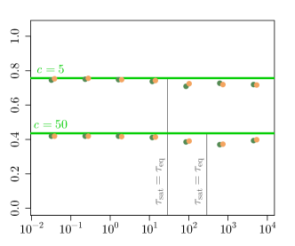
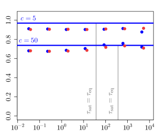
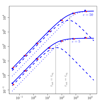
The numerical simulations reported in Fig. 4 show that the average diversity in diffusive fitness seascapes is well represented by the equilibrium value throughout the crossover from macro- to micro-evolutionary driving rates, and over a wide range of stabilizing strengths. Theoretically, the results of the diffusion theory are valid for adaptive processes unless recurrent selective sweeps reduce the trait diversity within the population. Such sweeps are more prominent in punctuated fitness seascapes due to sudden changes of the trait optimum. We expect a significant reduction in trait diversity due to the large and frequent jumps of the trait optimum in fitness seascapes with very strong stabilizing selection. This regime is beyond the scopes of this paper.

a b

scaled trait diversity, δ/δ0delimited-⟨⟩𝛿subscriptdelimited-⟨⟩𝛿0{\langle}\delta{\rangle}/{\langle}\delta{\rangle}_{0}

Refer to caption Refer to caption
                  scaled driving rate, υ/μ𝜐𝜇\upsilon/\mu                   scaled driving rate, υ/μ𝜐𝜇\upsilon/\mu
Figure 4: Stationary trait diversity. The figure shows the average trait diversity δdelimited-⟨⟩𝛿{\langle}\delta{\rangle} (in units of the neutral average δ0subscriptdelimited-⟨⟩𝛿0{\langle}\delta{\rangle}_{0}) in a fitness seascape as a function of the scaled driving rate υ/μ𝜐𝜇\upsilon/\mu for different values of the stabilizing strength (c=5,50𝑐550c=5,50, top to bottom); other parameters are as in Fig. 3. The equilibrium predictions of diffusion theory (lines), which do not depend on υ𝜐\upsilon, are compared to simulation results of the adaptive process of (a) non-recombining and (b) fully recombining populations in diffusive (green/orange dots) and punctuated seascapes (blue/red dots). The simulation results confirm evolutionary equilibrium of the trait diversity.

4 Fitness and entropy of adaptive processes

The distributions of the trait mean and diversity determine the fitness statistics of an ensemble of populations in the stationary state. These statistics can quantify the cost and the amount of adaption for the evolution of molecular traits. We also evaluate the predictability of the trait evolution in an ensemble of populations after diverging from a common ancestral population.

4.1 Genetic load

The genetic load of an individual population is defined as the difference between the maximum fitness and the mean fitness [38, 39, 40, 41],

L(t)ff¯(t).𝐿𝑡superscript𝑓¯𝑓𝑡L(t)\equiv f^{*}-\overline{f}(t). (63)

For a quantitative trait in a quadratic fitness seascape of the form (15), we can decompose the load into contributions of the trait mean and diversity,

L(t)=fc0(Γ(t)E(t))22c0Δ(t).𝐿𝑡superscript𝑓subscript𝑐0superscriptΓ𝑡superscript𝐸𝑡22subscript𝑐0Δ𝑡L(t)=f^{*}-c_{0}\big{(}\Gamma(t)-E^{*}(t)\big{)}^{2}-2c_{0}\Delta(t). (64)

In the stationary population ensemble (30), the average scaled genetic load can be written as the sum of an equilibrium and an adaptive component,

2NL(c,υ,r2)delimited-⟨⟩2𝑁𝐿𝑐𝜐superscript𝑟2\displaystyle\langle 2NL\rangle(c,\upsilon,r^{2}) =\displaystyle= c[λ2(c,υ,r2)+δ(c)]𝑐delimited-[]delimited-⟨⟩superscript𝜆2𝑐𝜐superscript𝑟2delimited-⟨⟩𝛿𝑐\displaystyle c\big{[}\langle\lambda^{2}\rangle(c,\upsilon,r^{2})+\langle\delta\rangle(c)\big{]} (65)
=\displaystyle= c[λ2eq(c,r2)+δ(c)]+c[λ2(c,υ,r2)λ2eq(c,r2)]𝑐delimited-[]subscriptdelimited-⟨⟩superscript𝜆2eq𝑐superscript𝑟2delimited-⟨⟩𝛿𝑐𝑐delimited-[]delimited-⟨⟩superscript𝜆2𝑐𝜐superscript𝑟2subscriptdelimited-⟨⟩superscript𝜆2eq𝑐superscript𝑟2\displaystyle c\big{[}\langle\lambda^{2}\rangle_{\rm eq}(c,r^{2})+\langle\delta\rangle(c)\big{]}+c\big{[}\langle\lambda^{2}\rangle(c,\upsilon,r^{2})-\langle\lambda^{2}\rangle_{\rm eq}(c,r^{2})\big{]}
\displaystyle\equiv 2NLeq(c,r2)+2NLad(c,υ,r2);2𝑁subscript𝐿eq𝑐superscript𝑟22𝑁subscript𝐿ad𝑐𝜐superscript𝑟2\displaystyle 2NL_{\rm eq}(c,r^{2})+2NL_{\rm ad}(c,\upsilon,r^{2});

these components can be computed analytically from eqs. (43) and (44). A simple form is obtained for fitness seascapes of substantial stabilizing strength (c1greater-than-or-equivalent-to𝑐1c\gtrsim 1),

2NLeq2𝑁subscript𝐿eq\displaystyle 2NL_{\rm eq} similar-to-or-equals\displaystyle\simeq 12+𝒪(1/c,θc),12𝒪1𝑐𝜃𝑐\displaystyle\frac{1}{2}+\mathcal{O}(1/c,\theta c), (66)
2NLad(c,υ,r2)2𝑁subscript𝐿ad𝑐𝜐superscript𝑟2\displaystyle 2NL_{\rm ad}(c,\upsilon,r^{2}) similar-to-or-equals\displaystyle\simeq {υτ~(c)[1+𝒪(τeqτsat)],(macroev. seascapes)cr2[1𝒪(τsatτeq)],(microev. seascapes),cases𝜐~𝜏𝑐delimited-[]1𝒪subscript𝜏eqsubscript𝜏sat(macroev. seascapes)missing-subexpressionmissing-subexpression𝑐superscript𝑟2delimited-[]1𝒪subscript𝜏satsubscript𝜏eq(microev. seascapes)\displaystyle\left\{\begin{array}[]{cc}\upsilon\,\tilde{\tau}(c)\left[1+\mathcal{O}\left(\dfrac{\tau_{\rm eq}}{\tau_{\rm sat}}\right)\right],&\mbox{(macroev. seascapes)}\\ \\ cr^{2}\Big{[}1-\mathcal{O}\Big{(}\dfrac{\tau_{\rm sat}}{\tau_{\rm eq}}\Big{)}\Big{]},&\mbox{(microev. seascapes)},\end{array}\right. (70)

where the drift scale τ~(c)~𝜏𝑐\tilde{\tau}(c) is given by eqs. (12) and (62). From these expressions, we read off three relevant properties of the genetic load.

First, the equilibrium load depends on c𝑐c only via its diversity component; this dependence remains weak even for substantial stabilizing selection (1c1/θless-than-or-similar-to1𝑐less-than-or-similar-to1𝜃1\lesssim c\lesssim 1/\theta). The equilibrium load component related to the trait mean, cλ2eq(c)𝑐subscriptdelimited-⟨⟩superscript𝜆2eq𝑐c\langle\lambda^{2}\rangle_{\rm eq}(c), becomes universal in this regime: the fluctuations of ΓΓ\Gamma are constrained to a fitness range of order 2NLeq1/2similar-to-or-equals2𝑁subscript𝐿eq122NL_{\rm eq}\simeq 1/2 around Esuperscript𝐸E^{*}, irrespectively of the stabilizing strength and the molecular details of the trait [25]. For a d𝑑d-component trait as in Fisher’s geometrical model [2], this formula generalizes to 2NLeqd/2similar-to-or-equals2𝑁subscript𝐿eq𝑑22NL_{\rm eq}\simeq d/2 [42, 43, 44]. This is a direct evolutionary analogue of the equipartition theorem in statistical thermodynamics, which states that every degree of freedom that enters the energy function quadratically contributes an average of kBT/2subscript𝑘𝐵𝑇2k_{B}T/2 to the total energy of a system at temperature T𝑇T (the proportionality factor kBsubscript𝑘𝐵k_{B} is Boltzmann’s constant). [25].

Similarly, the adaptive load component depends only weakly on c𝑐c, via the drift scale τ~(c)~𝜏𝑐\tilde{\tau}(c). At a fixed value of ΓΓ\Gamma, the stochastic displacement of the fitness peak induces a fitness cost proportional to c𝑐c; however, this effect is largely offset by an adaptive response that becomes faster with increasing c𝑐c.

Finally, the different regimes of adaptive trait evolution can be characterized in terms of the genetic load. The adaptive load is asymptotically linear in the driving rate and is subleading to the equilibrium load in the slow-driving regime (υυ~(c)1/τ~(c)less-than-or-similar-to𝜐~𝜐𝑐1~𝜏𝑐\upsilon\lesssim\tilde{\upsilon}(c)\equiv 1/\tilde{\tau}(c)). It becomes dominant for faster driving (υυ~(c)greater-than-or-equivalent-to𝜐~𝜐𝑐\upsilon\gtrsim\tilde{\upsilon}(c)) and saturates in the micro-evolutionary regime (υr2/τeq(c)greater-than-or-equivalent-to𝜐superscript𝑟2subscript𝜏eq𝑐\upsilon\gtrsim r^{2}/\tau_{\rm eq}(c)). Fig. 5(a) shows this dependence of the adaptive load on the driving rate.

a b

scaled genetic load, 2NLdelimited-⟨⟩2𝑁𝐿{\langle}2NL{\rangle}

Refer to caption

scaled fitness flux, 2Nϕ/μdelimited-⟨⟩2𝑁italic-ϕ𝜇{\langle}2N\phi{\rangle}/\mu

Refer to caption
                  scaled driving rate, υ/μ𝜐𝜇\upsilon/\mu                   scaled driving rate, υ/μ𝜐𝜇\upsilon/\mu
Figure 5: Genetic load and fitness flux. (a) Scaled genetic load 2NL2𝑁𝐿2NL (full lines) and its constituents, the adaptive genetic load, 2NLad2𝑁subscript𝐿ad2NL_{\rm ad} (dashed lines), and equilibrium genetic load, 2NLeq2𝑁subscript𝐿eq2NL_{\rm eq} (dotted lines), for stationary evolution of non-recombining populations in a fitness seascape. The load components are plotted against the scaled driving rate υ/μ𝜐𝜇\upsilon/\mu for stabilizing strengths c=5,50𝑐550c=5,50; other parameters like in Fig. 3. The analytical results of eq. (65) are compared to simulations for diffusive and punctuated fitness seascapes (green and orange dots). The corresponding data for fully recombining populations are shown in Fig. A.1. The genetic load is dominated for υ1/τ~(c)less-than-or-similar-to𝜐1~𝜏𝑐\upsilon\lesssim 1/\tilde{\tau}(c) by the equilibrium component and for υ1/τ~(c)greater-than-or-equivalent-to𝜐1~𝜏𝑐\upsilon\gtrsim 1/\tilde{\tau}(c) by the adaptive component; it saturates in the micro-evolutionary seascape regime (υr2/τeq(c)greater-than-or-equivalent-to𝜐superscript𝑟2subscript𝜏eq𝑐\upsilon\gtrsim r^{2}/\tau_{\rm eq}(c)). (b) The scaled fitness flux 2Nϕdelimited-⟨⟩2𝑁italic-ϕ\langle 2N\phi\rangle (solid line) and its components 2Nϕmacrodelimited-⟨⟩2𝑁subscriptitalic-ϕmacro{\langle}2N\phi_{\rm macro}{\rangle} and 2Nϕmicrodelimited-⟨⟩2𝑁subscriptitalic-ϕmicro{\langle}2N\phi_{\rm micro}{\rangle}, as defined in eqs. (LABEL:phimacro), are shown for the same parameters (all flux values are measured in units of 1/μ1𝜇1/\mu). In macro-evolutionary fitness seascapes, 2Nϕdelimited-⟨⟩2𝑁italic-ϕ\langle 2N\phi\rangle is an approximately linear function of the driving rate υ𝜐\upsilon and the component 2Nϕmacrodelimited-⟨⟩2𝑁subscriptitalic-ϕmacro{\langle}2N\phi_{\rm macro}{\rangle} is the dominant part. In micro-evolutionary seascapes, 2Nϕdelimited-⟨⟩2𝑁italic-ϕ\langle 2N\phi\rangle saturates and the component 2Nϕmicrodelimited-⟨⟩2𝑁subscriptitalic-ϕmicro{\langle}2N\phi_{\rm micro}{\rangle} is the dominant part.

4.2 Fitness flux

The fitness flux, ϕ(t)italic-ϕ𝑡\phi(t), characterizes the adaptive response of a population evolving in a fitness land- or seascape,

ϕ(t)=dEf(E,t)t𝒲(E,t).italic-ϕ𝑡d𝐸𝑓𝐸𝑡𝑡𝒲𝐸𝑡\phi(t)=\int\!\text{d}E\,f(E,t)\,\frac{\partial}{\partial t}\mathcal{W}(E,t). (71)

The cumulative fitness flux, Φ(τ)=tt+τϕ(t)𝑑tΦ𝜏superscriptsubscript𝑡𝑡𝜏italic-ϕsuperscript𝑡differential-dsuperscript𝑡\Phi(\tau)=\int_{t}^{t+\tau}\phi(t^{\prime})dt^{\prime}, measures the total amount of adaptation over an evolutionary period τ𝜏\tau [45]. The evolutionary statistics of this quantity is specified by the fitness flux theorem [17]. According to the theorem, the average cumulative fitness flux in a population ensemble measures the deviation of the evolutionary process from equilibrium: this deviation equals the relative entropy of the actual process from a hypothetical time-reversed process [17, 46]. It is substantial — i.e., the process is predominantly adaptive — if 2NΦ1greater-than-or-equivalent-todelimited-⟨⟩2𝑁Φ1\langle 2N\Phi\rangle\gtrsim 1. Specifically, the cumulative fitness flux of a stationary adaptive process increases linearly with time, 2NΦ(τ)=ϕτdelimited-⟨⟩2𝑁Φ𝜏delimited-⟨⟩italic-ϕ𝜏\langle 2N\Phi(\tau)\rangle=\langle\phi\rangle\tau with ϕ>0delimited-⟨⟩italic-ϕ0\langle\phi\rangle>0.

For a quantitative trait in a quadratic fitness seascape of the form (15), we can decompose the fitness flux into contributions of the trait mean and the trait diversity,

ϕ(t)=2c0(Γ(t)E(t))dΓ(t)dt2c0dΔ(t)dt.italic-ϕ𝑡2subscript𝑐0Γ𝑡superscript𝐸𝑡dΓ𝑡d𝑡2subscript𝑐0dΔ𝑡d𝑡\phi(t)=-2c_{0}\big{(}\Gamma(t)-E^{*}(t)\big{)}\frac{\text{d}\Gamma(t)}{\text{d}t}-2c_{0}\frac{\text{d}\Delta(t)}{\text{d}t}. (72)

In the stationary population ensemble (30), the average scaled fitness flux can be expressed in terms of the stationary probability current 𝐉stat(Γ,E)subscript𝐉statΓsuperscript𝐸{\mathbf{J}}_{\rm stat}(\Gamma,E^{*}),

2Nϕ=2cE02dΓdE(ΓE)JstatΓ(Γ,E),delimited-⟨⟩2𝑁italic-ϕ2𝑐superscriptsubscript𝐸02dΓdsuperscript𝐸Γsuperscript𝐸superscriptsubscript𝐽statΓΓsuperscript𝐸\langle 2N\phi\rangle=-\frac{2c}{E_{0}^{2}}\int\!\text{d}\Gamma\text{d}E^{*}\,(\Gamma-E^{*})J_{\rm stat}^{\Gamma}(\Gamma,E^{*}), (73)

where JstatΓ(Γ,E)superscriptsubscript𝐽statΓΓsuperscript𝐸J_{\rm stat}^{\Gamma}(\Gamma,E^{*}) is the ΓΓ\Gamma–component of 𝐉stat(Γ,E)subscript𝐉statΓsuperscript𝐸{\mathbf{J}}_{\rm stat}(\Gamma,E^{*}). The fitness flux can be computed analytically from eq. (48),

2Nϕ(c,υ,r2)=2cυw(c,υ,r2).delimited-⟨⟩2𝑁italic-ϕ𝑐𝜐superscript𝑟22𝑐𝜐𝑤𝑐𝜐superscript𝑟2\langle 2N\phi\rangle(c,\upsilon,r^{2})=2c\upsilon\,w(c,\upsilon,r^{2}). (74)

In the regime of substantial stabilizing strength (c1greater-than-or-equivalent-to𝑐1c\gtrsim 1), we get

2Nϕ(c,υ,r2){2cυ[1𝒪(τeqτsat)](macroev. seascapes),4c2r2τ~(c)[1𝒪(τsatτeq)](microev. seascapes),similar-to-or-equalsdelimited-⟨⟩2𝑁italic-ϕ𝑐𝜐superscript𝑟2cases2𝑐𝜐delimited-[]1𝒪subscript𝜏eqsubscript𝜏sat(macroev. seascapes)missing-subexpressionmissing-subexpression4superscript𝑐2superscript𝑟2~𝜏𝑐delimited-[]1𝒪subscript𝜏satsubscript𝜏eq(microev. seascapes)\langle 2N\phi\rangle(c,\upsilon,r^{2})\simeq\left\{\begin{array}[]{cc}2c\upsilon\Big{[}1-\mathcal{O}\Big{(}\dfrac{\tau_{\rm eq}}{\tau_{\rm sat}}\Big{)}\Big{]}&\mbox{(macroev. seascapes)},\\ \\ \dfrac{4c^{2}r^{2}}{\tilde{\tau}(c)}\,\Big{[}1-\mathcal{O}\Big{(}\dfrac{\tau_{\rm sat}}{\tau_{\rm eq}}\Big{)}\Big{]}&\mbox{(microev. seascapes)},\end{array}\right. (75)

where the drift time τ~(c)~𝜏𝑐\tilde{\tau}(c) is given by eqs. (12) and (62). The fitness flux depends linearly on the driving rate in a macro-evolutionary fitness seascape, and it saturates in the regime of micro-evolutionary fitness fluctuations. Fig. 5(b) shows this dependence of the fitness flux on the driving rate.

We can express the fitness flux in terms of correlation functions of the trait mean Γ(t)Γ𝑡\Gamma(t) and the lag Λ(t)Λ𝑡\Lambda(t), which results in a simple relation between fitness flux and adaptive load. Inserting the probability current of eq. (48) into the integral of eq. (73), we find

2Nϕdelimited-⟨⟩2𝑁italic-ϕ\displaystyle{\langle}2N\phi{\rangle} =\displaystyle= 2c2δE02(Λ2Λ2eq)+4cθE02limτ0(Λ(t+τ)(Γ(t)Γ0)Λ(t+τ)(Γ(t)Γ0)eq)2superscript𝑐2delimited-⟨⟩𝛿superscriptsubscript𝐸02delimited-⟨⟩superscriptΛ2subscriptdelimited-⟨⟩superscriptΛ2eq4𝑐𝜃superscriptsubscript𝐸02subscript𝜏0delimited-⟨⟩Λ𝑡𝜏Γ𝑡subscriptΓ0subscriptdelimited-⟨⟩Λ𝑡𝜏Γ𝑡subscriptΓ0eq\displaystyle\frac{2c^{2}{\langle}\delta{\rangle}}{E_{0}^{2}}\Big{(}{\langle}\Lambda^{2}{\rangle}-{\langle}\Lambda^{2}{\rangle}_{\rm eq}\Big{)}+\frac{4c\theta}{E_{0}^{2}}\lim_{\tau\searrow 0}\Big{(}{\langle}\Lambda(t+\tau)(\Gamma(t)-\Gamma_{0}){\rangle}-{\langle}\Lambda(t+\tau)(\Gamma(t)-\Gamma_{0}){\rangle}_{\rm eq}\Big{)} (76)
=\displaystyle= cδ2NLad(c,v,r2)[1+𝒪(θ)].𝑐delimited-⟨⟩𝛿subscriptdelimited-⟨⟩2𝑁𝐿ad𝑐𝑣superscript𝑟2delimited-[]1𝒪𝜃\displaystyle c{\langle}\delta{\rangle}{\langle}2NL{\rangle}_{\rm ad}(c,v,r^{2})[1+\mathcal{O}(\theta)].

From this representation, we obtain the spectral decomposition of the fitness flux,

2Nϕ(c,υ,r2)=02Nϕ(ω)𝑑ωdelimited-⟨⟩2𝑁italic-ϕ𝑐𝜐superscript𝑟2superscriptsubscript0delimited-⟨⟩2𝑁italic-ϕ𝜔differential-d𝜔\langle 2N\phi\rangle(c,\upsilon,r^{2})=\int_{0}^{\infty}\langle 2N\phi(\omega)\rangle\,d\omega (77)

with

2Nϕ(ω)delimited-⟨⟩2𝑁italic-ϕ𝜔\displaystyle\langle 2N\phi(\omega)\rangle =\displaystyle= 2cυcδπ/2ω2(τeq2(c)+ω2)(τsat2(v,r2)+ω2)[1+𝒪(θ/(cδ)].\displaystyle 2c\upsilon\frac{c{\langle}\delta{\rangle}}{{\pi/2}}\frac{\omega^{2}}{(\tau_{\rm eq}^{-2}(c)+\omega^{2})(\tau_{\rm sat}^{-2}(v,r^{2})+\omega^{2})}[1+\mathcal{O}(\theta/(c{\langle}\delta{\rangle})]. (78)

Using a cutoff frequency ωc=k/τeq(c)subscript𝜔𝑐𝑘subscript𝜏eq𝑐\omega_{c}=k/\tau_{\rm eq}(c) with a constant k𝑘k of order 1, we can now define a macro-evolutionary flux component,

2Nϕmacrodelimited-⟨⟩2𝑁subscriptitalic-ϕmacro\displaystyle\langle 2N\phi_{\rm macro}\rangle =\displaystyle= 0ωc2Nϕ(ω)𝑑ωsuperscriptsubscript0subscript𝜔𝑐delimited-⟨⟩2𝑁italic-ϕ𝜔differential-d𝜔\displaystyle\int_{0}^{\omega_{c}}\langle 2N\phi(\omega)\rangle\,d\omega
=\displaystyle= 2cυw(c,υ,r2)(τeq1(c)+2μ)arctan[k](τsat1(υ,r2)+2μ)arctan[kτsat(v,r2)/τeq(c)](π/2)(τeq1(c)τsat1(υ,r2)),2𝑐𝜐𝑤𝑐𝜐superscript𝑟2superscriptsubscript𝜏eq1𝑐2𝜇𝑘superscriptsubscript𝜏sat1𝜐superscript𝑟22𝜇𝑘subscript𝜏sat𝑣superscript𝑟2subscript𝜏eq𝑐𝜋2superscriptsubscript𝜏eq1𝑐superscriptsubscript𝜏sat1𝜐superscript𝑟2\displaystyle 2c\upsilon\;w(c,\upsilon,r^{2})\frac{({\tau_{\rm eq}^{-1}(c)+2\mu})\arctan[k]-({\tau_{\rm sat}^{-1}(\upsilon,r^{2})+2\mu})\arctan\left[k\,\tau_{\rm sat}(v,r^{2})/\tau_{\rm eq}(c)\right]}{(\pi/2)(\tau_{\rm eq}^{-1}(c)-\tau_{\rm sat}^{-1}(\upsilon,r^{2}))},

and the complementary micro-evolutionary component

2Nϕmicro=ωc2Nϕ(ω)𝑑ω=2Nϕ2Nϕmacro.delimited-⟨⟩2𝑁subscriptitalic-ϕmicrosuperscriptsubscriptsubscript𝜔𝑐delimited-⟨⟩2𝑁italic-ϕ𝜔differential-d𝜔delimited-⟨⟩2𝑁italic-ϕdelimited-⟨⟩2𝑁subscriptitalic-ϕmacro\displaystyle\langle 2N\phi_{\rm micro}\rangle=\int_{\omega_{c}}^{\infty}\langle 2N\phi(\omega)\rangle\,d\omega=\langle 2N\phi\rangle-\langle 2N\phi_{\rm macro}\rangle. (80)

In the regime of substantial stabilizing selection (c1greater-than-or-equivalent-to𝑐1c\gtrsim 1), the macro-evolutionary fitness flux in (LABEL:phimacro) reads

2Nϕmacro(c,υ,r2)delimited-⟨⟩2𝑁subscriptitalic-ϕmacro𝑐𝜐superscript𝑟2\displaystyle\langle 2N\phi_{\rm macro}\rangle(c,\upsilon,r^{2}) similar-to-or-equals\displaystyle\simeq {2cυ2πarctan[k],(macroev. seascapes)2cυτsat2(υ,r2)τeq2(c)2π(karctan[k])1v(microev. seascapes).cases2𝑐𝜐2𝜋𝑘(macroev. seascapes)otherwiseotherwisesimilar-to2𝑐𝜐superscriptsubscript𝜏sat2𝜐superscript𝑟2superscriptsubscript𝜏eq2𝑐2𝜋𝑘𝑘1𝑣(microev. seascapes)\displaystyle\begin{cases}2c\upsilon\,\dfrac{2}{\pi}\arctan[k],&\mbox{(macroev. seascapes)}\\ \\ 2c\upsilon\,\dfrac{\tau_{\rm sat}^{2}(\upsilon,r^{2})}{\tau_{\rm eq}^{2}(c)}\,\dfrac{2}{\pi}\big{(}k-\arctan[k]\big{)}\sim\dfrac{1}{v}&\mbox{(microev. seascapes)}.\end{cases} (81)

This fitness flux component quantifies the macro-evolutionary part of adaptation. In macro-evolutionary fitness seascapes (τsat(υ,r2)τeq(c)greater-than-or-equivalent-tosubscript𝜏sat𝜐superscript𝑟2subscript𝜏eq𝑐\tau_{\rm sat}(\upsilon,r^{2})\gtrsim\tau_{\rm eq}(c)), it increases proportionally to the driving rate υ𝜐\upsilon and, for k>1𝑘1k>1, it represents the main fraction of the total fitness flux 2Nϕdelimited-⟨⟩2𝑁italic-ϕ{\langle}2N\phi{\rangle}. In micro-evolutionary fitness seascapes (τsat(υ,r2)τeq(c)less-than-or-similar-tosubscript𝜏sat𝜐superscript𝑟2subscript𝜏eq𝑐\tau_{\rm sat}(\upsilon,r^{2})\lesssim\tau_{\rm eq}(c)), this component is suppressed: the macro-evolutionary fitness flux does not carry information on rapid fitness fluctuations. This cross-over of 2Nϕmacrodelimited-⟨⟩2𝑁subscriptitalic-ϕmacro\langle 2N\phi_{\rm macro}\rangle and of the complementary component 2Nϕmicrodelimited-⟨⟩2𝑁subscriptitalic-ϕmicro\langle 2N\phi_{\rm micro}\rangle is shown in Fig. 5(b).

The spectral decomposition of the fitness flux has important consequences for the analysis of macro-evolutionary adaptation. The detection of a substantial cumulative fitness flux 2NΦmacro(τ)>1delimited-⟨⟩2𝑁subscriptΦmacro𝜏1\langle 2N\Phi_{\rm macro}(\tau)\rangle>1 over a macro-evolutionary period τ𝜏\tau is not confounded by the simultaneous presence of micro-evolutionary (for example seasonal) fitness fluctuations. Since the cumulative fitness flux is a measure of entropy production during adaptation, the spectral decomposition (77) also has an important information-theoretic interpretation: The difference 2Nϕmicro=2Nϕ2Nϕmacrodelimited-⟨⟩2𝑁subscriptitalic-ϕmicrodelimited-⟨⟩2𝑁italic-ϕdelimited-⟨⟩2𝑁subscriptitalic-ϕmacro\langle 2N\phi_{\rm micro}\rangle=\langle 2N\phi\rangle-\langle 2N\phi_{\rm macro}\rangle is the average loss of information per unit time through temporal coarse-graining. This loss is a non-equilibrium analogue of the entropy production by spatial coarse-graining.

4.3 Predictability and entropy production

In ref. [1], we quantified the evolutionary predictability of the molecular traits across an ensemble of populations by

𝒫exp[S(𝒲)S(W)],𝒫delimited-⟨⟩𝑆𝒲𝑆delimited-⟨⟩𝑊\mathcal{P}\equiv\exp\big{[}\langle{S({\cal W})}\rangle-S(\langle W\rangle)\big{]}, (82)

with S(𝒲)𝒲(E)log𝒲(E)𝑑E𝑆𝒲𝒲𝐸𝒲𝐸differential-d𝐸S({\cal W})\equiv-\int{\cal W}(E)\,\log{\cal W}(E)dE. This definition compares the ensemble-averaged “micro-evolutionary” Shannon entropy of the phenotype distribution within a population, S(𝒲)𝒲S(𝒲)Q(𝒲),delimited-⟨⟩𝑆𝒲subscript𝒲𝑆𝒲𝑄𝒲\langle S{({\cal W})}\rangle\equiv\int_{{\cal W}}S({\cal W})\,Q({\cal W}), and the “macro-evolutionary” Shannon entropy of the mixed distribution, S(𝒲)S(𝒲𝒲Q(𝒲)),𝑆delimited-⟨⟩𝒲𝑆subscript𝒲𝒲𝑄𝒲S(\langle{\cal W}\rangle)\equiv S\big{(}\int_{{\cal W}}{\cal W}\,Q({\cal W})\big{)}, which is obtained by compounding the trait values of all populations into a single distribution. We have shown that the predictability is generically low in a neutral ensemble, but stabilizing selection in a single fitness landscape can generate an evolutionary equilibrium wiht predictability values 𝒫𝒫\mathcal{P} of order 1 [1].

Here we compute the predictability in a time-dependent ensemble of populations that descend from a common ancestor population. Similarly to ref. [1], we evaluate eq. (82) for a distribution Qt(𝒲)subscript𝑄𝑡𝒲Q_{t}({\cal W}) with the initial condition Qta(𝒲)=δ(𝒲𝒲a)subscript𝑄subscript𝑡𝑎𝒲𝛿𝒲subscript𝒲𝑎Q_{t_{a}}({\cal W})=\delta({\cal W}-{\cal W}_{a}) at time ta=tτ/2subscript𝑡𝑎𝑡𝜏2t_{a}=t-\tau/2. We obtain the time-dependent predictability

𝒫(τ;c,υ,r2)(δ(c)d(2)(τ;c,υ,r2)/2+δ(c))1/2=(11+Ω(2)(τ;c,υ,r2)/4θ)1/2.similar-to-or-equals𝒫𝜏𝑐𝜐superscript𝑟2superscriptdelimited-⟨⟩𝛿𝑐delimited-⟨⟩superscript𝑑2𝜏𝑐𝜐superscript𝑟22delimited-⟨⟩𝛿𝑐12superscript11superscriptΩ2𝜏𝑐𝜐superscript𝑟24𝜃12\mathcal{P}(\tau;c,\upsilon,r^{2})\simeq\left(\frac{\langle\delta\rangle(c)}{\langle d^{(2)}\rangle(\tau;c,\upsilon,r^{2})/2+\langle\delta\rangle(c)}\right)^{1/2}=\left(\frac{1}{1+\Omega^{(2)}(\tau;c,\upsilon,r^{2})/4\theta}\right)^{1/2}. (83)

Here, Ω(2)(τ;c,v,r2)2θd(2)(τ;c,υ,r2)/δsuperscriptΩ2𝜏𝑐𝑣superscript𝑟22𝜃delimited-⟨⟩superscript𝑑2𝜏𝑐𝜐superscript𝑟2delimited-⟨⟩𝛿\Omega^{(2)}(\tau;c,v,r^{2})\equiv 2\theta\,\langle d^{(2)}\rangle(\tau;c,\upsilon,r^{2})/\langle\delta\rangle denotes the ratio between trait divergence and diversity for the descendent populations. The trait statistics in a macro-evolutionary fitness seascape, given by eqs. (55) and (62), entail the evolutionary predictability

𝒫(τ;c,υ,r2)𝒫𝜏𝑐𝜐superscript𝑟2\displaystyle\mathcal{P}(\tau;c,\upsilon,r^{2}) =\displaystyle= 𝒫eq(c)[112υτ~τ2τeq(c)2N[1+𝒪(ττeq(c)cv/N,τ/τsat,θ/(cδ))]]subscript𝒫eq𝑐delimited-[]112𝜐~𝜏𝜏2subscript𝜏eq𝑐2𝑁delimited-[]1𝒪𝜏subscript𝜏eq𝑐𝑐𝑣𝑁𝜏subscript𝜏sat𝜃𝑐delimited-⟨⟩𝛿\displaystyle\mathcal{P}_{\rm eq}(c)\left[1-\frac{1}{2}\upsilon\,\tilde{\tau}\frac{\tau-2\tau_{\rm eq}(c)}{2N}\,\Big{[}1+\mathcal{O}\left(\tau\,\tau_{\rm eq}(c)cv/N,\tau/\tau_{\rm sat},\theta/(c{\langle}\delta{\rangle})\right)\Big{]}\right] (84)

for ττeq(c)greater-than-or-equivalent-to𝜏subscript𝜏eq𝑐\tau\gtrsim\tau_{\rm eq}(c), with 𝒫eq(c)=(1+w(c)/(2c))1/2=(1+1/(2c))1/2[1+𝒪(θ/(cδ))]subscript𝒫eq𝑐superscript1𝑤𝑐2𝑐12superscript112𝑐12delimited-[]1𝒪𝜃𝑐delimited-⟨⟩𝛿\mathcal{P}_{\rm eq}(c)=(1+w(c)/(2c))^{-1/2}=(1+1/(2c))^{-1/2}[1+\mathcal{O}(\theta/(c{\langle}\delta{\rangle}))]. There are two stochastic components that generate macro-evolutionary entropy and, hence, reduce the evolutionary predictability: fluctuations induced by genetic drift on short time-scales ττeq(c)less-than-or-similar-to𝜏subscript𝜏eq𝑐\tau\lesssim\tau_{\rm eq}(c) and fluctuations of the fitness peak over time-scales ττeq(c)greater-than-or-equivalent-to𝜏subscript𝜏eq𝑐\tau\gtrsim\tau_{\rm eq}(c). Stabilizing selection, on the other hand, reduces the entropy production of the adaptive process [25]. Therefore, the predictability of an adaptive process in a fitness seascape with a substantial stabilizing strength and sufficiently slow driving rate can remain of order one.

Parallel and convergent evolution at the functional level, paired with strongly divergent genome evolution has been observed in a number of recent experiments [47, 48, 49]. These experimental observations can be explained in a natural way, if we assume that many of these functions involve a complex quantitative trait.

5 Inference of adaptive trait evolution

The statistical theory developed in this paper suggests a new method to infer selection on quantitative traits. Our method is based on trait evolution in a single-peak fitness seascape, as defined in eq. (15), which is parametrized by its stabilizing strength c𝑐c and its driving rate υ𝜐\upsilon.

Two main results are relevant for the inference of selection. First, evolution in a macro-evolutionary fitness seascape affects the population mean trait in complementary ways: it generates conservation on shorter scales and adaptation on longer scales of evolutionary time. These characteristics are measured by the expected trait divergence between populations, D(κ)(τ)delimited-⟨⟩superscript𝐷𝜅𝜏\langle D^{(\kappa)}(\tau)\rangle, which depends on the divergence time τ𝜏\tau and on the selection parameters c𝑐c and υ𝜐\upsilon in a characteristic way. The divergence can be measured either between an ancestral population and a descendent population (κ=1𝜅1\kappa=1) or between two descendent populations evolving from a common ancestor population (κ=2𝜅2\kappa=2). As discussed in section 3.2, these measures are generically distinct for adaptive processes222The relative difference between D(1)(τ)delimited-⟨⟩superscript𝐷1𝜏\langle D^{(1)}(\tau)\rangle and D(2)(τ)delimited-⟨⟩superscript𝐷2𝜏\langle D^{(2)}(\tau)\rangle is small (Fig. 5). This difference is conceptually important, however, because it manifests the violation of detailed balance in adaptive processes. Similar effects are ubiquitous in divergence data of trait adaptation across multi-branch phylogenies.. Second, the expected trait diversity within populations, Δdelimited-⟨⟩Δ\langle\Delta\rangle, shows a weaker signal of conservation. Moreover, it decouples from the adaptive process in a single-peak fitness seascape over a wide range of evolutionary parameters, as discussed in section 3.3.

Our test statistics is the time-dependent divergence-diversity ratio

Ω(κ)(τ)=2θD(κ)(τ)Δ(κ=1,2),superscriptΩ𝜅𝜏2𝜃delimited-⟨⟩superscript𝐷𝜅𝜏delimited-⟨⟩Δ𝜅12\Omega^{(\kappa)}(\tau)=2\theta\frac{\langle D^{(\kappa)}(\tau)\rangle}{\langle\Delta\rangle}\qquad(\kappa=1,2), (85)

where θ=μN𝜃𝜇𝑁\theta=\mu N denotes the nucleotide diversity. This function depends on the divergence time τ𝜏\tau and on the selection parameters c𝑐c and υ𝜐\upsilon. The typical behavior of Ω(κ)(τ)superscriptΩ𝜅𝜏\Omega^{(\kappa)}(\tau) for different evolutionary modes is shown in Fig. 6 and can be summarized as follows:

  • Neutral evolution (c=0𝑐0c=0). The divergence-diversity ratio has an initially linear increase due to genetic drift and approaches a maximum value 1 with a relaxation time τ0=1/μsubscript𝜏01𝜇\tau_{0}=1/\mu,

    Ω(κ)(τ)superscriptΩ𝜅𝜏\displaystyle\Omega^{(\kappa)}(\tau) =\displaystyle= Ω0(τ){μτ for ττ01 for ττ0(κ=1,2).similar-to-or-equalssubscriptΩ0𝜏cases𝜇𝜏 for ττ01 for ττ0𝜅12\displaystyle\Omega_{0}(\tau)\simeq\left\{\begin{array}[]{ll}\mu\tau&\mbox{ for $\tau\ll\tau_{0}$}\\ 1&\mbox{ for $\tau\gg\tau_{0}$}\end{array}\right.\qquad(\kappa=1,2). (88)

    The function Ω0(τ)subscriptΩ0𝜏\Omega_{0}(\tau), which does not depend on κ𝜅\kappa by detailed balance, is shown as a grey line in Fig. 6.

  • Conservation in a fitness landscape (c1,υ=0formulae-sequencegreater-than-or-equivalent-to𝑐1𝜐0c\gtrsim 1,\upsilon=0). The divergence-diversity ratio approaches a smaller maximum value, Ωstab(c)<1subscriptΩstab𝑐1\Omega_{\rm stab}(c)<1, with a proportionally shorter relaxation time τeq(c)=Ωstab(c)/μsubscript𝜏eq𝑐subscriptΩstab𝑐𝜇\tau_{\rm eq}(c)=\Omega_{\rm stab}(c)/\mu,

    Ω(κ)(τ)superscriptΩ𝜅𝜏\displaystyle\Omega^{(\kappa)}(\tau) =\displaystyle= Ωeq(τ;c){μτ for ττeq(c)Ωstab(c) for ττeq(c)(κ=1,2).similar-to-or-equalssubscriptΩeq𝜏𝑐cases𝜇𝜏 for ττeq(c)subscriptΩstab𝑐 for ττeq(c)𝜅12\displaystyle\Omega_{\rm eq}(\tau;c)\simeq\left\{\begin{array}[]{ll}\mu\tau&\mbox{ for $\tau\ll\tau_{\rm eq}(c)$}\\ \Omega_{\rm stab}(c)&\mbox{ for $\tau\gg\tau_{\rm eq}(c)$}\end{array}\right.\qquad(\kappa=1,2). (91)

    The function Ωeq(τ;c)subscriptΩeq𝜏𝑐\Omega_{\rm eq}(\tau;c), which does not depend on κ𝜅\kappa by detailed balance, is shown as a red line in Fig. 6. Over a wide range of evolutionary parameters, the maximum value depends on the stabilizing strength in a simple way, Ωstab(c)1/(2c)similar-tosubscriptΩstab𝑐12𝑐\Omega_{\rm stab}(c)\sim 1/(2c), with corrections for weaker selection and for larger nucleotide diversity.

  • Adaptation in a macro-evolutionary fitness seascape (c1,0<υ1/τ~formulae-sequencegreater-than-or-equivalent-to𝑐10𝜐less-than-or-similar-to1~𝜏c\gtrsim 1,0<\upsilon\lesssim 1/\tilde{\tau}). The divergence-diversity ratio acquires an adaptive component,

    Ω(κ)(τ)superscriptΩ𝜅𝜏\displaystyle\Omega^{(\kappa)}(\tau) =\displaystyle= Ωeq(τ;c)+Ωad(κ)(τ;υ)subscriptΩeq𝜏𝑐superscriptsubscriptΩad𝜅𝜏𝜐\displaystyle\Omega_{\rm eq}(\tau;c)+\Omega_{\rm ad}^{(\kappa)}(\tau;\upsilon) (92)
    =\displaystyle= Ωeq(τ;c)+υ2[τκτeq(c)](κ=1,2),subscriptΩeq𝜏𝑐𝜐2delimited-[]𝜏𝜅subscript𝜏eq𝑐𝜅12\displaystyle\Omega_{\rm eq}(\tau;c)+\frac{\upsilon}{2}\,[\tau-\kappa\tau_{\rm eq}(c)]\qquad(\kappa=1,2),

    with corrections for weaker selection and for τ𝜏\tau approaching the non-equilibrium saturation time τsat=r2/υsubscript𝜏satsuperscript𝑟2𝜐\tau_{\rm sat}=r^{2}/\upsilon. The functions Ω(κ)(τ)superscriptΩ𝜅𝜏\Omega^{(\kappa)}(\tau) are shown as blue lines in Fig. 6.

The ΩΩ\Omega-test for selection on quantitative traits is conceptually related to the McDonald-Kreitman test for adaptive sequence evolution [50]; both tests are based on a comparison between divergence and diversity. However, the ΩΩ\Omega statistics does not require a corresponding “null trait” that evolves near neutrality and takes the role of synonymous sequences. Indeed, no such neutral trait gauge is available in most cases. The ΩΩ\Omega-test instead evaluates time-resolved divergence data D(τ)𝐷𝜏D(\tau). In macro-evolutionary fitness seascapes, this test infers stabilizing and directional selection using their different characteristic time scales. In principle, a single data point in the saturation regime ττeq(c)greater-than-or-equivalent-to𝜏subscript𝜏eq𝑐\tau\gtrsim\tau_{\rm eq}(c) determines the stabilizing strength of a fitness landscape, and two data points are sufficient to determine strength and driving rate of a fitness seascape. Our statistical theory also specifies an error model for the probabilistic inference of seascape parameters from noisy data, based on the statistics of the finite time propagator detailed in Appendix A. This inference method can be generalized from single lineages to multi-species phylogenies and will be discussed in a forthcoming empirical study.

An important prerequisite for the wide applicability of the ΩΩ\Omega test is its universality: the divergence-diversity ratio depends on the selection parameters c𝑐c and υ𝜐\upsilon, but it decouples from the trait’s genetic basis. In particular, it depends only weakly on the number and trait amplitudes of the constitutive sequence sites, and on the amount of recombination between these sites. All of these genetic factors are, in general, unknown. They act as confounding factors on non-universal observables such as the trait divergence and diversity, which have been used in previous studies to infer selection [18, 16]. The ΩΩ\Omega statistics also decouples from details of the selection dynamics; it can be applied to continual as well as to punctuated adaptive processes. We have tested this universality by extensive numerical simulations, which are reported in Appendix B.
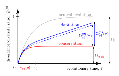
Refer to caption

Figure 6: The universal divergence-diversity ratio Ω(κ)superscriptΩ𝜅\Omega^{(\kappa)} (κ=1,2𝜅12\kappa=1,2), as defined in eq. (85), for a quantitative trait evolving in a single-peak fitness land- or seascape. This ratio is plotted as a function of the scaled divergence time, τ𝜏\tau. Neutral evolution: The function Ω0(τ)subscriptΩ0𝜏\Omega_{0}(\tau) is independent of κ𝜅\kappa and reaches its saturation value 1 on times scales ττ0=1/μmuch-greater-than𝜏subscript𝜏01𝜇\tau\gg\tau_{0}=1/\mu (grey curve). Conservation in a fitness landscape: The function Ωeq(τ)subscriptΩeq𝜏\Omega_{\rm eq}(\tau) is independent of κ𝜅\kappa and has a smaller saturation value Ωstab(c)subscriptΩstab𝑐\Omega_{\rm stab}(c) reached faster than for neutral evolution, on time scales ττeq(c)much-greater-than𝜏subscript𝜏eq𝑐\tau\gg\tau_{\rm eq}(c) (red curve). Adaptation in a fitness seascape: There is a linear surplus Ωad(κ)(τ)υ[τκτeq(c)]similar-to-or-equalssuperscriptsubscriptΩad𝜅𝜏𝜐delimited-[]𝜏𝜅subscript𝜏eq𝑐\Omega_{\rm ad}^{(\kappa)}(\tau)\simeq\upsilon[\tau-\kappa\tau_{\rm eq}(c)], which measures the amount of adaptation (blue curves).

6 Discussion

In this paper, we have developed a statistical theory for the evolution of a quantitative trait in a stochastic fitness seascape. The fitness model used for our analysis, a single-peak seascape with diffusive or punctuated peak displacements, covers a broad spectrum of biologically relevant evolutionary scenarios [25]. The two seascape parameters c𝑐c and υ𝜐\upsilon quantify stabilizing and directional selection on the trait, which, in turn, govern the trait’s fundamental evolutionary modes of conservation and adaptation. Our analysis shows that these modes are not mutually exclusive, but are joint features of dynamic selection models.

In a macro-evolutionary fitness seascape, conservation and adaptation are associated with different time scales: conservation is observed on shorter scales, while adaptive changes build up on longer scales of evolutionary time. Micro-evolutionary fitness fluctuations, on the other hand, lead to reduced genetic adaptation, which decouples from the macro-evolutionary dynamics of the trait. Rapid adaptive response to seasonal or other fluctuations of the environment often involves epigenetic modifications or phenotypic switching[36]. The evolutionary roles of these mechanisms are beyond the scope of this paper. The spectral decomposition of the fitness flux, which has been introduced above, quantifies how the adaptive process is distributed on different scales of evolutionary time.

Our theory suggests a new test for selection on quantitative traits, which has important potential applications. At the sequence level, an increasingly complex picture of selection has emerged in recent years. Notably, we have acquired a growing repertoire of empirical genotype-fitness landscapes [51], which has generated important experimental and theoretical insights into the evolutionary dynamics on these landscapes. However, we still know little about the statistical properties of empirical phenotype-fitness maps, and next to nothing about phenotype-dependent seascapes. Systematic inference of selection on molecular quantitative traits, such as levels of gene expression and enzymatic activity, can contribute to close this gap. Eventually, fitness land- and seascapes for individual traits will need to be integrated into larger phenotype-fitness maps, which include fitness interactions between traits.

References

  • [1] A. Nourmohammad, S. Schiffels, and M. Lässig. Evolution of molecular phenotypes under stabilizing selection. J. Stat. Mech., P01012, 2013.
  • [2] R. Fisher. The genetical theory of natural selection. Oxford University Press, USA, 1st edition, 1930.
  • [3] R. Lande. Natural-selection and random genetic drift in phenotypic evolution. Evolution, 30(2):314–334, 1976.
  • [4] N. H. Barton and M. Turelli. Evolutionary quantitative genetics: how little do we know? Annu Rev Genet, 23:337–370, 1989.
  • [5] D. S. Falconer. Introduction to quantitative genetics. Halsted Press, 1989.
  • [6] M. Lynch and B. Walsh. Genetics and analysis of quantitative traits. Sinauer Associates Inc, 1998.
  • [7] S. Rice. A geometric model for the evolution of development. J Theor Biol, 1990.
  • [8] D. L. Hartl and C. H. Taubes. Compensatory nearly neutral mutations: selection without adaptation. J Theor Biol, 182(3):303–309, 1996.
  • [9] M. G. Blumer. The genetic variability of polygenic characters under optimizing selection, mutation and drift. Genet Res, 19(1):17–25, 1972.
  • [10] N. H. Barton. The maintenance of polygenic variation through a balance between mutation and stabilizing selection. Genet Res, 47(3):209–216, 1986.
  • [11] S. Wright. The analysis of variance and the correlations between relatives with respect to deviations from an optimum. J Genet, 30(2):243–256, 1935.
  • [12] V. Mustonen and M. Lässig. From fitness landscapes to seascapes: non-equilibrium dynamics of selection and adaptation. Trends Genet, 25(3):111–9, 2009.
  • [13] M. Kopp and J. Hermisson. The genetic basis of phenotypic adaptation ii: the distribution of adaptive substitutions in the moving optimum model. Genetics, 183:1453–76, 2009.
  • [14] H. P. de Vladar and N. H. Barton. The statistical mechanics of a polygenic character under stabilizing selection, mutation and drift. J R Soc Interface, 8(58):720–739, 2011.
  • [15] V. Mustonen and M. Lässig. Molecular evolution under fitness fluctuations. Phys Rev Lett, 100:108101, 2008.
  • [16] T. Bedford, D. L Hartl. Optimization of gene expression by natural selection. Proc Natl Acad Sci USA 106: 1133–1138, 2009.
  • [17] V. Mustonen and M. Lässig. Fitness flux and ubiquity of adaptive evolution. Proc Natl Acad Sci, 107:4248–53, 2010.
  • [18] Y. Gilad,A. Oshlack,G. K. Smyth,T. P. Speed, and K. P. White. Expression profiling in primates reveals a rapid evolution of human transcription factors. Nature 440: 242–245, 2006.
  • [19] M. Kimura. Diffusion models in population genetics. J Appl Probab, 1:177–232, 1964.
  • [20] W. J. Ewens. Mathematical Population Genetics. Springer, New York, 2004.
  • [21] R. A. Neher and B. I. Shraiman. Competition between recombination and epistasis can cause a transition from allele to genotype selection. Proc Natl Acad Sci, 106(16):6866–6871, 2009.
  • [22] R. A. Neher, M. Vucelja, M. Mézard and B. I. Shraiman. Emergence of clones in sexual populations. J Stat Mech, P01008, 2013.
  • [23] J. Berg, S. Willmann, and M. Lässig. Adaptive evolution of transcription factor binding sites. BMC Evol Biol, 4(1):42, 2004.
  • [24] M. Lässig. From biophysics to evolutionary genetics: statistical aspects of gene regulation. BMC Bioinformatics 8: S7, 2007.
  • [25] A. Nourmohammad, T. Held, and M. Lässig. Universality and predictability in molecular quantitative genetics. Curr Opin Genet Dev, 23(6):684 – 693, 2013. Genetics of system biology.
  • [26] V. Mustonen and M. Lässig. Evolutionary population genetics of promoters: predicting binding sites and functional phylogenies. Proc Natl Acad Sci, 102(44):15936–15941, 2005.
  • [27] N. H. Barton and J. B. Coe. On the application of statistical physics to evolutionary biology. J Theor Biol, 259(2):317–324, 2009.
  • [28] N. H. Barton and H. P. de Vladar. Statistical Mechanics and the Evolution of Polygenic Quantitative Traits. Genetics, 181(3):997–1011, 2009.
  • [29] R. A. Neher and B. I. Shraiman. Statistical genetics and evolution of quantitative traits. Rev Mod Phys, 83(4):1283–1300, 2011.
  • [30] F. Poelwijk, P. Heyning, M. de Vos, D. Kiviet, and S. Tans. Optimality and evolution of transcriptionally regulated gene expression. BMC Systems Biology, 5(1):128, 2011.
  • [31] U. Gerland and T. Hwa. On the selection and evolution of regulatory DNA motifs. J Mol Evol, 55(4):386–400, 2002.
  • [32] V. Mustonen, J. Kinney, C. G. J. Callan, and M. Lässig. Energy-dependent fitness: A quantitative model for the evolution of yeast transcription factor binding sites. Proc Natl Acad Sci, 105(34):12376–12381, 2008.
  • [33] C. S. Wylie and E. I. Shakhnovich. A biophysical protein folding model accounts for most mutational fitness effects in viruses. Proc Natl Acad Sci, 108(24):9916–9921, 2011.
  • [34] R. Hermsen, J. B. Deris, and T. Hwa. On the rapidity of antibiotic resistance evolution facilitated by a concentration gradient. Proc Natl Acad Sci, 2012.
  • [35] M. Lässig. Dynamical anomalies and intermittency in burgers turbulence. Phys Rev Lett, 84(12):2618–21, 2000.
  • [36] O. Rivoire and S. Leibler. A model for the generation and transmission of variations in evolution. arXiv:1312.0226, preprint, 2013.
  • [37] M. Möhle. Forward and backward diffusion approximations for haploid exchangeable population models. Stoch Proc Appl, 95:133–149, 2001.
  • [38] J. F. Crow. Some possibilities for measuring selection intensities in man. Hum Biol, 30(1):1–13, 1958.
  • [39] J. F. Crow and M. Kimura. Evolution in sexual and asexual populations. Am Nat, 99(909):439–450, 1965.
  • [40] J. B. S. Haldane. The cost of natural selection. J Genet, 55(3):511–524, 1957.
  • [41] H. J. Muller. Our load of mutations. Am J Hum Genet, 2(2):111–176, 1950.
  • [42] D. L. Hartl and C. H. Taubes. Towards a theory of evolutionary adaptation. Genetica, 102-103:525–533, 1998.
  • [43] A. Poon and S. P. Otto. Compensating for our load of mutations: freezing the meltdown of small populations. Evolution, 54:1467–1479, 2000.
  • [44] O. Tenaillon, O. K. Silander, J.-P. Uzan, and L. Chao. Quantifying organismal complexity using a population genetic approach. PloS one, 2(2):e217, 2007.
  • [45] V. Mustonen and M. Lässig. Adaptations to fluctuating selection in Drosophila. Proc. Natl. Acad. Sci, 104:2277–82, 2007.
  • [46] V. Y. Chernyak, M. Chertkov, and C. Jarzynski. Path-integral analysis of fluctuation theorems for general langevin processes. J Stat Mech, 8:080001, 2006.
  • [47] O. Tenaillon, A. Rodríguez-Verdugo, R. L. Gaut, P. McDonald, A. F. Bennett, A. D. Long, and B. S. Gaut. The molecular diversity of adaptive convergence. Science, 335:457–461, 2012.
  • [48] E. Toprak, A. Veres, J. B. Michel, R. Chait, D. L. Hartl, and R. Kishony. Evolutionary paths to antibiotic resistance under dynamically sustained drug selection. Nat. Genet., 44:101–105, 2012.
  • [49] J. Barroso-Batista, A. Sousa, M. Lourenco, M. Bergman, J. Demengeot, and I. Gordo. The first steps of adaptation of escherichia coli to the gut are dominated by soft sweeps. arXiv:1311.2435, 2013.
  • [50] J. H. McDonald and M. Kreitman. Adaptive protein evolution at the Adh locus in Drosophila. Nature, 351(6328):652–654, 1991.
  • [51] I. G. Szendro, J. Franke, J. A. G. M. de Visser, and J. Krug. Predictability of evolution depends nonmonotonically on population size. Proc Natl Acad Sci, 110(2):571–576, 2013.
  • [52] C. Gardiner. Handbook of Stochastic methods: for physics, chemistry and the natural sciences. Springer, 3rd edition, 2004.

Appendix A Analytical theory of the adaptive ensemble

In Section 3.1, we obtained the Gaussian stationary distribution Qstat(Γ,E)subscript𝑄statΓsuperscript𝐸Q_{\rm stat}(\Gamma,E^{*}) in a diffusive seascape from the underlying Fokker-Planck equation (7). Here we use a Langevin representation to compute the time-resolved trait divergence d(κ)(τ)delimited-⟨⟩superscript𝑑𝜅𝜏{\langle}d^{(\kappa)}{\rangle}(\tau) (κ=1,2𝜅12\kappa=1,2). This derivation, which reproduces mean and variance of the distribution Qstat(Γ,E)subscript𝑄statΓsuperscript𝐸Q_{\rm stat}(\Gamma,E^{*}), applies to diffusive and punctuated fitness seascapes. We also compute the full propagator function Gτ(Γ,E|Γa,Ea)subscript𝐺𝜏Γconditionalsuperscript𝐸subscriptΓ𝑎subscriptsuperscript𝐸𝑎G_{\tau}(\Gamma,E^{*}|\Gamma_{a},E^{*}_{a}) for macro-evolutionary diffusive seascapes. The propagator in a punctuated fitness seascape has the same mean and variance, but differs in higher trait moments.

Moments of the optimal trait.

In a diffusive seascape, the fitness peak E(t)superscript𝐸𝑡E^{*}(t) follows an Ornstein-Uhlenbeck process with Langevin representation

tE(t)=υr2(E(t))+η(t),subscript𝑡superscript𝐸𝑡𝜐superscript𝑟2superscript𝐸𝑡𝜂𝑡\displaystyle\partial_{t}E^{*}(t)=-\frac{\upsilon}{r^{2}}(E^{*}(t)-\mathcal{E})+\eta(t), (93)

where η(t)𝜂𝑡\eta(t) is a Gaussian random variable with the statistics

η(t)=0,η(t)η(t)=2υE02δ(tt).formulae-sequencedelimited-⟨⟩𝜂𝑡0delimited-⟨⟩𝜂𝑡𝜂superscript𝑡2𝜐superscriptsubscript𝐸02𝛿𝑡superscript𝑡{\langle}\eta(t){\rangle}=0,\quad{\langle}\eta(t)\eta(t^{\prime}){\rangle}=2\upsilon E_{0}^{2}\,\delta(t-t^{\prime}). (94)

Formally solving eq. (93),

E(t+τ)=E(t)eτ/τsat+(1eτ/τsat)+t1t2dte(τt)/τsatη(t),superscript𝐸𝑡𝜏superscript𝐸𝑡superscript𝑒𝜏subscript𝜏sat1superscript𝑒𝜏subscript𝜏satsuperscriptsubscriptsubscript𝑡1subscript𝑡2dsuperscript𝑡superscript𝑒𝜏superscript𝑡subscript𝜏sat𝜂superscript𝑡E^{*}(t+\tau)=E^{*}(t)e^{-\tau/\tau_{\rm sat}}+\mathcal{E}(1-e^{-\tau/\tau_{\rm sat}})+\int_{t_{1}}^{t_{2}}\!\text{d}t^{\prime}\,e^{-(\tau-t^{\prime})/\tau_{\rm sat}}\eta(t^{\prime}), (95)

and evaluating the noise correlations (94), we obtain the average peak value with an initial condition E(t)=Easuperscript𝐸𝑡subscript𝐸𝑎E^{*}(t)=E_{a} and the autocorrelation function of the fitness peak in the stationary ensemble,

E(t+τ)(Ea)delimited-⟨⟩superscript𝐸𝑡𝜏subscript𝐸𝑎\displaystyle\langle E^{*}(t+\tau)\rangle(E_{a}) =\displaystyle= Eaeτ/τsat+(1eτ/τsat),subscript𝐸𝑎superscript𝑒𝜏subscript𝜏sat1superscript𝑒𝜏subscript𝜏sat\displaystyle E_{a}e^{-\tau/\tau_{\rm sat}}+\mathcal{E}\big{(}1-e^{-\tau/\tau_{\rm sat}}\big{)}, (96)
E(t)E(t+τ)delimited-⟨⟩superscript𝐸𝑡superscript𝐸𝑡𝜏\displaystyle{\langle}E^{*}(t)E^{*}(t+\tau){\rangle} =\displaystyle= 2+E02r2eτ/τsat.superscript2superscriptsubscript𝐸02superscript𝑟2superscript𝑒𝜏subscript𝜏sat\displaystyle\mathcal{E}^{2}+E_{0}^{2}r^{2}e^{-\tau/\tau_{\rm sat}}. (97)

It is straightforward to check that eqs. (96) and (97) are valid also for punctuated seascapes.

Moments of the trait mean.

The Langevin equation for Γ(t)Γ𝑡\Gamma(t) reads

tΓ(t)=2μ(Γ(t)Γ0)Δ2cE02(Γ(t)E(t))+ξ(t),subscript𝑡Γ𝑡2𝜇Γ𝑡subscriptΓ0delimited-⟨⟩Δ2𝑐superscriptsubscript𝐸02Γ𝑡superscript𝐸𝑡𝜉𝑡\displaystyle\partial_{t}\Gamma(t)=-2\mu(\Gamma(t)-\Gamma_{0})-{\langle}\Delta{\rangle}\frac{2c}{E_{0}^{2}}(\Gamma(t)-E^{*}(t))+\xi(t), (98)

where ξ(t)𝜉𝑡\xi(t) is a Gaussian noise with the statistics

ξ(t)=0,ξ(t)ξ(t)=ΔNδ(tt),ξ(t)E(t)=0.formulae-sequencedelimited-⟨⟩𝜉𝑡0formulae-sequencedelimited-⟨⟩𝜉𝑡𝜉superscript𝑡delimited-⟨⟩Δ𝑁𝛿𝑡superscript𝑡delimited-⟨⟩𝜉𝑡superscript𝐸superscript𝑡0{\langle}\xi(t){\rangle}=0,\quad{\langle}\xi(t)\xi(t^{\prime}){\rangle}=\frac{{\langle}\Delta{\rangle}}{N}\,\delta(t-t^{\prime}),\quad{\langle}\xi(t)E^{*}(t^{\prime}){\rangle}=0. (99)

For diffusive seascapes, the last term in 99 is equivalent to ξ(t)η(t)=0delimited-⟨⟩𝜉𝑡𝜂superscript𝑡0{\langle}\xi(t)\eta(t^{\prime}){\rangle}=0, which implies that genetic drift and fitness seascape fluctuations are independent. The formal solution of eq. (98) reads

Γ(t+τ)Γ𝑡𝜏\displaystyle\Gamma(t+\tau) =\displaystyle= eτ/τeqΓ(t)+(1w(c))(1eτ/τeq)Γ0superscript𝑒𝜏subscript𝜏eqΓ𝑡1𝑤𝑐1superscript𝑒𝜏subscript𝜏eqsubscriptΓ0\displaystyle e^{-\tau/\tau_{\rm eq}}\Gamma(t)+(1\!-\!w(c))(1-e^{-\tau/\tau_{\rm eq}})\Gamma_{0} (100)
+tt+τdt(E(t)cδ+ξ(t))e(t+τt)/τeq,superscriptsubscript𝑡𝑡𝜏dsuperscript𝑡superscript𝐸superscript𝑡𝑐delimited-⟨⟩𝛿𝜉superscript𝑡superscript𝑒𝑡𝜏superscript𝑡subscript𝜏eq\displaystyle+\int_{t}^{t+\tau}\text{d}t^{\prime}\,(E^{*}(t^{\prime})c{\langle}\delta{\rangle}+\xi(t^{\prime}))\,e^{-(t+\tau-t^{\prime})/\tau_{\rm eq}},

where w(c)=[1+2θ/(cδ)]1𝑤𝑐superscriptdelimited-[]12𝜃𝑐delimited-⟨⟩𝛿1w(c)=[1+2\theta/(c{\langle}\delta{\rangle})]^{-1}. In the case of a diffusive fitness seascape, we can insert the trajectory of the fitness peak E(t)superscript𝐸𝑡E^{*}(t) given by eq. (95),

Γ(t+τ)Γ𝑡𝜏\displaystyle\Gamma(t+\tau) =\displaystyle= Γ(t)eτ/τeq+E(t)w(c,υ,r2)(eτ/τsateτ/τeq)+Γ0(1w(c))(1eτ/τeq)Γ𝑡superscript𝑒𝜏subscript𝜏eqsuperscript𝐸𝑡𝑤𝑐𝜐superscript𝑟2superscript𝑒𝜏subscript𝜏satsuperscript𝑒𝜏subscript𝜏eqsubscriptΓ01𝑤𝑐1superscript𝑒𝜏subscript𝜏eq\displaystyle\Gamma(t)e^{-\tau/\tau_{\rm eq}}+E^{*}(t)w(c,-\upsilon,r^{2})\big{(}e^{-\tau/\tau_{\rm sat}}-e^{-\tau/\tau_{\rm eq}}\big{)}+\Gamma_{0}(1\!-\!w(c))(1-e^{-\tau/\tau_{\rm eq}})
+w(c,υ,r2)[(1eτ/τsat)+τeqτsat(1eτ/τeq)]𝑤𝑐𝜐superscript𝑟2delimited-[]1superscript𝑒𝜏subscript𝜏satsubscript𝜏eqsubscript𝜏sat1superscript𝑒𝜏subscript𝜏eq\displaystyle+\mathcal{E}w(c,-\upsilon,r^{2})\left[\big{(}1-e^{-\tau/\tau_{\rm sat}}\big{)}+\frac{\tau_{\rm eq}}{\tau_{\rm sat}}\big{(}1-e^{-\tau/\tau_{\rm eq}}\big{)}\right]
+tt+τdt[ξ(t)e(t+τt)/τeq+η(t)w(c,υ,r2)(e(t+τt)/τsate(t+τt)/τeq)];superscriptsubscript𝑡𝑡𝜏dsuperscript𝑡delimited-[]𝜉superscript𝑡superscript𝑒𝑡𝜏superscript𝑡subscript𝜏eq𝜂superscript𝑡𝑤𝑐𝜐superscript𝑟2superscript𝑒𝑡𝜏superscript𝑡subscript𝜏satsuperscript𝑒𝑡𝜏superscript𝑡subscript𝜏eq\displaystyle+\int_{t}^{t+\tau}\!\text{d}t^{\prime}\,\left[\xi(t^{\prime})e^{-(t+\tau-t^{\prime})/\tau_{\rm eq}}+\eta(t^{\prime})w(c,-\upsilon,r^{2})\big{(}e^{-(t+\tau-t^{\prime})/\tau_{\rm sat}}-e^{-(t+\tau-t^{\prime})/\tau_{\rm eq}}\big{)}\right];

see, e.g., section 4 of [52]. Evaluating the noise correlations (99), we obtain

Γdelimited-⟨⟩Γ\displaystyle{\langle}\Gamma{\rangle} =\displaystyle= w(c)+(1w(c))Γ0,𝑤𝑐1𝑤𝑐subscriptΓ0\displaystyle w(c)\mathcal{E}+(1-w(c))\Gamma_{0}, (102)
Γ(t)Γ(t+τ)delimited-⟨⟩Γ𝑡Γ𝑡𝜏\displaystyle{\langle}\Gamma(t)\Gamma(t+\tau){\rangle} =\displaystyle= Γ2+Γ^2eτ/τeq+r2E02w(c,υ,r2)w(c,υ,r2)(eτ/τsateτ/τeq),superscriptdelimited-⟨⟩Γ2delimited-⟨⟩superscript^Γ2superscript𝑒𝜏subscript𝜏eqsuperscript𝑟2superscriptsubscript𝐸02𝑤𝑐𝜐superscript𝑟2𝑤𝑐𝜐superscript𝑟2superscript𝑒𝜏subscript𝜏satsuperscript𝑒𝜏subscript𝜏eq\displaystyle{\langle}\Gamma{\rangle}^{2}+{\langle}\hat{\Gamma}^{2}{\rangle}e^{-\tau/\tau_{\rm eq}}+r^{2}E_{0}^{2}w(c,\upsilon,r^{2})w(c,-\upsilon,r^{2})(e^{-\tau/\tau_{\rm sat}}-e^{-\tau/\tau_{\rm eq}}), (103)
Γ(t+τ)E(t)delimited-⟨⟩Γ𝑡𝜏superscript𝐸𝑡\displaystyle{\langle}\Gamma(t+\tau)E^{*}(t){\rangle} =\displaystyle= Γ+E02r2w(c,υ,r2)eτ/τsatdelimited-⟨⟩Γsuperscriptsubscript𝐸02superscript𝑟2𝑤𝑐𝜐superscript𝑟2superscript𝑒𝜏subscript𝜏sat\displaystyle{\langle}\Gamma{\rangle}\mathcal{E}+E_{0}^{2}r^{2}w(c,-\upsilon,r^{2})e^{-\tau/\tau_{\rm sat}} (104)
θ(τ)E02υτeq(c)w(c,υ,r2)w(c,υ,r2)(eτ/τeqeτ/τsat),𝜃𝜏superscriptsubscript𝐸02𝜐subscript𝜏eq𝑐𝑤𝑐𝜐superscript𝑟2𝑤𝑐𝜐superscript𝑟2superscript𝑒𝜏subscript𝜏eqsuperscript𝑒𝜏subscript𝜏sat\displaystyle-\theta(\tau)E_{0}^{2}\,\upsilon\tau_{\rm eq}(c)w(c,\upsilon,r^{2})w(c,-\upsilon,r^{2})\big{(}e^{-\tau/\tau_{\rm eq}}-e^{-\tau/\tau_{\rm sat}}\big{)},

where w(c,υ,r2)=[1+(2θ+2Nτstat1(v,r2))/(cδ)]1𝑤𝑐𝜐superscript𝑟2superscriptdelimited-[]12𝜃2𝑁superscriptsubscript𝜏stat1𝑣superscript𝑟2𝑐delimited-⟨⟩𝛿1w(c,\upsilon,r^{2})=[1+(2\theta+2N\tau_{\rm stat}^{-1}(v,r^{2}))/(c{\langle}\delta{\rangle})]^{-1} and θ(τ)𝜃𝜏\theta(\tau) is the unit step function; i.e., θ(τ)=1𝜃𝜏1\theta(\tau)=1 for τ>0𝜏0\tau>0 and θ(τ)=0𝜃𝜏0\theta(\tau)=0 otherwise. The relations (102) – (104) are also valid for punctuated seascapes, as can be shown by evaluating eq. (100) with the noise terms (96), (97), and (99). The time-reflection asymmetry of the cross-correlation (104) reflects the causal relation between ΓΓ\Gamma and Esuperscript𝐸E^{*}. The equal-time correlations reproduce the moments (37) obtained from the solution of the Fokker-Planck equation.

From the autocorrelation function (103), we immediately obtain the scaled divergence d(1)delimited-⟨⟩superscript𝑑1\langle d^{(1)}\rangle reported in eq. (55). For the divergence between descendent populations, d(2)delimited-⟨⟩superscript𝑑2\langle d^{(2)}\rangle, we additionally use the fact that the fitness fluctuations in the different lineages are independent of each other. In a diffusive fitness seascape, we have

ηi(t)ηj(t)=δi,jδ(tt) 2υE02,i,j=1,2,formulae-sequencedelimited-⟨⟩subscript𝜂𝑖𝑡subscript𝜂𝑗superscript𝑡subscript𝛿𝑖𝑗𝛿𝑡superscript𝑡2𝜐superscriptsubscript𝐸02𝑖𝑗12\langle\eta_{i}(t)\eta_{j}(t^{\prime})\rangle=\delta_{i,j}\,\delta(t-t^{\prime})\,2\upsilon E_{0}^{2},\qquad i,j=1,2, (105)

which implies

(E1(t+τ1)E1(t+τ1))(E2(t+τ2)E2(t+τ2))=0;delimited-⟨⟩superscriptsubscript𝐸1𝑡subscript𝜏1delimited-⟨⟩superscriptsubscript𝐸1𝑡subscript𝜏1superscriptsubscript𝐸2𝑡subscript𝜏2delimited-⟨⟩superscriptsubscript𝐸2𝑡subscript𝜏20\big{\langle}(E_{1}^{*}(t+\tau_{1})-\langle E_{1}^{*}(t+\tau_{1})\rangle)(E_{2}^{*}(t+\tau_{2})-\langle E_{2}^{*}(t+\tau_{2})\rangle)\big{\rangle}=0; (106)

the latter relation is valid also for punctuated seascapes.

Propagators.

We recall the decomposition of the bivariate propagator,

Gτ(Γ,E|Γa,Ea)=Gτ(Γ|Γa,Ea,E)Gτ(E|Ea),subscript𝐺𝜏Γconditionalsuperscript𝐸subscriptΓ𝑎subscriptsuperscript𝐸𝑎subscript𝐺𝜏conditionalΓsubscriptΓ𝑎subscriptsuperscript𝐸𝑎superscript𝐸subscript𝐺𝜏conditionalsuperscript𝐸subscriptsuperscript𝐸𝑎\displaystyle G_{\tau}(\Gamma,E^{*}|\Gamma_{a},E^{*}_{a})=G_{\tau}(\Gamma|\Gamma_{a},E^{*}_{a},E^{*})\,G_{\tau}(E^{*}|E^{*}_{a}), (107)

which reflects the independence of the fitness peak dynamics from the trait mean.

The fitness peak propagator takes the standard form for an Ornstein-Uhlenbeck process and a Poisson jump process, respectively,

Gτ(E|Ea)={12πE^2(τ,Ea)exp[(EE(τ,Ea))22E^2(τ)](diffusive seascape)eτ/τsatδ(EEa)+(1eτ/τsat)Req(E)(punctuated seascape);subscript𝐺𝜏conditionalsuperscript𝐸subscriptsuperscript𝐸𝑎cases12𝜋delimited-⟨⟩superscript^𝐸absent2𝜏superscriptsubscript𝐸𝑎superscriptsuperscript𝐸delimited-⟨⟩superscript𝐸𝜏superscriptsubscript𝐸𝑎22delimited-⟨⟩superscript^𝐸absent2𝜏(diffusive seascape)missing-subexpressionmissing-subexpressionsuperscript𝑒𝜏subscript𝜏sat𝛿superscript𝐸subscriptsuperscript𝐸𝑎1superscript𝑒𝜏subscript𝜏satsubscript𝑅eqsuperscript𝐸(punctuated seascape)\displaystyle G_{\tau}(E^{*}|E^{*}_{a})=\left\{\begin{array}[]{ll}\dfrac{1}{\sqrt{2\pi{\langle}\hat{E}^{*2}{\rangle}({\tau,E_{a}^{*}})}}\exp\left[-\dfrac{(E^{*}-{\langle}E^{*}{\rangle}(\tau,E_{a}^{*}))^{2}}{2{\langle}\hat{E}^{*2}{\rangle}(\tau)}\right]&\text{(diffusive seascape)}\\ \\ e^{-\tau/\tau_{\rm sat}}\delta(E^{*}\!-\!E^{*}_{a})+(1\!-\!e^{-\tau/\tau_{\rm sat}})R_{\rm eq}(E^{*})&\text{(punctuated seascape)};\end{array}\right. (111)

see, e.g., ref. [52]. In both cases, the propagator has the same mean and variance,

E(τ,Ea)=Eaeτ/τsat+(1eτ/τsat),E^2(τ)=r2E02(1eτ/τsat),formulae-sequencedelimited-⟨⟩superscript𝐸𝜏superscriptsubscript𝐸𝑎subscript𝐸𝑎superscript𝑒𝜏subscript𝜏sat1superscript𝑒𝜏subscript𝜏satdelimited-⟨⟩superscript^𝐸absent2𝜏superscript𝑟2superscriptsubscript𝐸021superscript𝑒𝜏subscript𝜏sat{\langle}E^{*}{\rangle}(\tau,E_{a}^{*})=E_{a}e^{-\tau/\tau_{\rm sat}}+\mathcal{E}\big{(}1-e^{-\tau/\tau_{\rm sat}}\big{)},\qquad\langle\hat{E}^{*2}\rangle(\tau)=r^{2}E_{0}^{2}\big{(}1-e^{-\tau/\tau_{\rm sat}}\big{)}, (112)

in accordance with eqs. (96) and (97).

For diffusive seascapes, we can also compute the Gaussian propagator of the trait mean for given fitness peak positions,

Gτ(Γ|Γa,Ea,E)=12πΓ^2(τ)exp[12(ΓΓ(Γa,Ea,E,τ))2Γ^2(τ)].subscript𝐺𝜏conditionalΓsubscriptΓ𝑎superscriptsubscript𝐸𝑎superscript𝐸12𝜋delimited-⟨⟩superscript^Γ2𝜏12superscriptΓdelimited-⟨⟩ΓsubscriptΓ𝑎superscriptsubscript𝐸𝑎superscript𝐸𝜏2delimited-⟨⟩superscript^Γ2𝜏\displaystyle G_{\tau}(\Gamma|\Gamma_{a},E_{a}^{*},E^{*})=\frac{1}{\sqrt{2\pi{\langle}\hat{\Gamma}^{2}{\rangle}(\tau)}}\exp\left[-\frac{1}{2}\frac{\big{(}\Gamma-{\langle}\Gamma{\rangle}(\Gamma_{a},E_{a}^{*},E^{*},\tau)\big{)}^{2}}{{\langle}\hat{\Gamma}^{2}{\rangle}(\tau)}\right]. (113)

If τeqτsat(υ,r2)less-than-or-similar-tosubscript𝜏eqsubscript𝜏sat𝜐superscript𝑟2\tau_{\rm eq}\lesssim\tau_{\text{sat}}(\upsilon,r^{2}) and ττsat(υ,r2)less-than-or-similar-to𝜏subscript𝜏sat𝜐superscript𝑟2\tau\lesssim\tau_{\text{sat}}(\upsilon,r^{2}), we can approximate the stochastic trajectory of the trait optimum E(t)superscript𝐸superscript𝑡E^{*}(t^{\prime}) in the time interval ta=tτttsubscript𝑡𝑎𝑡𝜏superscript𝑡𝑡t_{a}=t-\tau\leq t^{\prime}\leq t by the most likely trajectory for given initial and the final values: E(t)=Ea+((tta)/τ)(EEa)superscript𝐸superscript𝑡superscriptsubscript𝐸𝑎superscript𝑡subscript𝑡𝑎𝜏superscript𝐸subscriptsuperscript𝐸𝑎E^{*}(t^{\prime})=E_{a}^{*}+((t^{\prime}-t_{a})/\tau)(E^{*}-E^{*}_{a}). In this saddle-point approximation, we obtain the conditional trait moments

Γ(Γa,Ea,E,τ)delimited-⟨⟩ΓsubscriptΓ𝑎superscriptsubscript𝐸𝑎superscript𝐸𝜏\displaystyle\langle\Gamma\rangle(\Gamma_{a},E_{a}^{*},E^{*},\tau) =\displaystyle= Γaeτ/τeq+(Eaw(c)+Γ0(1w(c)))(1eτ/τeq)subscriptΓ𝑎superscripte𝜏subscript𝜏eqsubscriptsuperscript𝐸𝑎𝑤𝑐subscriptΓ01𝑤𝑐1superscripte𝜏subscript𝜏eq\displaystyle\Gamma_{a}{\rm e}^{-\tau/\tau_{\rm eq}}+\big{(}E^{*}_{a}w(c)+\Gamma_{0}(1-w(c))\big{)}\big{(}1-{\rm e}^{-\tau/\tau_{\rm eq}}\big{)} (114)
+EEaτw(c)[ττeq(1eτ/τeq)],superscript𝐸subscriptsuperscript𝐸𝑎𝜏𝑤𝑐delimited-[]𝜏subscript𝜏eq1superscripte𝜏subscript𝜏eq\displaystyle+\frac{E^{*}-E^{*}_{a}}{\tau}\,w(c)\,\big{[}{\tau}{}-\tau_{\rm eq}\big{(}1-{\rm e}^{-\tau/\tau_{\rm eq}}\big{)}\big{]},
Γ^2(τ)delimited-⟨⟩superscript^Γ2𝜏\displaystyle\langle\hat{\Gamma}^{2}\rangle(\tau) =\displaystyle= E02w(c)2c(1eτ/τeq).superscriptsubscript𝐸02𝑤𝑐2𝑐1superscripte𝜏subscript𝜏eq\displaystyle E_{0}^{2}\frac{w(c)}{2c}\big{(}1-{\rm e}^{-\tau/\tau_{\rm eq}}\big{)}. (115)

Equations (107) – (115) determine the joint propagator Gτ(Γ,E|Γa,Ea)subscript𝐺𝜏Γconditionalsuperscript𝐸subscriptΓ𝑎subscriptsuperscript𝐸𝑎G_{\tau}(\Gamma,E^{*}|\Gamma_{a},E^{*}_{a}) for divergence times τeqτsat(υ,r2)less-than-or-similar-tosubscript𝜏eqsubscript𝜏sat𝜐superscript𝑟2\tau_{\rm eq}\lesssim\tau_{\text{sat}}(\upsilon,r^{2}). In the large-time limit, ττsat(υ,r2)much-greater-than𝜏subscript𝜏sat𝜐superscript𝑟2\tau\gg\tau_{\rm sat}(\upsilon,r^{2}), the propagator becomes independent of the initial condition and approaches the stationary distribution, Gτ(Γ,E|Γa,Ea)Qstat(Γ,E)similar-to-or-equalssubscript𝐺𝜏Γconditionalsuperscript𝐸subscriptΓ𝑎subscriptsuperscript𝐸𝑎subscript𝑄statΓsuperscript𝐸G_{\tau}(\Gamma,E^{*}|\Gamma_{a},E^{*}_{a})\simeq Q_{\rm stat}(\Gamma,E^{*}), given by eqs. (3037). In most biological experiments, the trait optimum values are hidden variables of the evolutionary process. In that case, the only observable propagator is the marginal propagator for the trait mean,

Gτ(Γ|Γa)subscript𝐺𝜏conditionalΓsubscriptΓ𝑎\displaystyle G_{\tau}(\Gamma|\Gamma_{a}) \displaystyle\equiv 𝑑Ea𝑑EGτ(Γ,E|Γa,Ea)Qstat(Γ,Ea)Qstat(Γ)differential-dsuperscriptsubscript𝐸𝑎differential-dsuperscript𝐸subscript𝐺𝜏Γconditionalsuperscript𝐸subscriptΓ𝑎subscriptsuperscript𝐸𝑎subscript𝑄statΓsuperscriptsubscript𝐸𝑎subscript𝑄statΓ\displaystyle\int dE_{a}^{*}dE^{*}\,G_{\tau}(\Gamma,E^{*}|\Gamma_{a},E^{*}_{a})\,\frac{Q_{\rm stat}(\Gamma,E_{a}^{*})}{Q_{\rm stat}(\Gamma)} (116)
=\displaystyle= 12πD(1)(τ)exp[12(ΓΓ(Γa,,τ))2D(1)(τ)].12𝜋delimited-⟨⟩superscript𝐷1𝜏12superscriptΓdelimited-⟨⟩ΓsubscriptΓ𝑎𝜏2delimited-⟨⟩superscript𝐷1𝜏\displaystyle\frac{1}{\sqrt{2\pi\langle D^{(1)}\rangle(\tau)}}\exp\left[-\frac{1}{2}\frac{(\Gamma-\langle\Gamma\rangle(\Gamma_{a},\mathcal{E},\tau))^{2}}{\langle D^{(1)}(\tau)\rangle}\right].

Appendix B Numerical simulations

We test our analytical results by simulations of a Fisher-Wright process for the evolution under neutral mutation-drift dynamics, in fitness landscapes with stabilizing selection, and in diffusive or in punctuated fitness seascapes for sexual and asexual populations. We evolve a population of N𝑁N individuals with genomes 𝐚(1),,𝐚(N)superscript𝐚1superscript𝐚𝑁{\bf a}^{(1)},\dots,{\bf a}^{(N)}, which are bi-allelic sequences of length \ell. A genotype 𝐚𝐚{\bf a} defines a phenotype E(𝐚)=i=1Eiai𝐸𝐚superscriptsubscript𝑖1subscript𝐸𝑖subscript𝑎𝑖E({\bf a})=\sum_{i=1}^{\ell}E_{i}a_{i}; the phenotypic effects Eisubscript𝐸𝑖E_{i} are drawn from various distributions (see below). In each generation, the sequences undergo point mutations with a probability ϵμitalic-ϵ𝜇\epsilon\mu per generation, where ϵitalic-ϵ\epsilon is the generation time. The sequences of next generation are then obtained by multinomial sampling; the general form of the sampling probability is proportional to [1+ϵf(E(𝐚),t)]delimited-[]1italic-ϵ𝑓𝐸𝐚𝑡[1+\epsilon f(E({\bf a}),t)], with the fitness seascape f(E,t)𝑓𝐸𝑡f(E,t) given by (15). For a diffusive seascape, a new optimal trait value E(t)superscript𝐸𝑡E^{*}(t) is drawn before each reproduction step from a Gaussian distribution with mean (1ϵυ/r2)E(t)+ϵ(υ/r2)1italic-ϵ𝜐superscript𝑟2superscript𝐸𝑡italic-ϵ𝜐superscript𝑟2(1-\epsilon\upsilon/r^{2})E^{*}(t)+\epsilon(\upsilon/r^{2})\mathcal{E} and variance ϵυE02italic-ϵ𝜐superscriptsubscript𝐸02\epsilon\upsilon E_{0}^{2}. For a punctuated seascape, a new, uncorrelated fitness peak is drawn from the distribution Req(E)subscript𝑅eqsuperscript𝐸R_{\rm eq}(E^{*}) with probability ϵυ/r2italic-ϵ𝜐superscript𝑟2\epsilon\upsilon/r^{2}.

The evolutionary statistics of the trait mean depends weakly but systematically on the recombination rate; this dependence arises because the mean diversity Δdelimited-⟨⟩Δ\langle\Delta\rangle enters the quasi-neutral dynamics of ΓΓ\Gamma [1]. To simulate evolution with a finite recombination rate ρ𝜌\rho, we recombine the genomes of pairs of individuals with probability ϵρitalic-ϵ𝜌\epsilon\rho at a single random crossover position of the genome. For the simulation of free recombination, we randomly shuffle the alleles ai1,,aiNsuperscriptsubscript𝑎𝑖1superscriptsubscript𝑎𝑖𝑁a_{i}^{1},...,a_{i}^{N} between the individuals at each genomic site i𝑖i and in each generation. Analytical and numerical results for the scaled divergence d(1)(τ)delimited-⟨⟩superscript𝑑1𝜏\langle d^{(1)}\rangle(\tau), the scaled genetic load 2NL2𝑁𝐿2NL, and the scaled fitness flux 2Nϕ/μdelimited-⟨⟩2𝑁italic-ϕ𝜇\langle 2N\phi\rangle/\mu under free recombination are shown in Fig. A.1; these should be compared with the corresponding results for non-recombining populations in Figs. 3, 4, and 5.

Universality is the (approximate) independence of a summary trait observable from details of the trait’s genomic encoding and of its molecular evolution [25]. In Fig. A.2, we report three universality tests for the divergence-diversity ratio Ω(1)(τ)superscriptΩ1𝜏\Omega^{(1)}(\tau). First, simulations show that the ΩΩ\Omega statistics depends only weakly on the recombination rate throughout the crossover between asexual evolution (ρ=0𝜌0\rho=0) and free recombination (ρ(\rho\to\infty). Second, the ΩΩ\Omega ratio is invariant under variations in the number of constitutive genomic sites, \ell, at constant selection parameters c𝑐c and υ𝜐\upsilon. Third, this ratio is also invariant under variations of the phenotypic effect sizes Eisubscript𝐸𝑖E_{i} at these sites; this is tested by comparing simulations for two distributions of effect sizes.

a b

divergence, d(1)(τ)delimited-⟨⟩superscript𝑑1𝜏{\langle}d^{(1)}{\rangle}(\tau)

Refer to caption

divergence, d(1)(τ)delimited-⟨⟩superscript𝑑1𝜏{\langle}d^{(1)}{\rangle}(\tau)

Refer to caption
                             time, τ/N𝜏𝑁\tau/N                              time, τ/N𝜏𝑁\tau/N
c d

scaled genetic load, 2NLdelimited-⟨⟩2𝑁𝐿{\langle}2NL{\rangle}

Refer to caption

scaled fitness flux, 2Nϕ/μdelimited-⟨⟩2𝑁italic-ϕ𝜇{\langle}2N\phi{\rangle}/\mu

Refer to caption
                 scaled driving rate, υ/μ𝜐𝜇\upsilon/\mu                  scaled driving rate, υ/μ𝜐𝜇\upsilon/\mu
Figure A.1: Trait evolution under free recombination. (a,b) The scaled average divergence d(1)(τ)delimited-⟨⟩superscript𝑑1𝜏\langle d^{(1)}\rangle(\tau) is shown as a function of the scaled divergence time τ/N𝜏𝑁\tau/N for three cases: neutral evolution (c=0𝑐0c=0; grey lines), conservation in a static fitness landscape (c=1𝑐1c=1, υ=0𝜐0\upsilon=0; red line), and adaptation in a macro-evolutionary fitness seascape (c=1𝑐1c=1, υ>0𝜐0\upsilon>0; blue lines). The analytical results of eq. (55) (lines) are compared to simulation results for evolution with free recombination in diffusive and punctuated fitness seascapes (blue and red dots, respectively). The analytical value of δdelimited-⟨⟩𝛿\langle\delta\rangle is taken from eq. (69) of ref. [1]; the other parameters are as in Fig. 3. (c) Scaled genetic load 2NL2𝑁𝐿2NL (full lines), adaptive load 2NLad2𝑁subscript𝐿ad2NL_{\rm ad} (dashed lines), and equilibrium load 2NLeq2𝑁subscript𝐿eq2NL_{\rm eq} (dotted lines), plotted against the scaled driving rate υ/μ𝜐𝜇\upsilon/\mu. The other parameters are as in Fig. 5(a). (d) Scaled fitness flux 2Nϕdelimited-⟨⟩2𝑁italic-ϕ\langle 2N\phi\rangle and its components 2Nϕmicrodelimited-⟨⟩2𝑁subscriptitalic-ϕmicro{\langle}2N\phi_{\rm micro}{\rangle} and 2Nϕmacrodelimited-⟨⟩2𝑁subscriptitalic-ϕmacro{\langle}2N\phi_{\rm macro}{\rangle} (with decomposition constant k=2𝑘2k=2), plotted against the scaled driving rate υ/μ𝜐𝜇\upsilon/\mu. The other parameters are as in Fig. 5(b).
a b c

divergence/diversity ratio, Ω(τ)Ω𝜏\Omega(\tau)

Refer to caption Refer to caption Refer to caption
                 time, τ/N𝜏𝑁\tau/N                  time, τ/N𝜏𝑁\tau/N                  time, τ/N𝜏𝑁\tau/N
Figure A.2: Universality of the divergence/diversity ratio Ω(τ)Ω𝜏\Omega(\tau). Numerical results for the evolution in fitness seascapes (c=1𝑐1c=1, υ=4105𝜐4superscript105\upsilon=4\cdot 10^{-5}, upper lines and dots) and fitness landscapes (c=1𝑐1c=1, υ=0𝜐0\upsilon=0, lower lines and dots) under different molecular conditions are compared to the analytical solutions for nonrecombining (ρ=0𝜌0\rho=0) and free-recombining (ρ𝜌\rho\rightarrow\infty) genomes. (a) Evolution with different recombination rates (color-coded dots for diffusive seascapes and triangles for punctuated seascapes). (b) Evolution with different numbers \ell of constitutive sites in nonrecombining populations. (c) Evolution wih different effect distributions. The trait amplitudes Eisubscript𝐸𝑖E_{i} (i=1,,𝑖1i=1,\dots,\ell) are drawn from an exponential distribution with expectation value 1/2121/\sqrt{2} and from a delta distribution (all sites have amplitude Ei=1subscript𝐸𝑖1E_{i}=1).