Joint densities of first hitting times of a
diffusion process through two time dependent boundaries

Abstract

Consider a one dimensional diffusion process on the diffusion interval I𝐼I originated in x0∈Isubscriptπ‘₯0𝐼x_{0}\in I. Let a​(t)π‘Žπ‘‘a(t) and b​(t)𝑏𝑑b(t) be two continuous functions of t𝑑t, t>t0𝑑subscript𝑑0t>t_{0} with bounded derivatives and with a​(t)<b​(t)π‘Žπ‘‘π‘π‘‘a(t)<b(t) and a​(t),b​(t)∈Iπ‘Žπ‘‘π‘π‘‘πΌa(t),b(t)\in I, βˆ€t>t0for-all𝑑subscript𝑑0\forall t>t_{0}. We study the joint distribution of the two random variables Tasubscriptπ‘‡π‘ŽT_{a} and Tbsubscript𝑇𝑏T_{b}, first hitting times of the diffusion process through the two boundaries a​(t)π‘Žπ‘‘a(t) and b​(t)𝑏𝑑b(t), respectively. We express the joint distribution of Ta,Tbsubscriptπ‘‡π‘Žsubscript𝑇𝑏T_{a},T_{b} in terms of P​(Ta<t,Ta<Tb)𝑃formulae-sequencesubscriptπ‘‡π‘Žπ‘‘subscriptπ‘‡π‘Žsubscript𝑇𝑏P(T_{a}<t,T_{a}<T_{b}) and P​(Tb<t,Ta>Tb)𝑃formulae-sequencesubscript𝑇𝑏𝑑subscriptπ‘‡π‘Žsubscript𝑇𝑏P(T_{b}<t,T_{a}>T_{b}) and we determine a system of integral equations verified by these last probabilities. We propose a numerical algorithm to solve this system and we prove its convergence properties. Examples and modeling motivation for this study are also discussed.

keywords:
First-hitting time; diffusion process; Brownian motion; Ornstein Uhlenbeck process; copula.
\authornames

L. Sacerdote, O. Telve and C. Zucca

\authorone

[Department of Mathematics β€œG. Peano”, University of Torino]
Laura Sacerdote
Ottavia Telve
Cristina Zucca \addressoneDepartment of Mathematics β€œG. Peano”, University of Torino, Via Carlo Alberto 10, 10123 Torino, Italy

\ams

60J60, 60G4060J70, 65R20.

1 Introduction

Exit times of diffusion processes from a strip play an important role in a variety of application ranging from computer science to engineering, from biology to metrology or finance (cf. [2, 13, 25, 28, 37]). According to the features of the model, constant or time dependent thresholds may bound the considered process. Typical examples are quality models with two tolerance bands. Some parameter may control exit times from the strip, with different effects on the exit time from the upper or the lower bound. The knowledge of the joint exit times pdf clarifies the role of these parameters. Another example is given by the survival probability of a population in a finite capacity environment or by tumor growth models (cf. [2]). Similar problems arise in metrology when we need to maintain the atomic clock error bounded by two tolerance bands. Moreover, avoiding an excessive increase of the error is of primary importance to improve GPS instruments (cf. [14]). In this setting the knowledge of the relationship between exit times from the upper and the lower boundary may suggest improvements to the clock reliability by acting on some parameters of the model involved in the joint distribution. Other possible applications can be found in finance where the interest focuses on the dependency between the times to sell or buy options when the level of gain or loss is preassigned. A large literature exists for the study of the first passage time of one dimensional diffusion processes through a boundary and analytical, numerical and simulation methods have been studied both for the direct (cf. [10, 7, 17, 18, 19, 29]) and the inverse problem (cf. [41]). However, most of these papers focuses on the one boundary problem, while for the two boundary case the few analytical results published rely either on the Brownian motion (cf. [27]) or particular time dependent boundaries, corresponding to special symmetries, for specific diffusions (cf. [9, 12]). The existing results generally focus on the first exit time from the strip, while our interest lies in the joint distribution of the times when the process first attains the upper and the lower boundary, respectively. This paper aims to cover this subject considering the joint distribution between these times. Some results, presented in a recent paper [15], are related with those on the Laplace transforms presented in this paper. However their focus is not the joint distribution of exit times from a strip.

The notation and the existing results that will be used in this paper are introduced in Section 2, while Sections 3 and 4 are devoted to the presentation of our results. In Section 3 we determine the expression of the joint distribution of the exit times from the upper and the lower boundary. The results are expressed in terms of first hitting time through a single boundary and of the probability of crossing the upper (lower) boundary for the first time at some instant preceding t𝑑t before crossing the lower (upper) boundary. Note that these probabilities are generally unknown. We prove then that they are the unique solution of a system of Volterra integral equations of the first kind. We also show that there exists an equivalent system of Volterra equations of the second type. When the boundaries are constant the Laplace transform method can be applied to solve the system, since the integrals of such system are of convolution type. Here we introduce three equivalent representations of the Laplace transform. In the case of the Brownian motion and constant boundaries a closed form expression for the joint distribution of the exit times from a strip is known (cf. [8]).

In Section 4 we propose a numerical scheme for the solution of the system of integral equations and we determine the order of convergence. This method works for both constant and time dependent boundaries. In the case of two constant boundaries the Laplace transforms (cf. [1]) of the probability of crossing the upper (lower) boundary for the first time at some instant preceding t𝑑t before crossing the lower (upper) boundary can be numerically inverted. Finally in Section 5, we present a set of examples.

2 Mathematical Background and Notations

Let X={X​(t),tβ‰₯t0}𝑋𝑋𝑑𝑑subscript𝑑0X=\{X(t),t\geq t_{0}\} be a one-dimensional regular time homogeneous diffusion process defined on a suitable probability space (Ξ©,π’œ,β„™)Ξ©π’œβ„™(\Omega,\mathcal{A},\mathbb{P}) such that P​(X​(t0)=x0)=1𝑃𝑋subscript𝑑0subscriptπ‘₯01P(X(t_{0})=x_{0})=1 and with diffusion interval I𝐼I, where I𝐼I is an interval of the form (r1,r2)subscriptπ‘Ÿ1subscriptπ‘Ÿ2(r_{1},r_{2}), (r1,r2]subscriptπ‘Ÿ1subscriptπ‘Ÿ2(r_{1},r_{2}], [r1,r2)subscriptπ‘Ÿ1subscriptπ‘Ÿ2[r_{1},r_{2}) or [r1,r2]subscriptπ‘Ÿ1subscriptπ‘Ÿ2[r_{1},r_{2}] where r1=βˆ’βˆžsubscriptπ‘Ÿ1r_{1}=-\infty and/or r2=+∞subscriptπ‘Ÿ2r_{2}=+\infty are admissible when the diffusion interval is open. If not specified, the diffusion interval is open and the endpoints r1subscriptπ‘Ÿ1r_{1} and r2subscriptπ‘Ÿ2r_{2} are natural boundaries. Let FX​(t)​(x|y,Ο„)=P​(X​(t)≀x|X​(Ο„)=y)subscript𝐹𝑋𝑑conditionalπ‘₯π‘¦πœπ‘ƒπ‘‹π‘‘conditionalπ‘₯π‘‹πœπ‘¦F_{X(t)}(x|y,\tau)=P(X(t)\leq x|X(\tau)=y) be the transition probability distribution function (pDf) of the process X𝑋X and let fX​(t)​(x|y,Ο„)subscript𝑓𝑋𝑑conditionalπ‘₯π‘¦πœf_{X(t)}(x|y,\tau) be the corresponding transition probability density function (pdf).

Let a​(t)π‘Žπ‘‘a(t) be a continuous functions with bounded derivatives. We denote as Tasubscriptπ‘‡π‘ŽT_{a} the first hitting time of the stochastic process X𝑋X across a boundary a​(t)∈Iπ‘Žπ‘‘πΌa(t)\in I

Ta=inf{tβ‰₯t0,X​(t)=a​(t)}subscriptπ‘‡π‘Žinfimumformulae-sequence𝑑subscript𝑑0π‘‹π‘‘π‘Žπ‘‘T_{a}=\inf\{t\geq t_{0},X(t)=a(t)\} (1)

Its pDf is

FTa​(t|x0,t0)=P​(Ta≀t|X​(t0)=x0)subscript𝐹subscriptπ‘‡π‘Žconditional𝑑subscriptπ‘₯0subscript𝑑0𝑃subscriptπ‘‡π‘Žconditional𝑑𝑋subscript𝑑0subscriptπ‘₯0F_{T_{a}}(t|x_{0},t_{0})=P(T_{a}\leq t|X(t_{0})=x_{0}) (2)

and fTa​(t|x0,t0)subscript𝑓subscriptπ‘‡π‘Žconditional𝑑subscriptπ‘₯0subscript𝑑0f_{T_{a}}(t|x_{0},t_{0}) is the corresponding pdf. In the case of two boundaries a​(t)<b​(t)π‘Žπ‘‘π‘π‘‘a(t)<b(t), βˆ€tfor-all𝑑\forall t, we indicate with Tasubscriptπ‘‡π‘ŽT_{a} and Tbsubscript𝑇𝑏T_{b} the first hitting times of the stochastic process X𝑋X across the boundaries a​(t)π‘Žπ‘‘a(t) and b​(t)𝑏𝑑b(t) respectively. Aim of this paper is to study the dependency properties of (Ta,Tb)subscriptπ‘‡π‘Žsubscript𝑇𝑏(T_{a},T_{b}), i.e. to determine

FTa,Tb​(t,s|x0,t0)=P​(Ta≀t,Tb≀s|X​(t0)=x0),subscript𝐹subscriptπ‘‡π‘Žsubscript𝑇𝑏𝑑conditional𝑠subscriptπ‘₯0subscript𝑑0𝑃formulae-sequencesubscriptπ‘‡π‘Žπ‘‘subscript𝑇𝑏conditional𝑠𝑋subscript𝑑0subscriptπ‘₯0F_{T_{a},T_{b}}(t,s|x_{0},t_{0})=P(T_{a}\leq t,T_{b}\leq s|X(t_{0})=x_{0}), (3)

the joint pDf of (Ta,Tb)subscriptπ‘‡π‘Žsubscript𝑇𝑏(T_{a},T_{b}) and the corresponding joint pdf fTa,Tb​(t,s|x0,t0)subscript𝑓subscriptπ‘‡π‘Žsubscript𝑇𝑏𝑑conditional𝑠subscriptπ‘₯0subscript𝑑0f_{T_{a},T_{b}}(t,s|x_{0},t_{0}).

We define the following densities that distinguish the first boundary reached between the two ones delimiting the strip

ga​(t|x0,t0)​d​t=P​(Ta∈d​t,Ta​<Tb|​X​(t0)=x0)subscriptπ‘”π‘Žconditional𝑑subscriptπ‘₯0subscript𝑑0𝑑𝑑𝑃formulae-sequencesubscriptπ‘‡π‘Žπ‘‘π‘‘subscriptπ‘‡π‘Žbrasubscript𝑇𝑏𝑋subscript𝑑0subscriptπ‘₯0g_{a}(t|x_{0},t_{0})dt=P(T_{a}\in dt,T_{a}<T_{b}|X(t_{0})=x_{0}) (4)

and

gb​(t|x0,t0)​d​t=P​(Tb∈d​t,Ta>Tb|X​(t0)=x0).subscript𝑔𝑏conditional𝑑subscriptπ‘₯0subscript𝑑0𝑑𝑑𝑃formulae-sequencesubscript𝑇𝑏𝑑𝑑subscriptπ‘‡π‘Žconditionalsubscript𝑇𝑏𝑋subscript𝑑0subscriptπ‘₯0g_{b}(t|x_{0},t_{0})dt=P(T_{b}\in dt,T_{a}>T_{b}|X(t_{0})=x_{0}). (5)

For a standard Brownian motion W={W​(t),tβ‰₯t0}π‘Šπ‘Šπ‘‘π‘‘subscript𝑑0W=\{W(t),t\geq t_{0}\} the two densities ga​(t|x0,t0)subscriptπ‘”π‘Žconditional𝑑subscriptπ‘₯0subscript𝑑0g_{a}(t|x_{0},t_{0}) and gb​(t|x0,t0)subscript𝑔𝑏conditional𝑑subscriptπ‘₯0subscript𝑑0g_{b}(t|x_{0},t_{0}) are known in closed form (cf. [8]) when the boundaries are constant a​(t)=aπ‘Žπ‘‘π‘Ža(t)=a and b​(t)=b𝑏𝑑𝑏b(t)=b

ga​(t|x0,t0)subscriptπ‘”π‘Žconditional𝑑subscriptπ‘₯0subscript𝑑0\displaystyle g_{a}(t|x_{0},t_{0}) =\displaystyle= βˆ‘k=βˆ’βˆžβˆžx0βˆ’a+2​k​(bβˆ’a)2​π​(tβˆ’t0)3​eβˆ’(x0βˆ’a+2​k​(bβˆ’a))22​(tβˆ’t0)superscriptsubscriptπ‘˜subscriptπ‘₯0π‘Ž2π‘˜π‘π‘Ž2πœ‹superscript𝑑subscript𝑑03superscript𝑒superscriptsubscriptπ‘₯0π‘Ž2π‘˜π‘π‘Ž22𝑑subscript𝑑0\displaystyle\sum_{k=-\infty}^{\infty}\frac{x_{0}-a+2k(b-a)}{\sqrt{2\pi(t-t_{0})^{3}}}e^{-\frac{(x_{0}-a+2k(b-a))^{2}}{2(t-t_{0})}} (6)
gb​(t|x0,t0)subscript𝑔𝑏conditional𝑑subscriptπ‘₯0subscript𝑑0\displaystyle g_{b}(t|x_{0},t_{0}) =\displaystyle= βˆ‘k=βˆ’βˆžβˆžbβˆ’x0+2​k​(bβˆ’a)2​π​(tβˆ’t0)3​eβˆ’(bβˆ’x0+2​k​(bβˆ’a))22​(tβˆ’t0)superscriptsubscriptπ‘˜π‘subscriptπ‘₯02π‘˜π‘π‘Ž2πœ‹superscript𝑑subscript𝑑03superscript𝑒superscript𝑏subscriptπ‘₯02π‘˜π‘π‘Ž22𝑑subscript𝑑0\displaystyle\sum_{k=-\infty}^{\infty}\frac{b-x_{0}+2k(b-a)}{\sqrt{2\pi(t-t_{0})^{3}}}e^{-\frac{(b-x_{0}+2k(b-a))^{2}}{2(t-t_{0})}}

and the pdf and pDf of Tasubscriptπ‘‡π‘ŽT_{a} are

fTa​(t|x0,t0)subscript𝑓subscriptπ‘‡π‘Žconditional𝑑subscriptπ‘₯0subscript𝑑0\displaystyle f_{T_{a}}(t|x_{0},t_{0}) =\displaystyle= |aβˆ’x0|2​π​(tβˆ’t0)3​eβˆ’(aβˆ’x0)22​(tβˆ’t0)π‘Žsubscriptπ‘₯02πœ‹superscript𝑑subscript𝑑03superscript𝑒superscriptπ‘Žsubscriptπ‘₯022𝑑subscript𝑑0\displaystyle\frac{|a-x_{0}|}{\sqrt{2\pi(t-t_{0})^{3}}}e^{-\frac{(a-x_{0})^{2}}{2(t-t_{0})}} (7)
FTa​(t|x0,t0)subscript𝐹subscriptπ‘‡π‘Žconditional𝑑subscriptπ‘₯0subscript𝑑0\displaystyle F_{T_{a}}(t|x_{0},t_{0}) =\displaystyle= 1βˆ’erf​(|aβˆ’x0|2​t).1erfπ‘Žsubscriptπ‘₯02𝑑\displaystyle 1-\text{erf}\left(\frac{|a-x_{0}|}{\sqrt{2t}}\right). (8)

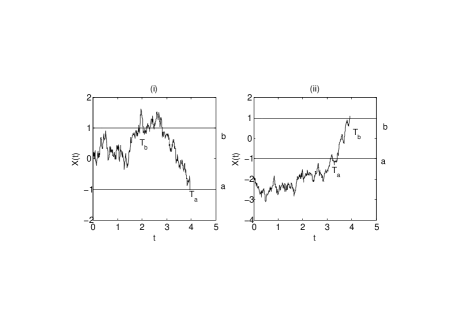
The quantities (4) and (5) are useful for the computation of the joint density function of Tasubscriptπ‘‡π‘ŽT_{a} and Tbsubscript𝑇𝑏T_{b}. Two different instances arise according to the location of the starting point X​(t0)=x0𝑋subscript𝑑0subscriptπ‘₯0X(t_{0})=x_{0} with respect to the boundaries (cf. Figure 1).
Refer to caption
Figure 1: Sample path of a stochastic process through two constant boundaries aπ‘Ža and b𝑏b: i) x0∈(a,b)subscriptπ‘₯0π‘Žπ‘x_{0}\in(a,b); ii) x0βˆ‰(a,b)subscriptπ‘₯0π‘Žπ‘x_{0}\notin(a,b).

It holds:

Theorem 2.1

Let X={X​(t),tβ‰₯t0}𝑋𝑋𝑑𝑑subscript𝑑0X=\{X(t),t\geq t_{0}\} be a diffusion process such that X​(t0)=x0𝑋subscript𝑑0subscriptπ‘₯0X(t_{0})=x_{0} and let a​(t)π‘Žπ‘‘a(t) and b​(t)𝑏𝑑b(t) be two continuous time dependent boundaries.

  1. i)

    If x0<a​(t0)<b​(t0)subscriptπ‘₯0π‘Žsubscript𝑑0𝑏subscript𝑑0x_{0}<a(t_{0})<b(t_{0}) and a​(t)<b​(t)π‘Žπ‘‘π‘π‘‘a(t)<b(t) for each t>t0𝑑subscript𝑑0t>t_{0} or b​(t0)<a​(t0)<x0𝑏subscript𝑑0π‘Žsubscript𝑑0subscriptπ‘₯0b(t_{0})<a(t_{0})<x_{0} and b​(t)<a​(t)π‘π‘‘π‘Žπ‘‘b(t)<a(t) for each t>t0𝑑subscript𝑑0t>t_{0}, then

    fTa,Tb​(t,s|x0,t0)={0tβ‰₯sfTa​(t|x0,t0)​fTb​(s|a​(t),t)t<s.subscript𝑓subscriptπ‘‡π‘Žsubscript𝑇𝑏𝑑conditional𝑠subscriptπ‘₯0subscript𝑑0cases0𝑑𝑠subscript𝑓subscriptπ‘‡π‘Žconditional𝑑subscriptπ‘₯0subscript𝑑0subscript𝑓subscript𝑇𝑏conditionalπ‘ π‘Žπ‘‘π‘‘π‘‘π‘ f_{T_{a},T_{b}}\left(t,s|x_{0},t_{0}\right)=\left\{\begin{array}[]{ll}0&t\geq s\\ f_{T_{a}}(t|x_{0},t_{0})f_{T_{b}}(s|a(t),t)&t<s\\ \end{array}.\right. (9)
  2. ii)

    If a​(t0)<x0<b​(t0)π‘Žsubscript𝑑0subscriptπ‘₯0𝑏subscript𝑑0a(t_{0})<x_{0}<b(t_{0}) and a​(t)<b​(t)π‘Žπ‘‘π‘π‘‘a(t)<b(t) for each t>t0𝑑subscript𝑑0t>t_{0}, then

    fTa​Tb​(t,s|x0,t0)={fTb​(s|a​(t),t)​ga​(t|x0,t0)t<s0t=sfTa​(t|b​(s),s)​gb​(s|x0,t0)t>s.subscript𝑓subscriptπ‘‡π‘Žsubscript𝑇𝑏𝑑conditional𝑠subscriptπ‘₯0subscript𝑑0casessubscript𝑓subscript𝑇𝑏conditionalπ‘ π‘Žπ‘‘π‘‘subscriptπ‘”π‘Žconditional𝑑subscriptπ‘₯0subscript𝑑0𝑑𝑠0𝑑𝑠subscript𝑓subscriptπ‘‡π‘Žconditional𝑑𝑏𝑠𝑠subscript𝑔𝑏conditional𝑠subscriptπ‘₯0subscript𝑑0𝑑𝑠f_{T_{a}T_{b}}\left(t,s|x_{0},t_{0}\right)=\left\{\begin{array}[]{ll}f_{T_{b}}(s|a(t),t)g_{a}(t|x_{0},t_{0})&t<s\\ 0&t=s\\ f_{T_{a}}(t|b(s),s)g_{b}(s|x_{0},t_{0})&t>s\\ \end{array}.\right. (10)

We omit the proof that is straightforward using the strong Markov property.

Remark 2.2

Note that the FPT pdf verifies the initial condition

limsβ†’tfTb​(s|a​(t),t)=limtβ†’sfTa​(t|b​(s),s)=0.subscript→𝑠𝑑subscript𝑓subscript𝑇𝑏conditionalπ‘ π‘Žπ‘‘π‘‘subscript→𝑑𝑠subscript𝑓subscriptπ‘‡π‘Žconditional𝑑𝑏𝑠𝑠0\displaystyle\lim_{s\rightarrow t}f_{T_{b}}(s|a(t),t)=\lim_{t\rightarrow s}f_{T_{a}}(t|b(s),s)=0. (11)

Furthermore, due to the differentiability of the boundaries, it holds (cf. [34])

limtβ†’sFX​(t)​(b​(t)|b​(s),s)subscript→𝑑𝑠subscript𝐹𝑋𝑑conditional𝑏𝑑𝑏𝑠𝑠\displaystyle\lim_{t\rightarrow s}F_{X(t)}(b(t)|b(s),s) =\displaystyle= limtβ†’sFX​(t)​(a​(t)|a​(s),s)=12subscript→𝑑𝑠subscript𝐹𝑋𝑑conditionalπ‘Žπ‘‘π‘Žπ‘ π‘ 12\displaystyle\lim_{t\rightarrow s}F_{X(t)}(a(t)|a(s),s)=\frac{1}{2} (12)
limtβ†’s[1βˆ’FX​(t)​(b​(t)|a​(s),s)]subscript→𝑑𝑠delimited-[]1subscript𝐹𝑋𝑑conditionalπ‘π‘‘π‘Žπ‘ π‘ \displaystyle\lim_{t\rightarrow s}[1-F_{X(t)}(b(t)|a(s),s)] =\displaystyle= limtβ†’sFX​(t)​(a​(t)|b​(s),s)=0.subscript→𝑑𝑠subscript𝐹𝑋𝑑conditionalπ‘Žπ‘‘π‘π‘ π‘ 0\displaystyle\lim_{t\rightarrow s}F_{X(t)}(a(t)|b(s),s)=0. (13)
Remark 2.3

For some applications it might be interesting to determine the copula function (cf.[24]) between Tasubscriptπ‘‡π‘ŽT_{a} and Tbsubscript𝑇𝑏T_{b}. When the two densities ga​(t|x0,t0)subscriptπ‘”π‘Žconditional𝑑subscriptπ‘₯0subscript𝑑0g_{a}(t|x_{0},t_{0}) and gb​(t|x0,t0)subscript𝑔𝑏conditional𝑑subscriptπ‘₯0subscript𝑑0g_{b}(t|x_{0},t_{0}) are known, use of (9) and (10) allows to determine this function.

3 System of integral equations

The computation of fTa​Tb​(t,s|x0,t0)subscript𝑓subscriptπ‘‡π‘Žsubscript𝑇𝑏𝑑conditional𝑠subscriptπ‘₯0subscript𝑑0f_{T_{a}T_{b}}\left(t,s|x_{0},t_{0}\right) involves the transition pdfs fTb​(s|a​(t),t)subscript𝑓subscript𝑇𝑏conditionalπ‘ π‘Žπ‘‘π‘‘f_{T_{b}}(s|a(t),t) and fTa​(t|b​(s),s)subscript𝑓subscriptπ‘‡π‘Žconditional𝑑𝑏𝑠𝑠f_{T_{a}}(t|b(s),s) and the terms ga​(t|x0,t0)subscriptπ‘”π‘Žconditional𝑑subscriptπ‘₯0subscript𝑑0g_{a}(t|x_{0},t_{0}) and gb​(t|x0,t0)subscript𝑔𝑏conditional𝑑subscriptπ‘₯0subscript𝑑0g_{b}(t|x_{0},t_{0}). When the process is a linear regular diffusion, the transition pdf is available in closed form and, if the process is strictly linear, it is Gaussian. In the literature, transition pdf is also available for other regular diffusion processes, such as the Cox-Ingersoll-Ross model (also known as Feller process), the Bessel process or some instances of the Raleigh process (cf. [17, 16]). Further examples arise from space-time transformation of the Brownian motion (cf. [30]) or of the Cox-Ingersol-Ross process (cf. [11]). When closed form solutions are not available, the transition pdf is evaluated resorting to numerical methods, such as the numerical solution of the Kolmogorov equation [21, 36] or the numerical inversion of Fourier transforms [40]. Unfortunately closed form expressions for the densities ga​(t|x0,t0)subscriptπ‘”π‘Žconditional𝑑subscriptπ‘₯0subscript𝑑0g_{a}(t|x_{0},t_{0}) and gb​(t|x0,t0)subscript𝑔𝑏conditional𝑑subscriptπ‘₯0subscript𝑑0g_{b}(t|x_{0},t_{0}) are known only for the Brownian motion with constant boundaries (cf. [8] formula 3.0.6) or for processes related to it through suitable transformations. Use of the following theorem helps to overcome this problem.

Theorem 3.1

Let X={X​(t),tβ‰₯t0}𝑋𝑋𝑑𝑑subscript𝑑0X=\{X(t),t\geq t_{0}\} be a diffusion process such that X​(t0)=x0𝑋subscript𝑑0subscriptπ‘₯0X(t_{0})=x_{0}. Let a​(t)π‘Žπ‘‘a(t) and b​(t)𝑏𝑑b(t) be two time dependent boundaries with bounded derivatives such that a​(t0)<x0<b​(t0)π‘Žsubscript𝑑0subscriptπ‘₯0𝑏subscript𝑑0a(t_{0})<x_{0}<b(t_{0}) and a​(t)<b​(t)π‘Žπ‘‘π‘π‘‘a(t)<b(t) for each t>t0𝑑subscript𝑑0t>t_{0}. The pdf’s ga​(t|x0,t0)subscriptπ‘”π‘Žconditional𝑑subscriptπ‘₯0subscript𝑑0g_{a}(t|x_{0},t_{0}) and gb​(t|x0,t0)subscript𝑔𝑏conditional𝑑subscriptπ‘₯0subscript𝑑0g_{b}(t|x_{0},t_{0}) are solution of the following system of Volterra first kind integral equations

1βˆ’FX​(t)​(b​(t)|x0,t0)1subscript𝐹𝑋𝑑conditional𝑏𝑑subscriptπ‘₯0subscript𝑑0\displaystyle 1-F_{X(t)}(b(t)|x_{0},t_{0}) =∫t0t[1βˆ’FX​(t)​(b​(t)|a​(Ο„),Ο„)]​ga​(Ο„|x0,t0)​𝑑τabsentsuperscriptsubscriptsubscript𝑑0𝑑delimited-[]1subscript𝐹𝑋𝑑conditionalπ‘π‘‘π‘Žπœπœsubscriptπ‘”π‘Žconditional𝜏subscriptπ‘₯0subscript𝑑0differential-d𝜏\displaystyle=\int_{t_{0}}^{t}\left[1-F_{X(t)}(b(t)|a(\tau),\tau)\right]g_{a}(\tau|x_{0},t_{0})d\tau (14a)
+∫t0t[1βˆ’FX​(t)​(b​(t)|b​(Ο„),Ο„)]​gb​(Ο„|x0,t0)​𝑑τsuperscriptsubscriptsubscript𝑑0𝑑delimited-[]1subscript𝐹𝑋𝑑conditionalπ‘π‘‘π‘πœπœsubscript𝑔𝑏conditional𝜏subscriptπ‘₯0subscript𝑑0differential-d𝜏\displaystyle+\int_{t_{0}}^{t}\left[1-F_{X(t)}(b(t)|b(\tau),\tau)\right]g_{b}(\tau|x_{0},t_{0})d\tau
FX​(t)​(a​(t)|x0,t0)subscript𝐹𝑋𝑑conditionalπ‘Žπ‘‘subscriptπ‘₯0subscript𝑑0\displaystyle F_{X(t)}(a(t)|x_{0},t_{0}) =∫t0tFX​(t)​(a​(t)|a​(Ο„),Ο„)​ga​(Ο„|x0,t0)​𝑑τabsentsuperscriptsubscriptsubscript𝑑0𝑑subscript𝐹𝑋𝑑conditionalπ‘Žπ‘‘π‘Žπœπœsubscriptπ‘”π‘Žconditional𝜏subscriptπ‘₯0subscript𝑑0differential-d𝜏\displaystyle=\int_{t_{0}}^{t}F_{X(t)}(a(t)|a(\tau),\tau)g_{a}(\tau|x_{0},t_{0})d\tau (14b)
+∫t0tFX​(t)​(a​(t)|b​(Ο„),Ο„)​gb​(Ο„|x0,t0)​𝑑τ.superscriptsubscriptsubscript𝑑0𝑑subscript𝐹𝑋𝑑conditionalπ‘Žπ‘‘π‘πœπœsubscript𝑔𝑏conditional𝜏subscriptπ‘₯0subscript𝑑0differential-d𝜏\displaystyle+\int_{t_{0}}^{t}F_{X(t)}(a(t)|b(\tau),\tau)g_{b}(\tau|x_{0},t_{0})d\tau.
Proof 3.2

For t∈[0,∞]𝑑0t\in[0,\infty], conditioning on the boundary first attained by the process, for xβˆ‰[a​(t),b​(t)]π‘₯π‘Žπ‘‘π‘π‘‘x\notin[a(t),b(t)] we get

P​(X​(t)≀x|X​(t0)=x0)𝑃𝑋𝑑conditionalπ‘₯𝑋subscript𝑑0subscriptπ‘₯0\displaystyle P\left(X(t)\leq x|X(t_{0})=x_{0}\right) =\displaystyle= ∫t0tP(X(t)≀x|Ta<Tb,Ta=Ο„,X(t0)=x0)ga(Ο„|x0,t0)dΟ„\displaystyle\int^{t}_{t_{0}}P\left(X(t)\leq x|T_{a}<T_{b},T_{a}=\tau,X(t_{0})=x_{0}\right)g_{a}(\tau|x_{0},t_{0})d\tau
+\displaystyle+ ∫t0tP​(X​(t)≀x​|Ta>​Tb,Tb=Ο„,X​(t0)=x0)​gb​(Ο„|x0,t0)​𝑑τsubscriptsuperscript𝑑subscript𝑑0𝑃formulae-sequence𝑋𝑑π‘₯ketsubscriptπ‘‡π‘Žsubscript𝑇𝑏formulae-sequencesubscriptπ‘‡π‘πœπ‘‹subscript𝑑0subscriptπ‘₯0subscript𝑔𝑏conditional𝜏subscriptπ‘₯0subscript𝑑0differential-d𝜏\displaystyle\int^{t}_{t_{0}}P\left(X(t)\leq x|T_{a}>T_{b},T_{b}=\tau,X(t_{0})=x_{0}\right)g_{b}(\tau|x_{0},t_{0})d\tau
=\displaystyle= ∫t0tP(X(t)≀x|X(Ο„)=a(Ο„),X(t0)=x0)ga(Ο„|x0,t0)dΟ„\displaystyle\int^{t}_{t_{0}}P\left(X(t)\leq x|X(\tau)=a(\tau),X(t_{0})=x_{0}\right)g_{a}(\tau|x_{0},t_{0})d\tau
+\displaystyle+ ∫t0tP(X(t)≀x|X(Ο„)=b(Ο„),X(t0)=x0)gb(Ο„|x0,t0)dΟ„.\displaystyle\int^{t}_{t_{0}}P\left(X(t)\leq x|X(\tau)=b(\tau),X(t_{0})=x_{0}\right)g_{b}(\tau|x_{0},t_{0})d\tau.

Differentiating with respect to xπ‘₯x we obtain

fX​(t)​(x|x0,t0)subscript𝑓𝑋𝑑conditionalπ‘₯subscriptπ‘₯0subscript𝑑0\displaystyle f_{X(t)}(x|x_{0},t_{0}) =\displaystyle= ∫t0tfX​(t)​(x|a​(Ο„),Ο„)​ga​(Ο„|x0,t0)​𝑑τsuperscriptsubscriptsubscript𝑑0𝑑subscript𝑓𝑋𝑑conditionalπ‘₯π‘Žπœπœsubscriptπ‘”π‘Žconditional𝜏subscriptπ‘₯0subscript𝑑0differential-d𝜏\displaystyle\int_{t_{0}}^{t}f_{X(t)}(x|a(\tau),\tau)g_{a}(\tau|x_{0},t_{0})d\tau
+\displaystyle+ ∫t0tfX​(t)​(x|b​(Ο„),Ο„)​gb​(Ο„|x0,t0)​𝑑τ.superscriptsubscriptsubscript𝑑0𝑑subscript𝑓𝑋𝑑conditionalπ‘₯π‘πœπœsubscript𝑔𝑏conditional𝜏subscriptπ‘₯0subscript𝑑0differential-d𝜏\displaystyle\int_{t_{0}}^{t}f_{X(t)}(x|b(\tau),\tau)g_{b}(\tau|x_{0},t_{0})d\tau.

Integrating (3.2) with respect to xπ‘₯x on the two subdomains [b​(t),∞]𝑏𝑑[b(t),\infty] and [βˆ’βˆž,a​(t)]π‘Žπ‘‘[-\infty,a(t)] respectively, we get (14a) and (14b).

Remark 3.3

Differentiating (14a) and (14b) with respect to t𝑑t and recalling (12) and (13) one gets

gb​(t|x0,t0)subscript𝑔𝑏conditional𝑑subscriptπ‘₯0subscript𝑑0\displaystyle g_{b}(t|x_{0},t_{0}) =βˆ’2β€‹βˆ‚FX​(t)​(b​(t)|x0,t0)βˆ‚tabsent2subscript𝐹𝑋𝑑conditional𝑏𝑑subscriptπ‘₯0subscript𝑑0𝑑\displaystyle=-2\frac{\partial F_{X(t)}(b(t)|x_{0},t_{0})}{\partial t} (16a)
+∫t0t2​(βˆ‚FX​(t)​(b​(t)|a​(Ο„),Ο„)βˆ‚t​ga​(Ο„|x0,t0)+βˆ‚FX​(t)​(b​(t)|b​(Ο„),Ο„)βˆ‚t​gb​(Ο„|x0,t0))​𝑑τ.superscriptsubscriptsubscript𝑑0𝑑2subscript𝐹𝑋𝑑conditionalπ‘π‘‘π‘Žπœπœπ‘‘subscriptπ‘”π‘Žconditional𝜏subscriptπ‘₯0subscript𝑑0subscript𝐹𝑋𝑑conditionalπ‘π‘‘π‘πœπœπ‘‘subscript𝑔𝑏conditional𝜏subscriptπ‘₯0subscript𝑑0differential-d𝜏\displaystyle+\int_{t_{0}}^{t}2\left(\frac{\partial F_{X(t)}(b(t)|a(\tau),\tau)}{\partial t}g_{a}(\tau|x_{0},t_{0})+\frac{\partial F_{X(t)}(b(t)|b(\tau),\tau)}{\partial t}g_{b}(\tau|x_{0},t_{0})\right)d\tau.
ga​(t|x0,t0)subscriptπ‘”π‘Žconditional𝑑subscriptπ‘₯0subscript𝑑0\displaystyle g_{a}(t|x_{0},t_{0}) =2β€‹βˆ‚FX​(t)​(a​(t)|x0,t0)βˆ‚tabsent2subscript𝐹𝑋𝑑conditionalπ‘Žπ‘‘subscriptπ‘₯0subscript𝑑0𝑑\displaystyle=2\frac{\partial F_{X(t)}(a(t)|x_{0},t_{0})}{\partial t} (16b)
βˆ’βˆ«t0t2​(βˆ‚FX​(t)​(a​(t)|a​(Ο„),Ο„)βˆ‚t​ga​(Ο„|x0,t0)+βˆ‚FX​(t)​(a​(t)|b​(Ο„),Ο„)βˆ‚t​gb​(Ο„|x0,t0))​𝑑τ.superscriptsubscriptsubscript𝑑0𝑑2subscript𝐹𝑋𝑑conditionalπ‘Žπ‘‘π‘Žπœπœπ‘‘subscriptπ‘”π‘Žconditional𝜏subscriptπ‘₯0subscript𝑑0subscript𝐹𝑋𝑑conditionalπ‘Žπ‘‘π‘πœπœπ‘‘subscript𝑔𝑏conditional𝜏subscriptπ‘₯0subscript𝑑0differential-d𝜏\displaystyle-\int_{t_{0}}^{t}2\left(\frac{\partial F_{X(t)}(a(t)|a(\tau),\tau)}{\partial t}g_{a}(\tau|x_{0},t_{0})+\frac{\partial F_{X(t)}(a(t)|b(\tau),\tau)}{\partial t}g_{b}(\tau|x_{0},t_{0})\right)d\tau.

This system of Volterra integral equations coincides with the one proposed in [9] if the kernel of the two equations is regularized.

It holds

Theorem 3.4

The system (14) has a unique continuous solution for t>t0𝑑subscript𝑑0t>t_{0}.

Proof 3.5

The system of Volterra integral equations of the first kind (14) is equivalent to the system of Volterra integral equations of the second kind (16) that can be written in matricial form

g​(t)=h​(t)+∫t0tk​(t,Ο„)​g​(Ο„)​𝑑τg𝑑h𝑑superscriptsubscriptsubscript𝑑0𝑑kπ‘‘πœg𝜏differential-d𝜏\text{{g}}(t)=\text{{h}}(t)+\int_{t_{0}}^{t}\text{{k}}(t,\tau)\text{{g}}(\tau)d\tau (17)

where

g​(t)=[ga​(t|x0,t0)gb​(t|x0,t0)],g𝑑delimited-[]subscriptπ‘”π‘Žconditional𝑑subscriptπ‘₯0subscript𝑑0subscript𝑔𝑏conditional𝑑subscriptπ‘₯0subscript𝑑0\text{{g}}(t)=\left[\begin{array}[]{c}g_{a}(t|x_{0},t_{0})\\ g_{b}(t|x_{0},t_{0})\end{array}\right], (18)
h​(t)=[βˆ’2β€‹βˆ‚FX​(t)​(b​(t)|x0,t0)βˆ‚t2β€‹βˆ‚FX​(t)​(a​(t)|x0,t0)βˆ‚t],h𝑑delimited-[]2subscript𝐹𝑋𝑑conditional𝑏𝑑subscriptπ‘₯0subscript𝑑0𝑑2subscript𝐹𝑋𝑑conditionalπ‘Žπ‘‘subscriptπ‘₯0subscript𝑑0𝑑\text{{h}}(t)=\left[\begin{array}[]{c}-2\frac{\partial F_{X(t)}(b(t)|x_{0},t_{0})}{\partial t}\\ 2\frac{\partial F_{X(t)}(a(t)|x_{0},t_{0})}{\partial t}\end{array}\right], (19)
k​(t,Ο„)=[βˆ’2β€‹βˆ‚FX​(t)​(b​(t)|a​(Ο„),Ο„)βˆ‚tβˆ’2β€‹βˆ‚FX​(t)​(b​(t)|b​(Ο„),Ο„)βˆ‚t2β€‹βˆ‚FX​(t)​(a​(t)|a​(Ο„),Ο„)βˆ‚t2β€‹βˆ‚FX​(t)​(a​(t)|b​(Ο„),Ο„)βˆ‚t],kπ‘‘πœdelimited-[]2subscript𝐹𝑋𝑑conditionalπ‘π‘‘π‘Žπœπœπ‘‘2subscript𝐹𝑋𝑑conditionalπ‘π‘‘π‘πœπœπ‘‘2subscript𝐹𝑋𝑑conditionalπ‘Žπ‘‘π‘Žπœπœπ‘‘2subscript𝐹𝑋𝑑conditionalπ‘Žπ‘‘π‘πœπœπ‘‘\text{{k}}(t,\tau)=\left[\begin{array}[]{cc}-2\frac{\partial F_{X(t)}(b(t)|a(\tau),\tau)}{\partial t}&-2\frac{\partial F_{X(t)}(b(t)|b(\tau),\tau)}{\partial t}\\ 2\frac{\partial F_{X(t)}(a(t)|a(\tau),\tau)}{\partial t}&2\frac{\partial F_{X(t)}(a(t)|b(\tau),\tau)}{\partial t}\end{array}\right], (20)

Since the kernel k​(t,Ο„)kπ‘‘πœ\text{{k}}(t,\tau) is singular in Ο„=tπœπ‘‘\tau=t, we introduce an equivalent system with continuous kernel. Mimicking the method presented in [10], we introduce two couple of functions Ξ³i​(t)subscript𝛾𝑖𝑑\gamma_{i}(t) and Ξ·i​(t)subscriptπœ‚π‘–π‘‘\eta_{i}(t), i=1,2𝑖12i=1,2, continuous in [t0,+∞]subscript𝑑0[t_{0},+\infty]. Combining (14), (3.2) and (16), together with Ξ³i​(t)subscript𝛾𝑖𝑑\gamma_{i}(t) and Ξ·i​(t)subscriptπœ‚π‘–π‘‘\eta_{i}(t) we obtain

gb​(t|x0,t0)=βˆ’Ξ¨1​(b​(t)|x0,t0)+∫t0t(Ξ¨1​(b​(t)|a​(Ο„),Ο„)​ga​(Ο„|x0,t0)+Ξ¨1​(b​(t)|b​(Ο„),Ο„)​gb​(Ο„|x0,t0))​𝑑τ.subscript𝑔𝑏conditional𝑑subscriptπ‘₯0subscript𝑑0superscriptΞ¨1conditional𝑏𝑑subscriptπ‘₯0subscript𝑑0superscriptsubscriptsubscript𝑑0𝑑superscriptΞ¨1conditionalπ‘π‘‘π‘Žπœπœsubscriptπ‘”π‘Žconditional𝜏subscriptπ‘₯0subscript𝑑0superscriptΞ¨1conditionalπ‘π‘‘π‘πœπœsubscript𝑔𝑏conditional𝜏subscriptπ‘₯0subscript𝑑0differential-d𝜏\displaystyle g_{b}(t|x_{0},t_{0})=-\Psi^{1}(b(t)|x_{0},t_{0})+\int_{t_{0}}^{t}\left(\Psi^{1}(b(t)|a(\tau),\tau)g_{a}(\tau|x_{0},t_{0})+\Psi^{1}(b(t)|b(\tau),\tau)g_{b}(\tau|x_{0},t_{0})\right)d\tau.
ga​(t|x0,t0)=Ξ¨2​(a​(t)|x0,t0)βˆ’βˆ«t0t(Ξ¨2​(a​(t)|a​(Ο„),Ο„)​ga​(Ο„|x0,t0)+Ξ¨2​(a​(t)|b​(Ο„),Ο„)​gb​(Ο„|x0,t0))​𝑑τ.subscriptπ‘”π‘Žconditional𝑑subscriptπ‘₯0subscript𝑑0superscriptΞ¨2conditionalπ‘Žπ‘‘subscriptπ‘₯0subscript𝑑0superscriptsubscriptsubscript𝑑0𝑑superscriptΞ¨2conditionalπ‘Žπ‘‘π‘Žπœπœsubscriptπ‘”π‘Žconditional𝜏subscriptπ‘₯0subscript𝑑0superscriptΞ¨2conditionalπ‘Žπ‘‘π‘πœπœsubscript𝑔𝑏conditional𝜏subscriptπ‘₯0subscript𝑑0differential-d𝜏\displaystyle g_{a}(t|x_{0},t_{0})=\Psi^{2}(a(t)|x_{0},t_{0})-\int_{t_{0}}^{t}\left(\Psi^{2}(a(t)|a(\tau),\tau)g_{a}(\tau|x_{0},t_{0})+\Psi^{2}(a(t)|b(\tau),\tau)g_{b}(\tau|x_{0},t_{0})\right)d\tau. (21)

where

Ξ¨1​(b​(t)|x,s)superscriptΞ¨1conditional𝑏𝑑π‘₯𝑠\displaystyle\Psi^{1}(b(t)|x,s) =\displaystyle= βˆ’2β€‹βˆ‚FX​(t)​(b​(t)|x,s)βˆ‚t+Ξ³1​(t)​fX​(t)​(b​(t),t|x,s)+Ξ·1​(t)​[1βˆ’FX​(t)​(b​(t)|x,s)]2subscript𝐹𝑋𝑑conditional𝑏𝑑π‘₯𝑠𝑑subscript𝛾1𝑑subscript𝑓𝑋𝑑𝑏𝑑conditional𝑑π‘₯𝑠subscriptπœ‚1𝑑delimited-[]1subscript𝐹𝑋𝑑conditional𝑏𝑑π‘₯𝑠\displaystyle-2\frac{\partial F_{X(t)}(b(t)|x,s)}{\partial t}+\gamma_{1}(t)f_{X(t)}(b(t),t|x,s)+\eta_{1}(t)[1-F_{X(t)}(b(t)|x,s)]
Ξ¨2​(a​(t)|x,s)superscriptΞ¨2conditionalπ‘Žπ‘‘π‘₯𝑠\displaystyle\Psi^{2}(a(t)|x,s) =\displaystyle= 2β€‹βˆ‚FX​(t)​(a​(t)|x,s)βˆ‚tβˆ’Ξ³2​(t)​fX​(t)​(a​(t),t|x,s)βˆ’Ξ·2​(t)​FX​(t)​(a​(t)|x,s)2subscript𝐹𝑋𝑑conditionalπ‘Žπ‘‘π‘₯𝑠𝑑subscript𝛾2𝑑subscriptπ‘“π‘‹π‘‘π‘Žπ‘‘conditional𝑑π‘₯𝑠subscriptπœ‚2𝑑subscript𝐹𝑋𝑑conditionalπ‘Žπ‘‘π‘₯𝑠\displaystyle 2\frac{\partial F_{X(t)}(a(t)|x,s)}{\partial t}-\gamma_{2}(t)f_{X(t)}(a(t),t|x,s)-\eta_{2}(t)F_{X(t)}(a(t)|x,s) (22)

A suitable choice of Ξ³i​(t)subscript𝛾𝑖𝑑\gamma_{i}(t) and Ξ·i​(t)subscriptπœ‚π‘–π‘‘\eta_{i}(t), i=1,2𝑖12i=1,2, makes Ξ¨1​(b​(t)|b​(Ο„),Ο„)superscriptΞ¨1conditionalπ‘π‘‘π‘πœπœ\Psi^{1}(b(t)|b(\tau),\tau) and Ξ¨2​(a​(t)|a​(Ο„),Ο„)superscriptΞ¨2conditionalπ‘Žπ‘‘π‘Žπœπœ\Psi^{2}(a(t)|a(\tau),\tau) not singular. On the other hand, since (cf. [9])

limΟ„β†’tfX​(t)​(b​(t),t|a​(Ο„),Ο„)subscriptβ†’πœπ‘‘subscript𝑓𝑋𝑑𝑏𝑑conditionalπ‘‘π‘Žπœπœ\displaystyle\lim_{\tau\rightarrow t}f_{X(t)}(b(t),t|a(\tau),\tau) =limΟ„β†’tβˆ‚βˆ‚x​fX​(t)​(x,t|a​(Ο„),Ο„)|x=b​(t)=0absentevaluated-atsubscriptβ†’πœπ‘‘π‘₯subscript𝑓𝑋𝑑π‘₯conditionalπ‘‘π‘Žπœπœπ‘₯𝑏𝑑0\displaystyle=\left.\lim_{\tau\rightarrow t}\frac{\partial}{\partial x}f_{X(t)}(x,t|a(\tau),\tau)\right|_{x=b(t)}=0 (23)
limΟ„β†’tfX​(t)​(a​(t),t|b​(Ο„),Ο„)subscriptβ†’πœπ‘‘subscriptπ‘“π‘‹π‘‘π‘Žπ‘‘conditionalπ‘‘π‘πœπœ\displaystyle\lim_{\tau\rightarrow t}f_{X(t)}(a(t),t|b(\tau),\tau) =limΟ„β†’tβˆ‚βˆ‚x​fX​(t)​(x,t|b​(Ο„),Ο„)|x=a​(t)=0,absentevaluated-atsubscriptβ†’πœπ‘‘π‘₯subscript𝑓𝑋𝑑π‘₯conditionalπ‘‘π‘πœπœπ‘₯π‘Žπ‘‘0\displaystyle=\left.\lim_{\tau\rightarrow t}\frac{\partial}{\partial x}f_{X(t)}(x,t|b(\tau),\tau)\right|_{x=a(t)}=0,

the kernels Ξ¨1​(b​(t)|a​(Ο„),Ο„)superscriptΞ¨1conditionalπ‘π‘‘π‘Žπœπœ\Psi^{1}(b(t)|a(\tau),\tau) and Ξ¨2​(a​(t)|b​(Ο„),Ο„)superscriptΞ¨2conditionalπ‘Žπ‘‘π‘πœπœ\Psi^{2}(a(t)|b(\tau),\tau) are not singular. This makes possible to apply Theorem 3.11 of [23] to get the thesis.

Remark 3.6

The functions Ξ³i​(t)subscript𝛾𝑖𝑑\gamma_{i}(t) and Ξ·i​(t)subscriptπœ‚π‘–π‘‘\eta_{i}(t), i=1,2𝑖12i=1,2 can be determined. For example, for an Ornstein Uhlenbeck process characterized by the drift μ​(t,x)=α​x+Ξ²πœ‡π‘‘π‘₯𝛼π‘₯𝛽\mu(t,x)=\alpha x+\beta and infinitesimal variance σ​(t,x)=ΟƒπœŽπ‘‘π‘₯𝜎\sigma(t,x)=\sigma, where α𝛼\alpha, β𝛽\beta and Οƒ>0𝜎0\sigma>0 are arbitrary real constants. The functions that regularize the kernels are Ξ³1​(t)=1/2​[α​b​(t)+Ξ²βˆ’b′​(t)]subscript𝛾1𝑑12delimited-[]𝛼𝑏𝑑𝛽superscript𝑏′𝑑\gamma_{1}(t)=1/2[\alpha b(t)+\beta-b^{\prime}(t)], Ξ³2​(t)=1/2​[α​a​(t)+Ξ²βˆ’a′​(t)]subscript𝛾2𝑑12delimited-[]π›Όπ‘Žπ‘‘π›½superscriptπ‘Žβ€²π‘‘\gamma_{2}(t)=1/2[\alpha a(t)+\beta-a^{\prime}(t)] and Ξ·i​(t)≑0subscriptπœ‚π‘–π‘‘0\eta_{i}(t)\equiv 0, i=1,2𝑖12i=1,2 (cf. [10]).

When the boundaries are constant it holds:

Corollary 3.7

Let X={X​(t),tβ‰₯t0}𝑋𝑋𝑑𝑑subscript𝑑0X=\{X(t),t\geq t_{0}\} be a diffusion process such that X​(t0)=x0𝑋subscript𝑑0subscriptπ‘₯0X(t_{0})=x_{0} and let aπ‘Ža and b𝑏b be two constant boundaries such that a<x0<bπ‘Žsubscriptπ‘₯0𝑏a<x_{0}<b, then the following three expressions are equivalent for gaλ​(x0)=∫t0+∞eβˆ’Ξ»β€‹t​ga​(t|x0,t0)​𝑑tsuperscriptsubscriptπ‘”π‘Žπœ†subscriptπ‘₯0superscriptsubscriptsubscript𝑑0superscriptπ‘’πœ†π‘‘subscriptπ‘”π‘Žconditional𝑑subscriptπ‘₯0subscript𝑑0differential-d𝑑g_{a}^{\lambda}(x_{0})=\int_{t_{0}}^{+\infty}e^{-\lambda t}g_{a}(t|x_{0},t_{0})dt and gbλ​(x0)=∫t0+∞eβˆ’Ξ»β€‹t​gb​(t|x0,t0)​𝑑tsuperscriptsubscriptπ‘”π‘πœ†subscriptπ‘₯0superscriptsubscriptsubscript𝑑0superscriptπ‘’πœ†π‘‘subscript𝑔𝑏conditional𝑑subscriptπ‘₯0subscript𝑑0differential-d𝑑g_{b}^{\lambda}(x_{0})=\int_{t_{0}}^{+\infty}e^{-\lambda t}g_{b}(t|x_{0},t_{0})dt:

gaλ​(x0)superscriptsubscriptπ‘”π‘Žπœ†subscriptπ‘₯0\displaystyle g_{a}^{\lambda}(x_{0}) =fTbλ​(x0)​fTaλ​(b)βˆ’fTaλ​(x0)fTaλ​(b)​fTbλ​(a)βˆ’1absentsuperscriptsubscript𝑓subscriptπ‘‡π‘πœ†subscriptπ‘₯0superscriptsubscript𝑓subscriptπ‘‡π‘Žπœ†π‘superscriptsubscript𝑓subscriptπ‘‡π‘Žπœ†subscriptπ‘₯0superscriptsubscript𝑓subscriptπ‘‡π‘Žπœ†π‘superscriptsubscript𝑓subscriptπ‘‡π‘πœ†π‘Ž1\displaystyle=\frac{f_{T_{b}}^{\lambda}(x_{0})f_{T_{a}}^{\lambda}(b)-f_{T_{a}}^{\lambda}(x_{0})}{f_{T_{a}}^{\lambda}(b)f_{T_{b}}^{\lambda}(a)-1} (24a)
gbλ​(x0)superscriptsubscriptπ‘”π‘πœ†subscriptπ‘₯0\displaystyle g_{b}^{\lambda}(x_{0}) =fTaλ​(x0)​fTbλ​(a)βˆ’fTbλ​(x0)fTaλ​(b)​fTbλ​(a)βˆ’1absentsuperscriptsubscript𝑓subscriptπ‘‡π‘Žπœ†subscriptπ‘₯0superscriptsubscript𝑓subscriptπ‘‡π‘πœ†π‘Žsuperscriptsubscript𝑓subscriptπ‘‡π‘πœ†subscriptπ‘₯0superscriptsubscript𝑓subscriptπ‘‡π‘Žπœ†π‘superscriptsubscript𝑓subscriptπ‘‡π‘πœ†π‘Ž1\displaystyle=\frac{f_{T_{a}}^{\lambda}(x_{0})f_{T_{b}}^{\lambda}(a)-f_{T_{b}}^{\lambda}(x_{0})}{f_{T_{a}}^{\lambda}(b)f_{T_{b}}^{\lambda}(a)-1} (24b)
gaλ​(x0)superscriptsubscriptπ‘”π‘Žπœ†subscriptπ‘₯0\displaystyle g_{a}^{\lambda}(x_{0}) =[1βˆ’Ξ»β€‹FXλ​(b|x0)]​FXλ​(a|b)βˆ’[1βˆ’Ξ»β€‹FXλ​(b|b)]​FXλ​(a|x0)[1βˆ’Ξ»β€‹FXλ​(b|a)]​FXλ​(a|b)βˆ’[1βˆ’Ξ»β€‹FXλ​(b|b)]​FXλ​(a|a)absentdelimited-[]1πœ†superscriptsubscriptπΉπ‘‹πœ†conditional𝑏subscriptπ‘₯0superscriptsubscriptπΉπ‘‹πœ†conditionalπ‘Žπ‘delimited-[]1πœ†superscriptsubscriptπΉπ‘‹πœ†conditional𝑏𝑏superscriptsubscriptπΉπ‘‹πœ†conditionalπ‘Žsubscriptπ‘₯0delimited-[]1πœ†superscriptsubscriptπΉπ‘‹πœ†conditionalπ‘π‘ŽsuperscriptsubscriptπΉπ‘‹πœ†conditionalπ‘Žπ‘delimited-[]1πœ†superscriptsubscriptπΉπ‘‹πœ†conditional𝑏𝑏superscriptsubscriptπΉπ‘‹πœ†conditionalπ‘Žπ‘Ž\displaystyle=\frac{\left[1-\lambda F_{X}^{\lambda}(b|x_{0})\right]F_{X}^{\lambda}(a|b)-\left[1-\lambda F_{X}^{\lambda}(b|b)\right]F_{X}^{\lambda}(a|x_{0})}{\left[1-\lambda F_{X}^{\lambda}(b|a)\right]F_{X}^{\lambda}(a|b)-\left[1-\lambda F_{X}^{\lambda}(b|b)\right]F_{X}^{\lambda}(a|a)} (25a)
gbλ​(x0)superscriptsubscriptπ‘”π‘πœ†subscriptπ‘₯0\displaystyle g_{b}^{\lambda}(x_{0}) =[1βˆ’Ξ»β€‹FXλ​(b|x0)]​FXλ​(a|a)βˆ’[1βˆ’Ξ»β€‹FXλ​(b|a)]​FXλ​(a|x0)[1βˆ’Ξ»β€‹FXλ​(b|b)]​FXλ​(a|a)βˆ’[1βˆ’Ξ»β€‹FXλ​(b|a)]​FXλ​(a|b)absentdelimited-[]1πœ†superscriptsubscriptπΉπ‘‹πœ†conditional𝑏subscriptπ‘₯0superscriptsubscriptπΉπ‘‹πœ†conditionalπ‘Žπ‘Ždelimited-[]1πœ†superscriptsubscriptπΉπ‘‹πœ†conditionalπ‘π‘ŽsuperscriptsubscriptπΉπ‘‹πœ†conditionalπ‘Žsubscriptπ‘₯0delimited-[]1πœ†superscriptsubscriptπΉπ‘‹πœ†conditional𝑏𝑏superscriptsubscriptπΉπ‘‹πœ†conditionalπ‘Žπ‘Ždelimited-[]1πœ†superscriptsubscriptπΉπ‘‹πœ†conditionalπ‘π‘ŽsuperscriptsubscriptπΉπ‘‹πœ†conditionalπ‘Žπ‘\displaystyle=\frac{\left[1-\lambda F_{X}^{\lambda}(b|x_{0})\right]F_{X}^{\lambda}(a|a)-\left[1-\lambda F_{X}^{\lambda}(b|a)\right]F_{X}^{\lambda}(a|x_{0})}{\left[1-\lambda F_{X}^{\lambda}(b|b)\right]F_{X}^{\lambda}(a|a)-\left[1-\lambda F_{X}^{\lambda}(b|a)\right]F_{X}^{\lambda}(a|b)} (25b)
gaλ​(x0)superscriptsubscriptπ‘”π‘Žπœ†subscriptπ‘₯0\displaystyle g_{a}^{\lambda}(x_{0}) =fXλ​(x1|x0)​fXλ​(x2|b)βˆ’fXλ​(x1|b)​fXλ​(x2|x0)fXλ​(x1|a)​fXλ​(x2|b)βˆ’fXλ​(x1|b)​fXλ​(x2|a)absentsuperscriptsubscriptπ‘“π‘‹πœ†conditionalsubscriptπ‘₯1subscriptπ‘₯0superscriptsubscriptπ‘“π‘‹πœ†conditionalsubscriptπ‘₯2𝑏superscriptsubscriptπ‘“π‘‹πœ†conditionalsubscriptπ‘₯1𝑏superscriptsubscriptπ‘“π‘‹πœ†conditionalsubscriptπ‘₯2subscriptπ‘₯0superscriptsubscriptπ‘“π‘‹πœ†conditionalsubscriptπ‘₯1π‘Žsuperscriptsubscriptπ‘“π‘‹πœ†conditionalsubscriptπ‘₯2𝑏superscriptsubscriptπ‘“π‘‹πœ†conditionalsubscriptπ‘₯1𝑏superscriptsubscriptπ‘“π‘‹πœ†conditionalsubscriptπ‘₯2π‘Ž\displaystyle=\frac{f_{X}^{\lambda}(x_{1}|x_{0})f_{X}^{\lambda}(x_{2}|b)-f_{X}^{\lambda}(x_{1}|b)f_{X}^{\lambda}(x_{2}|x_{0})}{f_{X}^{\lambda}(x_{1}|a)f_{X}^{\lambda}(x_{2}|b)-f_{X}^{\lambda}(x_{1}|b)f_{X}^{\lambda}(x_{2}|a)}
=v1​(Ξ±,x0)​v2​(Ξ±,b)βˆ’v2​(Ξ±,x0)​v1​(Ξ±,b)v1​(Ξ±,a)​v2​(Ξ±,b)βˆ’v2​(Ξ±,a)​v1​(Ξ±,b)absentsubscript𝑣1𝛼subscriptπ‘₯0subscript𝑣2𝛼𝑏subscript𝑣2𝛼subscriptπ‘₯0subscript𝑣1𝛼𝑏subscript𝑣1π›Όπ‘Žsubscript𝑣2𝛼𝑏subscript𝑣2π›Όπ‘Žsubscript𝑣1𝛼𝑏\displaystyle=\frac{v_{1}(\alpha,x_{0})v_{2}(\alpha,b)-v_{2}(\alpha,x_{0})v_{1}(\alpha,b)}{v_{1}(\alpha,a)v_{2}(\alpha,b)-v_{2}(\alpha,a)v_{1}(\alpha,b)} (26a)
gbλ​(x0)superscriptsubscriptπ‘”π‘πœ†subscriptπ‘₯0\displaystyle g_{b}^{\lambda}(x_{0}) =fXλ​(x1|a)​fXλ​(x2|x0)βˆ’fXλ​(x1|x0)​fXλ​(x2|a)fXλ​(x1|a)​fXλ​(x2|b)βˆ’fXλ​(x1|b)​fXλ​(x2|a)absentsuperscriptsubscriptπ‘“π‘‹πœ†conditionalsubscriptπ‘₯1π‘Žsuperscriptsubscriptπ‘“π‘‹πœ†conditionalsubscriptπ‘₯2subscriptπ‘₯0superscriptsubscriptπ‘“π‘‹πœ†conditionalsubscriptπ‘₯1subscriptπ‘₯0superscriptsubscriptπ‘“π‘‹πœ†conditionalsubscriptπ‘₯2π‘Žsuperscriptsubscriptπ‘“π‘‹πœ†conditionalsubscriptπ‘₯1π‘Žsuperscriptsubscriptπ‘“π‘‹πœ†conditionalsubscriptπ‘₯2𝑏superscriptsubscriptπ‘“π‘‹πœ†conditionalsubscriptπ‘₯1𝑏superscriptsubscriptπ‘“π‘‹πœ†conditionalsubscriptπ‘₯2π‘Ž\displaystyle=\frac{f_{X}^{\lambda}(x_{1}|a)f_{X}^{\lambda}(x_{2}|x_{0})-f_{X}^{\lambda}(x_{1}|x_{0})f_{X}^{\lambda}(x_{2}|a)}{f_{X}^{\lambda}(x_{1}|a)f_{X}^{\lambda}(x_{2}|b)-f_{X}^{\lambda}(x_{1}|b)f_{X}^{\lambda}(x_{2}|a)}
=v1​(Ξ±,a)​v2​(Ξ±,x0)βˆ’v2​(Ξ±,a)​v1​(Ξ±,x0)v1​(Ξ±,a)​v2​(Ξ±,b)βˆ’v2​(Ξ±,a)​v1​(Ξ±,b)absentsubscript𝑣1π›Όπ‘Žsubscript𝑣2𝛼subscriptπ‘₯0subscript𝑣2π›Όπ‘Žsubscript𝑣1𝛼subscriptπ‘₯0subscript𝑣1π›Όπ‘Žsubscript𝑣2𝛼𝑏subscript𝑣2π›Όπ‘Žsubscript𝑣1𝛼𝑏\displaystyle=\frac{v_{1}(\alpha,a)v_{2}(\alpha,x_{0})-v_{2}(\alpha,a)v_{1}(\alpha,x_{0})}{v_{1}(\alpha,a)v_{2}(\alpha,b)-v_{2}(\alpha,a)v_{1}(\alpha,b)} (26b)

where

FXλ​(x|x0)superscriptsubscriptπΉπ‘‹πœ†conditionalπ‘₯subscriptπ‘₯0\displaystyle F_{X}^{\lambda}(x|x_{0}) =\displaystyle= ∫0+∞eβˆ’Ξ»β€‹t​FX​(t)​(x|x0,t0)​𝑑tsuperscriptsubscript0superscriptπ‘’πœ†π‘‘subscript𝐹𝑋𝑑conditionalπ‘₯subscriptπ‘₯0subscript𝑑0differential-d𝑑\displaystyle\int_{0}^{+\infty}e^{-\lambda t}F_{X(t)}(x|x_{0},t_{0})dt
fXλ​(x|x0)superscriptsubscriptπ‘“π‘‹πœ†conditionalπ‘₯subscriptπ‘₯0\displaystyle f_{X}^{\lambda}(x|x_{0}) =\displaystyle= ∫0+∞eβˆ’Ξ»β€‹t​fX​(t)​(x|x0,t0)​𝑑tsuperscriptsubscript0superscriptπ‘’πœ†π‘‘subscript𝑓𝑋𝑑conditionalπ‘₯subscriptπ‘₯0subscript𝑑0differential-d𝑑\displaystyle\int_{0}^{+\infty}e^{-\lambda t}f_{X(t)}(x|x_{0},t_{0})dt
fTaλ​(x0)superscriptsubscript𝑓subscriptπ‘‡π‘Žπœ†subscriptπ‘₯0\displaystyle f_{T_{a}}^{\lambda}(x_{0}) =\displaystyle= ∫0+∞eβˆ’Ξ»β€‹t​FTa​(t|x0,t0)​𝑑tsuperscriptsubscript0superscriptπ‘’πœ†π‘‘subscript𝐹subscriptπ‘‡π‘Žconditional𝑑subscriptπ‘₯0subscript𝑑0differential-d𝑑\displaystyle\int_{0}^{+\infty}e^{-\lambda t}F_{T_{a}}(t|x_{0},t_{0})dt

and the functions vi​(Ξ±,x)subscript𝑣𝑖𝛼π‘₯v_{i}(\alpha,x), i=1,2𝑖12i=1,2 are fundamental solutions of (8.13b) in [35].

Proof 3.8

Generalizing the standard calculation of p. 30 in [20] for an arbitrary regular diffusion we obtain (24).

Applying Laplace transform to (14) and using the convolution theorem we get (25), a result recently published in [15].

Applying Laplace transform to (3.2) together with the convolution theorem for two generic points x1>bsubscriptπ‘₯1𝑏x_{1}>b and x2<asubscriptπ‘₯2π‘Žx_{2}<a we get the first equality in (26). The use of (8.22) in [35] allows to get the second equality.

Furthermore, recalling that (cf. [31])

fTaλ​(x1|x0)=fXλ​(x|x0)fXλ​(x|a),superscriptsubscript𝑓subscriptπ‘‡π‘Žπœ†conditionalsubscriptπ‘₯1subscriptπ‘₯0superscriptsubscriptπ‘“π‘‹πœ†conditionalπ‘₯subscriptπ‘₯0superscriptsubscriptπ‘“π‘‹πœ†conditionalπ‘₯π‘Žf_{T_{a}}^{\lambda}(x_{1}|x_{0})=\frac{f_{X}^{\lambda}(x|x_{0})}{f_{X}^{\lambda}(x|a)},

the first equality in (26) becomes (24).

Finally, remembering that (cf. [31])

fTaλ​(x1|x0)={1βˆ’Ξ»β€‹FXλ​(a|x0)1βˆ’Ξ»β€‹FXλ​(a|a)ifa>x0FXλ​(a|x0)FXλ​(a|a)ifa<x0superscriptsubscript𝑓subscriptπ‘‡π‘Žπœ†conditionalsubscriptπ‘₯1subscriptπ‘₯0cases1πœ†superscriptsubscriptπΉπ‘‹πœ†conditionalπ‘Žsubscriptπ‘₯01πœ†superscriptsubscriptπΉπ‘‹πœ†conditionalπ‘Žπ‘Žifπ‘Žsubscriptπ‘₯0superscriptsubscriptπΉπ‘‹πœ†conditionalπ‘Žsubscriptπ‘₯0superscriptsubscriptπΉπ‘‹πœ†conditionalπ‘Žπ‘Žifπ‘Žsubscriptπ‘₯0\displaystyle f_{T_{a}}^{\lambda}(x_{1}|x_{0})=\left\{\begin{array}[]{lll}\frac{1-\lambda F_{X}^{\lambda}(a|x_{0})}{1-\lambda F_{X}^{\lambda}(a|a)}&\text{if}&a>x_{0}\\ \frac{F_{X}^{\lambda}(a|x_{0})}{F_{X}^{\lambda}(a|a)}&\text{if}&a<x_{0}\end{array}\right. (29)

the equations (24) become (25). This implies that the three formulations are equivalent.

Remark 3.9

The above results also hold for diffusion processes bounded by one or two reflecting boundaries when the diffusion interval is characterized by non natural boundaries, i.e. for Cox-Ingersoll-Ross whose diffusion interval is I=[0,∞)𝐼0I=[0,\infty) or for the reflected Brownian Motion.

4 Algorithms for P​(Ta∈d​t,Ta<Tb)𝑃formulae-sequencesubscriptπ‘‡π‘Žπ‘‘π‘‘subscriptπ‘‡π‘Žsubscript𝑇𝑏P(T_{a}\in dt,T_{a}<T_{b}) and P​(Tb∈d​t,Ta>Tb)𝑃formulae-sequencesubscript𝑇𝑏𝑑𝑑subscriptπ‘‡π‘Žsubscript𝑇𝑏P(T_{b}\in dt,T_{a}>T_{b})

In this section we describe two approaches to determine the density functions ga​(t|x0,t0)subscriptπ‘”π‘Žconditional𝑑subscriptπ‘₯0subscript𝑑0g_{a}(t|x_{0},t_{0}) and gb​(t|x0,t0)subscript𝑔𝑏conditional𝑑subscriptπ‘₯0subscript𝑑0g_{b}(t|x_{0},t_{0}).

When the boundaries are constant the densities ga​(t|x0,t0)subscriptπ‘”π‘Žconditional𝑑subscriptπ‘₯0subscript𝑑0g_{a}(t|x_{0},t_{0}) and gb​(t|x0,t0)subscript𝑔𝑏conditional𝑑subscriptπ‘₯0subscript𝑑0g_{b}(t|x_{0},t_{0}) are obtained from the Laplace transforms (25) by inverting them numerically using, for example, Euler method [1].

Alternative methods become necessary when the boundaries a​(t)π‘Žπ‘‘a(t) and b​(t)𝑏𝑑b(t) are time dependent or when the Laplace inversion presents numerical difficulties. For example in the case of the Ornstein Uhlenbeck process the expression of gaλ​(x0)superscriptsubscriptπ‘”π‘Žπœ†subscriptπ‘₯0g_{a}^{\lambda}(x_{0}) and gbλ​(x0)superscriptsubscriptπ‘”π‘πœ†subscriptπ‘₯0g_{b}^{\lambda}(x_{0}) involve parabolic cylinder function (cf. [18]). Their numerical inversion requests efforts specific for this instance. Furthermore there are processes for which FXλ​(a|x0)superscriptsubscriptπΉπ‘‹πœ†conditionalπ‘Žsubscriptπ‘₯0F_{X}^{\lambda}(a|x_{0}) and FXλ​(b|x0)superscriptsubscriptπΉπ‘‹πœ†conditional𝑏subscriptπ‘₯0F_{X}^{\lambda}(b|x_{0}) are not known in the literature. Their computation is possible however it requests the solution of specific second order differential equations (cf. [31]).

Here we propose the following numerical method that can be applied both for constant and time depending boundaries. Let us introduce a time discretization ti=t0+i​hsubscript𝑑𝑖subscript𝑑0π‘–β„Žt_{i}=t_{0}+ih, i=1,2,…𝑖12…i=1,2,\ldots where hβ„Žh is a positive constant. To determine the two pdf’s ga​(t|x0,t0)subscriptπ‘”π‘Žconditional𝑑subscriptπ‘₯0subscript𝑑0g_{a}(t|x_{0},t_{0}) and gb​(t|x0,t0)subscript𝑔𝑏conditional𝑑subscriptπ‘₯0subscript𝑑0g_{b}(t|x_{0},t_{0}) at the finite set of knots tisubscript𝑑𝑖t_{i} for i=1,…,n𝑖1…𝑛i=1,\ldots,n, we use Euler method [23] to approximate the integrals on the r.h.s. of (14a) and (14b). Hence we get

1βˆ’FX​(ti)​(b​(ti)|x0,t0)1subscript𝐹𝑋subscript𝑑𝑖conditional𝑏subscript𝑑𝑖subscriptπ‘₯0subscript𝑑0\displaystyle 1-F_{X(t_{i})}(b(t_{i})|x_{0},t_{0}) =βˆ‘j=1i[1βˆ’FX​(ti)​(b​(ti)|a​(tj),tj)]​g^a​(tj|x0,t0)​habsentsuperscriptsubscript𝑗1𝑖delimited-[]1subscript𝐹𝑋subscript𝑑𝑖conditional𝑏subscriptπ‘‘π‘–π‘Žsubscript𝑑𝑗subscript𝑑𝑗subscript^π‘”π‘Žconditionalsubscript𝑑𝑗subscriptπ‘₯0subscript𝑑0β„Ž\displaystyle=\sum_{j=1}^{i}\left[1-F_{X(t_{i})}(b(t_{i})|a(t_{j}),t_{j})\right]\hat{g}_{a}(t_{j}|x_{0},t_{0})h (30a)
+βˆ‘j=1i[1βˆ’FX​(ti)​(b​(ti)|b​(tj),tj)]​g^b​(tj|x0,t0)​hsuperscriptsubscript𝑗1𝑖delimited-[]1subscript𝐹𝑋subscript𝑑𝑖conditional𝑏subscript𝑑𝑖𝑏subscript𝑑𝑗subscript𝑑𝑗subscript^𝑔𝑏conditionalsubscript𝑑𝑗subscriptπ‘₯0subscript𝑑0β„Ž\displaystyle+\sum_{j=1}^{i}\left[1-F_{X(t_{i})}(b(t_{i})|b(t_{j}),t_{j})\right]\hat{g}_{b}(t_{j}|x_{0},t_{0})h
FX​(ti)​(a​(ti)|x0,t0)subscript𝐹𝑋subscript𝑑𝑖conditionalπ‘Žsubscript𝑑𝑖subscriptπ‘₯0subscript𝑑0\displaystyle F_{X(t_{i})}(a(t_{i})|x_{0},t_{0}) =βˆ‘j=1iFX​(ti)​(a​(ti)|a​(tj),tj)​g^a​(tj|x0,t0)​habsentsuperscriptsubscript𝑗1𝑖subscript𝐹𝑋subscript𝑑𝑖conditionalπ‘Žsubscriptπ‘‘π‘–π‘Žsubscript𝑑𝑗subscript𝑑𝑗subscript^π‘”π‘Žconditionalsubscript𝑑𝑗subscriptπ‘₯0subscript𝑑0β„Ž\displaystyle=\sum_{j=1}^{i}F_{X(t_{i})}(a(t_{i})|a(t_{j}),t_{j})\hat{g}_{a}(t_{j}|x_{0},t_{0})h (30b)
+βˆ‘j=1iFX​(ti)​(a​(ti)|b​(tj),tj)​g^b​(tj|x0,t0)​h.superscriptsubscript𝑗1𝑖subscript𝐹𝑋subscript𝑑𝑖conditionalπ‘Žsubscript𝑑𝑖𝑏subscript𝑑𝑗subscript𝑑𝑗subscript^𝑔𝑏conditionalsubscript𝑑𝑗subscriptπ‘₯0subscript𝑑0β„Ž\displaystyle+\sum_{j=1}^{i}F_{X(t_{i})}(a(t_{i})|b(t_{j}),t_{j})\hat{g}_{b}(t_{j}|x_{0},t_{0})h.

The densities ga​(t|x0,t0)subscriptπ‘”π‘Žconditional𝑑subscriptπ‘₯0subscript𝑑0g_{a}(t|x_{0},t_{0}) and gb​(t|x0,t0)subscript𝑔𝑏conditional𝑑subscriptπ‘₯0subscript𝑑0g_{b}(t|x_{0},t_{0}) can be evaluated in the knots tisubscript𝑑𝑖t_{i} for i=1,…,n𝑖1…𝑛i=1,\ldots,n by means of the following algorithm.

Step 1

g^b​(t1|x0,t0)subscript^𝑔𝑏conditionalsubscript𝑑1subscriptπ‘₯0subscript𝑑0\displaystyle\hat{g}_{b}(t_{1}|x_{0},t_{0}) =2​(1βˆ’FX​(t1)​(b​(t1)|x0,t0))habsent21subscript𝐹𝑋subscript𝑑1conditional𝑏subscript𝑑1subscriptπ‘₯0subscript𝑑0β„Ž\displaystyle=\frac{2(1-F_{X(t_{1})}(b(t_{1})|x_{0},t_{0}))}{h} (31a)
g^a​(t1|x0,t0)subscript^π‘”π‘Žconditionalsubscript𝑑1subscriptπ‘₯0subscript𝑑0\displaystyle\hat{g}_{a}(t_{1}|x_{0},t_{0}) =2​FX​(t1)​(a​(t1)|x0,t0)h.absent2subscript𝐹𝑋subscript𝑑1conditionalπ‘Žsubscript𝑑1subscriptπ‘₯0subscript𝑑0β„Ž\displaystyle=\frac{2F_{X(t_{1})}(a(t_{1})|x_{0},t_{0})}{h}. (31b)

Step i𝑖i, i=2,3,…𝑖23…i=2,3,\ldots

g^b​(ti|x0,t0)subscript^𝑔𝑏conditionalsubscript𝑑𝑖subscriptπ‘₯0subscript𝑑0\displaystyle\hat{g}_{b}(t_{i}|x_{0},t_{0}) =2​(1βˆ’FX​(ti)​(b​(ti)|x0,t0))habsent21subscript𝐹𝑋subscript𝑑𝑖conditional𝑏subscript𝑑𝑖subscriptπ‘₯0subscript𝑑0β„Ž\displaystyle=\frac{2(1-F_{X(t_{i})}(b(t_{i})|x_{0},t_{0}))}{h} (32a)
βˆ’2βˆ‘j=1iβˆ’1[(1βˆ’FX​(ti)(b(ti)|a(tj),tj))g^a(tj|x0,t0)\displaystyle-2\sum_{j=1}^{i-1}\left[(1-F_{X(t_{i})}(b(t_{i})|a(t_{j}),t_{j}))\hat{g}_{a}(t_{j}|x_{0},t_{0})\right.
+(1βˆ’FX​(ti)(b(ti)|b(tj),tj))g^b(tj|x0,t0)]\displaystyle+\left.(1-F_{X(t_{i})}(b(t_{i})|b(t_{j}),t_{j}))\hat{g}_{b}(t_{j}|x_{0},t_{0})\right]
g^a​(ti|x0,t0)subscript^π‘”π‘Žconditionalsubscript𝑑𝑖subscriptπ‘₯0subscript𝑑0\displaystyle\hat{g}_{a}(t_{i}|x_{0},t_{0}) =2​FX​(ti)​(a​(ti)|x0,t0)habsent2subscript𝐹𝑋subscript𝑑𝑖conditionalπ‘Žsubscript𝑑𝑖subscriptπ‘₯0subscript𝑑0β„Ž\displaystyle=\frac{2F_{X(t_{i})}(a(t_{i})|x_{0},t_{0})}{h} (32b)
βˆ’2βˆ‘j=1iβˆ’1[FX​(ti)(a(ti)|a(tj),tj)g^a(tj|x0,t0)\displaystyle-2\sum_{j=1}^{i-1}\left[F_{X(t_{i})}(a(t_{i})|a(t_{j}),t_{j})\hat{g}_{a}(t_{j}|x_{0},t_{0})\right.
+FX​(ti)(a(ti)|b(tj),tj)g^b(tj|x0,t0)]\displaystyle+\left.F_{X(t_{i})}(a(t_{i})|b(t_{j}),t_{j})\hat{g}_{b}(t_{j}|x_{0},t_{0})\right]

where we used (12) and (13).

Remark 4.1

The choice of equally spaced knots is motivated by the simplification of the notation but the method can be easily extended to non constant hβ„Žh.

Theorem 4.2

If constants c1subscript𝑐1c_{1} and c2subscript𝑐2c_{2} exist, such that for all h>0β„Ž0h>0

max1<i<n,0<j≀iβˆ’1,|FX​(ti)(b(ti)|a(tj),tj)βˆ’FX​(tiβˆ’1)(b(tiβˆ’1)|a(tj),tj)|≀c1h\displaystyle\max_{1<i<n,0<j\leq i-1},|F_{X(t_{i})}(b(t_{i})|a(t_{j}),t_{j})-F_{X(t_{i-1})}(b(t_{i-1})|a(t_{j}),t_{j})|\leq c_{1}h (33)
max1<i<n,0<j≀iβˆ’1,|FX​(ti)(a(ti)|b(tj),tj)βˆ’FX​(tiβˆ’1)(a(tiβˆ’1)|b(tj),tj)|≀c2h\displaystyle\max_{1<i<n,0<j\leq i-1},|F_{X(t_{i})}(a(t_{i})|b(t_{j}),t_{j})-F_{X(t_{i-1})}(a(t_{i-1})|b(t_{j}),t_{j})|\leq c_{2}h (34)

then the absolute value of the errors Ο΅a,isubscriptitalic-Ο΅π‘Žπ‘–\epsilon_{a,i} and Ο΅b,isubscriptitalic-ϡ𝑏𝑖\epsilon_{b,i} of the proposed algorithm at the discretization knots tisubscript𝑑𝑖t_{i}, i=1,2,…𝑖12…i=1,2,\ldots

Ο΅a,isubscriptitalic-Ο΅π‘Žπ‘–\displaystyle\epsilon_{a,i} :=assign\displaystyle:= g^a​(ti|x0,t0)βˆ’ga​(ti|x0,t0)subscript^π‘”π‘Žconditionalsubscript𝑑𝑖subscriptπ‘₯0subscript𝑑0subscriptπ‘”π‘Žconditionalsubscript𝑑𝑖subscriptπ‘₯0subscript𝑑0\displaystyle\hat{g}_{a}(t_{i}|x_{0},t_{0})-g_{a}(t_{i}|x_{0},t_{0})
Ο΅b,isubscriptitalic-ϡ𝑏𝑖\displaystyle\epsilon_{b,i} :=assign\displaystyle:= g^b​(ti|x0,t0)βˆ’gb​(ti|x0,t0)subscript^𝑔𝑏conditionalsubscript𝑑𝑖subscriptπ‘₯0subscript𝑑0subscript𝑔𝑏conditionalsubscript𝑑𝑖subscriptπ‘₯0subscript𝑑0\displaystyle\hat{g}_{b}(t_{i}|x_{0},t_{0})-g_{b}(t_{i}|x_{0},t_{0})

are O​(h)π‘‚β„ŽO(h).

Proof 4.3

The Euler method applied to (14) gives

1βˆ’FX​(ti)​(b​(ti)|x0,t0)1subscript𝐹𝑋subscript𝑑𝑖conditional𝑏subscript𝑑𝑖subscriptπ‘₯0subscript𝑑0\displaystyle 1-F_{X(t_{i})}(b(t_{i})|x_{0},t_{0}) =βˆ‘j=1i[1βˆ’FX​(ti)​(b​(ti)|a​(tj),tj)]​ga​(tj|x0,t0)​habsentsuperscriptsubscript𝑗1𝑖delimited-[]1subscript𝐹𝑋subscript𝑑𝑖conditional𝑏subscriptπ‘‘π‘–π‘Žsubscript𝑑𝑗subscript𝑑𝑗subscriptπ‘”π‘Žconditionalsubscript𝑑𝑗subscriptπ‘₯0subscript𝑑0β„Ž\displaystyle=\sum_{j=1}^{i}\left[1-F_{X(t_{i})}(b(t_{i})|a(t_{j}),t_{j})\right]g_{a}(t_{j}|x_{0},t_{0})h (35a)
+βˆ‘j=1i[1βˆ’FX​(ti)​(b​(ti)|b​(tj),tj)]​gb​(tj|x0,t0)​hsuperscriptsubscript𝑗1𝑖delimited-[]1subscript𝐹𝑋subscript𝑑𝑖conditional𝑏subscript𝑑𝑖𝑏subscript𝑑𝑗subscript𝑑𝑗subscript𝑔𝑏conditionalsubscript𝑑𝑗subscriptπ‘₯0subscript𝑑0β„Ž\displaystyle+\sum_{j=1}^{i}\left[1-F_{X(t_{i})}(b(t_{i})|b(t_{j}),t_{j})\right]g_{b}(t_{j}|x_{0},t_{0})h
+Ξ΄1​(h,tn)subscript𝛿1β„Žsubscript𝑑𝑛\displaystyle+\delta_{1}(h,t_{n})
FX​(ti)​(a​(ti)|x0,t0)subscript𝐹𝑋subscript𝑑𝑖conditionalπ‘Žsubscript𝑑𝑖subscriptπ‘₯0subscript𝑑0\displaystyle F_{X(t_{i})}(a(t_{i})|x_{0},t_{0}) =βˆ‘j=1iFX​(ti)​(a​(ti)|a​(tj),tj)​ga​(tj|x0,t0)​habsentsuperscriptsubscript𝑗1𝑖subscript𝐹𝑋subscript𝑑𝑖conditionalπ‘Žsubscriptπ‘‘π‘–π‘Žsubscript𝑑𝑗subscript𝑑𝑗subscriptπ‘”π‘Žconditionalsubscript𝑑𝑗subscriptπ‘₯0subscript𝑑0β„Ž\displaystyle=\sum_{j=1}^{i}F_{X(t_{i})}(a(t_{i})|a(t_{j}),t_{j})g_{a}(t_{j}|x_{0},t_{0})h (35b)
+βˆ‘j=1iFX​(ti)​(a​(ti)|b​(tj),tj)​gb​(tj|x0,t0)​hsuperscriptsubscript𝑗1𝑖subscript𝐹𝑋subscript𝑑𝑖conditionalπ‘Žsubscript𝑑𝑖𝑏subscript𝑑𝑗subscript𝑑𝑗subscript𝑔𝑏conditionalsubscript𝑑𝑗subscriptπ‘₯0subscript𝑑0β„Ž\displaystyle+\sum_{j=1}^{i}F_{X(t_{i})}(a(t_{i})|b(t_{j}),t_{j})g_{b}(t_{j}|x_{0},t_{0})h
+Ξ΄2​(h,tn).subscript𝛿2β„Žsubscript𝑑𝑛\displaystyle+\delta_{2}(h,t_{n}).

where Ξ΄1​(h,ti)subscript𝛿1β„Žsubscript𝑑𝑖\delta_{1}(h,t_{i}) and Ξ΄2​(h,ti)subscript𝛿2β„Žsubscript𝑑𝑖\delta_{2}(h,t_{i}) are the differences between the integrals on the r.h.s. of (14) and the finite sums on the r.h.s. of (35).

On subtracting (35a) from (30a) and (35b) from (30b)we get

Ξ΄1​(h,ti)subscript𝛿1β„Žsubscript𝑑𝑖\displaystyle\delta_{1}(h,t_{i}) =hβ€‹βˆ‘j=1i[1βˆ’FX​(ti)​(b​(ti)|a​(tj),tj)]​ϡa,j+hβ€‹βˆ‘j=1i[1βˆ’FX​(ti)​(b​(ti)|b​(tj),tj)]​ϡb,jabsentβ„Žsuperscriptsubscript𝑗1𝑖delimited-[]1subscript𝐹𝑋subscript𝑑𝑖conditional𝑏subscriptπ‘‘π‘–π‘Žsubscript𝑑𝑗subscript𝑑𝑗subscriptitalic-Ο΅π‘Žπ‘—β„Žsuperscriptsubscript𝑗1𝑖delimited-[]1subscript𝐹𝑋subscript𝑑𝑖conditional𝑏subscript𝑑𝑖𝑏subscript𝑑𝑗subscript𝑑𝑗subscriptitalic-ϡ𝑏𝑗\displaystyle=h\sum_{j=1}^{i}\left[1-F_{X(t_{i})}(b(t_{i})|a(t_{j}),t_{j})\right]\epsilon_{a,j}+h\sum_{j=1}^{i}\left[1-F_{X(t_{i})}(b(t_{i})|b(t_{j}),t_{j})\right]\epsilon_{b,j} (36a)
Ξ΄2​(h,ti)subscript𝛿2β„Žsubscript𝑑𝑖\displaystyle\delta_{2}(h,t_{i}) =hβ€‹βˆ‘j=1iFX​(ti)​(a​(ti)|a​(tj),tj)​ϡa,j+hβ€‹βˆ‘j=1iFX​(ti)​(a​(ti)|b​(tj),tj)​ϡb,j.absentβ„Žsuperscriptsubscript𝑗1𝑖subscript𝐹𝑋subscript𝑑𝑖conditionalπ‘Žsubscriptπ‘‘π‘–π‘Žsubscript𝑑𝑗subscript𝑑𝑗subscriptitalic-Ο΅π‘Žπ‘—β„Žsuperscriptsubscript𝑗1𝑖subscript𝐹𝑋subscript𝑑𝑖conditionalπ‘Žsubscript𝑑𝑖𝑏subscript𝑑𝑗subscript𝑑𝑗subscriptitalic-ϡ𝑏𝑗\displaystyle=h\sum_{j=1}^{i}F_{X(t_{i})}(a(t_{i})|a(t_{j}),t_{j})\epsilon_{a,j}+h\sum_{j=1}^{i}F_{X(t_{i})}(a(t_{i})|b(t_{j}),t_{j})\epsilon_{b,j}. (36b)

Differencing (36) and recalling (12) and (13) we obtain

Ξ΄1​(h,ti)βˆ’Ξ΄1​(h,tiβˆ’1)subscript𝛿1β„Žsubscript𝑑𝑖subscript𝛿1β„Žsubscript𝑑𝑖1\displaystyle\delta_{1}(h,t_{i})-\delta_{1}(h,t_{i-1}) =h2​ϡb,i+hβ€‹βˆ‘j=1iβˆ’1([1βˆ’FX​(ti)​(b​(ti)|a​(tj),tj)]βˆ’[1βˆ’FX​(tiβˆ’1)​(b​(tiβˆ’1)|a​(tj),tj)])​ϡa,jabsentβ„Ž2subscriptitalic-Ο΅π‘π‘–β„Žsuperscriptsubscript𝑗1𝑖1delimited-[]1subscript𝐹𝑋subscript𝑑𝑖conditional𝑏subscriptπ‘‘π‘–π‘Žsubscript𝑑𝑗subscript𝑑𝑗delimited-[]1subscript𝐹𝑋subscript𝑑𝑖1conditional𝑏subscript𝑑𝑖1π‘Žsubscript𝑑𝑗subscript𝑑𝑗subscriptitalic-Ο΅π‘Žπ‘—\displaystyle=\frac{h}{2}\epsilon_{b,i}+h\sum_{j=1}^{i-1}\left(\left[1-F_{X(t_{i})}(b(t_{i})|a(t_{j}),t_{j})\right]-\left[1-F_{X(t_{i-1})}(b(t_{i-1})|a(t_{j}),t_{j})\right]\right)\epsilon_{a,j}
+hβ€‹βˆ‘j=1iβˆ’1([1βˆ’FX​(ti)​(b​(ti)|b​(tj),tj)]βˆ’[1βˆ’FX​(tiβˆ’1)​(b​(tiβˆ’1)|b​(tj),tj)])​ϡb,jβ„Žsuperscriptsubscript𝑗1𝑖1delimited-[]1subscript𝐹𝑋subscript𝑑𝑖conditional𝑏subscript𝑑𝑖𝑏subscript𝑑𝑗subscript𝑑𝑗delimited-[]1subscript𝐹𝑋subscript𝑑𝑖1conditional𝑏subscript𝑑𝑖1𝑏subscript𝑑𝑗subscript𝑑𝑗subscriptitalic-ϡ𝑏𝑗\displaystyle+h\sum_{j=1}^{i-1}\left(\left[1-F_{X(t_{i})}(b(t_{i})|b(t_{j}),t_{j})\right]-\left[1-F_{X(t_{i-1})}(b(t_{i-1})|b(t_{j}),t_{j})\right]\right)\epsilon_{b,j} (37a)
Ξ΄2​(h,ti)βˆ’Ξ΄2​(h,tiβˆ’1)subscript𝛿2β„Žsubscript𝑑𝑖subscript𝛿2β„Žsubscript𝑑𝑖1\displaystyle\delta_{2}(h,t_{i})-\delta_{2}(h,t_{i-1}) =h2​ϡa,i+hβ€‹βˆ‘j=1iβˆ’1(FX​(ti)​(a​(ti)|a​(tj),tj)βˆ’FX​(tiβˆ’1)​(a​(tiβˆ’1)|a​(tj),tj))​ϡa,jabsentβ„Ž2subscriptitalic-Ο΅π‘Žπ‘–β„Žsuperscriptsubscript𝑗1𝑖1subscript𝐹𝑋subscript𝑑𝑖conditionalπ‘Žsubscriptπ‘‘π‘–π‘Žsubscript𝑑𝑗subscript𝑑𝑗subscript𝐹𝑋subscript𝑑𝑖1conditionalπ‘Žsubscript𝑑𝑖1π‘Žsubscript𝑑𝑗subscript𝑑𝑗subscriptitalic-Ο΅π‘Žπ‘—\displaystyle=\frac{h}{2}\epsilon_{a,i}+h\sum_{j=1}^{i-1}\left(F_{X(t_{i})}(a(t_{i})|a(t_{j}),t_{j})-F_{X(t_{i-1})}(a(t_{i-1})|a(t_{j}),t_{j})\right)\epsilon_{a,j}
+βˆ‘j=1iβˆ’1(FX​(ti)​(a​(ti)|b​(tj),tj)βˆ’FX​(tiβˆ’1)​(a​(tiβˆ’1)|b​(tj),tj))​ϡb,jsuperscriptsubscript𝑗1𝑖1subscript𝐹𝑋subscript𝑑𝑖conditionalπ‘Žsubscript𝑑𝑖𝑏subscript𝑑𝑗subscript𝑑𝑗subscript𝐹𝑋subscript𝑑𝑖1conditionalπ‘Žsubscript𝑑𝑖1𝑏subscript𝑑𝑗subscript𝑑𝑗subscriptitalic-ϡ𝑏𝑗\displaystyle+\sum_{j=1}^{i-1}\left(F_{X(t_{i})}(a(t_{i})|b(t_{j}),t_{j})-F_{X(t_{i-1})}(a(t_{i-1})|b(t_{j}),t_{j})\right)\epsilon_{b,j} (37b)

that can be rewritten as

Ο΅b,isubscriptitalic-ϡ𝑏𝑖\displaystyle\epsilon_{b,i} =βˆ’2β€‹βˆ‘j=1iβˆ’1([1βˆ’FX​(ti)​(b​(ti)|a​(tj),tj)]βˆ’[1βˆ’FX​(tiβˆ’1)​(b​(tiβˆ’1)|a​(tj),tj)])​ϡa,jabsent2superscriptsubscript𝑗1𝑖1delimited-[]1subscript𝐹𝑋subscript𝑑𝑖conditional𝑏subscriptπ‘‘π‘–π‘Žsubscript𝑑𝑗subscript𝑑𝑗delimited-[]1subscript𝐹𝑋subscript𝑑𝑖1conditional𝑏subscript𝑑𝑖1π‘Žsubscript𝑑𝑗subscript𝑑𝑗subscriptitalic-Ο΅π‘Žπ‘—\displaystyle=-2\sum_{j=1}^{i-1}\left(\left[1-F_{X(t_{i})}(b(t_{i})|a(t_{j}),t_{j})\right]-\left[1-F_{X(t_{i-1})}(b(t_{i-1})|a(t_{j}),t_{j})\right]\right)\epsilon_{a,j} (38a)
βˆ’2β€‹βˆ‘j=1iβˆ’1([1βˆ’FX​(ti)​(b​(ti)|b​(tj),tj)]βˆ’[1βˆ’FX​(tiβˆ’1)​(b​(tiβˆ’1)|b​(tj),tj)])​ϡb,j2superscriptsubscript𝑗1𝑖1delimited-[]1subscript𝐹𝑋subscript𝑑𝑖conditional𝑏subscript𝑑𝑖𝑏subscript𝑑𝑗subscript𝑑𝑗delimited-[]1subscript𝐹𝑋subscript𝑑𝑖1conditional𝑏subscript𝑑𝑖1𝑏subscript𝑑𝑗subscript𝑑𝑗subscriptitalic-ϡ𝑏𝑗\displaystyle-2\sum_{j=1}^{i-1}\left(\left[1-F_{X(t_{i})}(b(t_{i})|b(t_{j}),t_{j})\right]-\left[1-F_{X(t_{i-1})}(b(t_{i-1})|b(t_{j}),t_{j})\right]\right)\epsilon_{b,j}
+2h​(Ξ΄1​(h,ti)βˆ’Ξ΄1​(h,tiβˆ’1))2β„Žsubscript𝛿1β„Žsubscript𝑑𝑖subscript𝛿1β„Žsubscript𝑑𝑖1\displaystyle+\frac{2}{h}\left(\delta_{1}(h,t_{i})-\delta_{1}(h,t_{i-1})\right)
Ο΅a,isubscriptitalic-Ο΅π‘Žπ‘–\displaystyle\epsilon_{a,i} =βˆ’2β€‹βˆ‘j=1iβˆ’1(FX​(ti)​(a​(ti)|a​(tj),tj)βˆ’FX​(tiβˆ’1)​(a​(tiβˆ’1)|a​(tj),tj))​ϡa,jabsent2superscriptsubscript𝑗1𝑖1subscript𝐹𝑋subscript𝑑𝑖conditionalπ‘Žsubscriptπ‘‘π‘–π‘Žsubscript𝑑𝑗subscript𝑑𝑗subscript𝐹𝑋subscript𝑑𝑖1conditionalπ‘Žsubscript𝑑𝑖1π‘Žsubscript𝑑𝑗subscript𝑑𝑗subscriptitalic-Ο΅π‘Žπ‘—\displaystyle=-2\sum_{j=1}^{i-1}\left(F_{X(t_{i})}(a(t_{i})|a(t_{j}),t_{j})-F_{X(t_{i-1})}(a(t_{i-1})|a(t_{j}),t_{j})\right)\epsilon_{a,j} (38b)
βˆ’2β€‹βˆ‘j=1iβˆ’1(FX​(ti)​(a​(ti)|b​(tj),tj)βˆ’FX​(tiβˆ’1)​(a​(tiβˆ’1)|b​(tj),tj))​ϡb,j2superscriptsubscript𝑗1𝑖1subscript𝐹𝑋subscript𝑑𝑖conditionalπ‘Žsubscript𝑑𝑖𝑏subscript𝑑𝑗subscript𝑑𝑗subscript𝐹𝑋subscript𝑑𝑖1conditionalπ‘Žsubscript𝑑𝑖1𝑏subscript𝑑𝑗subscript𝑑𝑗subscriptitalic-ϡ𝑏𝑗\displaystyle-2\sum_{j=1}^{i-1}\left(F_{X(t_{i})}(a(t_{i})|b(t_{j}),t_{j})-F_{X(t_{i-1})}(a(t_{i-1})|b(t_{j}),t_{j})\right)\epsilon_{b,j}
+2h​(Ξ΄2​(h,ti)βˆ’Ξ΄2​(h,tiβˆ’1)).2β„Žsubscript𝛿2β„Žsubscript𝑑𝑖subscript𝛿2β„Žsubscript𝑑𝑖1\displaystyle+\frac{2}{h}\left(\delta_{2}(h,t_{i})-\delta_{2}(h,t_{i-1})\right).

Let us now consider the global error

ΞΎi=|Ο΅a,i|+|Ο΅b,i|.subscriptπœ‰π‘–subscriptitalic-Ο΅π‘Žπ‘–subscriptitalic-ϡ𝑏𝑖\xi_{i}=|\epsilon_{a,i}|+|\epsilon_{b,i}|. (39)

When the hypotheses (33) and (34) are fulfilled

|ΞΎi|subscriptπœ‰π‘–\displaystyle|\xi_{i}| ≀\displaystyle\leq |(c1+c2)​h|β€‹βˆ‘j=1iβˆ’1|ΞΎj|subscript𝑐1subscript𝑐2β„Žsuperscriptsubscript𝑗1𝑖1subscriptπœ‰π‘—\displaystyle\left|(c_{1}+c_{2})h\right|\sum_{j=1}^{i-1}\left|\xi_{j}\right|
+\displaystyle+ 2h​||Ξ΄1​(h,ti)βˆ’Ξ΄1​(h,tiβˆ’1)|+|Ξ΄2​(h,ti)βˆ’Ξ΄2​(h,tiβˆ’1)||.2β„Žsubscript𝛿1β„Žsubscript𝑑𝑖subscript𝛿1β„Žsubscript𝑑𝑖1subscript𝛿2β„Žsubscript𝑑𝑖subscript𝛿2β„Žsubscript𝑑𝑖1\displaystyle\frac{2}{h}\left||\delta_{1}(h,t_{i})-\delta_{1}(h,t_{i-1})|+|\delta_{2}(h,t_{i})-\delta_{2}(h,t_{i-1})|\right|.

Observing that Euler method errors are |Ξ΄1​(h,t)|=|Ξ΄2​(h,t)|=O​(h2)subscript𝛿1β„Žπ‘‘subscript𝛿2β„Žπ‘‘π‘‚superscriptβ„Ž2|\delta_{1}(h,t)|=|\delta_{2}(h,t)|=O(h^{2}) and applying Theorem 7.1 of [23] we get |ΞΎi|=O​(h2)subscriptπœ‰π‘–π‘‚superscriptβ„Ž2|\xi_{i}|=O(h^{2}) and hence the thesis.

Remark 4.4

A better result on the errors can be obtained by improving the integral discretization rule, i.e. using the midpoint formula instead of Euler method. Other integration rules can improve the order of the error but strongly increase the computational complexity of the algorithm.

Remark 4.5

The two methods are equivalent in terms of computational time when the Laplace transform expression is a well behaved function. Nevertheless, the generalization of the method for a time dependent boundary S​(t)𝑆𝑑S(t) is possible only for the numerical method.

5 Examples

In this section we discuss a set of examples of interest for the applications, i.e. standard Brownian motion, Geometric Brownian motion, Ornstein Uhlenbeck process. We apply the algorithms of Section 4 for numerical evaluations. When the joint densities are known in closed form, we use them to illustrate the reliability of the algorithms.

5.1 Standard Brownian motion

Let us consider a standard Brownian motion with constant boundaries. It is a time and space homogeneous diffusion process, hence we can rewrite its joint density functions (9) and (10) in closed form as

  1. i)

    If x0<a<bsubscriptπ‘₯0π‘Žπ‘x_{0}<a<b or b<a<x0π‘π‘Žsubscriptπ‘₯0b<a<x_{0} then

    fTa​Tb​(t,s)={0tβ‰₯sfTa​(t|0,0)​fTbβˆ’a​(sβˆ’t|0,0)t<s.subscript𝑓subscriptπ‘‡π‘Žsubscript𝑇𝑏𝑑𝑠cases0𝑑𝑠subscript𝑓subscriptπ‘‡π‘Žconditional𝑑00subscript𝑓subscriptπ‘‡π‘π‘Žπ‘ conditional𝑑00𝑑𝑠f_{T_{a}T_{b}}\left(t,s\right)=\left\{\begin{array}[]{ll}0&t\geq s\\ f_{T_{a}}(t|0,0)f_{T_{b-a}}(s-t|0,0)&t<s\\ \end{array}.\right. (41)
  2. ii)

    If a<x0<bπ‘Žsubscriptπ‘₯0𝑏a<x_{0}<b then

    fTa​Tb​(t,s)={fTbβˆ’a​(sβˆ’t|0,0)​ga​(t|0,0)t<s0t=sfTaβˆ’b​(tβˆ’s|0,0)​gb​(s|0,0)t>s.subscript𝑓subscriptπ‘‡π‘Žsubscript𝑇𝑏𝑑𝑠casessubscript𝑓subscriptπ‘‡π‘π‘Žπ‘ conditional𝑑00subscriptπ‘”π‘Žconditional𝑑00𝑑𝑠0𝑑𝑠subscript𝑓subscriptπ‘‡π‘Žπ‘π‘‘conditional𝑠00subscript𝑔𝑏conditional𝑠00𝑑𝑠f_{T_{a}T_{b}}\left(t,s\right)=\left\{\begin{array}[]{ll}f_{T_{b-a}}(s-t|0,0)g_{a}(t|0,0)&t<s\\ 0&t=s\\ f_{T_{a-b}}(t-s|0,0)g_{b}(s|0,0)&t>s\\ \end{array}.\right. (42)

where ga​(t|x0,t0)subscriptπ‘”π‘Žconditional𝑑subscriptπ‘₯0subscript𝑑0g_{a}(t|x_{0},t_{0}) and gb​(t|x0,t0)subscript𝑔𝑏conditional𝑑subscriptπ‘₯0subscript𝑑0g_{b}(t|x_{0},t_{0}) are given by (6) and fTa​(t|0,0)subscript𝑓subscriptπ‘‡π‘Žconditional𝑑00f_{T_{a}}(t|0,0) is given by (7).

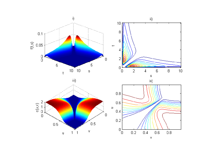
Figure 2 shows the joint pdf of the first hitting times of a standard Brownian motion through two constant boundaries b=βˆ’a=1π‘π‘Ž1b=-a=1 and the corresponding copula together with the contour lines. Figures 3 illustrates the case of constant boundaries a=βˆ’1π‘Ž1a=-1 and b=1.5𝑏1.5b=1.5 asymmetric with respect to x0subscriptπ‘₯0x_{0}. The asymmetry of the boundaries location determines peaks of different height. Note that the maximum of the joint density have inverted height in the corresponding copula.

Furthermore the Laplace transforms of gaλ​(x0)superscriptsubscriptπ‘”π‘Žπœ†subscriptπ‘₯0g_{a}^{\lambda}(x_{0}) and gbλ​(x0)superscriptsubscriptπ‘”π‘πœ†subscriptπ‘₯0g_{b}^{\lambda}(x_{0}) can be found in [8] or applying Corollary 3.7.

Remark 5.1

The stability of the algorithms introduced in Section 4, already proved by Theorem 4.2, is confirmed by the standard Brownian motion case where the pdf’s ga​(t|x0,t0)subscriptπ‘”π‘Žconditional𝑑subscriptπ‘₯0subscript𝑑0g_{a}(t|x_{0},t_{0}) and gb​(t|x0,t0)subscript𝑔𝑏conditional𝑑subscriptπ‘₯0subscript𝑑0g_{b}(t|x_{0},t_{0}) are available in closed form. We apply the algorithms to the standard Brownian motion with constant boundaries a=βˆ’1π‘Ž1a=-1 and b=2𝑏2b=2 with discretization step h=0.01β„Ž0.01h=0.01 and we compare the results with the closed form densities (6) with the series truncated to N=103𝑁superscript103N=10^{3} steps. The inversion of the Laplace transform with the Euler method gives a mean square deviation M​S​Ea=6.02β‹…10βˆ’19𝑀𝑆subscriptπΈπ‘Žβ‹…6.02superscript1019MSE_{a}=6.02\cdot 10^{-19} and M​S​Eb=9.83β‹…10βˆ’20𝑀𝑆subscript𝐸𝑏⋅9.83superscript1020MSE_{b}=9.83\cdot 10^{-20}. The numerical algorithm gives a mean square deviation M​S​Ea=3.23β‹…10βˆ’6𝑀𝑆subscriptπΈπ‘Žβ‹…3.23superscript106MSE_{a}=3.23\cdot 10^{-6} and M​S​Eb=5.11β‹…10βˆ’8𝑀𝑆subscript𝐸𝑏⋅5.11superscript108MSE_{b}=5.11\cdot 10^{-8}. It confirms the reliability of the new algorithm. The higher precision of the Laplace inversion with respect to the numerical method is determined by the simple expression of the involved Laplace transforms. However we cannot infer an analogous property for the other diffusions.

Remark 5.2

The extension of the above results to a Brownian motion with diffusion coefficient Οƒβ‰ 1𝜎1\sigma\neq 1 is straightforward. Indeed, a Brownian motion with diffusion coefficient ΟƒπœŽ\sigma can be transformed in a standard Brownian motion via the space transformation x=xβ€²/Οƒπ‘₯superscriptπ‘₯β€²πœŽx=x^{\prime}/\sigma and the boundaries aπ‘Ža and b𝑏b becomes a/Οƒπ‘ŽπœŽa/\sigma and b/Οƒπ‘πœŽb/\sigma respectively. When ΞΌ>0πœ‡0\mu>0 and a​(0)<x0<b​(0)π‘Ž0subscriptπ‘₯0𝑏0a(0)<x_{0}<b(0) one can determine gb​(t|x0,t0)subscript𝑔𝑏conditional𝑑subscriptπ‘₯0subscript𝑑0g_{b}(t|x_{0},t_{0}). In this case the crossing of the boundary a​(t)π‘Žπ‘‘a(t) is not a sure event and the study of ga​(t|x0,t0)subscriptπ‘”π‘Žconditional𝑑subscriptπ‘₯0subscript𝑑0g_{a}(t|x_{0},t_{0}) requests a suitable normalization. Similarly the case of ΞΌ<0πœ‡0\mu<0 and a​(0)<x0<b​(0)π‘Ž0subscriptπ‘₯0𝑏0a(0)<x_{0}<b(0) is analogous interchanging the role of the two boundaries.

Remark 5.3

Indicating with CTa,TbΟƒsubscriptsuperscript𝐢𝜎subscriptπ‘‡π‘Žsubscript𝑇𝑏C^{\sigma}_{T_{a},T_{b}} the copula of (Ta,Tb)subscriptπ‘‡π‘Žsubscript𝑇𝑏(T_{a},T_{b}) for a Brownian motion with diffusion coefficient ΟƒπœŽ\sigma and with CTa,Tbsubscript𝐢subscriptπ‘‡π‘Žsubscript𝑇𝑏C_{T_{a},T_{b}} the copula in the case Οƒ=1𝜎1\sigma=1, recalling the transformation x=xβ€²/Οƒπ‘₯superscriptπ‘₯β€²πœŽx=x^{\prime}/\sigma, the relationship CTa,TbΟƒ=CTa/Οƒ,Tb/Οƒsubscriptsuperscript𝐢𝜎subscriptπ‘‡π‘Žsubscript𝑇𝑏subscript𝐢subscriptπ‘‡π‘ŽπœŽsubscriptπ‘‡π‘πœŽC^{\sigma}_{T_{a},T_{b}}=C_{T_{a/\sigma},T_{b/\sigma}} holds. Geometric Brownian motion can be obtained by a standard Brownian motion via the space transformation xβ€²=exp⁑(σ​x)superscriptπ‘₯β€²πœŽπ‘₯x^{\prime}=\exp(\sigma x). The corresponding copula, CTa,TbG​B​Msubscriptsuperscript𝐢𝐺𝐡𝑀subscriptπ‘‡π‘Žsubscript𝑇𝑏C^{GBM}_{T_{a},T_{b}}, is related with the copula of the standard Brownian motion through CTa,TbG​B​M=CTln⁑a/Οƒ,Tln⁑a/Οƒsubscriptsuperscript𝐢𝐺𝐡𝑀subscriptπ‘‡π‘Žsubscript𝑇𝑏subscript𝐢subscriptπ‘‡π‘ŽπœŽsubscriptπ‘‡π‘ŽπœŽC^{GBM}_{T_{a},T_{b}}=C_{T_{\ln a/\sigma},T_{\ln a/\sigma}}.

The more general transformation xβ€²=exp⁑(μ​t+σ​x)superscriptπ‘₯β€²πœ‡π‘‘πœŽπ‘₯x^{\prime}=\exp(\mu t+\sigma x) is not interesting from the point of view of the exit times from a strip because it corresponds to transform the process into a Brownian motion with drift that has not a sure crossing, as stated in Remark 5.2.
Refer to caption
Figure 2: First hitting times of a Brownian motion through two constant boundaries b=βˆ’a=1π‘π‘Ž1b=-a=1: i) Joint pdf ii) Contour lines of the joint pdf iii) Density of the copula iv) Contour lines of the density of the copula.
Refer to caption
Figure 3: First hitting times of a Brownian motion through two constant boundaries a=βˆ’1π‘Ž1a=-1 and b=1.5𝑏1.5b=1.5: i) Joint pdf ii) Contour lines of the joint pdf iii) Density of the copula iv) Contour lines of the density of the copula.

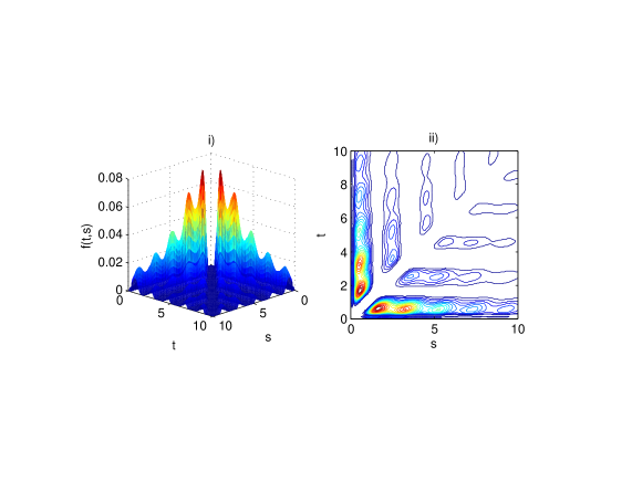
As a further example we consider a standard Brownian motion with the following boundaries b​(t)=1+0.1​cos⁑(π​t)𝑏𝑑10.1πœ‹π‘‘b(t)=1+0.1\cos(\pi t) and a​(t)=βˆ’1+0.1​cos⁑(π​t+Ο€)π‘Žπ‘‘10.1πœ‹π‘‘πœ‹a(t)=-1+0.1\cos(\pi t+\pi). Since the boundaries are time dependent, Laplace transform inversions cannot be applied. Figure 4 shows the joint pdf of the first hitting times and the corresponding contour lines obtained with the proposed numerical algorithm.
Refer to caption
Figure 4: First hitting times of a Brownian motion through two time dependent boundaries b​(t)=1+0.1​cos⁑(π​t)𝑏𝑑10.1πœ‹π‘‘b(t)=1+0.1\cos(\pi t) and a​(t)=βˆ’1+0.1​cos⁑(π​t+Ο€)π‘Žπ‘‘10.1πœ‹π‘‘πœ‹a(t)=-1+0.1\cos(\pi t+\pi): i) Joint pdf ii) Contour lines of the joint pdf .

5.2 Ornstein Uhlenbeck Process

Consider as a further example the Ornstein Uhlenbeck process, described by the stochastic differential equation

d​X​(t)𝑑𝑋𝑑\displaystyle dX(t) =\displaystyle= (βˆ’X​(t)ΞΈ+ΞΌ)​d​t+σ​d​Wtπ‘‹π‘‘πœƒπœ‡π‘‘π‘‘πœŽπ‘‘subscriptπ‘Šπ‘‘\displaystyle\left(-\frac{X(t)}{\theta}+\mu\right)dt+\sigma dW_{t} (43)
X​(t0)𝑋subscript𝑑0\displaystyle X(t_{0}) =\displaystyle= x0.subscriptπ‘₯0\displaystyle x_{0}. (44)

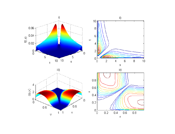
For this process representations and numerical methods are available and can be used to evaluate the first hitting time pdf fTa​(t|x0,t0)subscript𝑓subscriptπ‘‡π‘Žconditional𝑑subscriptπ‘₯0subscript𝑑0f_{T_{a}}(t|x_{0},t_{0}) [3, 10, 22]. On the other side, the density ga​(t|x0,t0)subscriptπ‘”π‘Žconditional𝑑subscriptπ‘₯0subscript𝑑0g_{a}(t|x_{0},t_{0}) is not known in closed form. Here we have applied classical numerical algorithms (cf. [10]) to evaluate the first hitting time pdf and the algorithms of Section 4 to compute the second. Figure 5 shows the joint pdf and the corresponding copula of the first hitting times of an Ornstein Uhlenbeck process with parameter ΞΈ=10πœƒ10\theta=10, ΞΌ=0πœ‡0\mu=0, Οƒ=1𝜎1\sigma=1 and x0=0subscriptπ‘₯00x_{0}=0 through two constant boundaries b=βˆ’a=1π‘π‘Ž1b=-a=1. Figures 6 illustrates the case of asymmetric w.r.t. x0subscriptπ‘₯0x_{0} constant boundaries a=βˆ’1π‘Ž1a=-1 and b=1.5𝑏1.5b=1.5. Note that x0subscriptπ‘₯0x_{0} represents the symmetry axis of the Ornstein Uhlenbeck process. The height of the peaks of the joint density and of the copula behaves as the Brownian motion case.
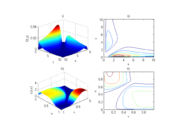
Refer to caption
Figure 5: First hitting times of an Ornstein Uhlenbeck process through two constant boundaries b=βˆ’a=1π‘π‘Ž1b=-a=1: i) Joint pdf ii) Contour lines of the joint pdf iii) Density of the copula iv) Contour lines of the density of the copula.
Refer to caption
Figure 6: First hitting times of an Ornstein Uhlenbeck process through two constant boundaries a=βˆ’1π‘Ž1a=-1 and b=1.5𝑏1.5b=1.5: i) Joint pdf ii) Contour lines of the joint pdf iii) Density of the copula iv) Contour lines of the density of the copula.

The Laplace transforms gaλ​(x0)superscriptsubscriptπ‘”π‘Žπœ†subscriptπ‘₯0g_{a}^{\lambda}(x_{0}) and gbλ​(x0)superscriptsubscriptπ‘”π‘πœ†subscriptπ‘₯0g_{b}^{\lambda}(x_{0}) for the OU process can be found in [8]. However the presence of the parabolic cylinder functions in their expression discourage their numerical inversion.

\acks

We are grateful to an anonymous referee for his interesting and constructive comments to improve the paper. Work supported in part by University of Torino Grant 2012 β€œStochastic Processes and their Applications”and by project A.M.A.L.F.I. - Advanced Methodologies for the AnaLysis and management of the Future Internet (UniversitΓ  di Torino/Compagnia di San Paolo).

References

  • [1] Abate, J. (1995) Numerical inversion of Laplace transforms of probability distributions. ORSA Journal on Computing 7, 36–43.
  • [2] Albano, G. and Giorno V. (2006) A stochastic model in tumor growth. J Theor. Biol. 242, 329–336.
  • [3] Alili, L., Patie P. and Pedersen, J.L. (2005) Representations of the First Hitting Time Density of an Ornstein-Uhlenbeck Process. Stoch. Model. 21, 967–980.
  • [4] Arnold, L. (1974) Stochastic differential equations: Theory and Applications. Wiley-Interscience, New York.
  • [5] Bassan, B. and Spizzichino, F. (2005) Relations among univariate aging, bivariate aging and dependence for exchangeable lifetimes. J. Multivariate Anal. 93 1, 313–339.
  • [6] Bassan, B. and Spizzichino, F. (2005) Bivariate survival models with Clayton aging functions. Insurance Math. Econom. 37 1, 6–12.
  • [7] Benedetto, E., Sacerdote, L. and Zucca, C. (2013) A first passage problem for a bivariate diffusion process: numerical solution with an application to neuroscience when the process is Gauss-Markov. J. Comput. Appl. Math. 242, 41–52.
  • [8] Borodin, A.N. and Salminen, P. (2002) Handbook of Brownian Motion Facts and Formulae, 2nd edition. Birkh user, Basel.
  • [9] Buonocore, A., Giorno V., Nobile, A.G. and Ricciardi, L.M. (1990) On the two-boundary first-crossing-time problem for diffusion processes. J. Appl. Probab. 27 1, 102–114.
  • [10] Buonocore, A., Nobile, A.G. and Ricciardi, L.M. (1987) A new integral equation for the evaluation of first-passage-time probability densities. Adv. in Appl. Probab. 19 4, 784–800.
  • [11] Capocelli, R.M., and Ricciardi L.M. (1976) On the transformation of diffusion processes into the Feller process. Math. Biosciences 29, 219-234.
  • [12] Di Crescenzo A., Giorno V., Nobile A.G.and Ricciardi, L.M. (1995) On a symmetry-based constructive approach to probability densities for two-dimensional diffusion processes. J. Appl. Probab. 32 2, 316–336.
  • [13] Davydov D., and Linetsky, V. (2003) Pricing Options on Scalar Diffusions: An Eigenfunction Expansion Approach. Oper. Res. 51 2, 185–209.
  • [14] Galleani, L., Sacerdote, L., Tavella P. and Zucca, C. (2003) A mathematical model for the atomic clock error. Metrologia 40 4, S257–S264.
  • [15] Giorno V., Nobile A.G. and Ricciardi, L.M. (2011) On the densities of certain bounded diffusion processes. Ricerche mat. 60, 89–124.
  • [16] Giorno V., Nobile A.G., Ricciardi, L.M. and Sacerdote, L. (1986) Some remarks on the Rayleigh process. J. Appl. Prob. 23, 398–408.
  • [17] Giraudo, M.T. and Sacerdote, L. (1999) An improved technique for the simulation of first passage times for diffusion processes. Commun. Statist. Simul. 28 4, 1135–1163.
  • [18] Giraudo, M.T. and Sacerdote, L. (2013) Leaky Integrate and Fire models: a review on mathematicals methods and their applications. Lecture Notes in Mathematics 2058 4, 95–142.
  • [19] Giraudo, M.T., Sacerdote, L. and Zucca, C. (2001) Evaluation of first passage times of diffusion processes through boundaries by means of a totally simulative algorithm. Meth.Comp. Appl. Prob. 3 2, 215–231.
  • [20] Ito, K. and McKean, K.P. (1974). Diffusion Processes and Their Sample Paths. Springer.
  • [21] Lapidus, L. and Pinder, G.F. (1999). Numerical Solution of Partial Differential Equations in Science and Engineering. Wiley.
  • [22] Linetsky, V. (2004) Computing hitting time densities for CIR and OU diffusions: applications to mean-reverting models J. Comput. Finance 7 406, 1–22.
  • [23] Linz, P. (1985). Analytical and numerical methods for Volterra equations. SIAM, Philadelphia.
  • [24] Nelsen, R.B. (1999) An introduction to copulas, Lecture notes in Statistics 139, Springer, New York.
  • [25] Novikov, A., Frishling, V. and Kordzakhia, N. (1999) Approximations of Boundary Crossing Probabilities for a Brownian Motion. J. Appl. Prob. 36, 1019–1030.
  • [26] Oakes, D. (1989). Bivariate survival models induced by frailties. J. Amer. Statist. Assoc. 84 406, 487–493.
  • [27] Orsingher, E. and Beghin, L. (2006) ProbabilitΓ  e modelli aleatori. Aracne Editrice, Roma.
  • [28] Panfilo, G., Tavella, P. and Zucca, C. (2004) How long does a clock error remain inside two threshold barriers? An evaluation by means of stochastic processes. Proc. European Frequency and Time Forum, Guilford.
  • [29] Peskir, G. (2002). Limit at zero of the Brownian first-passage density. Probab. Theory Related Fields. 124, 100–111.
  • [30] Ricciardi, L.M. (1976) On the transformation of diffusion processes into the Wiener process. J. Math. Analysis Appl. 54, 185-199.
  • [31] Ricciardi, L.M. (1977) Diffusion Processes and Related Topics in Biology, Lecture Notes in Biomathematics, Vol. 14. Springer Verlag, Berlin.
  • [32] Ricciardi, L.M., Di Crescenzo, A., Giorno V. and Nobile A.G. (1999) An outline of theoretical and algorithmic approaches to first passage time problems with applications to biological modeling. Math. Japonica 50 2, 247–322.
  • [33] Ricciardi, L.M. and Sacerdote L. (1987) On the probability densities of an Ornstein-Uhlenbeck process with a reflecting boundary. J. Appl. Prob. 24, 355–369.
  • [34] Ricciardi, L.M., Sacerdote L. and Sato, S. (1984) On an integral equation for first-passage-time probability densities. J. Appl. Prob. 21 2, 302–314.
  • [35] Ricciardi, L.M. and Sato, S. (1990) Diffusion processes and first-passage-time problems. In: L.M. Ricciardi (Ed.), Lectures in Applied Mathematics and Informatics. Manchester Univ. Press., Manchester.
  • [36] Smith G.D. (1978) Numerical Solution of Partial Differential Equations: Finite Difference Methods. Oxford Univ. Press.
  • [37] Smith P.L. (2000) Stochastic dynamic models of response time and accuracy: A foundational primer. J. Math. Psychol. 44 3, 408–463.
  • [38] Spizzichino, F. (2001) Subjective probability models for lifetimes. Chapman and Hall/CRC. Boca Raton, Fl.
  • [39] Tricomi, F.G. (1957) Integral equations. Interscience, New York.
  • [40] Van Loan C.F. (1992) Computational Frameworks for the Fast Fourier Transform. Siam, Philadelphia.
  • [41] Zucca, C. and Sacerdote, L. (2009) On the inverse first-passage-time problem for a Wiener process. Ann. Appl. Probab. 19 4, 1319–1346.