Microscopic Analysis of Resonant Inelastic X-Ray Scattering in Orbital-Ordered KCuF₃

Abstract

We analyze resonant inelastic x-ray scattering (RIXS) at the Cu $K$ edge in a typical orbital-ordered compound KCuF₃ on the basis of a microscopic theory. Spectral shape and its dependence on polarization direction and momentum transfer of photons are explained consistently with experimental data within our microscopic calculation. According to our microscopic orbital-resolving analysis, high-energy spectral weights (above 5 eV) originate from charge-transfer excitations related to the Cu-$d\gamma$ orbitals, while the low-energy weights (below 2 eV) originate from the $d$-$d$ orbital excitations among the five Cu-$d$ orbitals. We assign specifically the RIXS weights to microscopic orbital-excitation processes, beyond the previous phenomenological assignment based on symmetry properties.

1 Introduction

Resonant inelastic x-ray scattering (RIXS) is growing up to be a powerful method of measuring elementary excitations in solids [1]. Among RIXS phenomena, RIXS at the transition-metal $K$ edges attracts much interest, because it provides to us a unique technique to observe charge and orbital excitations in strongly correlated $d$ electrons of transition-metal compounds  [2, 3, 4, 5, 6, 7]. Here we illustrate the RIXS process at the transition-metal $K$ edge: firstly, an incident photon with the energy tuned to the transition-metal $K$ edge is resonantly absorbed to promote an inner-shell $1s$ electron to the $4p$ conduction bands (in the case of 3$d$ transition-metal compounds), following the dipole-transition rule, and in the intermediate state a hole is created at the local $1s$ orbital. The created $1s$ hole plays a role of a local scattering body for the electrons near the Fermi level. In other words, electrons near the Fermi level are excited to screen the created $1s$ hole. Before the excitation near the Fermi level damps, the initially excited $4p$ electron goes back to the $1s$ state to fill the $1s$ hole, with emitting a photon. Following the energy-momentum conservation law, the emitted photon should have energy and momentum which differ from those of the incident photon by the amount of energy and momentum spent to excite the electrons near the Fermi level. Here we should note that not all of the electrons near the Fermi level are evenly excited in the intermediate and final states: electrons only weakly interacting with the $1s$ hole are not strongly excited. On the other hand, electrons strongly interacting with the $1s$ hole can be strongly excited. Transition-metal $d$ electrons ($3d$ electrons in the cases of 3$d$ transition-metal compounds) are relatively localized in space, and therefore the Coulomb interaction between the $1s$ and $d$ orbitals is expected to be strong. Thus, RIXS at the $K$ edge in transition-metal compounds enables us to observe selectively the excitations of strongly correlated $d$ electrons.

RIXS in transition-metal compounds has been studied intensively also from theoretical sides. This is partly because RIXS is a relatively difficult phenomenon to interpret without intricate theoretical considerations. RIXS not only involves complex intermediate excitation processes but is subject to strong electron correlations, as easily understood. Thus, RIXS has provided good opportunities of applying various theoretical approaches, e.g., numerical diagonalization for finite-size clusters[8], many-body perturbation theory [9, 10], dynamical mean-field theory [11] and so on [12, 13]. Among several theoretical studies, we previously derived a useful formula to calculate RIXS spectra by taking account of the above mentioned RIXS process within the Keldysh perturbative formalism [9, 10, 14], and analyzed RIXS spectral properties for many transition-metal compounds [9, 10, 14, 15, 16, 17]. In our previous works [9, 10, 14] and most of others’ works, the excited $4p$ electron has been considered to be a ‘spectator’ [18]. In fact, the electronic structure for the $4p$ bands has been highly simplified or treated only crudely in most of previous works  [12, 8, 9, 10, 13].

Recently, Ishii and collaborators measured RIXS at the Cu $K$ edge in a typical orbital-ordered compound KCuF₃ [6]. They observed that the low-energy RIXS weights show notable characteristic dependence on polarization direction of photons, while they did not observed any notable momentum dependence. They attributed the observed low-energy features to possible $d$-$d$ excitation processes phenomenologically on the basis of symmetry properties. According to the dipole-transition rule, the polarization direction is closely related to the excited $4p$ state in the intermediate state of RIXS. Therefore, such notable polarization dependence suggests strongly that the $4p$ electron plays a much more important role than a ‘spectator’.

The aim of our present study is to analyze theoretically spectral shape and its dependence on the polarization direction and momentum transfer of photons within a microscopic calculation. In addition, we elucidate microscopically relevant orbital-excitation processes in RIXS of KCuF₃, by introducing our new method of orbital-resolving analysis. The present article is constructed as follows: In § 2, we present our Hamiltonian and perturbative formulation for RIXS intensity. We also define orbital-resolved RIXS spectra. To describe the electronic structure of KCuF₃ precisely, we use first-principles band structure calculation, and determine the antiferromagnetic ground state within the Hartree-Fock (HF) approximation. Electron correlations in the intermediate states are treated within the random-phase approximation (RPA). In § 3, we present numerical results on RIXS spectra and their dependences on polarization and momentum transfer of photons. The origin of each spectral weight is microscopically analyzed in detail by resolving orbital-excitation processes. In § 4, some discussions and remarks on our formulation and results are given. In § 5, the article is concluded with summary.

2 Formulation of RIXS

To discuss the RIXS process microscopically, we consider the following form of Hamiltonian:

$$H=H_{n.f.}+H_{1s}+H_{1s-d}+H_{x},$$ (1)

where $H_{1s}$ and $H_{x}$ describe the inner-shell $1s$ electrons and the dipole-transition by x-rays, respectively. $H_{n.f.}$ describes the correlated electrons near the Fermi level. $H_{1s-d}$ is the Coulomb interaction between $1s$ and transition-metal $d$ electrons. For $1s$ electrons, we take completely localized $1s$ orbitals at each transition-metal site:

$$H_{1s}=\sum_{i}^{\rm t.m.}\sum_{\sigma}\varepsilon_{1s}(\mib{r}_{i})s_{i\sigma}^{{\dagger}}s_{i\sigma}=\sum_{\mib{k}\sigma}\varepsilon_{1s}s_{{\mib k}\sigma}^{{\dagger}}s_{{\mib k}\sigma},$$ (2)

where $\varepsilon_{1s}(\mib{r}_{i})\equiv\varepsilon_{1s}$ is the one-particle energy of the $1s$ state, $s_{i\sigma}^{{\dagger}}$ and $s_{i\sigma}$ are the creation and annihilation operators of $1s$ electrons with spin $\sigma$ at transition-metal site $i$, respectively. ‘$\rm{t.m.}$’ in the summation with respect to $i$ means summing only over transition-metal sites. $s_{{\mib k}\sigma}(s_{{\mib k}\sigma}^{{\dagger}})$ is the momentum representation of $s_{i\sigma}(s_{i\sigma}^{{\dagger}})$. $H_{x}$ describes resonant $1s$-$4p$ dipole transition induced by x-rays:

$$H_{x}=\sum_{\mib{k},\mib{q}}\sum_{\mu}^{xyz}\sum_{\sigma}w_{\mu}({\mib q},{\mib e})\alpha_{\mib{q}\mib{e}}p_{{\mib k}+{\mib q}\mu\sigma}^{{\dagger}}s_{{\mib k}\sigma}+h.c.,$$ (3)

where $p_{{\mib k}\mu\sigma}^{{\dagger}}$ is the creation operator of transition-metal $4p_{\mu}$ electron ($\mu=x,y,z$), and $\alpha_{\mib{q}\mib{e}}$ is the annihilation operator of a photon with momentum $\mib{q}$ and polarization $\mib{e}$. The summation in $\mu$ with ‘$xyz$’ at the top means that $\mu$ takes $x$, $y$ or $z$. We assume the matrix elements of $w_{\mu}(\mib{q},\mib{e})$ are given in the form:

$$w_{\mu}(\mib{q},\mib{e})=-\frac{e}{m}\sqrt{\frac{2\pi}{|\mib{q}|}}\mib{e}\cdot\langle 4p_{\mu}|\mib{p}|1s\rangle\propto\mib{e}\cdot\mib{e}_{\mu},$$ (4)

in natural units ($c=\hbar=1$). $\mib{e}_{\mu}$’s are the orthonormal basis vectors. $H_{1s-d}$ is given by

$$H_{1s-d}=\sum_{i}^{\rm t.m.}\sum_{\sigma\sigma^{\prime}}V_{1s-d}(\mib{r}_{i})s_{i\sigma}^{{\dagger}}d_{i\sigma^{\prime}}^{{\dagger}}d_{i\sigma^{\prime}}s_{i\sigma},$$ (5)

where $V_{1s-d}(\mib{r}_{i})$ is the so-called core-hole potential at transition-metal site $\mib{r}_{i}$. In the present study on KCuF₃, we take $V_{1s-d}(\mib{r}_{i})\equiv V_{1s-d}=9$ eV at Cu sites.

To prepare the Hamiltonian part $H_{n.f.}$, firstly we perform first-principles band structure calculation assuming the paramagnetic state [19]. The orbital-ordered state is schematically represented in Fig. 1. To express the electronic orbital bases and scattering geometry, we throughout take the coordinate system where the principal axes of the pseudo-cube constructed by Cu sites are parallel along the cartesian axes (see Fig 1).

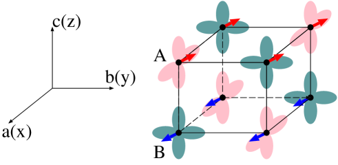
Figure 1: (Color online) Schematic representation of the orbital-ordered state of KCuF₃ [20, 21, 22, 23, 24]. Cu atoms are placed on the corners of the pseudo-cubic cell (K and F sites are not shown explicitly). There are two kinds of Cu sites, depending on the orbital state: At A sites, Cu-$d_{x^{2}-z^{2}}$ states are filled almost by one half with electrons, while at B sites Cu-$d_{y^{2}-z^{2}}$ states are. Thick arrows represent the direction of the spin moment at each Cu site. The spin moments are parallel along the $ab$ plane in the antiferromagnetic ground state.

We assume the so-called ‘a-type’ structure (space group: $D_{4h}^{18}-I4/mcm$) [25, 26], and use the structure parameters given in Ref. References. Then we perform tight-binding fitting to the obtained energy bands near the Fermi level by using the wannier90 code [28, 29], where we take $p$ and $d$ orbitals at K sites, $s$, $p$ and $d$ orbitals at Cu sites, and $p$ orbitals at F sites. Here we should interpret these $s$ orbitals at Cu sites as $4s$ orbitals, and not confuse with the $1s$ orbitals. Thus we include 52 localized Wannier states in the unit cell, because there are two K, two Cu and six F sites in the unit cell. Concerning the $d$ orbitals at Cu sites, we take $d(xy,yz,xz,x^{2}-z^{2},3y^{2}-r^{2})$ at A sites and $d(xy,yz,xz,y^{2}-z^{2},3x^{2}-r^{2})$ at B sites, where the orbital bases are defined following the coordinate axes in Fig. 1. Thus we obtain a tight-binding model to fit the 52 bands in the energy window from $-8$ eV to 20 eV with respect to the Fermi energy. The reason why we choose those 52 localized orbitals is that those orbitals occupy the main part of the density of states in this energy window, according to the band structure calculation. We take about 14000 hoppings $t_{\ell\ell^{\prime}}({\mib r})$ with ${\mib r}$ up to at most 10 lattice units. Adding the on-site Coulomb interaction part, we have the Hamiltonian part $H_{n.f.}$ in the following form:

$$H_{n.f.}=\sum_{ii^{\prime}}\sum_{\ell\ell^{\prime}}\sum_{\sigma}t_{\ell\ell^{\prime}}({\mib r}_{i}-\mib{r}_{i^{\prime}})a_{i\ell\sigma}^{{\dagger}}a_{i^{\prime}\ell^{\prime}\sigma}+\frac{1}{2}\sum_{i}^{\rm t.m.}\sum_{\ell_{1\sim 4}}^{@\mib{r}_{i}}\sum_{\sigma\sigma^{\prime}}I_{\ell_{1}\ell_{2};\ell_{3}\ell_{4}}(\mib{r}_{i})a_{i\ell_{1}\sigma}^{{\dagger}}a_{i\ell_{2}\sigma^{\prime}}^{{\dagger}}a_{i\ell_{3}\sigma^{\prime}}a_{i\ell_{4}\sigma},$$ (6)

where $a_{i\ell\sigma}^{{\dagger}}$ and $a_{i\ell\sigma}$ are the electron creation and annihilation operators for orbital $\ell$ with spin $\sigma$ at site $i$. $I_{\ell_{1}\ell_{2};\ell_{3}\ell_{4}}(\mib{r}_{i})\equiv I_{\ell_{1}\ell_{2};\ell_{3}\ell_{4}}$ is the on-site Coulomb integral at transition-metal (i.e., Cu) sites. In the summation with respect to $\ell_{n}$, ‘$@\mib{r}_{i}$’ at the top means orbital $\ell_{n}$ should be placed on the site $\mib{r}_{i}$. One-particle energy at orbital $\ell$ is given by $\varepsilon_{\ell}\equiv t_{\ell\ell}(\mib{r}=0)$. We modify the one-particle energy $\varepsilon_{\ell}$ for Cu-$d$ orbitals, to obtain a realistic level scheme of the local Cu-$d$ orbitals, as explained in Appendix. Hereafter we use the following convention: if $\ell$ denotes $d$ orbital (e.g., $\ell=xy$), then $a_{i\ell\sigma}\equiv d_{i\ell\sigma}$, if $\ell$ denotes $p$ orbital (e.g., $\ell=x$), then $a_{i\ell\sigma}\equiv p_{i\ell\sigma}$, and so on. $a_{i\ell\sigma}$ contains also the annihilation operators at K and F sites. However, we expect that the above convention does not cause any confusion among the operators for K-$p$, Cu-$p$ and F-$p$ orbitals, or between the operators for K-$d$ and Cu-$d$ orbitals, because the operators for orbitals at K and F sites do not appear explicitly in the present article. Here we introduce the values of on-site Coulomb interaction $I_{\ell_{1}\ell_{2};\ell_{3}\ell_{4}}$ at each Cu site in the form of Slater-Condon integrals (see Ref. References for the definition of Slater-Condon integrals and their relation to $I_{\ell_{1}\ell_{2};\ell_{3}\ell_{4}}$): $F_{dd}^{0}=10.5$ eV, $F_{dd}^{2}=12$ eV, $F_{dd}^{4}=8$ eV. These values of $F_{dd}^{2}$ and $F_{dd}^{4}$ are similar to those determined for copper oxides in Ref. References (11.5 eV and 7.4 eV, respectively, there). Our choice of these Coulomb integrals corresponds approximately to $U\sim 11$-12 eV, $U^{\prime}\sim 10$ eV, and $J\sim 1$ eV, where $U$, $U^{\prime}$ and $J$ are the intra-orbital, inter-orbital and Hund’s couplings, respectively. This value of $U$ is similar to that in our previous study for copper oxides [9, 10]. In addition, we take account of the Coulomb interaction between the $4p$ and $d$ electrons: $F_{pd}^{0}=3$ eV, $F_{pd}^{2}=3$ eV. For $H_{n.f.}$, we determine the antiferromagnetic ground state within the HF approximation (see Appendix about details of HF calculation).

RIXS intensity can be obtained by calculating the number of photons generated in different states from the incident-photon state per unit time, as shown by Nozières and Abrahams [32]. To do this, we employ Keldysh perturbation theory as in Ref. References and our previous works [9, 10, 14]. The RIXS intensity is generally expressed by the diagram (I) in Fig. 2, if assuming that only a single electron-hole pair remains in the final state.

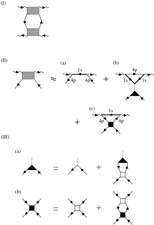
Figure 2: (I) RIXS intensity represented within the Keldysh perturbative formulation. The wavy lines and shaded rectangular represent the photon propagators and electron scattering vertex function $F(q,q^{\prime})$, respectively. A pair of oriented solid lines represent the off-diagonal elements of the Keldysh Green’s function, and connect the upper normally-time-ordered and lower reversely-time-ordered branches. (II) Approximate expansion for the scattering vertex function $F(q,q^{\prime})$: (a) $F^{(0)}(q,q^{\prime})$ for ‘0th-order process’ (fluorescence), (b) $F^{(s)}(q,q^{\prime})$ for ‘$s$-process’, (c) $F^{(p)}(q,q^{\prime})$ for ‘$p$-process’. The filled triangle and square are the three-point and four-point vertex functions to be renormalized by electron correlations, respectively. In (b), the dashed line represents the core-hole potential $V_{1s-d}$. Thick solid lines represent the propagator of the inner-shell $1s$ electrons. (III) RPA diagrams for the three-point and four-point vertex functions ((a) and (b), respectively), where empty squares represent the antisymmetrized bare Coulomb interaction $\Gamma^{(0)}$ among the $d$ and $4p$ electrons at transition-metal sites.

The analytic expression of RIXS intensity is obtained from the diagram (I) of Fig. 2 as:

$$W(q,q^{\prime}) = \frac{1}{N}\sum_{\mib{k}_{1}}\int_{-\infty}^{\infty}\frac{d\omega_{1}}{2\pi}\sum_{j_{1}j_{2}}G_{j_{1}}^{+}(k_{1})G_{j_{2}}^{-}(k_{1}+Q)$$ (7)

$$\times\biggl{|}\sum_{\mu\mu^{\prime}}^{xyz}w_{\mu}(\mib{q},\mib{e})w_{\mu^{\prime}}(\mib{q}^{\prime},\mib{e}^{\prime})F_{\mu\mu^{\prime};j_{1}j_{2}}(k_{1};q,q^{\prime})\biggr{|}^{2},$$

where $G_{j}^{\pm}(k)$ is the Keldysh Green’s function [33], $j_{1,2}$ are indices for the diagonalized bands, and $k_{1}=(\omega_{1},\mib{k}_{1})$. $q$ and $q^{\prime}$ are the four-momenta of the incident and emitted photons, respectively: $q=(\omega,\mib{q})$, $q^{\prime}=(\omega^{\prime},\mib{q}^{\prime})$. $Q$ is the energy and momentum loss of the photon: $Q=q-q^{\prime}=(\omega-\omega^{\prime},\mib{q}-\mib{q}^{\prime})\equiv(\Omega,\mib{Q})$. $F_{\mu\mu^{\prime};j_{1}j_{2}}(k_{1};q,q^{\prime})$ is the scattering vertex function expressed using only the usual causal electron Green’s functions and electron-electron interaction. At this stage, we omit $\omega_{1}$ dependence of $F_{\mu\mu^{\prime};j_{1}j_{2}}(k_{1};q,q^{\prime})$, i.e., $F_{\mu\mu^{\prime};j_{1}j_{2}}(k_{1};q,q^{\prime})=F_{\mu\mu^{\prime};j_{1}j_{2}}(\mib{k}_{1};q,q^{\prime})$, because it is justified within the following approximation for $F_{\mu\mu^{\prime};j_{1}j_{2}}(k_{1};q,q^{\prime})$. Within the HF approximation, the Green’s functions $G_{j}^{\pm}(k)$ are given by

$$G_{j}^{+}(k_{1}) = 2\pi in_{j}(\mib{k}_{1})\delta(\omega_{1}-E_{j}(\mib{k}_{1})),$$ (8)

$$G_{j}^{-}(k_{1}) = -2\pi i[1-n_{j}(\mib{k}_{1})]\delta(\omega_{1}-E_{j}(\mib{k}_{1})),$$ (9)

where $E_{j}(\mib{k}_{1})$ is the energy of diagonalized band $j$, and $n_{j}(\mib{k}_{1})$ is the electron occupation density at momentum $\mib{k}_{1}$ in band $j$: $n_{j}(\mib{k}_{1})=1$ for $E_{j}(\mib{k}_{1})<0$ and $n_{j}(\mib{k}_{1})=0$ for $E_{j}(\mib{k}_{1})>0$. Substituting eqs. (8) and (9) into eq. (7), we have

$$W(q,q^{\prime}) = \frac{2\pi}{N}\sum_{\mib{k}_{1}}\sum_{j_{1}j_{2}}n_{j_{1}}(\mib{k}_{1})[1-n_{j_{2}}(\mib{k}_{1}+\mib{Q})]\delta(\Omega+E_{j_{1}}(\mib{k}_{1})-E_{j_{2}}(\mib{k}_{1}+\mib{Q}))$$ (10)

$$\times\biggl{|}\sum_{\mu\mu^{\prime}}^{xyz}w_{\mu}(\mib{q},\mib{e})w_{\mu^{\prime}}(\mib{q}^{\prime},\mib{e}^{\prime})F_{\mu\mu^{\prime};j_{1}j_{2}}(\mib{k}_{1};q,q^{\prime})\biggr{|}^{2}.$$

For calculation of $F_{\mu\mu^{\prime};j_{1}j_{2}}(\mib{k}_{1};q,q^{\prime})$, we use perturbation expansion with respect to electron-electron interactions. There are three major contributions to $F_{\mu\mu^{\prime};j_{1}j_{2}}(\mib{k}_{1};q,q^{\prime})$. The first is the zeroth-order term represented by the diagram (II)-(a) in Fig. 2. This diagram presents a main contribution to the fluorescence yield. We refer to this contribution as ‘0th-order process’. The second originates from the screening process of the $1s$ core hole. Within the Born approximation with respect to the core-hole potential $V_{1s-d}$, this process is expressed by the diagram (II)-(b) in Fig. 2. We refer to this contribution as ‘$s$-screening process’ or ‘$s$-process’. The $s$-screening process has been included in our previous works [9, 10]. The third describes the screening process of the excited $4p$ electron. Within the Born approximation (or equivalently the linear response approximation with respect to the potential polarizing the transition-metal $d$-electrons), this contribution is expressed by the diagram (II)-(c) in Fig. 2. We refer to this contribution as ‘$p$-screening process’ or ‘$p$-process’. Of course, in higher-order contributions, more complex diagrams can appear, which cannot simply be classified to ‘$s$-screening process’ or ‘$p$-screening process’. Nevertheless, this classification turns out to be convenient for microscopic analysis of RIXS spectra. Thus, we obtain the following approximate expression for the scattering vertex function:

$$F_{\mu\mu^{\prime};j_{1}j_{2}}(\mib{k}_{1};q,q^{\prime}) = F^{(0)}_{\mu\mu^{\prime};j_{1}j_{2}}(\mib{k}_{1};q,q^{\prime})$$ (11)

$$-\sum_{\zeta_{1}\zeta_{2}}u_{\zeta_{2},j_{2}}^{*}(\mib{k}_{1}+\mib{Q})u_{\zeta_{1},j_{1}}(\mib{k}_{1})[F^{(s)}_{\mu\mu^{\prime};\zeta_{1}\zeta_{2}}(q,q^{\prime})+F^{(p)}_{\mu\mu^{\prime};\zeta_{1}\zeta_{2}}(q,q^{\prime})],$$

where $u_{\zeta,j}(\mib{k})$ is the diagonalization matrix of the HF Hamiltonian given by eq. (28). $\zeta_{n}$ is orbital-spin combined index: $\zeta_{n}=(\ell_{n},\sigma_{n})$, and $\sum_{\zeta_{n}}=\sum_{\ell_{n}}\sum_{\sigma_{n}}$, where $\ell_{n}$ represents $4p$ and $d$ orbitals at transition-metal sites. Contributions from the above three processes are given by

$$F^{(0)}_{\mu\mu^{\prime};j_{1}j_{2}}(\mib{k}_{1};q,q^{\prime}) = \sum_{i}^{\rm t.m.u.}\sum_{\sigma}\frac{u_{4p_{\mu}(i)\sigma,j_{2}}^{*}(\mib{k}_{1}+\mib{Q})u_{4p_{\mu^{\prime}}(i)\sigma,j_{1}}(\mib{k}_{1})}{\omega+\tilde{\varepsilon}_{1s}(\mib{r}_{i})-E_{j_{2}}(\mib{k}_{1}+\mib{Q})},$$ (12)

$$F^{(s)}_{\mu\mu^{\prime};\zeta_{1}\zeta_{2}}(q,q^{\prime}) = \sum_{i}^{\rm t.m.u.}V_{1s-d}(\mib{r}_{i})\Lambda_{\zeta_{2}\zeta_{1}}(\mib{r}_{i};Q)$$ (13)

$$\times\sum_{j\sigma}\frac{1}{N}\sum_{\mib{k}}^{E>0}\frac{u_{4p_{\mu}(i)\sigma,j}^{*}(\mib{k})u_{4p_{\mu^{\prime}}(i)\sigma,j}(\mib{k})}{[\omega+\tilde{\varepsilon}_{1s}(\mib{r}_{i})-E_{j}(\mib{k})][\omega^{\prime}+\tilde{\varepsilon}_{1s}(\mib{r}_{i})-E_{j}(\mib{k})]},$$

$$F^{(p)}_{\mu\mu^{\prime};\zeta_{1}\zeta_{2}}(q,q^{\prime}) = \sum_{i}^{\rm t.m.u.}\sum_{\zeta_{3}\zeta_{4}}^{@\mib{r}_{i}}\Gamma_{\zeta_{2}\zeta_{4},\zeta_{3}\zeta_{1}}(Q)$$

$$\times\sum_{j_{3}j_{4}\sigma}\frac{1}{N}\sum_{\mib{k}}^{E>0}\frac{u_{\zeta_{3},j_{3}}(\mib{k}+\mib{Q})u_{4p_{\mu}(i)\sigma,j_{3}}^{*}(\mib{k}+\mib{Q})u_{\zeta_{4},j_{4}}^{*}(\mib{k})u_{4p_{\mu^{\prime}}(i)\sigma,j_{4}}(\mib{k})}{[\omega+\tilde{\varepsilon}_{1s}(\mib{r}_{i})-E_{j_{3}}(\mib{k}+\mib{Q})][\omega^{\prime}+\tilde{\varepsilon}_{1s}(\mib{r}_{i})-E_{j_{4}}(\mib{k})]},$$

where $\Lambda_{\zeta_{2}\zeta_{1}}(\mib{r}_{i};Q)$ and $\Gamma_{\zeta_{2}\zeta_{4},\zeta_{3}\zeta_{1}}(Q)$ are the three-point and four-point vertex functions, which are represented by the filled triangle and square in Fig. 2 (II) (b) and (c), respectively. $4p_{\mu}(i)\sigma$ means the $4p_{\mu}$ state at transition-metal site $\mib{r}_{i}$ with spin $\sigma$. $\tilde{\varepsilon}_{1s}(\mib{r}_{i})\equiv\varepsilon_{1s}(\mib{r}_{i})+i\Gamma_{1s}$, where $\Gamma_{1s}$ is the damping rate of the $1s$ core-hole and set to 0.8 eV in the present study. Summations in $i$ with ‘t.m.u.’ at the top means that $\mib{r}_{i}$ should be restricted only to transition-metal sites in the unit cell. ‘$E>0$’ appearing in the summation about $\mib{k}$ means restriction to the $\mib{k}$-region satisfying $E_{j}(\mib{k})>0$ in eq. (13), and to the $\mib{k}$-region satisfying both $E_{j_{3}}(\mib{k}+\mib{Q})>0$ and $E_{j_{4}}(\mib{k})>0$ in eq. (2). To obtain eq. (2), we have omitted the processes where, before the excited $4p$ electron interacts, the $1s$ core-hole annihilates with other $4p$ electrons. The omitted processes give only a behavior similar to usual fluorescence and is negligible in analysis of RIXS.

The vertex functions introduced above are renormalized by electron correlations. We take account of electron correlations within RPA. RPA for $\Lambda_{\zeta_{2}\zeta_{1}}(\mib{r}_{i};Q)$ and $\Gamma_{\zeta_{2}\zeta_{4},\zeta_{3}\zeta_{1}}(Q)$ is represented diagrammatically in Fig. 2 (III) (a) and (b), respectively. The analytic expressions for these diagrams are

$$\Lambda_{\zeta_{2}\zeta_{1}}(\mib{r}_{i};Q)=\delta_{\zeta_{1}\zeta_{2}}^{{\rm t.m.}@\mib{r}_{i}}-\sum_{\zeta_{1}^{\prime}\zeta_{2}^{\prime}}^{@\mib{r}_{i}}\sum_{\zeta_{3}^{\prime}\zeta_{4}^{\prime}}\Lambda_{\zeta_{2}^{\prime}\zeta_{1}^{\prime}}(\mib{r}_{i};Q)\chi_{\zeta_{3}^{\prime}\zeta_{2}^{\prime},\zeta_{1}^{\prime}\zeta_{4}^{\prime}}(Q)\Gamma_{\zeta_{2}\zeta_{4}^{\prime};\zeta_{3}^{\prime}\zeta_{1}}^{(0)},$$ (15)

$$\Gamma_{\zeta_{2}\zeta_{4};\zeta_{3}\zeta_{1}}(Q)=\Gamma_{\zeta_{2}\zeta_{4};\zeta_{3}\zeta_{1}}^{(0)}-\sum_{\zeta_{1}^{\prime}\zeta_{2}^{\prime}}\sum_{\zeta_{3}^{\prime}\zeta_{4}^{\prime}}\Gamma_{\zeta_{2}^{\prime}\zeta_{4};\zeta_{3}\zeta_{1}^{\prime}}(Q)\chi_{\zeta_{3}^{\prime}\zeta_{2}^{\prime},\zeta_{1}^{\prime}\zeta_{4}^{\prime}}(Q)\Gamma_{\zeta_{2}\zeta_{4}^{\prime};\zeta_{3}^{\prime}\zeta_{1}}^{(0)},$$ (16)

where $\Gamma_{\zeta_{1}\zeta_{2};\zeta_{3}\zeta_{4}}^{(0)}$ is the antisymmetrized bare Coulomb interaction given by $\Gamma_{\zeta_{1}\zeta_{2};\zeta_{3}\zeta_{4}}^{(0)}=I_{\ell_{1}\ell_{2};\ell_{3}\ell_{4}}\delta_{\sigma_{1}\sigma_{4}}\delta_{\sigma_{2}\sigma_{3}}-I_{\ell_{1}\ell_{2};\ell_{4}\ell_{3}}\delta_{\sigma_{1}\sigma_{3}}\delta_{\sigma_{2}\sigma_{4}}$, and $\delta_{\zeta_{1}\zeta_{2}}^{{\rm t.m.}@\mib{r}_{i}}=\delta_{\zeta_{1}\zeta_{2}}=\delta_{\ell_{1}\ell_{2}}\delta_{\sigma_{1}\sigma_{2}}$ only when both of the orbitals $\ell_{1}$ and $\ell_{2}$ are placed on the transition-metal site $\mib{r}_{i}$, and otherwise $\delta_{\zeta_{1}\zeta_{2}}^{{\rm t.m.}@\mib{r}_{i}}=0$. $\chi(Q)$ is the polarization function calculated by

$$\chi_{\zeta_{3}\zeta_{2},\zeta_{1}\zeta_{4}}(Q) = \frac{1}{N}\sum_{\mib{k}}\sum_{jj^{\prime}}u_{\zeta_{1},j}(\mib{k})u_{\zeta_{4},j}^{*}(\mib{k})u_{\zeta_{3},j^{\prime}}(\mib{k}+\mib{Q})u_{\zeta_{2},j^{\prime}}^{*}(\mib{k}+\mib{Q})\chi_{jj^{\prime}}(\mib{k};Q),$$ (17)

$$\chi_{jj^{\prime}}(\mib{k};Q) = \frac{n_{j^{\prime}}(\mib{k}+\mib{Q})-n_{j}(\mib{k})}{\Omega+E_{j}(\mib{k})-E_{j^{\prime}}(\mib{k}+\mib{Q})+i\Gamma_{eh}},$$ (18)

where $\Gamma_{eh}$ is interpreted as the damping rate of the excited electron-hole pair near the Fermi level. Solving eqs. (15) and (16), we can determine $\Lambda_{\zeta_{2}\zeta_{1}}(\mib{r}_{i};Q)$ and $\Gamma_{\zeta_{2}\zeta_{4},\zeta_{3}\zeta_{1}}(Q)$ within RPA.

To resolve contributions from each process of the 0th-order, $s$-screening and $p$-screening, we introduce the process-resolved spectra as follows:

$$W^{(0)}(q,q^{\prime}) = \frac{2\pi}{N}\sum_{\mib{k}_{1}}\sum_{j_{1}j_{2}}n_{j_{1}}(\mib{k}_{1})[1-n_{j_{2}}(\mib{k}_{1}+\mib{Q})]\delta(\Omega+E_{j_{1}}(\mib{k}_{1})-E_{j_{2}}(\mib{k}_{1}+\mib{Q}))$$ (19)

$$\times\biggl{|}\sum_{\mu\mu^{\prime}}^{xyz}w_{\mu}(\mib{q},\mib{e})w_{\mu^{\prime}}(\mib{q}^{\prime},\mib{e}^{\prime})F_{\mu\mu^{\prime};j_{1}j_{2}}^{(0)}(\mib{k}_{1};q,q^{\prime})\biggr{|}^{2},$$

$$W^{(s)}(q,q^{\prime}) = \frac{2\pi}{N}\sum_{\mib{k}_{1}}\sum_{j_{1}j_{2}}n_{j_{1}}(\mib{k}_{1})[1-n_{j_{2}}(\mib{k}_{1}+\mib{Q})]\delta(\Omega+E_{j_{1}}(\mib{k}_{1})-E_{j_{2}}(\mib{k}_{1}+\mib{Q}))$$ (20)

$$\times\biggl{|}\sum_{\mu\mu^{\prime}}^{xyz}w_{\mu}(\mib{q},\mib{e})w_{\mu^{\prime}}(\mib{q}^{\prime},\mib{e}^{\prime})\sum_{\zeta_{1}\zeta_{2}}u_{\zeta_{2},j_{2}}^{*}(\mib{k}_{1}+\mib{Q})u_{\zeta_{1},j_{1}}(\mib{k}_{1})F_{\mu\mu^{\prime};\zeta_{1}\zeta_{2}}^{(s)}(q,q^{\prime})\biggr{|}^{2},$$

$$W^{(p)}(q,q^{\prime}) = \frac{2\pi}{N}\sum_{\mib{k}_{1}}\sum_{j_{1}j_{2}}n_{j_{1}}(\mib{k}_{1})[1-n_{j_{2}}(\mib{k}_{1}+\mib{Q})]\delta(\Omega+E_{j_{1}}(\mib{k}_{1})-E_{j_{2}}(\mib{k}_{1}+\mib{Q}))$$ (21)

$$\times\biggl{|}\sum_{\mu\mu^{\prime}}^{xyz}w_{\mu}(\mib{q},\mib{e})w_{\mu^{\prime}}(\mib{q}^{\prime},\mib{e}^{\prime})\sum_{\zeta_{1}\zeta_{2}}u_{\zeta_{2},j_{2}}^{*}(\mib{k}_{1}+\mib{Q})u_{\zeta_{1},j_{1}}(\mib{k}_{1})F_{\mu\mu^{\prime};\zeta_{1}\zeta_{2}}^{(p)}(q,q^{\prime})\biggr{|}^{2}.$$

These are obtained from eq. (10) by keeping only one of $F^{(0)}_{\mu\mu^{\prime};j_{1}j_{2}}(\mib{k}_{1};q,q^{\prime})$, $F^{(s)}_{\mu\mu^{\prime};\zeta_{1}\zeta_{2}}(q,q^{\prime})$ and $F^{(p)}_{\mu\mu^{\prime};\zeta_{1}\zeta_{2}}(q,q^{\prime})$ and setting the rest two to zero in eq. (11).

Further to resolve orbital-excitation processes involved in the $s$-screening and $p$-screening processes, we introduce the orbital-resolved spectra as follows:

$$W_{\ell_{1}\rightarrow\ell_{2}}^{(s)}(q,q^{\prime}) = \frac{2\pi}{N}\sum_{\mib{k}_{1}}\sum_{j_{1}j_{2}}n_{j_{1}}(\mib{k}_{1})[1-n_{j_{2}}(\mib{k}_{1}+\mib{Q})]\delta(\Omega+E_{j_{1}}(\mib{k}_{1})-E_{j_{2}}(\mib{k}_{1}+\mib{Q}))$$ (22)

$$\times\biggl{|}\sum_{\mu\mu^{\prime}}^{xyz}w_{\mu}(\mib{q},\mib{e})w_{\mu^{\prime}}(\mib{q}^{\prime},\mib{e}^{\prime})\sum_{\sigma_{1}\sigma_{2}}u_{\zeta_{2},j_{2}}^{*}(\mib{k}_{1}+\mib{Q})u_{\zeta_{1},j_{1}}(\mib{k}_{1})F_{\mu\mu^{\prime};\zeta_{1}\zeta_{2}}^{(s)}(q,q^{\prime})\biggr{|}^{2},$$

$$W_{\ell_{1}\rightarrow\ell_{2}}^{(p)}(q,q^{\prime}) = \frac{2\pi}{N}\sum_{\mib{k}_{1}}\sum_{j_{1}j_{2}}n_{j_{1}}(\mib{k}_{1})[1-n_{j_{2}}(\mib{k}_{1}+\mib{Q})]\delta(\Omega+E_{j_{1}}(\mib{k}_{1})-E_{j_{2}}(\mib{k}_{1}+\mib{Q}))$$ (23)

$$\times\biggl{|}\sum_{\mu\mu^{\prime}}^{xyz}w_{\mu}(\mib{q},\mib{e})w_{\mu^{\prime}}(\mib{q}^{\prime},\mib{e}^{\prime})\sum_{\sigma_{1}\sigma_{2}}u_{\zeta_{2},j_{2}}^{*}(\mib{k}_{1}+\mib{Q})u_{\zeta_{1},j_{1}}(\mib{k}_{1})F_{\mu\mu^{\prime};\zeta_{1}\zeta_{2}}^{(p)}(q,q^{\prime})\biggr{|}^{2},$$

where the orbital indices $\ell_{1}$ and $\ell_{2}$ specify the initial and final orbitals excited in RIXS, respectively. Equations (22) and (23) are obtained by suspending the summation with respect to orbital indices $\ell_{1}$ and $\ell_{2}$ in the right-hand side of eqs. (20) and  (21).

Here we should note that the total RIXS intensity $W(q,q^{\prime})$ does not equal the sum of the resolved intensities, e.g., $W(q,q^{\prime})\neq W^{(0)}(q,q^{\prime})+W^{(s)}(q,q^{\prime})+W^{(p)}(q,q^{\prime})$, $W^{(s)}(q,q^{\prime})\neq\sum_{\ell\ell^{\prime}}W_{\ell\rightarrow\ell^{\prime}}^{(s)}(q,q^{\prime})$, $W^{(p)}(q,q^{\prime})\neq\sum_{\ell\ell^{\prime}}W_{\ell\rightarrow\ell^{\prime}}^{(p)}(q,q^{\prime})$, and so on. This is because the total summed spectrum $W(q,q^{\prime})$ contains interference terms such as $F^{(s)}(q,q^{\prime})F^{(p)}{}^{*}(q,q^{\prime})$, while $W^{(s)}(q,q^{\prime})$ and $W^{(p)}(q,q^{\prime})$ contain only $|F^{(s)}(q,q^{\prime})|^{2}$ and $|F^{(p)}(q,q^{\prime})|^{2}$, respectively. Nevertheless, the resolved spectra introduced above turn out to be convenient for microscopic analysis of RIXS spectra, as we see in the next section.

For numerical calculation of eq. (10), we use the Lorentzian expression for the $\delta$-function:

$$\delta(\Omega+E_{j_{1}}(\mib{k}_{1})-E_{j_{2}}(\mib{k}_{1}+\mib{Q}))\rightarrow\frac{1}{\pi}\frac{\epsilon}{[\Omega+E_{j_{1}}(\mib{k}_{1})-E_{j_{2}}(\mib{k}_{1}+\mib{Q})]^{2}+\epsilon^{2}},$$ (24)

where $\epsilon$ is usually a small positive factor. This function possesses poles at $\Omega=E_{j_{2}}(\mib{k}_{1}+\mib{Q})-E_{j_{1}}(\mib{k}_{1})\pm i\epsilon$, which correspond to the transition from band $j_{1}$ to band $j_{2}$. Therefore, at a first glance, one might consider that eq. (10) describes only simple band-to-band transitions and fails to describe local $d$-$d$ transitions. This naive view is not correct, as explained next. We should note that, for overall consistency, the factor $\epsilon$ should equals $\Gamma_{eh}$, where $\Gamma_{eh}$ is the damping rate of excited electron-hole pair, already introduced above. Setting $\epsilon\equiv\Gamma_{eh}$, the position of the pole $\Omega=E_{j_{2}}(\mib{k}_{1}+\mib{Q})-E_{j_{1}}(\mib{k}_{1})\pm i\Gamma_{eh}$ is modified to a non-trivial position by the RPA correction. The modified poles describe bound states between the excited electron and hole in the final state. In fact, as we see in the next section, not only charge-transfer excitations but also local $d$-$d$ excitations can be described within our HF-RPA calculation. In the present study, we take $\epsilon\equiv\Gamma_{eh}=20$ meV. Here we should note that sharpness of RIXS spectra is determined by $\Gamma_{eh}$, not by $\Gamma_{1s}$.

3 Numerical Results

In order to set the Cu-$1s$ energy level $\varepsilon_{1s}$, we calculate the resonant x-ray absorption (RXA) spectra using

$$I_{\rm RXA}(\omega) = 2\pi\sum_{\mu}^{xyz}|w_{\mu}({\mib q},{\mib e})|^{2}\rho_{4p_{\mu}}(\omega+\varepsilon_{1s})$$ (25)

$$\sim \sum_{\mu}^{xyz}\rho_{4p_{\mu}}(\omega+\varepsilon_{1s})$$

$$\propto \rho_{4p}(\omega+\varepsilon_{1s})$$

where $\rho_{4p_{\mu}}(\omega)$ and $\rho_{4p}(\omega)$ are the partial density of states of the $4p_{\mu}$ orbital and the total density of states of the $4p$ orbitals, respectively. Here we have neglected the influence of the core hole, and the $4p$ density of states $\rho_{4p}(\omega)$ is calculated within the band structure calculation. In Fig. 3, calculated and experimental RXA spectra are compared with each other (The Lorentzian broadening factor is set to $\Gamma_{1s}=0.8$ eV). From consistency about the main peak position, we set $\varepsilon_{1s}=-8980$ eV.

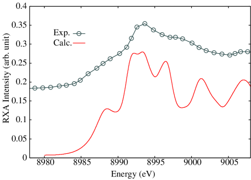
Figure 3: (Color online) Circles connected by a line represent the experimental RXA spectrum read from Ref. References, and the solid curve represents the calculated result.

Here we define the angles characterizing the scattering geometry as shown in Fig. 4. We take the following parameters for numerical calculations: $\psi=0$ rad (i.e., incident photons are in $\pi$-polarization), $\theta=\theta^{\prime}=0.24\pi$ rad, $\phi=\phi^{\prime}=0$ rad. The incident photon energy is fixed to $\omega=8994$ eV, as in the experiment [6].

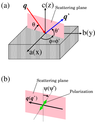
Figure 4: (Color online) Definitions of angles characterizing the scattering geometry. $\mib{q}$ and $\mib{q}$’ are the momentum vectors of the incident and emitted photons. $\theta$, $\phi$ and $\psi$ ($\theta$’, $\phi$’ and $\psi$’) are the Bragg, azimuthal and polarization angles, respectively, for incident (emitted) photons. The $a$- and $c$-axes are parallel along those of the crystalline lattice. The polarization angle is measured with respect to the scattering plane, i.e., $\psi=0$ ($\psi=\pi/2$) means that the polarization direction is parallel (perpendicular) to the scattering plane.

Typical calculated results of the total RIXS intensity $W(q,q^{\prime})$ are compared with typical experimental data in Fig. 5. Roughly speaking, there are two characteristic features: low-energy feature around 1-2 eV and high-energy feature above 5 eV. It becomes clear below that the low-energy feature originates from the $d$-$d$ excitations among the Cu-$d$ orbitals, supporting the interpretation in Ref. References. On the other hand, the high-energy feature is mainly attributed to the charge-transfer excitations between Cu-$d$ and F-$p$ states, as understood from the electronic structure in Fig. 9. Both of the features show notable polarization dependence. Particularly, the ratio of the peak intensity around 0.9 eV and 1.4 eV is drastically changed, as the polarization direction of emitted photons is changed from $\pi$’ ($\psi^{\prime}=0$) to $\sigma$’ ($\psi^{\prime}=\pi/2$), as seen in Fig. 5 (b). This behavior is qualitatively consistent with experimental data in Ref. References.

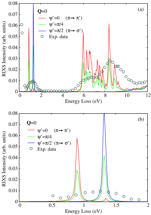
Figure 5: (Color online) Polarization dependence of calculated RIXS spectra and comparison with typical experimental data. Solid circles are the experimental data read from Ref. References (not polarization-resolved). Momentum transfer of the photon is set to the $\Gamma$ point: $\mib{Q}=\mib{q}-\mib{q}^{\prime}=0$. In (b), the low-energy region is enlarged.

Momentum dependence of calculated RIXS spectra is shown in Fig. 6. For both the cases of $\pi^{\prime}$- and $\sigma^{\prime}$- polarizations, RIXS spectra do not exhibit notable momentum dependence all over the region of energy loss. This suggests that the excitations related to these RIXS weights are spatially localized. This is in strong contrast to the cases of copper oxides, where RIXS weights show strong characteristic momentum dependence [2, 3, 4].

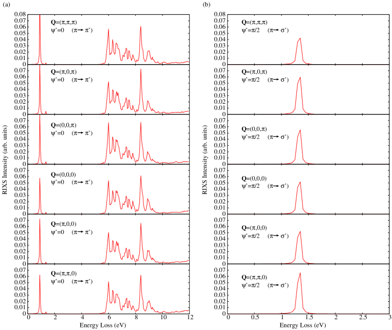
Figure 6: (Color online) Momentum dependence of the calculated RIXS spectra for two cases of polarization: (a) $\pi\rightarrow\pi^{\prime}$ ($\psi=0$, $\psi^{\prime}=0$), (b) $\pi\rightarrow\sigma^{\prime}$ ($\psi=0$, $\psi^{\prime}=\pi/2$). In (b), only the low-energy weights are shown, because the high-energy weights are almost suppressed in that scattering geometry.

The absence of notable momentum dependence in KCuF₃ is reasonably understood, since the relevant bands are rather flat, i.e., do not strongly depend on momentum, as shown in Fig. 9(a).

To elucidate the microscopic origin of each RIXS weight, we present numerical results for the process-resolved spectra defined in the last section. Calculated results of $W^{(0)}(q,q^{\prime})$ (0th-order), $W^{(s)}(q,q^{\prime})$ ($s$-process) and $W^{(p)}(q,q^{\prime})$ ($p$-process) are presented in Fig. 7.

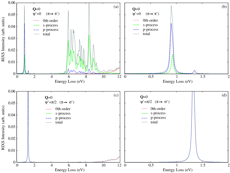
Figure 7: (Color online) Process-resolved RIXS weights for two cases of polarization. The low-energy region of each left-hand panel is enlarged in the corresponding right-hand panel. Momentum transfer of the photon is set to $\mib{Q}=\mib{q}-\mib{q}^{\prime}=0$. In (c), the 0th-order and total spectra give an almost identical curve above 8 eV. In (c) and (d), the $p$-process and total spectra give an almost identical curve below 2 eV.

From Fig. 7(a) and (b), we can see that the low-energy features around 0.9 eV and 1.4 eV are attributed to the $s$-process and $p$-process, while the high-energy charge-transfer weight originates mainly from the $s$-process. The tendency to increase above 10 eV is attributed to the 0th-order $W^{(0)}(q,q^{\prime})$, and therefore is considered as the tail of the fluorescence yield. Concerning the low-energy features, the peak feature around 0.9 eV is induced through both the $s$-process and $p$-process, while the peak feature around 1.4 eV is induced only through the $p$-process, as seen from Fig.  7.

To inspect RIXS weights more microscopically, we proceed to the calculated results of orbital-resolved spectra. Calculated orbital-resolved RIXS spectra $W_{\ell\rightarrow\ell^{\prime}}^{(s,p)}(q,q^{\prime})$ are presented in Fig. 8, where all the contributions from possible 128 orbital-excitation processes (from 8 orbitals to 8 orbitals at each of two Cu sites in the unit cell) are plotted.

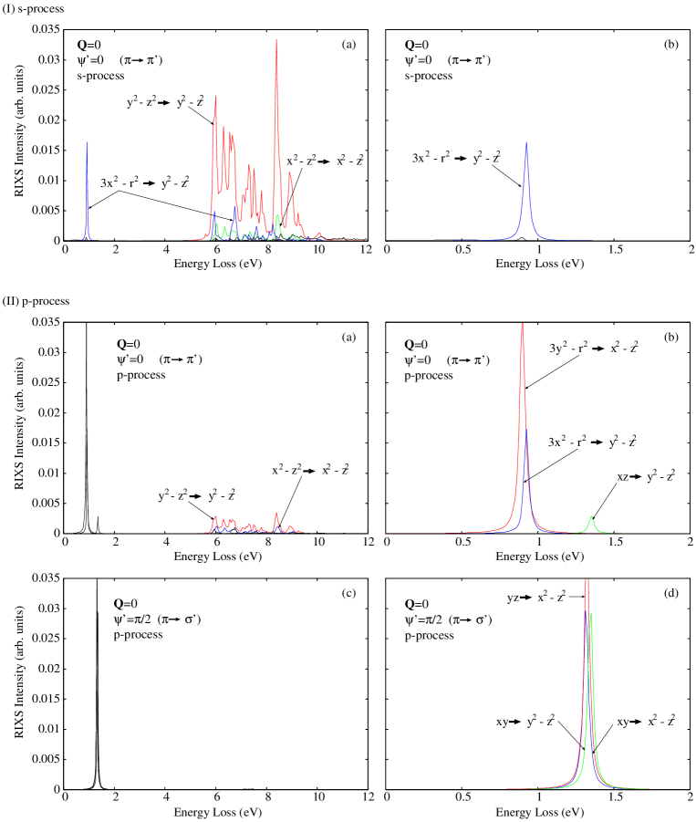
Figure 8: (Color online) Orbital-resolved RIXS weights. (I)-(a) and (b) Orbital-resolved weights in the $s$-process, $W_{\ell\rightarrow\ell^{\prime}}^{(s)}(q,q^{\prime})$. (II)-(a)-(d) Orbital resolved weights in the $p$-process, $W_{\ell\rightarrow\ell^{\prime}}^{(p)}(q,q^{\prime})$. The low-energy region of each left-hand panel is enlarged in the corresponding right-hand panel. In the $s$-process (I), the results for $\pi\rightarrow\sigma^{\prime}$ are not displayed, because the weights are almost suppressed to a negligible magnitude. Momentum transfer of the photon is set to $\mib{Q}=\mib{q}-\mib{q}^{\prime}=0$.

In the $s$-process, relevant excitations occur only among the $d\gamma$ ($e_{g}$) orbitals, as seen in Fig. 8 (I). It is remarkable that the aspect of orbital excitations is very different between the low-energy and high-energy regions: off-diagonal orbital excitations ($W_{\ell\rightarrow\ell^{\prime}}^{(s)}$ with $\ell\neq\ell^{\prime}$) are dominant in the low-energy region, while only diagonal orbital excitations ($W_{\ell\rightarrow\ell}^{(s)}$) are dominant in the high-energy region. This property also holds for the $p$-process, as seen in Fig. 8 (II). Focusing on the low-energy region (see the right-hand side of Fig. 8), we see that the RIXS weight around 0.9 eV is attributed to the orbital excitations among the $d\gamma$ ($e_{g}$) orbitals, and that around 1.4 eV is attributed to the orbital excitations from the $d\varepsilon$ ($t_{2g}$) orbitals to the $d\gamma$ ($e_{g}$) orbitals. This result is consistent with the previous simple phenomenological assignment based on symmetry properties [6].

4 Discussions

In this section, we present some remarks on the formulation and calculated results.

To explain the polarization dependence of RIXS spectra, we have included the $p$-process as well as the $s$-process. It should be noted that without the $p$-process, we could not explain the experimental spectra at the scattering geometry $\pi\rightarrow\sigma^{\prime}$: the contributions through the $s$-process to the low-energy weights around 1-2 eV are almost completely suppressed at $\pi\rightarrow\sigma^{\prime}$, as seen in Fig 7(d), which is inconsistent with the experiment. Thus it is suggested that the $p$-process essentially occurs in RIXS of KCuF₃. In the $p$-process, the Coulomb interaction $F_{pd}$ between the $p$ and $d$ orbitals at Cu sites plays an essential role. To our knowledge, the effect of $F_{pd}$ on the polarization dependence was discussed theoretically for the first time by Ishihara in the case of copper oxides [35]. It may be considered that our present work is a practical application of their mechanism to a more realistic and complex electronic structure.

To study orbital-excitation processes microscopically in detail, we have introduced orbital-resolved spectra. Such analysis has already been applied to RIXS at the Fe $K$ edge in iron-pnictide superconductors [7]. In iron pnictides, diagonal orbital excitations are dominant, and off-diagonal ones are almost irrelevant. In this sense, the orbital excitations in KCuF₃ are substantially different from those in iron pnictides. Roughly speaking, this may be because the symmetry of atom configuration around transition-metal sites is lower in KCuF₃ than in iron pnictides.

Our orbital-resolving analysis suggests that the low-energy features around 1-2 eV originate from the $d$-$d$ excitations among the Cu-$d$ orbitals. These weights do not show any notable momentum dependence as shown in Fig. 6 and Ref. References. Therefore, we should not regard them as a manifestation of orbital waves (or the so-called ‘orbitons’). Orbital waves should show some dispersive behavior as usual collective modes, if they were indeed observed.

One might consider that the calculated spectra are much sharp and show fine structures, which were not observed experimentally. Sharpness of the calculated spectra depends on the electron-hole damping rate ($\Gamma_{eh}=20$ meV in the present work). If we take a larger damping rate, then those sharp and fine structures could be smeared to be broad peaks and possibly become similar to the experimental data. However, such fine structures as obtained in our present calculation could become observable in future experiments if the resolution is improved.

In the HF calculation, we have modified one-particle energy levels by subtraction (see Appendix). Without this subtraction, we can still obtain almost the same charge-transfer weights above 5 eV, but no longer obtain the low-energy weights around 1-2 eV. They disappear to the negative side on the energy-loss axis. At present, we consider that the LDA band structure calculation, the tight-binding fitting or the HF approximation may not be sufficiently precise to evaluate the one-particle energy levels, because the one-particle energy levels are possibly much more influenced by on-site electron correlations than the hoppings between different sites are. Thus, we consider that precise evaluation of the one-particle energy levels is still difficult, while the hoppings are precisely evaluated.

5 Conclusions

We have microscopically discussed RIXS at the Cu $K$ edge in a typical orbital-ordered compound KCuF₃. In our previous works [9, 10], we have taken account of only the ‘$s$-process’, where the $1s$ core hole created in the intermediate state is screened by the Cu-$d$ electrons. However, the previous theoretical framework is insufficient to explain the experimental results, particularly, the polarization dependence in KCuF₃. We have shown that to explain the polarization dependence, the ‘$p$-process’ plays an essential role, where the $4p$ electron excited in the intermediate state is screened by the Cu-$d$ electrons, in other words, the $4p$ electron scatters the Cu-$d$ electrons in the $p$-channel.

To analyze further the RIXS process microscopically, we have introduced a new method of orbital-resolving analysis. This method enables us to clarify which orbital excitation is responsible for each spectral weight. As a result of our microscopic orbital-resolving analysis, high-energy spectral weights (above 5 eV) originate from charge-transfer excitations related to the Cu-$d\gamma$ orbitals, while the low-energy weights (below 2 eV) originate from the $d$-$d$ orbital excitations among the five Cu-$d$ orbitals. Thus we have succeeded in assigning specifically the RIXS weights to microscopic orbital-excitation processes. Our calculation supports and further goes beyond the previous phenomenological discussion.

Appendix A Hartree-Fock Approximation

Fitting to the first-principles electronic structure of the paramagnetic state, one-particle energy levels are determined for the Cu-$d$ orbitals as: $\varepsilon_{xy}=-1.84$ eV, $\varepsilon_{xz}=-2.10$ eV, $\varepsilon_{yz}=-1.78$ eV, $\varepsilon_{x^{2}-z^{2}}=-1.62$ eV, $\varepsilon_{3y^{2}-r^{2}}=-1.41$ eV at A sites, and $\varepsilon_{xy}=-1.84$ eV, $\varepsilon_{yz}=-2.10$ eV, $\varepsilon_{xz}=-1.78$ eV, $\varepsilon_{y^{2}-z^{2}}=-1.62$ eV, $\varepsilon_{3x^{2}-r^{2}}=-1.41$ eV at B sites, with respect to the Fermi level. Here we consider that these values do not reflect a realistic level scheme of the local Cu-$d$ orbitals, when we perform the HF calculation below. Therefore, we modify the one-particle energy levels of the Cu-$d$ orbitals: we subtract 2.9 eV from $\varepsilon_{\ell}$ for $d\varepsilon$ orbitals and 2.6 eV for $d_{3x^{2}-r^{2}}$ and $d_{3y^{2}-r^{2}}$ orbitals. The orbitals whose one-particle energy is here subtracted from should be almost completely filled with electrons, as well known from previous studies [20, 23, 24, 36]. This modification allows us to reproduce the electronic structure consistent with the observed magnetic ground state within the below HF calculation. Hereafter, we redefine $\varepsilon_{\ell}$ by the subtracted one-particle energy.

To describe the antiferromagnetic ground state as shown in Fig. 1, we apply the HF approximation to the tight-binding Hamiltonian $H_{n.f.}$. For the Coulomb integrals $I_{\ell_{1}\ell_{2};\ell_{3}\ell_{4}}$, we introduce the following notation:

$$J_{\ell\ell^{\prime}} \equiv I_{\ell\ell^{\prime};\ell^{\prime}\ell}$$ (26)

$$K_{\ell\ell^{\prime}} \equiv I_{\ell\ell^{\prime};\ell\ell^{\prime}}.$$ (27)

$J_{\ell\ell^{\prime}}$ and $K_{\ell\ell^{\prime}}$ are the so-called direct and exchange integrals, respectively. We assume spin polarization is induced only in the $d$ orbitals at Cu site, and take mean fields only for the Cu-$d$ electrons. The mean-field Hamiltonian for $H_{n.f.}$ is

$$H_{n.f.}^{MF} = \sum_{ii^{\prime}}\sum_{\ell\ell^{\prime}}\sum_{\sigma}t_{\ell\ell^{\prime}}({\mib r}_{i}-\mib{r}_{i^{\prime}})a_{i\ell\sigma}^{{\dagger}}a_{i^{\prime}\ell^{\prime}\sigma}+\sum_{i}^{{\rm t.m.}}\sum_{\ell}^{@\mib{r}_{i}}\biggl{[}\frac{J_{\ell\ell}}{2}\langle n_{i\ell}\rangle+\sum_{\ell^{\prime}(\neq\ell)}^{@\mib{r}_{i}}\biggl{(}J_{\ell\ell^{\prime}}-\frac{K_{\ell\ell^{\prime}}}{2}\biggr{)}\langle n_{i\ell^{\prime}}\rangle\biggr{]}n_{i\ell}$$ (28)

$$-\sum_{i}^{{\rm t.m.}}\sum_{\ell}^{@\mib{r}_{i}}\biggl{[}\frac{J_{\ell\ell}}{2}\langle\mib{m}_{i\ell}\rangle+\sum_{\ell^{\prime}(\neq\ell)}^{@\mib{r}_{i}}\frac{K_{\ell\ell^{\prime}}}{2}\langle\mib{m}_{i\ell^{\prime}}\rangle\biggr{]}\cdot\mib{m}_{i\ell}-\sum_{i}^{{\rm t.m.}}\sum_{\ell}^{@\mib{r}_{i}}\frac{J_{\ell\ell}}{4}\biggl{(}\langle n_{i\ell}\rangle^{2}-|\langle\mib{m}_{i\ell}\rangle|^{2}\biggr{)}$$

$$-\sum_{i}^{{\rm t.m.}}\sum_{\ell\neq\ell^{\prime}}^{@\mib{r}_{i}}\frac{J_{\ell\ell^{\prime}}}{2}\langle n_{i\ell}\rangle\langle n_{i\ell^{\prime}}\rangle+\sum_{i}^{{\rm t.m.}}\sum_{\ell\neq\ell^{\prime}}^{@\mib{r}_{i}}\frac{K_{\ell\ell^{\prime}}}{4}\biggl{(}\langle n_{i\ell}\rangle\langle n_{i\ell^{\prime}}\rangle+\langle\mib{m}_{i\ell}\rangle\cdot\langle\mib{m}_{i\ell^{\prime}}\rangle\biggr{)},$$

where

$$n_{i\ell} = \sum_{\sigma}d_{i\ell\sigma}^{{\dagger}}d_{i\ell\sigma}$$ (29)

$$\mib{m}_{i\ell} = \sum_{\sigma\sigma^{\prime}}d_{i\ell\sigma}^{{\dagger}}\mib{\sigma}_{\sigma\sigma^{\prime}}d_{i\ell\sigma^{\prime}},$$ (30)

using the Pauli matrix vector $\mib{\sigma}$. Within the HF theory, we should consider that the one-particle energy $\varepsilon_{\ell}$ is already including the following energy shift from the bare one,

$$\Delta^{HF}_{\ell}\equiv\frac{J_{\ell\ell}}{2}\langle n_{i\ell}\rangle+\sum_{\ell^{\prime}(\neq\ell)}^{@\mib{r}_{i}}\biggl{(}J_{\ell\ell^{\prime}}-\frac{K_{\ell\ell^{\prime}}}{2}\biggr{)}\langle n_{i\ell^{\prime}}\rangle,$$ (31)

due to the electron-electron Coulomb interaction at transition-metal site $\mib{r}_{i}$. Therefore, before determining the magnetic ground state, we need evaluate the bare one-particle energy by $\varepsilon_{\ell}^{(0)}\equiv\varepsilon_{\ell}-\Delta^{HF}_{\ell}$, where $\Delta^{HF}_{\ell}$ is evaluated from the expectation values of particle numbers $\langle n_{i\ell}\rangle$’s in the paramagnetic state using eq. (31). For the Coulomb integrals given in § 2, the obtained values of $\varepsilon_{\ell}^{(0)}$ are as follows: $\varepsilon_{xy}^{(0)}=-86.5$ eV, $\varepsilon_{xz}^{(0)}=-86.1$ eV, $\varepsilon_{yz}^{(0)}=-86.5$ eV, $\varepsilon_{x^{2}-z^{2}}^{(0)}=-85.7$ eV, $\varepsilon_{3y^{2}-r^{2}}^{(0)}=-86.2$ eV at A sites, and $\varepsilon_{xy}^{(0)}=-86.5$ eV, $\varepsilon_{yz}^{(0)}=-86.1$ eV, $\varepsilon_{xz}^{(0)}=-86.5$ eV, $\varepsilon_{y^{2}-z^{2}}^{(0)}=-85.7$ eV, $\varepsilon_{3x^{2}-r^{2}}^{(0)}=-86.2$ eV at B sites, with respect to the Fermi level. We consider that these values of $\varepsilon_{\ell}^{(0)}$ may reflect a realistic level scheme of the local Cu-$d$ orbitals: $\varepsilon_{x^{2}-z^{2}}$ and $\varepsilon_{y^{2}-z^{2}}$ are the highest level among the five local Cu-$d$ levels, as several studies suggest [36]. Maintaining these values of $\varepsilon_{\ell}^{(0)}$, we determine the mean-fields $\langle n_{i\ell}\rangle$ and $\langle\mib{m}_{i\ell}\rangle$ self-consistently. As a result, we obtain 104 diagonalized energy bands ($E_{j}(\mib{k})$, $1\leq j\leq 104$) for the antiferromagnetic ground state. The Cu-$d_{x^{2}-z^{2}}$ and Cu-$d_{y^{2}-z^{2}}$ orbitals are nearly half-filled, while the other Cu-$d$ orbitals are almost fully filled. Figure 9 shows the obtained electronic structure and the density of states for the orbital-ordered antiferromagnetic ground state. Flat bands around 5 eV and $-7$ eV with respect to the Fermi energy correspond to the upper and lower Hubbard bands, respectively. In the region between the upper and lower Hubbard bands, Cu-$d$ electronic states hybridize with F-$p$ states. Therefore our electronic structure suggests that KCuF₃ lies in the charge-transfer regime, rather than in the Mott-Hubbard regime. The bands between the upper and lower Hubbard bands seem rather flat, compared with the cases of copper oxides [9, 10], and this is a reason why the RIXS spectra do not show notable momentum dependence in KCuF₃.

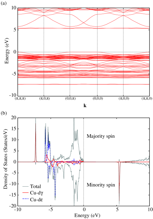
Figure 9: (Color online) (a) Band structure for the antiferromagnetic ground state calculated within the Hartree-Fock approximation. (b) Calculated density of states. Thin solid, thick solid and dashed lines represent the total density of states, the partial density of states of the Cu-$d\gamma$ and Cu-$d\varepsilon$ orbitals, respectively.

References

[1]
For a recent review, L.J.P. Ament, M. van Veenendaal, T.P. Devereaux, J.P. Hill
and J. van den Brink, Rev. Mod. Phys. 83, 705 (2011).
[2]
M.Z. Hasan, E.D. Isaacs, Z.X. Shen, L.L. Miller,
K. Tsutsui, T. Tohyama and S. Maekawa,
Science 288, 1811 (2000).
[3]
Y.J. Kim, J. P. Hill, C.A. Burns, S. Wakimoto, R.J. Birgeneau,
D. Casa, T. Gog and C.T. Venkataraman,
Phys. Rev. Lett. 89, 177003 (2002).
[4]
K. Ishii, K. Tsutsui, Y. Endoh, T. Tohyama, S. Maekawa, M. Hoesch, K. Kuzushita,
M. Tsubota, T. Inami, J. Mizuki, Y. Murakami and K. Yamada,
Phys. Rev. Lett. 94, 207003 (2005).
[5]
S. Suga, S. Imada, A. Higashiya, A. Shigemto, S. Kasai, M. Sing, H. Fujiwara,
A. Sekiyama, A. Yamasaki, C. Kim, T. Nomura, J. Igarashi, M. Yabashi and T. Ishikawa,
Phys. Rev. B 72, 081101(R) (2005).
[6]
K. Ishii, S. Ishihara, Y. Murakami, K. Ikeuchi, K. Kuzushita, T. Inami, K. Ohkawa, M. Yoshida,
I. Jarrige, N. Tatami, S. Niioka, D. Bizen, Y. Ando, J. Mizuki, S. Maekawa and Y. Endoh,
Phys. Rev. B 83, 241101(R) (2011).
[7]
I. Jarrige, T. Nomura, K. Ishii, H. Gretarsson, Y.J. Kim, J. Kim, M. Upton, D. Casa, T. Gog,
M. Ishikado, T. Fukuda, M. Yoshida, J.P. Hill, X. Liu, N. Hiraoka, K.D. Tsuei and S. Shamoto,
Phys. Rev. B 86, 115104 (2012).
[8]
K. Tsutsui, T. Tohyama and S. Maekawa,
Phys. Rev. Lett. 83, 3705 (1999); ibid. 91, 117001 (2003).
[9]
T. Nomura and J. Igarashi,
J. Phys. Soc. Jpn. 73, 1677 (2004).
[10]
T. Nomura and J. Igarashi,
Phys. Rev. B 71, 035110 (2005).
[11]
N. Pakhira, J.K. Freericks and A.M. Shvaika,
Phys. Rev. B 86, 125103 (2012).
[12]
T. Ide and A. Kotani, J. Phys. Soc. Jpn. 68, 3100 (1999);
ibid. 69, 3107 (2000).
[13]
J. van den Brink and M. van Veenendaal,
Europhys. Lett. 73, 121 (2006).
[14]
J. Igarashi, M. Takahashi and T. Nomura,
Phys. Rev. B 74, 245122 (2006).
[15]
M. Takahashi, J. Igarashi and T. Nomura,
Phys. Rev. B 75, 235113 (2007).
[16]
T. Semba, M. Takahashi and J. Igarashi,
Phys. Rev. B 78, 155111 (2008).
[17]
T. Nomura and E. Kaneshita,
J. Phys. Soc. Jpn. 81, 024707 (2012).
[18]
Y.J. Kim, J. P. Hill, S. Wakimoto, R.J. Birgeneau, F.C. Chou,
N. Motoyama, K.M. Kojima, S. Uchida, D. Casa and T. Gog,
Phys. Rev. B 76, 155116 (2007).
[19]
P. Blaha, K. Schwarz, G. Madsen, D. Kvasnicka and J. Luitz,
WIEN2k (Ver. 12.1), An Augmented PlaneWave Plus Local Orbitals Program
for Calculating Crystal Properties (ISBN 3-9501031-1-2).
[20]
S. Kadota, I. Yamada and S. Yoneyama,
J. Phys. Soc. Jpn. 23, 751 (1967).
[22]
M.D. Towler, R. Dovesi and V.R. Saunders,
Phys. Rev. B 52, 10150 (1995).
[23]
A.I. Liechtenstein, V.I. Anisimov and J. Zaanen,
Phys. Rev. B 52, R5467 (1995).
[24]
E. Pavarini, E. Koch and A.I. Lichtenstein,
Phys. Rev. Lett. 101, 266405 (2008).
[25]
A. Okazaki, J. Phys. Soc. Jpn. 26, 870 (1969).
[26]
M.T. Hutchings, E.J. Samuelsen, G. Shirane and K. Hirakawa,
Phys. Rev. 188, 919 (1969).
[27]
A. Okazaki and Y. Suemune, J. Phys. Soc. Jpn. 16, 176 (1961).
[28]
A. A. Mostofi, J. R. Yates, Y.-S. Lee, I. Souza, D. Vanderbilt and N. Marzari,
wannier90: A Tool for Obtaining Maximally-Localised Wannier Functions,
Comp. Phys. Commun. 178, 685 (2008).
[29]
J. Kunes, R. Arita, P. Wissgott, A.Toschi, H. Ikeda and K. Held,
Comp. Phys. Commun. 181, 1888 (2010).
[30]
E.U. Condon and G.H. Shortley, The Theory of Atomic Spectra
(Cambridge University Press, Cambridge, 1959).
[31]
M.T. Czyzyk and G.A. Sawatzky,
Phys. Rev. B 49, 14211 (1994).
[32]
P. Nozières and E. Abrahams,
Phys. Rev. B 10, 3099 (1974).
[34]
R. Caciuffo, L. Paolasini, A. Sollier, P. Ghigna, E. Pavarini,
J. van den Brink and M. Altarelli,
Phys. Rev. B 65, 174425 (2002).
[35]
S. Ishihara and S. Ihara, J. Phys. Chem. Solids 69, 3184 (2008).
[36]
J. Deisenhofer, I. Leonov, M.V. Eremin, Ch. Kant, P. Ghigna,
F. Mayr, V.V. Iglamov, V.I. Anisimov and D. van der Marel,
Phys. Rev. Lett. 101, 157406 (2008).