Traveling waves of the regularized short pulse equation

Abstract

In the present work, we revisit the so-called regularized short pulse equation (RSPE) and, in particular, explore the traveling wave solutions of this model. We theoretically analyze and numerically evolve two sets of such solutions. First, using a fixed point iteration scheme, we numerically integrate the equation to find solitary waves. It is found that these solutions are well approximated by a truncated series of hyperbolic secants. The dependence of the soliton’s parameters (height, width, etc) to the parameters of the equation is also investigated. Second, by developing a multiple scale reduction of the RSPE to the nonlinear Schrödinger equation, we are able to construct (both standing and traveling) envelope wave breather type solutions of the former, based on the solitary wave structures of the latter. Both the regular and the breathing traveling wave solutions identified are found to be robust and should thus be amenable to observations in the form of few optical cycle pulses.

1 Introduction

Over the last decade, there has been an intense interest in the study of ultrashort pulses with a duration of a few optical cycles, due to their numerous applications in contexts including, but not limited to, nonlinear optics, attosecond physics, light-matter interactions and harmonic generation [1]. Nonlinear media present an especially interesting setting for the propagation of such pulses due to their intensity-dependent refractive index. As a result, there is a continuously expanding volume of literature attempting to model and systematically explore such pulses using a diverse array of nonlinear wave equations, including in one-dimension (1D) the modified Korteweg-de Vries (mKdV) equation [2], the sine-Gordon (sG) equation [3, 4], and combined mKdV-sG equations [5, 6, 7] (see also the recent review [8]). Relevant models have also been developed by adapting to special settings such as, e.g., near the zero dispersion frequency [9]. In the two-dimensional case, relevant generalizations utilize the generalized Kadomtsev-Petviashvilli equation [10] and explore even features such as the collapse of ultrashort spatiotemporal pulses [11].

A considerable parallel physical as well as mathematical activity has also been focused on a different class of models that was initiated by the work of Ref. [12]. There, and in the context of nonlinear fiber optics, the so-called short-pulse equation (SPE) was derived from Maxwell’s equations. Importantly, it was shown that results obtained in the framework of the SPE model compare favorably to ones pertaining to the original Maxwell’s equations [12, 13], and are more accurate than results corresponding to the nonlinear Schrödinger equation (NLS), that is traditionally used in this (nonlinear fiber optics) context. This effort spurred numerous further studies. These were in part due to the illustrated relevance of the SPE as a suitable model, e.g., in nonlinear left-handed metamaterials [14] from the physical perspective. However, numerous interesting conclusions also arose from the mathematical setting due to the complete integrability of the model, and its intimate connection to the sG equation [15, 16], the derivation of its infinite hierarchy of conservation laws [17], as well as the identification of loop solitons, breathers and numerous other (including periodic) solutions that were identified therein [14, 18, 19, 20, 21]. Such SPE models were also developed in higher-dimensional settings, cf. [22] and integrable discretizations thereof were obtained as well [23].

Recently, a number of variant SPE models have also appeared. Arguably, the most well known example of this kind is the so-called regularized short pulse equation (RSPE) originally introduced in [24], again in the nonlinear fiber optics context. In that work, the regularization was argued as arising from the next term in the expansion of the susceptibility (within Maxwell’s equations). Importantly, it was shown that while the SPE does not support traveling wave (TW) solutions (at least in the class of piecewise smooth functions with one discontinuity), the RSPE model does exhibit such solutions (under certain conditions for the coefficients of the equation), whose existence was established via Fenichel theory and a Melnikov type argument. Extending this work, in [25], the existence of certain types of multi-pulse traveling waves was also shown by means of a geometric integral condition. We should note in passing here that other more complex higher-order correction models to the SPE have been proposed recently as, e.g., in the work of [26].

In the present work, the focus is on the RSPE model, considered in the following form:

$$u_{xt}+\alpha u+(u^{3})_{xx}+\beta u_{xxxx}=0,$$ (1)

where $u(x,t)$ is the unknown field, subscripts denote partial derivatives, while $\alpha$ and $\beta$ are real parameters (here, we use a notation similar to that of Ref. [24] and keep both parameters –although one of them can be scaled out up to its sign). Our aim is to explore traveling wave solutions of Eq. (1), which we investigate through a combination of analytical and numerical techniques. In particular, we actually explore two classes of solutions. On one hand, revisiting the proposal (and proof) of [24] about the existence of traveling waves of the RSPE that cannot be present in the SPE, we identify such solutions numerically using a fixed point iteration scheme (briefly discussed in Appendix A). We also show that such solutions can be well approximated by a truncated series of hyperbolic secant functions. On the other hand, we revisit the –arguably– most robust structures featured by the SPE (without the regularization), namely the standing and traveling wave breathers. By utilizing a reduction of the RSPE in the appropriate space and time scales (i.e., through a multi-scale expansion), we are able to revert the model to the standard NLS form. By then employing the NLS standing wave solitons, we are able to reconstruct breathers of the RSPE both of the bright and dark type (the latter only exist in the case of periodic boundary conditions). Our numerical simulations suggest the structural robustness of both classes of solutions, with the traveling waves propagating undistorted (despite the addition of small random perturbations), and with standing or traveling envelope breathers staying proximal to their NLS analogs. Hence, both classes of solutions should be possible to observe in the few optical cycle setting.

Our presentation is structured as follows. In section 2, we identify and numerically characterize (as a function of the corresponding parameters) the traveling wave (without breathing) of the RSPE. In section 3, we present the reduction of the RSPE to the NLS and reconstruct the breather solution of the former from the bright solitons of the latter. Finally, in section 4, we summarize our findings and discuss a number of directions for future studies. Some technical aspects of the analysis and computations are discussed in two appendices.

2 Solitary waves of the RSPE

We consider, at first, the solutions identified rigorously through the work of [24], namely the traveling solitary waves of Eq. (1). These are identified by going to the co-traveling frame using $\xi=x-ct$ (where $c$ is the velocity), in which the RSPE becomes:

$$-cu^{\prime\prime}+\alpha u+(u^{3})^{\prime\prime}+\beta u^{\prime\prime\prime\prime}=0,$$ (2)

where primes denote derivatives with respect to $\xi$. Recall [24] that these solutions exist when:

$$\mathrm{sgn}(c)=\mathrm{sgn}(\alpha)=\mathrm{sgn}(\beta).$$ (3)

Following the procedure of Refs. [27, 28], we obtain numerically the pertinent solitary wave for $c=\alpha=\beta=1$, by means of the spectral renormalization method. The details of this computation for our case are summarized in Appendix A. In Fig. 1 we depict this solution and its evolution according to Eq. (1). The evolution was performed using a fourth order Runge-Kutta algorithm.

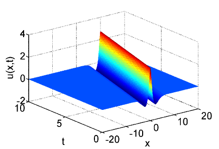
Figure 1: (Color online) The solitary wave (left) and its evolution (right) under the RSPE for $c=\alpha=\beta=1$.

To test the stability of this result we evolve again the same solitary wave but with 10% initial noise added. The resulting evolution is shown in Fig. 2. The figure is suggestive of the robustness of the solitary wave given the preservation of its traveling characteristics under the addition of noise. We note in passing that other simulations corresponding to different parameter values have led to similar results, namely indicating robustness of the traveling wave.

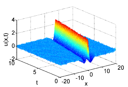
Figure 2: (Color online) The solitary wave of Fig. 1 evolved with added noise.

Next, we examine the behaviour of the solution when parameters $\beta$, $\alpha$ and $c$ change. To do this, every time a parameter changes while the other two are kept constant (equal to 1), and the solution’s characteristics values are measured i.e., we perform mono-parametric continuations. The related curves are fitted to power laws; the results are depicted in Fig. 3. The figures depict the change of the soliton’s height, width (identified as the position where the soliton crosses the $x$-axis, i.e., the location of the corresponding root), minimum and the position of the minimum. The complete fitted curves are summarized for all parameters in Table 1.

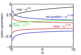
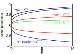
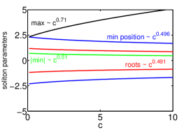
Figure 3: (Color online) The change of the soliton parameters with $\alpha$, $\beta$ and $c$.

Table 1: The change of the soliton parameters according to the RSPE parameters.

Two particular limits are of interest here: $\alpha=0$ and $\beta=0$. For the first, one can observe that the amplitude of the solution slowly grows from the mKdV limit of $\alpha=0$ (which is the starting point in our continuations), while concurrently a root emerges. In particular, the monotonic soliton of the mKdV (i.e., a ${\rm sech}$ traveling pulse) develops a shelf, which is entirely absent in the mKdV limit, and features a root which scales as a negative power of $\alpha$. This means that the region of uniform sign continuously shrinks at the center as $\alpha$ is increased. Moreover, the height of this shelf also continuously increases as a function of $\alpha$. This is consistent with the observations of Ref. [29] for the case of small values of $\alpha$. The second limit, $\beta=0$, is more complicated as there are no traveling waves for the SPE. An attempt to perturbatively explain this limit (although not for the RPSE case) was made in Ref. [30] using a variational approach since even linearization of the exact solution (of the SPE) is not tractable.

Finally, we observe a monotonic growth of the solution amplitude as $c$ is increased. On the other hand, the region associated with the central part of the solution (i.e., up to the location of the root) is very weakly affected by the variation of the speed $c$. For illustrative purposes we show in Fig. 4 the change of the solution with the speed $c$.

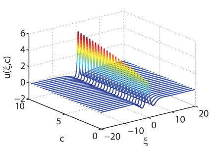
Figure 4: (Color online) The solution of the RSPE for different values of $c$.

It is also useful to develop an analytical expression for the form of the solution. In order to do so, we can approximate the traveling wave, to excellent accuracy, with a truncated series of $\mathrm{sech}$’s according to:

$$u(\xi)=a_{0}+a_{1}\mathrm{sech}(b\xi)+a_{2}\mathrm{sech}^{2}(b\xi)+a_{3}\mathrm{sech}^{3}(b\xi)+a_{4}\mathrm{sech}^{4}(b\xi)$$ (4)

The comparison between the numerically found solution and the approximation of Eq. (4) is shown in Fig. 5. The figure also presents the propagation of an initial condition in the form of Eq. (4). It is evident that the approximate solution provides a very accurate description of the dynamics, maintaining the robust traveling characteristics of the corresponding exact solution.

Figure 5: (Color online) Left: The comparison between the numerically obtained solution and the analytical approximation of Eq. (4). Right: The evolution of the approximate solution.

The exact parameters for this solution read

$$a_{0}=0.002,\;a_{1}=-6.952,\;a_{2}=23.17,\;a_{3}=-27.88,\;a_{4}=14.37,\;b=0.986,$$

while the coefficient of determination is found to be $r^{2}=0.999$.

3 Approximate envelope solitary waves of the RSPE

3.1 Multi-scale analysis and the connection to NLS

In this section we identify standing and traveling breathers of the RSPE model. Such solutions, which are reminiscent of the breather solutions of the regular SPE model (see, e.g., Refs. [14, 20, 21]), can be found by reducing the RSPE to the NLS equation by applying a formal multiscale expansion method. In particular we assume that the unknown field $u$ is a function of multiple spatial and temporal scales $(x_{0},x_{1},t_{0},t_{1},t_{2})$, defined as

$$x_{0}=x,\ \ x_{1}=\epsilon x$$

$$t_{0}=t,\ \ t_{1}=\epsilon t,\ \ t_{2}=\epsilon^{2}t,$$

where $\epsilon$ is a formal small parameter. Furthermore, we expand $u$ as:

$$u=\epsilon u_{1}+\epsilon^{2}u_{2}+\epsilon^{3}u_{3}+...$$ (5)

Then, to leading order, $O(\epsilon)$, we obtain the linear equation

$$\partial_{x_{0}}\partial_{t_{0}}u_{1}+\alpha u_{1}+\beta\partial_{x_{0}}^{4}u_{1}=0$$ (6)

whose solution is sought in the form

$$u_{1}=A(x_{1},t_{1},t_{2})e^{i\theta}+A^{*}(x_{1},t_{1},t_{2})e^{-i\theta}$$

where $\theta=kx_{0}-\omega t_{0}$ and $k\omega+\beta k^{4}+\alpha=0$ and $*$ denotes complex conjugate. The phase velocity is as usual defined as $c_{p}=\omega/k$. For $u_{2}$ to $O(\epsilon^{2})$, we have:

$$\partial_{x_{0}}\partial_{t_{0}}u_{2}+\alpha u_{2}+\beta\partial_{x_{0}}^{4}u_{2}=-[\partial_{t_{0}}\partial_{x_{1}}u_{1}+\partial_{x_{0}}\partial_{t_{1}}u_{1}+4\beta\partial_{x_{0}}^{3}\partial_{x_{1}}u_{1}]$$ (7)

Cancelling secular terms from the right hand side of Eq. (7), we obtain

$$k\partial_{t_{1}}A-(4\beta k^{3}+\omega)\partial_{x_{1}}A=0.$$ (8)

We now let $\xi=x_{1}-c_{g}t_{1}$, $t_{2}=\tau$, and $A(x_{1},t_{1},t_{2})=A(\xi,\tau)$. Then, from Eq. (8) we get the group velocity

$$c_{g}=-3k^{2}\beta+\frac{\alpha}{k^{2}}=\frac{d\omega}{dk}.$$ (9)

Additionally, Eq. (7) is now homogeneous and thus has the solution $u_{2}=0$. Finally, at $O(\epsilon^{3})$, we obtain

$$\partial_{x_{0}}\partial_{t_{0}}u_{3}+\alpha u_{3}+\beta\partial_{x_{0}}^{4}u_{3}=$$

$$-[\partial_{x_{1}}\partial_{t_{1}}u_{1}+\partial_{x_{0}}\partial_{t_{2}}u_{1}+6u_{1}(\partial_{x_{0}}u_{1})^{2}+3u_{1}^{2}\partial_{x_{0}}^{2}u_{1}+6\beta\partial_{x_{0}}^{2}\partial_{x_{1}}^{2}u_{1}].$$

Cancelation of the secular terms yields the NLS model

$$ik\partial_{t_{2}}A+\partial_{x_{1}}\partial_{t_{1}}A-6\beta k^{2}\partial_{x_{1}}^{2}A-3k^{2}|A|^{2}A=0;$$ (10)

while the third order equation reduces to

$$\quad\partial_{x_{0}}\partial_{t_{0}}u_{3}+\alpha u_{3}+\beta\partial_{x_{0}}^{4}u_{3}=-9k^{2}A^{3}e^{3i\theta}-9k^{2}{A^{*}}^{3}e^{-3i\theta}$$

with $u_{3}=Be^{3i\theta}+B^{*}e^{-3i\theta}$, where $B=\frac{-9k^{2}}{81\beta k^{4}+9\omega k+\alpha}A^{3}$.

Concluding, Eq. (10) leads in a self-consistent fashion through the above multi-scale analysis to a NLS model for the dynamics in the form of:

$$i\partial_{\tau}A+P\partial_{\xi}^{2}A+Q|A|^{2}A=0,$$ (11)

where the dispersion and nonlinearity coefficients, $P$ and $Q$, respectively, are given by:

$$P=\frac{1}{2}\frac{\partial^{2}\omega}{\partial k^{2}}=-3k\beta-\frac{\alpha}{k^{3}},\qquad Q=-3k.$$

Based on the above prescription, for given parameters $\alpha$ and $\beta$, we can select a particular wavenumber $k$, which, in turn, gives rise to a frequency $\omega$ [through Eq. (6)] and a group velocity [through Eq. (9)]. Then the exact analytical soliton solution [in the form of either a bright (for $PQ>0$) or a dark soliton (for $PQ<0$) –see below] of the NLS Eq. (11) for a given choice of $\epsilon$ can be used to reconstruct the first few orders of the solution of the RSPE, namely $u_{1}$ and $u_{3}$ (recall that $u_{2}=0$). Recombining these in our series expansion of Eq. (5), we are able to reconstruct an accurate approximation of a breather of the RSPE. A similar approximation was used in Ref. [31] in the context of mode-locked lasers.

We note in passing that it is also possible to derive a higher-order NLS (HNLS) equation, which also admits solitary wave solutions (cf. Appendix B). Nevertheless, direct numerical simulations that will be presented below show that solutions of the RSPE can already be described fairly accurately by respective soliton solutions of the regular NLS, Eq. (11), hence we restrict our numerical considerations to the latter without resorting to the HNLS below.

3.2 Bright Breathers

First, we consider moving breathers of the RSPE model, as described by the focusing NLS Eq. (11) for $PQ>0$. In this case, the NLS admits the bright soliton solution

$$A(\xi,\tau)=\sqrt{\frac{2}{|Q|}}\mathrm{sech}\left(\frac{1}{\sqrt{|P|}}\xi\right)\exp(i\tau).$$

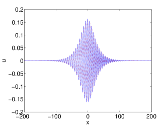
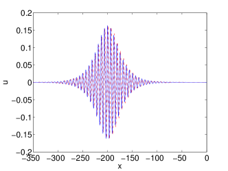
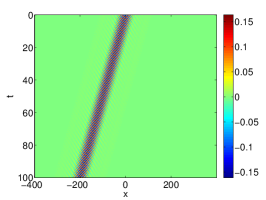
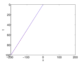
Figure 6: (Color online) Top panels: initial data as reconstructed from the NLS soliton (left), and a snapshot of the evolution at $t=100$; dashed (red) line represents the RSPE result and the solid (blue) line the NLS prediction. Bottom panels: evolution of the RSPE breather (left), its theoretical NLS analogue (middle), and center of mass evolution (right), using the same color notation as above. Here, $\epsilon=0.1$, $k=1$, $\alpha=1$, $\beta=1$, $c_{g}=-2$, $c_{p}=-2$.

The above solution can directly be compared to respective solutions derived in the framework of the RSPE. Note that, for the RSPE, the above NLS soliton represents an approximate moving breather solution. Two typical such examples, for a left moving and a right moving breather are shown in Figs. 6 and 7, respectively. The top panels show the initial data (left– common in both the “theoretical” NLS prediction and in the RSPE) and the result of the evolution at $t=100$ (top right). The agreement between the two, as illustrated by the field evolution contour plots [bottom panels, RSPE (left) and NLS (middle)], and also by the center of mass evolution (bottom right) clearly illustrates in a quantitative fashion the accuracy of the multi-scale NLS-based approximation. For these figures, the value $\epsilon=0.1$ has been used; notice, also, that in Fig. 7 refers to the case corresponding to the regular SPE limit of $\beta=0$.

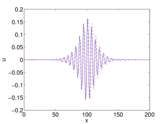
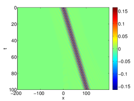
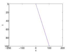
Figure 7: Same as Fig. 6, but for $\epsilon=0.1$, $k=1$, $\alpha=1$, $\beta=0$, $c_{g}=1$, $c_{p}=-1$. Notice that the choice $\beta=0$ corresponds to the SPE (rather than the RSPE) model.

A more demanding comparison is shown in Fig. 8 and also in Fig. 9 (for a finite $\beta$ of $1/3$ and a near-zero value of $\beta$, i.e., the SPE limit, respectively). In these cases, the breather is theoretically expected to be stationary. However, as observed in both figures (i.e., both in the RSPE and in the SPE case), the breather slowly drifts, over long time scales, over short distances away from its original position. Nevertheless, this drift is very slow and is nearly imperceptible over the propagation distances shown in the figure, especially so in Fig. 9.

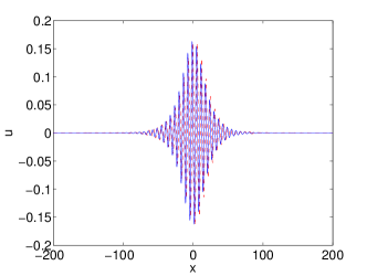
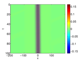
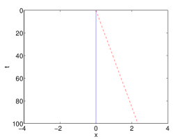
Figure 8: Same as Fig. 6 but for $\epsilon=0.1$, $k=1$, $\alpha=1$, $\beta=\frac{1}{3}$, $c_{g}=0$, $c_{p}=-\frac{4}{3}$.

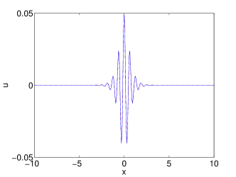
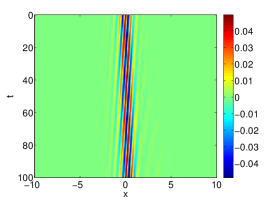
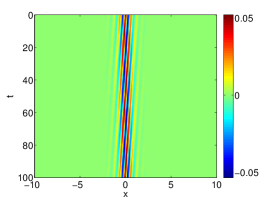
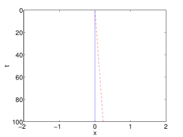
Figure 9: Same as Fig. 6 but for $\epsilon=0.1$, $k=10$, $\alpha=1$, $\beta=\frac{1}{30000}$, $c_{g}=0$, $c_{p}=-\frac{4}{300}$.

From all of the above cases, it can be readily inferred that the breather structures that were predicted to be robust in the SPE, are also found to be equally robust in the context of the RSPE in all the cases tested (including ones not shown here). Such breathers can be constructed fairly accurately, at least for sufficiently small amplitudes, using NLS bright solitons as suitable time and space modulated constituents.

3.3 Dark Breathers

The formal derivation of the NLS equation from the RSPE model allows for the prediction of still another approximate solution of the RSPE. Indeed, as mentioned in Section 3.1, the NLS model also admits dark soliton solutions, for $PQ<0$. Such a solution is of the form:

$$A(\tau,\xi)=\sqrt{|Q|}\tanh\left(\frac{\xi}{\sqrt{2|P|}}\right)\exp(-i\tau).$$

Formally, and in the framework of the RSPE, such solutions exist only for $\beta<0$ [recall that bright breathers do not exist in this case –cf. Eq. (3)]. In addition, since such solutions of the NLS exhibit nonvanishing boundary conditions at $\xi\rightarrow\pm\infty$, it is clear that they cannot be supported as approximate solutions of the RSPE on the line ($-\infty<x<+\infty$), as the only uniform stationary state of the latter is $u=0$. Nevertheless, since the field $u(x,t)$ obeying the RSPE model is real, it is possible to construct approximate dark breather solutions of the RSPE (based on the dark solitons of the NLS), using periodic boundary conditions.

Such an approximate dark breather of the RSPE is shown in Fig. 10. It is clearly observed that, once again, the NLS approximation is excellent (left and middle panels), since the coherent structure propagates undistorted over many cycles during the course of the simulation.

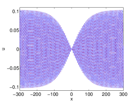
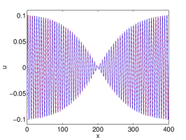
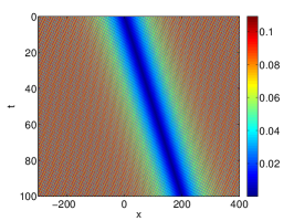
Figure 10: (Color online) The dark soliton at $t=0$ (left panel) and at $t=100$ (middle panel); again the dashed (red) line is for RSPE and solid (blue) line is for the NLS approximation. The contour plot (right panel) shows the space-time evolution of this approximate solution under the RSPE model. Here, $\epsilon=0.03$, $k=1$, $\alpha=-1$, $\beta=-1$, $c_{g}=2$, $c_{p}=2$.

4 Conclusions & Future Challenges

In the present work, we have revisited the regularized short pulse equation (RSPE) introduced in the earlier works of [24, 25]. We have examined two prototypical classes of solutions. The first one is the traveling wave (rigorously predicted to occur in a single- and multi-pulse form in [24, 25]). The second solution stems from the standard short pulse equation (SPE) without the regularization, and has the form of a breather.

For the traveling solitary waves of the equation, we used a fixed point iteration scheme to obtain these solutions for different values of the RSPE coefficients. These solutions are found in our numerical evolution simulations to be robust and maintain their characteristics even in the presence of noise. It was found that they can be well approximated by a truncated series of hyperbolic secants.

As concerns the breather solutions, they were found by means of a multi-scale expansion reducing the RSPE to the nonlinear Schrödinger (NLS) equation. From the standard sech-soliton solution of the latter, the bright breather of the RSPE was systematically reconstructed and its robustness was again shown by means of direct numerical simulations. Furthermore, using the dark (tanh-shaped) soliton solution of the NLS, we constructed approximate dark breather solutions of the RSPE model using periodic boundary conditions. These solutions, which exist for parameter values where regular (bright) breathers are not supported by the system, were found to be robust in the simulations as well.

There are many directions that one can envision in terms of possibilities for future work based on the findings of the present study. On the one hand, it would be relevant to attempt to analyze the form and stability of multi-pulse solutions both through numerical computations and through rigorous analysis (extending further the work of [25]). On the other hand, generalizing the RSPE model to higher dimensions, in the spirit of Ref. [22], would be of interest in its own right. Then, it would be relevant to explore the 2D generalization of the reductions proposed and solutions analyzed herein to examine whether such breathers, and especially genuinely 2D traveling waves, could exist in such a model. Furthermore, of particular interest may be the study of rogue waves under the RSPE and its water waves counterpart, namely the Ostrovsky equation [32]. Such studies are currently under way and will be reported in future publications.

Appendix A Spectral renormalization for the RSPE

The idea behind the spectral renormalization method is to transform the underlying equation governing the soliton into Fourier space and determine a nonlinear nonlocal integral equation coupled to an algebraic equation. This coupling generally prevents the numerical scheme from diverging. In particular, seeking traveling wave solutions of the RSPE, Eq. (1), we start our analysis by considering Eq. (2) with the boundary conditions

$$u\rightarrow 0\quad\mathrm{as}\quad|\xi|\rightarrow\infty.$$

Now define the Fourier transform (FT) pair as

$$\hat{u}(\omega) =\mathcal{F}\{u(\xi)\}=\int_{-\infty}^{\infty}u(\xi)\;e^{-i\omega\xi}\;d\xi,$$

$$u(\xi) =\mathcal{F}^{-1}\{\hat{u}(\omega)\}=\frac{1}{2\pi}\int_{-\infty}^{\infty}\hat{u}(\omega)\;e^{i\omega\xi}\;d\omega.$$

Applying the FT to Eq. (2) we obtain the equation:

$$(\alpha+c\omega^{2}+\beta\omega^{4})\hat{u}-\omega^{2}\mathcal{F}\{u^{3}\}=0.$$

In order to construct a solution so that its amplitude does not grow indefinitely nor tends to zero with each iteration, we introduce $v(\xi)$ such that:

$$u(\xi)=\lambda v(\xi)\Leftrightarrow\hat{u}(\omega)=\lambda\hat{v}(\omega),$$

where $\lambda$ is to be determined. Then $v(\xi)$ satisfies:

$$(\alpha+c\omega^{2}+\beta\omega^{4})\hat{v}-\lambda^{2}\omega^{2}\mathcal{F}\{v^{3}\}=0.$$

Multiplying by $\hat{v}^{*}(\omega)$ and integrating over the entire space $\omega$ we find the relation:

$$\int_{-\infty}^{\infty}(\alpha+c\omega^{2}+\beta\omega^{4})|\hat{v}|^{2}\;d\omega-\lambda^{2}\int_{-\infty}^{\infty}\omega^{2}\mathcal{F}\{v^{3}\}\hat{v}^{*}\;d\omega=0,$$

which must then be solved for $\lambda$, thus determining the necessary constant so that the solution will not simply decay to zero or blow-up after an iteration. Finally, the solution is obtained by iterating as follows:

$$\hat{v}_{n+1}(\omega)=\frac{\lambda_{n}^{2}\omega^{2}\mathcal{F}\{v_{n}^{3}\}}{(\alpha+c\omega^{2}+\beta\omega^{4})}.$$

Recall, that $\alpha$, $\beta$ and $c$ share the same sign so the denominator has no zeros. This iteration is for $n>0$. When $n=0$ an initial guess is required, typically a Gaussian.

To ensure that convergence is achieved we employ in our numerical codes three criteria. We demand convergence in $\lambda$, namely

$$|\lambda_{n+1}-\lambda_{n}|<\delta,$$

convergence in $v$,

$$|v_{n+1}-v_{n}|<\delta,$$

where $\delta$ is the accuracy we desire, say $10^{-9}$ or $10^{-10}$, and most importantly when these two conditions are satisfied the solution satisfies the equation up to the same accuracy $\delta$, or in other words, the residual is of that order.

Appendix B The higher-order NLS equation and its soliton solutions

The multiscale analysis presented in Sec. 3.1 leads to the regular NLS model, Eq. (11), at the order $O(\epsilon^{3})$. At the next order of approximation, namely at $O(\epsilon^{4})$, it is possible to derive a higher-order NLS, which incorporates third-order dispersion and higher-order nonlinear terms. This model is of the form,

$$i\partial_{\tau}A+P\partial_{\xi}^{2}A+Q|A|^{2}A+i\delta\partial_{\xi}^{3}A+i\mu|A|^{2}\partial_{\xi}A+i\nu A^{2}\partial_{\xi}A^{*}=0,$$ (12)

where the coefficients of the higher-order terms are given by:

$$\delta=4\beta\epsilon,\qquad\mu=12\epsilon,\qquad\nu=6\epsilon.$$

Following the analysis of Ref. [33], it is possible to derive exact travelling wave solutions of Eq. (12), in the form of solitary waves. Such solutions are sought in the form:

$$A(\xi,\tau)=\Phi(\eta)\exp[i(K\xi-\Omega\tau-\theta)],\qquad\eta=\xi-V\tau,$$

where $\Phi(\eta)$ is an unknown real function, while $K$, $\Omega$ and $V$ denote the wavenumber, angular frequency and velocity of the wave ($\theta$ is a constant phase). Introducing the above ansatz into Eq. (12), and separating real and imaginary parts, we derive the following ordinary differential equations (ODEs):

$$(P-3\delta K)\Phi^{\prime\prime}+(\Omega-PK^{2}+\delta K^{3})\Phi+[Q-(\mu+\nu)K]\Phi^{3}=0,$$ (13)

$$\delta\Phi^{\prime\prime\prime}+(-V+2PK-3\delta K^{2})\Phi^{\prime}+(\mu+\nu)\Phi^{2}\Phi^{\prime}=0,$$ (14)

where primes denote derivatives with respect to $\eta$. Observing that the compatibility condition of the above equations (which is found upon differentiating Eq. (13) once with respect to $\eta$) is

$$\frac{\Omega-PK^{2}+\delta K^{3}}{P-3\delta K}=\frac{-V+2PK-3\delta K^{2}}{\delta}=\lambda_{1},$$ (15)

$$\frac{3[Q-(\mu+\nu)K]}{P-3\delta K}=\frac{\mu+\nu}{\delta}=\lambda_{2},$$ (16)

we find that Eqs. (13), (14) are equivalent to the following ODE:

$$\Phi^{\prime\prime}+\lambda_{1}\Phi+\lambda_{2}\Phi^{3}=0.$$ (17)

Then, utilizing Eq. (17), it is straightforward to show (see, e.g., Ref. [33] for details), that there exist bright and dark solitary wave solutions of Eq. (12). In particular, in the case $\lambda_{1}<0$ and $\lambda_{2}>0$, we derive the bright solitary wave

$$\Phi(\eta)=\left(\frac{2|\lambda_{1}|}{\lambda_{2}}\right)^{1/2}{\rm sech}(\sqrt{|\lambda_{1}|}\eta),$$ (18)

while in the case $\lambda_{1}>0$ and $\lambda_{2}<0$, we derive the dark solitary wave

$$\Phi(\eta)=\left(\frac{\lambda_{1}}{|\lambda_{2}|}\right)^{1/2}\tanh\left(\sqrt{\frac{|\lambda_{2}|}{2}}\eta\right).$$ (19)

Observing that the three parameters $K$, $\Omega$ and $V$ of the above solutions are connected via two equations, (15)-(16), it is clear that the solitary waves in Eqs. (18)-(19) are characterized by one free parameter. Fixing this parameter, we can appropriately fix the sign of $\lambda_{1}$; then, taking into regard that $\lambda_{2}=(\mu+\nu)/2=(9/2)\beta$, we find that bright (dark) solitary waves for $\beta>0$ ($\beta<0$), consistently with the results obtained in the framework of the regular NLS model.

References

References

- [1] T. Brabec and F. Krausz, Rev. Mod. Phys. 72, 545 (2000).
- [2] I. V. Mel’nikov, D. Mihalache, F. Moldoveanu, and N.-C. Panoiu, Phys. Rev. A 56, 1569 (1997).
- [3] H. Leblond and F. Sanchez, Phys. Rev. A 67, 013804 (2003).
- [4] I.V. Mel’nikov, H. Leblond, F. Sanchez, and D. Mihalache, IEEE J. Sel. Top. Quantum Electron. 10, 870 (2004).
- [5] H. Leblond, S.V. Sazonov, I.V. Mel’nikov, D. Mihalache, and F. Sanchez, Phys. Rev. A 74, 063815 (2006).
- [6] H. Leblond, I.V. Mel’nikov, and D. Mihalache, Phys. Rev. A 78, 043802 (2008).
- [7] H. Leblond and D. Mihalache, Phys. Rev. A 79, 063835 (2009).
- [8] H. Leblond and D. Mihalache, Phys. Rep. 523, 61 (2013).
- [9] S. Amiranashvili, A.G. Vladimirov and U. Bandelow, Eur. Phys. J. D 58, 219 (2010).
- [10] I.V. Mel’nikov, D. Mihalache, and N.-C. Panoiu, Opt. Commun. 181, 345 (2000).
- [11] H. Leblond, D. Kremer, and D. Mihalache, Phys. Rev. A 81, 033824 (2010).
- [12] T. Schäfer and C.E. Wayne, Physica D 196, 90 (2004).
- [13] Y. Chung, C.K.R.T. Jones, T. Schäfer, and C.E. Wayne, Nonlinearity 18, 1351 (2005).
- [14] N.L. Tsitsas, T.P. Horikis, Y. Shen, P.G. Kevrekidis, N. Whitaker, and D.J. Frantzeskakis, Phys. Lett. A 374, 1384 (2010).
- [15] A. Sakovich and S. Sakovich, J. Phys. Soc. Jpn. 74, 239 (2005).
- [16] Y. Yao, Y. Huang, G. Dong and Y. Zeng, J. Phys. A: Math. Theor. 44, 065201 (2011).
- [17] J.C. Brunelli, J. Math. Phys. 46, 123507 (2005).
- [18] T.P. Horikis, J. Phys. A: Math. Theor. 42, 442004 (2009).
- [19] A. Sakovich and S. Sakovich, J. Phys. A: Math. Gen. 39, L361 (2006).
- [20] Y. Shen, F. Williams, N. Whitaker, P.G. Kevrekidis, A. Saxena, and D.J. Frantzeskakis, Phys. Lett. A 374, 2964 (2010).
- [21] Y. Matsuno in: Handbook of Solitons: Research, Technology and Applications, edited by S.P. Lang and S.H. Bedore (Nova Publishers, NY, 2009).
- [22] Y. Shen, N. Whitaker, P.G. Kevrekidis, N.L. Tsitsas and D.J. Frantzeskakis, Phys. Rev. A 86, 023841 (2012).
- [23] B.F. Feng, K. Maruno and Y. Ohta, J. Phys. A: Math. Gen. 43, 085203 (2010).
- [24] N. Constanzino, V. Manukian and C.K.R.T. Jones, SIAM J. Math. Anal. 41, 2088 (2009).
- [25] V. Manukian, N. Constanzino, C.K.R.T. Jones, B. Sandstede, J. Dyn. Diff. Eqs. 21 607 (2009).
- [26] K. Levent, Y. Chung and T. Schäfer, J. Phys. A: Math. Gen. 46, 285205 (2013).
- [27] M.J. Ablowitz and Z.H. Musslimani, Opt. Lett. 30, 2140 (2005).
- [28] M.J. Ablowitz and T.P. Horikis, Eur. Phys. J. Special Topics 173, 147 (2009).
- [29] Y. Kodama and M.J. Ablowitz, Stud. Appl. Math. 64, 225 (1981).
- [30] E.D. Farnum and J.N. Kutz, J. Opt. Soc. Am. B 30, 2191 (2013).
- [31] J.N. Kutz and E. Farnum, in Non-Diffracting Waves, eds. H.E. Hernández-Figueroa, E. Recami, M. Zamboni-Rached, p. 451, 2013.
- [32] L. Ostrovsky, Oceanology 18, 119 (1978).
- [33] K. Hizanidis, D.J. Frantzeskakis, and C. Polymilis, J. Phys. A: Math. Gen. 29, 7687 (1996).