Linglong Kong and Douglas P. Wiens111Department of Mathematical and Statistical
Sciences; University of Alberta, Edmonton, Alberta; Canada T6G 2G1. e-mail:
lkong@ualberta.ca, doug.wiens@ualberta.ca
Abstract We give methods for the construction of
designs for regression models, when the purpose of the investigation is the
estimation of the conditional quantile function and the estimation method is
quantile regression. The designs are robust against misspecified response
functions, and against unanticipated heteroscedasticity. The methods are
illustrated by example, and in a case study in which they are applied to
growth charts.
Key words and phrases Asymptotic mean squared error;
B-splines; Compound design; Exchange algorithm; Genetic algorithm; Growth
charts; Heteroscedasticity; Minimax bias; Minimax mean squared error;
Nonlinear models; Regression quantiles; Uniformity
The need for robust methods of analysis in statistical investigations was
convincingly made by Huber (1981), in whose work one finds a concentration on
robustness against departures from the investigator’s assumed parametric model
of the distribution generating the data. Box and Draper (1959) had
earlier made the case that, when there is any doubt about the form of the
response model in a regression analysis in which the choice of design
is under the control of the experimenter, then such choices should be made
robustly, i.e. with an eye to the performance of the resulting designs under
a range of plausible alternate models. A focus of the work of Box and Draper
was on designs robust against polynomial responses of degrees higher than that
anticipated by the experimenter. This was extended in one direction by Huber
(1975), who derived minimax designs for straight line fits; these
minimize the maximum mean squared error of the fitted values, with the maximum
taken over a full -neighbourhood of the experimenter’s assumed
response. This work, for which it was assumed that the regression estimates
would be obtained by least squares, has in turn been extended in numerous
directions – Li (1984) to finite design spaces, Wiens (1992) to multiple
regression, Woods, Lewis, Eccleston and Russell (2006) to GLMs, Li and Wiens
(2011) to dose-response studies, to list but a few.
A method of estimation with a degree of distributional robustness is
M-estimation (Huber 1964). Such methods convey robustness against outliers in
the response variable of a regression, but have influence functions which are
unbounded in the factor space. For random regressors this unboundedness may be
addressed by the use of Bounded Influence (BI) methods (Maronna and Yohai
1981, Simpson, Ruppert and Carroll 1992); otherwise it can be controlled by
the design. Designs to be used in league with M- or BI-estimates have been
studied by Wiens (2000) and Wiens and Wu (2010). In the latter article it was
found that there is very little difference between designs optimal (in some
sense, robust or not) for least squares and those for M-estimation; this is
however not the case for BI-estimation.
An increasingly popular method of estimation and inference was furnished by
Koenker and Bassett (1978), who elegantly restated the case for robustness,
went on to extend the notion of univariate quantiles to regression quantiles,
and derived quantile regression methods of estimating the conditional
quantile function. Koenker and Bassett point out that the influence function
of a quantile regression estimator is, like that of an M-estimator, unbounded
in the factor space. This can again be addressed by the design. Dette and
Trampisch (2012) have recently studied this problem, assuming that the
experimenter’s assumed model is correct; to date there is no published work on
designs for quantile regression methods, which extends the natural robustness
of these methods against outliers to robustness against misspecified response
models. We do so in this article, and also consider robustness against
unanticipated heteroscedasticity.
The need for optimal designs for quantile regression methods was convincingly
articulated by Dette and Trampisch (2012). That for robustness of design can
arise in numerous ways. Beyond the obvious – that in many studies the fitted
model is adopted largely as an article of faith – there are numerous
scenarios in which the final goal is to fit models which might not fall within
a standard design paradigm, but for which a preliminary study with reasonable
efficiency against a range of models might furnish a point from which to
expand the investigations. Some recent examples of this employ quantile
regression in model selection (Behl, Claeskes and Dette 2014), ecological
studies (Martínez-Silva, Roca-Pardiñas, Lustres-Pérez,
Lorenzo-Arribas and Cadaro-Suárez 2013), financial modelling (Rubia and
Sanchis-Marco 2013), and the fitting of time-varying coefficients (Ma and Wei
2012). In such cases the initial fitted model might be non-linear; we address
this in §2.2.
In §2 we outline our notion of misspecified
response models, and set the stage for the optimality problems to be addressed
in subsequent sections. The misspecification engenders a bias in the estimate,
motivating our use of mean squared error (mse) of the estimate of the
conditional quantile function as a measure of the loss. In
§3 we illustrate some designs which minimize the
maximum mse, with this maximum taken over certain very broad classes
of response misspecifications. Then in §4
we specialize to designs which address only the bias component of the
mse – this is somewhat of a return to the findings of Box and
Draper, who state (Box and Draper 1959, p. 622) that ‘… the optimal design
in typical situations in which both variance and bias occur is very nearly the
same as would be obtained if variance were ignored completely and the
experiment designed so as to minimize the bias alone.’
The bias-minimizing designs turn out to have design weights proportional to
the square roots of the variance functions, when these functions are known. If
instead they are also allowed to range over a certain broad class of variance
functions, then uniform designs minimize the maximum bias over both
types of departures from the experimenter’s assumptions. In
§5 this optimality of uniform designs is
extended to minimization of the maximum mse over both types of
departures; we find that the minimax designs are uniform on their support.
Finally, in §6, we illustrate the theory we have
developed in an application to growth charts, in which the regressors are
cubic B-splines and the appropriate choice of knots, and their locations, is
in doubt.
We have posted software (see http://www.stat.ualberta.ca/~wiens/home page/pubs/qrd.zip) which runs on matlab, and instructions
for its use, to compute the optimal designs in all of these scenarios. All
derivations and longer mathematical arguments are in the Appendix, or in the
online addendum Kong and Wiens (2014).
2 Approximate quantile regression models
To set the stage for the examples of subsequent sections, suppose that an
experimenter intends to make observations on random variables with
structure
(1)
for a -vector of functionally independent regressors, each
element of which is a function of a -vector of independent
variables chosen (the ‘design’) from a space . We assume that the errors
are i.i.d., and that the variance function is strictly positive on the support of the design.
For a fixed , is to be the conditional -quantile of , given :
(2)
(We write for the distribution function of a
random variable .)
Now suppose that (1) is only an approximation, and that in
fact
(3)
for some ‘small’ model error . The dependence of on
is necessary for a sensible asymptotic treatment – in order that bias and
variance remain of the same order we will assume that . For fixed sample sizes this is moot.
The experimenter, acting as though and is constant, computes the quantile regression estimate
(4)
where is the ‘check’ function , with
derivative .
We will consider two types of design spaces . The first is discrete,
with possible design points ; here is arbitrary. We also consider a continuous, compact
design space, with Lebesgue measure vol, in which case the design is
generated by a design measure .
Initially, we shall unify the presentation by writing sums of the form
, in
which a fraction of the observations are to be made
at the design point , as Lebesgue-Stieltjes
integrals, viz. as . We assume that the design measure has a
weak limit for which
Under (3) the meaning of becomes
ambiguous. Thus we define this ‘true’ regression parameter as that making the
experimenter’s approximation (1) most accurate, under the
experimenter’s assumption of homoscedasticity. For a discrete design space
this is
(5)
Carrying out the minimization in (5) and evaluating at
:
(6)
where is the density of . We now define
, so that
(7)
In a continuous design space the average is replaced by an integral – see
(8b).
The true conditional -quantile is predicted by , and our approach is to
obtain the asymptotic mean squared error matrix mse of the parameter estimates, thus obtaining the
average – over – mse of these predicted values, and to
maximize this average mse over the appropriate choice
(8a)
(8b)
This is carried out in §2.3. We also consider
classes of variance functions. These may be independent of the design or –
see (18) – vary with the designs weights, in which case we also
maximize the mse over this class. In any event we then go on to find
the mse-minimizing designs , using a variety of
analytic and numerical techniques.
In most cases the optimal designs must be approximated in order
to implement them in finite samples; for example when we will do this by
placing the design points at the quantiles
(9)
or at the closest available points in discrete design spaces. For the
situation is more interesting and some suggestions are in Fang and Wang (1994)
and Xu and Yuen (2011); an intriguing possibility as yet (to our knowledge)
unexplored is the use of vector quantization to approximate the designs.
2.1 Asymptotics
In (8) the imposition of (7), and its analogue in
continuous spaces, ensures the identifiability of the parameter in
(3). The bounds of force the errors due to
variation, and those due to the bias engendered by the model misspecification,
to remain of the same order asymptotically – a situation akin to the
imposition of contiguity in the asymptotic theory of hypothesis testing.
Define
(10a)
(10b)
(10c)
Assume that the support of is large enough that and are positive definite. Define the target
parameter to be the asymptotic solution to
(B.6), so that
(11)
in agreement with (B.5). The proof of the asymptotic normality of the
estimate runs along familiar lines – see Knight (1998) and Koenker (2005) –
and so we merely state the result. Complete details are in Kong and Wiens (2014).
Theorem 1
Under conditions (A1) – (A3) the quantile
regression estimate of the parameter
defined by (B.7) is asymptotically normally
distributed:
2.2 Nonlinear models
Dette and Trampisch (2012) obtained (non-robust) designs for quantile
regression and nonlinear models; these were locally optimal,
with, in our notation, (2) replaced by , where
is evaluated at fixed
values of those elements of which enter in a nonlinear
manner. Some robustness against misspecifications of these local parameters
was then introduced by considering Bayesian and maximin designs. In this
article the examples pertain only to linear models. However, since
(as also in Dette and Trampisch 2012), our approach is asymptotic in nature,
the results presented here are easily modified to accommodate nonlinear
models. The definition (B.6) of the estimate is replaced by
,
and then, in all occurrences,
is to be replaced by the gradient . With these changes Theorem
4 continues to hold, as does the rest of the
theory of the article. The robustness is then attained against
misspecifications in the functional form of , possibly but not necessarily arising from
misspecified parameters.
We now introduce a measure of the asymptotic loss when the conditional
quantile , for , is incorrectly
estimated by . For a
discrete design space this measure is the limiting average mean squared error
We now write merely for . We impose a bound for a given
, and we denote by the maximum eigenvalue of a
matrix. The maximum value of amse over is given in the
following theorem.
Theorem 2
For a discrete design space define
and
(13)
Then amse is times
(14)
where .
The first component () of
arises solely from variation,
the second () from (squared)
bias. Note that (14 ) depends on only through
and through . We
may thus without loss of generality take and parameterize the
designs solely by , which may be chosen by the
experimenter, representing his relative concern for errors due to bias rather
than to variation.
3 Examples: Designs minimizing max
MSE for fixed variance
functions
Before extending the theory presented thus far, we illustrate it for some
representative, fixed variance functions in two cases – approximate straight
line regression in a discrete design space, and approximate quadratic
regression in a continuous design space. The development of the first case is
given in some detail in the Appendix; that for the second is outlined only briefly.
3.1 Discrete design spaces
For least squares regression problems with univariate design variables and
homoscedastic variances, optimally robust designs have been constructed by,
among others, Fang and Wiens (2000), who computed exact designs by simulated
annealing. Here we construct optimal designs for heteroscedastic quantile
regression problems and also take a different approach to the implementation
– we obtain exact optimal values and then
implement the designs as at (9).
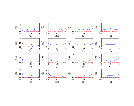
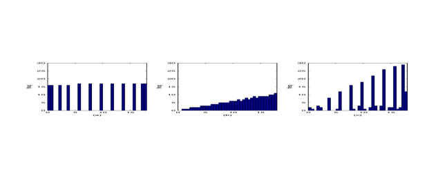
Figure 1: Minimax (over ) design measures for heteroscedastic
straight line regression, , normalized so that bar area = 1. Columns 1
– 4 use respectively; rows 1 – 4 use , ,
, respectively. The
bullets below the horizontal axes are the locations of design points,
implemented as at (9).
For a fixed variance function and a discrete design space we seek a design
minimizing (14). We illustrate the method in
the case of approximate straight line models – – and suppose that the
design space consists of points in . The
space is symmetric in that if () and denotes the
reversal then . We consider symmetric designs, i.e. designs for which
, with
, satisfies . We also assume a symmetric but arbitrary
variance function .
The designs are obtained by variational arguments followed by a constrained
numerical minimization; the details are in the Appendix. See Figure
1 for representative plots of the designs, scaled so as to have
unit area. In these plots the bullets below the horizontal axes are the
locations of design points, implemented as at (9). In the
case of homoscedasticity (plots (e) - (h)) the designs for very small
are close in nature to their non-robust counterparts, placing point masses at
. As increases these replicates spread out into clusters near
and, depending upon the variance function, possibly near as well.
The limiting behaviour as is studied in
§4.
3.2 Continuous design spaces
The continuous case requires special consideration. Rather than amse
at (12) we use instead the integrated mean squared error
together with , and obtain
In order that the maximum imse be finite, it is necessary that the
design measure be absolutely continuous. That this should be so is intuitively
clear – if in (B.8) places positive mass on sets of
Lebesgue measure zero, such as individual points, then may be
chosen arbitrarily large on such sets without altering its membership in
, and one can do this in such a way as to drive imse beyond all bounds, through (B.8a). A formal proof may be based on
that of Lemma 1 in Heo, Schmuland and Wiens (2001).
When implementing continuous designs we discretize; for instance when there is
only one covariate we employ (9). As a referee has pointed out,
this might result in an unbounded imse along particularly
pathological sequences . A possible
alternative, which we do not illustrate here since it is unlikely to find
favour with practitioners, is to randomly choose design points from the
optimal design measure; in the parlance of game theory this would thwart the
intentions of a malevolent Nature, which can then not anticipate the design.
In the same vein Bischoff (2010) states a criticism, in a context of
discretized, absolutely continuous, lack-of-fit designs as proposed by Wiens
(1991) and Biedermann and Dette (2001), of the very rich class of
alternatives, analogous to (8b), used by those authors.
Bischoff suggests using a smaller class of alternatives; here we are however
in accord with Wiens (1992), who states ‘Our attitude is that an
approximation to a design which is robust against more realistic alternatives
is preferable to an exact solution in a neighbourhood which is unrealistically
sparse.’
We write for the density of when
dealing with continuous design spaces and take (, as in the
discrete case).
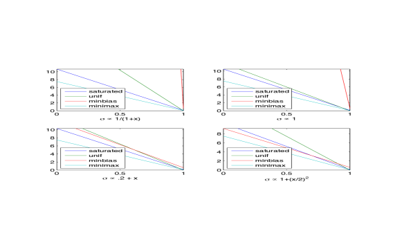
Theorem 3
For a continuous design space define
and as at (13), with
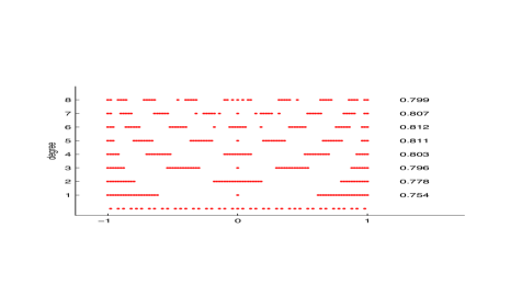
Figure 2: Minimax (over ) design densities for heteroscedastic
quadratic regression on . Columns 1 – 4 use
respectively; rows 1 – 4 use , , , respectively. The bullets on the
horizontal axes are the locations of design points, implemented as at
(9).
As an example we minimize imse for approximate quadratic regression,
i.e. , and a fixed variance function
, over the design space . Similar
problems, assuming homoscedasticity, were studied previously by Shi, Ye and
Zhou (2003) using methods of nonsmooth optimization, and by Daemi and Wiens
(2013) following the methods used here and outlined in the Appendix.
We show in the Appendix that the minimizing density is of the form
(15)
for polynomials ,
. The ten constants forming are chosen to
minimize the loss at
(14) over , subject to . Some examples are illustrated in Figure 2.
Again there is a pronounced increase in the spreading out of the mass as
increases, and again under homoscedasticity these masses are initially
concentrated near and , as in the non-robust case. It is rather
evident from the plots in the rightmost panels of Figure 2 that,
as , the density becomes proportional to
, a phenomenon explained in the following section.
4 Bias minimizing designs
The following result is quite elementary, but since we use it repeatedly we
give it a formal statement and proof.
Proposition 1
(i) Suppose that is discrete, that the function
is defined on and
that exists for ,
and (),
and is invertible for and . Then, under the ordering
‘’ with respect to positive semidefiniteness,
(16)
(ii) Suppose that is continuous, that the function is defined on and that
exists for , and , and is
invertible for and . Then (16) holds.
In discrete design spaces we define . It then follows from Proposition 1 that
; note as well that
.
Together these imply that
(17)
Motivated by the remark of Box and Draper (1959) quoted in §1 of this
article we note that, if the experimenter seeks robustness only against errors
due to bias (so that ), whether arising from a misspecified response
model or a particular variance function ,
then the maximum bias is minimized by , since then and the
lower bound in (17) is attained.
Similarly, in a continuous design space the maximum bias is minimized by
; for this we use
, in place of
and obtain a lower bound of in
(17).
If the form of the variance function is in doubt, then a minimax approach
dictates taking a further maximum over a class of such functions. We consider
the class of variance functions given by
(18)
is the required constant of proportionality determined by, e.g.,
. In the
discrete case define
Note that . If then ,
which by Proposition 1 exceeds ; this in turn is minimized by the uniform
design , with . Thus this approximate
design, which we implement as at (9), is minimax with respect to
bias, over . Similarly, in a continuous design space the minimax
bias design is the continuous uniform: vol.
This discussion has revealed why the minimax designs exhibited in Figures
1 and 2 become proportional to as , and for are uniform if the
maximization is also carried out over . For , if the form
of is known then this knowledge can be used to
increase the efficiency of the design, relative to uniformity. In the next
section we show that, if is unknown but is
allowed to range over , then uniform (on their support) designs
are again minimax with respect to mse.
Several cases are of interest for fixed . The case corresponds to
homoscedasticity. That for is treated in Kong and Wiens (2014). If
(a case which turns out to be least favourable – see the proof of Lemma
1), then
In this case the optimal, approximate design is again uniform on
all of : . And again in the parlance of game
theory, the experimenter’s optimal reply to Nature’s strategy of placing the
variances proportional to the design weights is to design in such a way that
this variance structure is in fact homoscedastic.
To see that is uniform, note that at this design we have
and
, so that
, and it
suffices to note that for any other design , by Proposition
1, .
Similarly, in the continuous case the uniform design, with density , minimizes .
To extend these optimality properties of uniform designs to all of , we first consider the discrete case, and define . By the
following lemma, a minimax design is necessarily uniform on its support.
Lemma 1
If is a design with -point support
(), placing mass at , and
is the design placing mass at each point , then and
By Lemma 1 the search for minimax designs reduces to
searching for support points on which the design is to be uniform. Since
increases, in the sense of positive semidefiniteness,
as increases, a minimax design necessarily has maximum
support size. Among approximate designs the optimal choice is thus . Among exact designs must have
support size ; the support points are those
minimizing
(19)
with . We are then seeking a compound optimal design, for which problems
some general theory has been furnished by Cook and Wong (1994); in our case
there is however the additional restriction to uniformity.
Figure 3: Minimax compound, uniform designs minimizing amse for polynomial regression of degrees
; , , . Bullets indicate design points; bottom
line is the -point implementation of the design .
Efficiencies are given at the right.
Example 5.1. In the case of straight line models and
symmetric designs on a symmetric interval, . Both components of are decreased by progressively including in the support the largest
remaining design points, so as to ‘increase’ . If
is odd then must be in the support; the remaining points – all points
if is even – are the symmetrically placed design points of largest absolute value.
If is a multiple of , say , then this design is replicated
times. If for then an exact uniform design is not attainable
if . A possible implementation is to place observations at each of
the points in the design space, and to append to this the symmetrically placed design points of largest absolute value
(and , if is odd).
Example 5.2. We have found an exchange algorithm to be very
effective at constructing compound designs minimizing (19). This
has been carried out for polynomial regression over ,
with the restriction to symmetric designs. See Figure 3, in
which some typical cases are displayed and compared with the approximate
design , implemented as at (9). The
efficiencies given in the figure have been found to be quite stable over other
choices of and .
In a completely analogous manner we find that the continuous uniform design,
with density , minimizes the maximum
of over and .
6 Case study: Robust design in growth charts
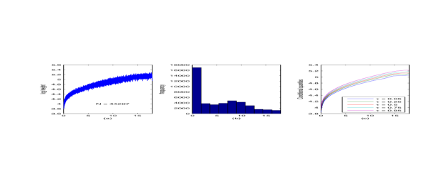
Figure 4: (a) vs. age in full dataset;
(b) frequencies of ages; (c) conditional quantile curves computed from full
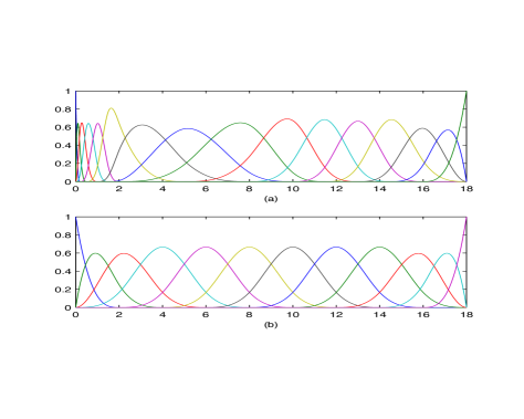
dataset.Figure 5: Cubic splines for growth study. (a) ‘Full’ spline basis is of
dimension 16; (b) ‘Reduced’ basis of dimension 12 has fewer and different
internal knots.Figure 6: Designs (uniform design not shown) computed for Example 6.1: (a)
Saturated design on 12 points; (b) Minbias design; (c) Minimax design with
.Figure 7: Maximum amse
vs. for various choices of and the designs of Example 6.1; the
minimax design was tailored to .
Growth charts, also known as reference centile charts, were first conceived by
Quetelet in the century, and are commonly used to screen the
measurements from an individual subject in the context of population values;
to this end they are used by medical practitioners, and others, to monitor
people’s growth. A typical growth chart consists of a family of smooth curves
representing a few selected quantiles of the distribution of some physical
measurements – height, weight, head circumference etc. – of the reference
population as a function of age. Extreme measurements on the growth chart
suggest that the subject should be studied further, to confirm or to rule out
an unusual underlying physical condition or disease. The conventional method
of constructing growth charts is to get the empirical quantiles of the
measurements at a series of time points, and to then fit a smooth polynomial
curve using the empirical quantiles – see Hamill, Dridzd, Johnson, Reed,
Roche and Moore (1979). In recent years, a number of different methods have
been developed in the medical statistics literature – see Wei and He (2006)
for a review.
A recent method proposed by Wei, Pere, Koenker and He (2006) is to estimate a
family of conditional quantile functions by solving nonparametric quantile
regression. In particular, suppose that we want to construct the growth charts
for height. As is common practice in pediatrics, we will take the logarithm of
height (, in centimeters) as response, and age (, in years), as the
covariate. We consider the nonparametric location/scale model
where the location function and scale function satisfy
certain smoothness conditions. Given data , the
quantile curve can be estimated by minimizing .
For growth charts it is convenient to parameterize the conditional quantile
functions as linear combinations of a few basis functions. Particularly
convenient for this purpose are cubic B-splines. Given a choice of knots for
the B-splines, estimation of the growth charts is a straightforward exercise
in parametric linear regression.
The data – see Figure 4, and the detailed description in Pere
(2000) – were collected retrospectively from health centres and schools in
Finland. To construct the conditional quantile curves in Figure
4(c), for ages from birth to years, we used the entire data
set of size 44207 and the internal knot sequence
(20)
This sequence was also used by Wei et al. (2006); see also Kong and
Mizera (2012). Spacing of the internal knots is dictated by the need for more
flexibility during infancy and in the pubertal growth spurt period. Linear
combinations of these functions provide a simple and quite flexible model for
the entire curve over . Denoting the selected B-splines
by , we obtain the model (1) with
for
and . However, due to uncertainty in the selection of knots and to other
approximations underlying the model, the designer might well seek protection
against departures of the form (3). In this study we will
explore how to sample from the available ages in order to robustly estimate
the growth charts of heights.
In computing and assessing the designs we supposed that the experimenter would
use the internal knot sequence
(21)
one measure of design quality is then the accuracy with which the quantile
curves in Figure 4(c), using the ‘true’ model defined by
(20), are recovered from the, much smaller, designed sample
fitted using (21).
The design space consisted of the unique values of in the
original data set; these span the range in increments of with
only two exceptions. We investigated four types of designs; in all cases
illustrated here we used . The first design – ‘saturated’ – places
equal weight at each of points, where is the number of regression
parameters to be estimated in order to fit the reduced cubic spline basis. The
literature provides little guidance on the optimal locations of these points,
but we have followed Kaishev (1989) who studied D-optimal designs for spline
models and conjectured that a ‘near’ optimal design places its mass at the
locations at which the individual splines – see Figure 5(b) – attain their maxima. Saturated designs enjoy favoured status within
optimal design theory, when there is no doubt that the fitted model is in fact
the correct one. In this current study they turn out to be quite efficient
unless is quite large, i.e. loss dominated by bias, in which case both
the uniform and minimax designs, described below, result in predictions with
substantially less bias. As well, the saturated designs are rather poor at
recovering the quantile curves from the data gathered at this small number of locations.
The second design is the uniform, implemented as at (9). This
has been seen to have minimax properties when the maximum is taken over very
broad classes of departures from the nominal model. The third – ‘minbias’
– is as described in §4, with designs
weights proportional to , again implemented as at
(9). It is not possible to implement such a design very
accurately when , and it will be seen that because of this its minimum
bias property is lost. In some cases it does however have attractive behaviour
with respect to the variance component of the mse.
The final design – ‘minimax’ – minimizes at (14) for a particular variance
function chosen from those itemized in the
captions of Figures 1 and 2. The minimax designs were
obtained using a genetic algorithm similar to that described in Welsh and
Wiens (2013). The algorithm begins by generating a ‘population’ of 40 designs
– the three designs described above and 37 which are randomly generated. Each
is assigned a ‘fitness’ value, with the designs having the smallest
mse being the ‘most fit’, and a probabilistic mechanism is introduced
by which the most fit members become most likely to be chosen to have
‘children’. The children are formed from the parents in a particular way; with
a certain probability they are then subjected to random mutations. In this way
the possible parents in each generation are replaced by their children, thus
forming the next generation of designs. A feature of the algorithm is that a
certain proportion of the members – the most fit 10% – always survive
intact; in essence they become their own children. This ensures that the best
member of each generation has mse no larger than that in the
previous generation. In all cases we terminated after 1000 generations without
improvement.
Figure 8: Quantile curves computed in Example 6.1 from the four designs (a) -
(d) and reduced spline basis on knots (21), and deviations from
those computed using the full dataset and knots (20).Figure 9: Minimax designs in Examples 6.2 and 6.3; (a) ; (b)
.
Example 6.1. We computed the four designs, using the
variance function with and, in the
case of the minimax design, a proportion of the emphasis placed
on bias reduction. See Figure 6. The performance of all
designs against all four of the variance functions is illustrated in Figure
7, where the maximum mse at (14) is plotted against . The
efficiency of the minimax design relative to the best of the other three,
which we define in terms of the ratio of the corresponding values of
, was – a
substantial gain. We then fit quantile curves, for ,
to the full data set (Figure 4(c)) and after each design. See
Figure 8. For each combination of design and , root-mse
values were computed as , where and
refer to predicted values using the full data set or
those obtained from the designs. This required simulating data, which we did
as follows. To get data at design point we sampled from a Normal
distribution, with mean given by the value, at , of the ‘’ curve
in Figure 4(c) and variance
estimated from the -values, at , in the original data. This process was
carried out 100 times; the values given in Table 1 are the averages of
those so obtained, followed by the standard errors in parentheses. The growth
and error curves are based on one representative sample. The uniform and
minimax designs yielded samples from which the quantile curves were recovered
quite accurately; the saturated and minbias designs were generally less
successful. In examples not reported here we found however that for
substantially larger values of – for instance – the minbias
design performed as well as the others in this regard.
Example 6.2. We next took – all emphasis on
variance reduction – but otherwise retained the features of Example 6.1. The
saturated, uniform and minbias designs, whose construction does not depend on
, were thus as in Example 6.1; the minimax design is in Figure
9(a) and again enjoyed a relative efficiency of over
the best of the others. The plots of the quantile curves – not shown – tell
much the same story as those for Example 6.1.
Example 6.3. We then took – all emphasis on
bias reduction – and obtained the minimax design in Figure
9(b), with a relative efficiency of . See Table 3,
where we give the values of
for all six designs discussed in Examples 5 - 7, at .
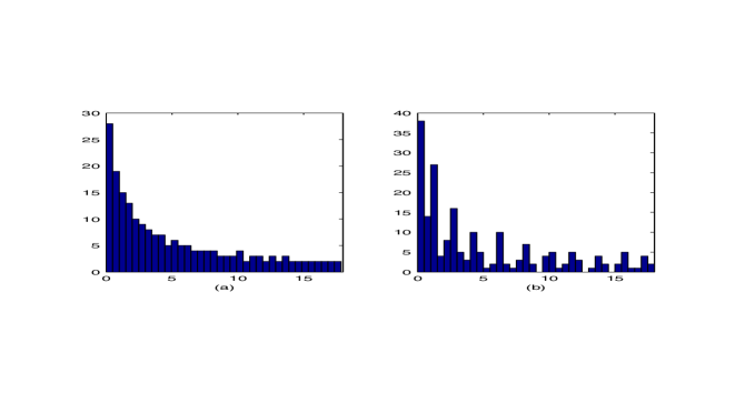
Example 6.4. As a final example we reran Example 6.1, but
using . The minimax
design had a relative efficiency of 1.17 against the best – the minbias
design – of the other three; the efficiency was much greater against the
uniform and saturated designs. See Table 2.
Figure 10: (a) Minbias design and (b) minimax () design for Example
6.4; both for .
Dette and Trampisch (2012) studied locally optimal quantile regression designs
for nonlinear models, and concluded with a call for future research into the
robustness of designs with respect to the model assumptions. In this article
we have detailed such research, with specific attention to linear models but
with an outline of the modest changes required to address nonlinear models.
Although a number of our methods described here are analytically and
numerically complex, some general guidance is possible. One recurring theme of
this article is that uniform designs are often minimax in
sufficiently large classes of the types of departures we consider. It has long
been recognized in problems of design for least squares regression that the
uniform design plays much the same role as does the median in robust
estimation – highly robust if not terribly efficient – and our findings seem
to extend this role to quantile regression.
In seeking protection against bias alone, resulting from model
misspecification and a particular variance function, designs with weights
proportional to the root of the variance function turn out to be minimax
against response misspecifications.
Uniform designs and minimum bias designs are easily implemented. The more
complex design strategies illustrated in §3 are
more laborious, but it has been seen that a rough description of the outcomes,
when there are already available non-robust designs which minimize the loss at
the experimenter’s assumed model, is that the robust designs can at least be
approximated by taking the replicates prescribed by the non-robust strategies,
and spreading these out into clusters of distinct but nearby design points.
The robust designs obtained here all yield substantial gains in efficiency, as
measured in terms of maximum loss, when compared to their competitors –
enough to warrant some computational complexity in their construction. As is
seen from the plots of the designs – Figures 1, 2,
6, 9 and 10 in particular
– a gain in efficiency should be realizable, without a great deal of
computation, by merely following the preceding heuristic of clustering
replicates, and combining this with design weights suggested by the minimum
bias paradigm.
Appendix: Derivations
Mathematical developments for
§3.1. With definitions , and
(14) becomes . We shall restrict to
variance functions for which we can verify that, evaluated at ,
(A.1)
We thus minimize , first with and fixed;
we then minimize over these values. For this we minimize , subject
to
(A.2)
It is sufficient that (i.e., all
elements non-negative) minimize the convex function
with the multipliers , pre-arranged in this convenient manner, chosen to satisfy the side
conditions. Since is a sum of univariate, convex functions it is
minimized over at the pointwise
positive part , where 0 is the stationary point of and . The calculations yield
(A.3)
with determined from (i), (ii) and (iii) of (A.2).
We may now minimize over rather than over , so that the numerical problem is
to minimize
with defined by (A.3)
and , , defined by (i), (ii) and (iii) of
(A.2). After doing this with a numerical constrained minimizer
we check (A.1). Then .
In Figure 1 we have illustrated only some representative variance
functions for which (A.1) holds. When it does not, one can minimize
instead and then check that, at the optimal design,
. If this also fails, then a more complex method which is however
guaranteed to succeed is that of Daemi and Wiens (2013), used in
§3.2.
We use methods introduced in Fang and Wiens (2000). We first represent the
design by a diagonal matrix with diagonal elements
. Define to be the
diagonal matrix with diagonal elements . Let be an matrix
whose columns form an orthogonal basis for the column space of the matrix
with rows – recall that this is ‘Q’ in the QR-decomposition of
. Then for a
, nonsingular triangular matrix . Augment
by whose columns
form an orthogonal basis for the orthogonal complement of this space. Then
is an orthogonal matrix and
is, by (i) of (8a), of the form
, where
. In these terms and from (B.8a) –
(B.8c),
Thus
Some algebra, followed by a return to the original parameterization, results
in (14).
Proof of Theorem 3. This
parallels the proof of Theorem 1 of Wiens (1992), and can also be obtained by
taking limits, as , in Theorem
2.
Derivation of (15). The, rather lengthy,
calculations for this section are available in Kong and Wiens (2014). As in
§3.1, we consider symmetric designs and
variance functions: and . In terms of
we define ,
and
We then calculate that
and that
whose characteristic roots are and the two
roots of
Of these two roots, one is uniformly greater than the other, and is
Thus the loss is , where .
We apply Theorem 1 of Daemi and Wiens (2013), by which we may proceed as
follows. We first find a density minimizing in the class of densities for which , and a density minimizing
in the class of densities for which
. Then the optimal
design has density
The two minimizations are first carried out with held fixed, thus fixing all and
. Under these constraints iff .
With the aid of Lagrange multipliers we find that both and are
of the form (15). The ten constants forming
are chosen to minimize the loss subject to the side conditions, but it is now
numerically simpler to minimize
at (14) directly over , subject to .
The density is overparameterized, and when is nonconstant we take . In the homogeneous case we
take and also and .
Proof of Proposition 1. We
give the proof of (i); that of (ii) is similar. For define
. Then
and note that , independently of . Thus it
suffices to show that for some ,
(A.4)
In fact serves the purpose. To see this note that by Proposition
1,
and that for any , , so that also . This establishes
(A.4) with .
Acknowledgements
This work has been supported by the Natural Sciences and Engineering Research
Council of Canada.
References
Behl, P., Claeskes, G, and Dette, H. (2014), “Focussed
Model Selection in Quantile Regression,” Statistica
Sinica, 24, 601-624.
Biedermann, S., and Dette, H. (2001), “Optimal Designs
for Testing the Functional Form of a Regression via Nonparametric Estimation
Techniques,” Statistics and Probability Letters,
52, 215-224.
Bischoff, W. (2010), “An Improvement in the Lack-of-Fit
Optimality of the (Absolutely) Continuous Uniform Design in Respect of Exact
Designs,” Proceedings of the 9th International
Workshop in Model-Oriented Design and Analysis (moda9), eds. Giovagnoli,
Atkinson, and Torsney, Springer-Verlag, Berlin Heidelberg.
Box, G. E .P., and Draper, N. R. (1959), “A Basis for
the Selection of a Response Surface Design,” Journal
of the American Statistical Association, 54, 622-654.
Cook, R. D., and Wong, W. K. (1994), “On the
Equivalence of Constrained and Compound Optimal Designs,” Journal of the American Statistical Association, 89, 687-692.
Daemi, M., and Wiens, D. P. (2013), “Techniques for the
Construction of Robust Regression Designs,” The
Canadian Journal of Statistics, 41, 679 - 695.
Dette, H., and Trampisch, M. (2012), “Optimal Designs
for Quantile Regression Methods,” Journal of the
American Statistical Association, 107, 1140-1151.
Fang, K. T., and Wang, Y. (1994), Number-Theoretic Methods in
Statistics, Chapman and Hall.
Fang, Z., and Wiens, D. P. (2000), “Integer-Valued,
Minimax Robust Designs for Estimation and Extrapolation in Heteroscedastic,
Approximately Linear Models,” Journal of the
American Statistical Association, 95, 807-818.
Hamill, P. V. V., Dridzd, T. A., Johnson, C. L., Reed, R. B., Roche, A.
F. and Moore, W. M. (1979), “Physical growth: National Center
for Health Statistics percentiles,” American Journal
of Clinical Nutrition, 32, 607-629.
Heo, G., Schmuland, B., and Wiens, D. P. (2001), “Restricted Minimax Robust Designs for Misspecified Regression
Models,” The Canadian Journal of Statistics, 29, 117-128.
Huber, P. J. (1964), “Robust Estimation of a Location
Parameter,” The Annals of Mathematical Statistics,
35, 73-101.
——– (1975), “Robustness and
Designs,” in: A Survey of Statistical Design and
Linear Models, ed. J. N. Srivastava, Amsterdam: North Holland, pp. 287-303.
——– (1981), Robust Statistics, New York: Wiley.
Kaishev, V. K. (1989), “Optimal Experimental Designs
for the B-spline Regression,” Computational
Statistics & Data Analysis, 8, 39-47.
Knight, K. (1998), “Limiting Distributions for
Estimators Under General Conditions,” Annals of
Statistics, 26, 755-770.
Koenker, R., and Bassett, G. (1978), “Regression
Quantiles,” Econometrica, 46, 33-50.
Koenker, R. (2005), Quantile Regression. Cambridge University
Press.
Kong, L., and Mizera, I. (2012), “Quantile Tomography:
Using Quantiles with Multivariate Data,” Statistica
Sinica, 22, 1589-1610.
Kong, L., and Wiens, D. P. (2014), “Robust Quantile
Regression Designs,” University of Alberta
Department of Mathematical and Statistical Sciences Technical Report S129,
http://www.stat.ualberta.ca/~wiens/home page/pubs/TR S129.pdf.
Li, K .C. (1984), “Robust Regression Designs When the
Design Space Consists of Finitely Many Points,” The
Annals of Statistics, 12, 269-282.
Li, P., and Wiens, D. P. (2011), “Robustness of Design
for Dose-Response Studies,” Journal of the Royal
Statistical Society (Series B), 17, 215-238.
Ma, Y., and Wei, Y. (2012), “Analysis on Censored
Quantile Residual Life Model via Spline Smoothing,” Statistica Sinica, 22, 47-68.
Maronna, R. A., and Yohai, V. J. (1981), “Asymptotic
Behaviour of General M-Estimates for Regression and Scale With Random
Carriers,” Zeitschrift für
Wahrscheinlichkeitstheorie und Verwandte Gebiete, 58, 7-20.
Martínez-Silva, I., Roca-Pardiñas, J., Lustres-Pérez, V.,
Lorenzo-Arribas, A., and Cadaro-Suárez, C. (2013), “Flexible Quantile Regression Models: Application to the Study of the Purple
Sea Urchin,” SORT, 37, 81-94.
Pere, A. (2000), “Comparison of Two Methods of
Transforming Height and Weight to Normality,” Annals
of Human Biology, 27, 35-45.
Pollard, D. (1991), “Asymptotics for Least Absolute
Deviation Regression Estimators,” Econometric
Theory, 7, 186-199.
Rubia, A., Sanchis-Marco, L. (2013), “On Downside Risk
Predictability Through Liquidity and Trading Activity: A Dynamic Quantile
Approach,” International Journal of Forecasting,
29, 202-219.
Shi, P., Ye, J., and Zhou, J. (2003), “Minimax Robust
Designs for Misspecified Regression Models,” The
Canadian Journal of Statistics, 31, 397-414.
Simpson, D. G., Ruppert, D., and Carroll, R. J. (1992),
“On One-Step GM Estimates and Stability of Inferences in
Linear Regression,” Journal of the American
Statistical Association, 87, 439-450.
Wei, Y., and He, X. (2006), “Discussion Paper:
Conditional Growth Charts,” Annals of Statistics,
34, 2069-2097.
Wei, Y., Pere, A., Koenker, R., and He, X. (2006), “Quantile Regression Methods for Reference Growth Charts,” Statistics in Medicine, 25, 1369-1382.
Welsh, A. H. and Wiens, D. P. (2013), “Robust
Model-based Sampling Designs,” Statistics and
Computing, 23, 689-701.
Wiens, D. P. (1991), “Designs for Approximately Linear
Regression: Two Optimality Properties of Uniform Designs,” Statistics and Probability Letters; 12, 217-221.
——– (1992), “Minimax Designs for Approximately
Linear Regression,” Journal of Statistical Planning
and Inference, 31, 353-371.
——– (2000), “Robust Weights and Designs for Biased
Regression Models: Least Squares and Generalized
M-Estimation,” Journal of Statistical Planning and
Inference, 83, 395-412.
——–, and Wu, E. K. H. (2010), “A Comparative Study
of Robust Designs for M-Estimated Regression Models,” Computational Statistics and Data Analysis, 54, 1683-1695.
Woods, D.C., Lewis, S.M., Eccleston, J. A., and Russell, K. G. (2006),
“Designs for Generalized Linear Models with Several
Variables and Model Uncertainty”, Technometrics,
48, 84–292.
Xu, X., and Yuen, W. K. (2011), “Applications and
Implementations of Continuous Robust Designs,” Communications in Statistics - Theory and Methods, 40, 969-988.
University of Alberta
Department of Mathematical and Statistical Sciences
Technical Report S129
ROBUST QUANTILE REGRESSION DESIGNS
Linglong Kong and Douglas P. Wiens222Department of Mathematical and Statistical
Sciences; University of Alberta, Edmonton, Alberta; Canada T6G 2G1. e-mail:
lkong@ualberta.ca, doug.wiens@ualberta.ca
Abstract This technical report contains unpublished
material, relevant to the article ‘Model-Robust Designs for Quantile
Regression’.
where is the ‘check’ function , with
derivative . Define
the target parameter to be the asymptotic solution to
(B.6), so that
(B.7)
in agreement with (B.5). We require the following conditions.
(A1)
The distribution function defined on is twice continuously differentiable. The density
is everywhere finite, positive and Lipschitz continuous.
(A2)
(A3)
There exists a vector , and positive definite
matrices and , such that,
with ,
Recall the definitions
(B.8a)
(B.8b)
(B.8c)
Assume that the support of is large enough that and are positive definite. We have:
Theorem 4
Under conditions (A1) – (A3) the quantile
regression estimate of the parameter
defined by (B.7) is asymptotically normally
distributed:
(B.9)
Proof Here we write an -point design as , with the not necessarily distinct. We first show that
(B.10)
For this, define , where and . The function is convex
and is minimized at . The main idea of the proof
follows Knight (1998). Using Knight’s identity
we may write , where
and . We note that
and that
It follows from the Lindeberg-Feller Central Limit Theorem, using Condition
(A3), that where. Now centre :
We have
As well, we have the bound
Condition (A2) implies that var. As a consequence, and
.
Combining these observations, we have
The convexity of the limiting objective function
ensures the uniqueness of the minimizer, which is . Therefore, we have
(B.11)
Similar arguments can be found in Pollard (1991) and Knight (1998). From
(B.11) we immediately obtain (B.10).
To go from (B.10) to (B.9) requires passing from the
limits in (A3) to (B.8). The expansion
yields . Here we
require to
be bounded; this is implied by the existence of :
Similarly, the expansion gives that
Finally, the expansion gives
Appendix B Variance functions
- additional examples
We consider classes of variance functions given by
(B.12c)
(B.12f)
in discrete and continuous spaces respectively. When the experimenter seeks
protection against a fixed alternative to homoscedasticity,
i.e. fixed , some cases of (B.12) may be treated in generality.
B.1 Discrete designs for variance functions (B.12) with
fixed
Example 2.1. If then and
(B.14)
Without some restriction on the class of designs so as to make it compact,
there are sequences of designs for which
tends to the minimum value of
(B.14) as , but has one-point support, so
that is singular. To see this, define . Since
and
, we have that . If places mass
at an for which is attained, and mass
at every other point , then
and so as
. This degeneracy can be avoided by, for instance, imposing
a positive lower bound on the non-zero design weights.
B.2 Continuous designs for variance functions (B.12f)
with fixed
Example 2.1 continued. If then and
As in the discrete version of this example, a degenerate solution can be
avoided at the cost of imposing superfluous restrictions on the
designs.
Example 2.2 . The case and results in
The optimal design is uniform, with density vol. To prove this we note
that it is sufficient to show that . This is established by introducing and then using Proposition 1 to
obtain .
Appendix C Calculations for the construction of continuous minimax
designs for quadratic regression and fixed variance functions
We consider symmetric designs and variance functions: and
. In terms of
we have that
and
Define . Then
hence (replacing by in the above)
Then
We have that
which we represent as
where and
Note that in this notation
The characteristic roots of are and the two characteristic roots of
Of these two roots, one is uniformly greater than the other, and is
Thus the loss is the greater of
We apply Theorem 1 of Daemi and Wiens (2013), by which we may proceed as
follows. We first find a density minimizing in the class of densities for which , and a density minimizing
in the class of densities for which
. Then the optimal
design has density
The two minimizations are first carried out with held fixed, thus fixing all and
. Under these constraints iff . We first illustrate the calculations for .
We seek
where is a slack variable. For densities , and
with
it is sufficient to find for which the Lagrangian
is minimized at for every and satisfies the
side conditions. The first order condition is
where is a slack variable. For densities , and
with
it is sufficient to find for which the Lagrangian
is minimized at for every and satisfies the
side conditions. This leads to the same first order condition as
(B.15), except that is replaced by ;
this in turn leads to
In either case, the minimizing design density is of the form
(B.16)
for polynomials ,
. The constants forming are determined by the
constraints in terms of the , and , which are
then optimally chosen to minimize the loss. It is simpler however to choose
directly, to minimize over all densities of the form (B.16), subject to
.
Acknowledgements
This work has been supported by the Natural Sciences and Engineering Research
Council of Canada.
References
Daemi, M., and Wiens, D. P. (2013), “Techniques for the
Construction of Robust Regression Designs,” The
Canadian Journal of Statistics, 41, 679 - 695.
Knight, K. (1998), “Limiting Distributions for
Estimators Under General Conditions,” Annals of
Statistics, 26, 755-770.
Pollard, D. (1991), “Asymptotics for Least Absolute
Deviation Regression Estimators,” Econometric
Theory, 7, 186-199.