Complete spectrum of the infinite-$U$ Hubbard ring using group theory

Abstract

We present a full analytical solution of the multiconfigurational strongly-correlated mixed-valence problem corresponding to the $N$-Hubbard ring filled with $N-1$ electrons, and infinite on-site repulsion. While the eigenvalues and the eigenstates of the model are known already, analytical determination of their degeneracy is presented here for the first time. The full solution, including degeneracy count, is achieved for each spin configuration by mapping the Hubbard model into a set of Hückel-annulene problems for rings of variable size. The number and size of these effective Hückel annulenes, both crucial to obtain Hubbard states and their degeneracy, are determined by solving a well-known combinatorial enumeration problem, the necklace problem for $N-1$ beads and two colors, within each subgroup of the ${\mathbf{C}}_{N-1}$ permutation group. Symmetry-adapted solution of the necklace enumeration problem is finally achieved by means of the subduction of coset representation technique [S. Fujita, Theor. Chem. Acta 76, 247 (1989)], which provides a general and elegant strategy to solve the one-hole infinite-$U$ Hubbard problem, including degeneracy count, for any ring size. The proposed group theoretical strategy to solve the infinite-$U$ Hubbard problem for $N-1$ electrons, is easily generalized to the case of arbitrary electron count $L$, by analyzing the permutation group ${\mathbf{C}}_{L}$ and all its subgroups.

I Introduction

It is a well-established fact that the electronic structure of systems containing $d$ and $f$ electrons is poorly modelled by single-determinant approximations. Well-known examples in solid state physics are Mott insulators,Mott1968 wrongly predicted to be metals within an independent particle picture. In molecular science, strong electron correlation and multiconfigurational electronic states play a central role in the description of the rich magnetic behavior of polynuclear inorganic complexes of transition metal and rare earth ions with partially filled $d$ and $f$ angular momentum shells, also known as molecular nanomagnets.Gatteschi2006 Despite the advances of multiconfigurational ab initio methods such as CASSCF/CASPT2, first principles approaches are to date still too demanding to describe complexes involving more than one or two metal ions. In this scenario, simple models of electron correlation can be very helpful, both to provide interpretation of ab initio results, or to tackle large electronic structure problems.

One widely used multiconfigurational atomistic model of strongly electron-correlated systems is the Hubbard model.EsslerBook2005 ; Tasaki1998a ; Tasaki1998b In its original formulation it provides a description of a set of $L$ active electrons occupying $N$ orthogonal orbitals localized on $N$ metal atoms. The simplest Hubbard Hamiltonian reads:

$$H=t\sum_{\langle ij\rangle}\sum_{\sigma}^{\uparrow\downarrow}c_{i\sigma}^{\dagger}c_{j\sigma}+U\sum_{i}^{N}n_{i\uparrow}n_{i\downarrow}$$ (1)

where according to the usual notation $c_{i\sigma}^{\dagger}$ and $c_{i\sigma}$ are the creation and annihilation operators for electrons occupying the atomic orbital at site $i$ with spin $\sigma$, and $n_{i\sigma}=c^{\dagger}_{i\sigma}c_{i\sigma}$, and the angular parenthesis limits summation over nearest-neighbors . The two fundamental ingredients in the basic Hubbard Hamiltonian are the charge transfer term $H_{t}$ between nearest neighbor sites (first term on the right hand side of Eq. (1)), here parametrized by the hopping integral $t$, and the on-site Coulomb repulsion term, here parametrized by the two-electron repulsion integral $U>0$.

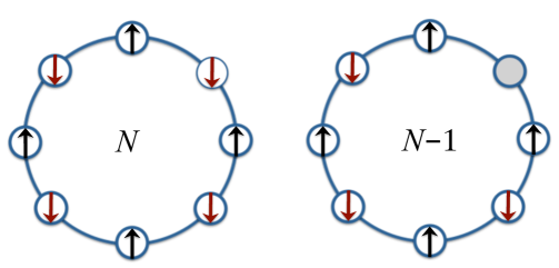
Figure 1: Scheme of a Hubbard ring with $N$ metal centers and $N$ electrons (left) or $N-1$ electrons (right). The constraint $U=\infty$ implies that each orbital is occupied at most by one electron, and thus all electronic configurations describing the multiconfigurational states of the $N-1$ Hubbard ring will always involve a single empty orbital (shaded-atom).

I.1 Mixed-valence one-hole Hubbard ring

Despite its apparent simplicity, exact solutions to Eq. (1) are known for very few connectivities. One well-known case is that of 1-dimensional systems, also known as Hubbard rings, representing an important electron correlation model for e.g. molecular wheel nanomagnets. The Hubbard ring problem can be solved exactly either via the Bethe ansatz, or in the case of infinite U, also via a particular unitary transformation of the basis states. Here we will be interested in the infinite U case, which represents an approximation to the strong coupling limit. Although the expression for the eigenvalues of the Hubbard ring with infinite U and arbitrary filling is known,Caspers1989 ; Kotrla1990 to the best of our knowledge the exact degeneracy of each solution has never been addressed in the literature.

Two particular electron-counts are clearly of greater relevance, as these counts are more likely to represent chemically stable charge-states of molecular metal rings: the half-filling electron count ($N$ electrons on $N$ metal centers, see Fig. 1 left), and the half-filling minus one electron count ($N-1$ electrons on $N$ metal centers, see Fig. 1 right). Note that the half-filling plus one ($N+1$ electrons) is obtained from the $N-1$ case simply by changing the sign of the hopping integral $t$.

The first case (half-filling) is uninteresting in the limit of infinite U, as then all $2^{N}$ Slater determinants have the same energy, since no hopping process is permitted by the infinite value of U. In fact the half-filling case in the limit of large but finite U can be discussed also within a perturbative approach, where the hopping part of the Hamiltonian couples the $2^{N}$ degenerate determinants arising from single occupation of the orbital, with charge transfer configurations in which one orbital is doubly occupied and another remains empty. The inclusion of the effect of the high-energy charge-transfer configurations to second order in $t$ leads to the mapping of the Hubbard ring problem for half-filling into the Heisenberg ring problem with spin one-half on site.Tasaki1998b

More interesting is the second case ($N-1$ electrons) in the limit of infinite U. This model represents the simplest description of the electron correlation problem arising in a mixed-valence metal ring, where one metal contributes no valence electrons, while all the others contribute one electron. For instance, singly oxidized (and singly reduced) infinite-$U$ Hubbard rings can be used to describe states that are relevant for quantum transport in molecular rings devices in the Coulomb-blockade regime, BruusFlensberg2004 ; ElsteTimm2005 as conduction via such rings is described by electrodes-induced transitions between the states of the half-filled ring, and those of the singly oxidized or singly reduced ring, with the extra electron occupying an empty atomic orbital centred at a metal’s site. SonciniJACS2010 ; SonciniPRB2010

In this paper we show that the Hubbard $N$-ring for $N-1$ electron filling can be solved exactly by mapping it into a set of Hückel annulene problems for which the analytical spectrum is well known once the size of the ring is known. Thus once the number $N$ of metal centers in the Hubbard ring is known and the total number of spin-up electrons in the ring is fixed, the only problem that remains to be solved is to determine what are the sizes of the associated Hückel rings, and how many Hückel rings of a given size are there. This problem will be solved with the aid of group theory. Finally, we will show that our group theory strategy to count the repetition of the same effective Hückel spectrum in the solution of the $N-1$ Hubbard problem can also be applied to count analytical solutions for any electron filling of the ring.

II Mapping of the one-hole Hubbard ring problem into a collection of Hückel problems

The Hubbard Hamiltonian Eq. (1) can be simplified for a metal ring with $N$ sites as

$$H=t\sum_{i=1}^{N}\sum_{\sigma=\uparrow,\downarrow}(c^{\dagger}_{i+1,\sigma}c_{i,\sigma}+c^{\dagger}_{i,\sigma}c_{i+1,\sigma})+U\sum_{i=1}^{N}n_{i,\uparrow}n_{i,\downarrow},$$ (2)

where cyclic boundary conditions are imposed by identifying site $N+1$ with site 1. The ring is occupied with $L\leq 2N$ electrons. The solutions for $L>N$ electrons are obtained easily from the solutions for $2N-L$ electrons by replacing $t$ with $-t$ everywhere (this is the hole-particle transformation). We will therefore consider the $L\leq N$ cases only.

When $U=0$, Eq. (2) trivially reduces to the Hamiltonian of a Hückel cycle with $L$ noninteracting electrons, whose well-known eigenstates consist of single Slater determinants with energy

$$E=2t\sum_{\lambda}^{\mathrm{occ}}\cos\frac{2\pi\lambda}{N},$$ (3)

where the sum runs over the $L$ occupied molecular Hückel orbitals, labeled by the quantum number $\lambda$, which can be interpreted as an effective orbital angular momentum component along the rotational $C_{N}$ axis of symmetry SteinerFowlerJPCA2001 ; SteinerFowlerChemComm2001 (and also representing an irreducible representation of the molecular symmetry group ${\mathbf{C}}_{N}$). The angular momentum $\lambda$ can take the following values:

$$\lambda =0,\pm 1,\pm 2,\ldots,\pm(N-1)/2 N$$ for odd (4)

$$\lambda =0,\pm 1,\pm 2,\ldots,\pm(N/2-1),\,N/2 \text{for $N$ even}.$$ (5)

When $U>0$, the problem becomes multiconfigurational and the solutions are in general not so easy to find. However, in the limit of strong on-site repulsion $U\rightarrow\infty$, the only relevant Slater determinants are those representing an electronic configuration in which each site-orbital is either empty or singly occupied (see Figure 1 on the right). In this case several useful statements can be made about the block-diagonal structure of the Hamiltonian matrix in the basis of this particular subset of Slater determinants.

Each of these determinants can in fact be specified completely by the row vectors $\mathbf{x}=(x_{1},x_{2},\ldots,x_{L})$, listing the occupied sites (in increasing order), and $\bm{\sigma}=(\sigma_{1},\sigma_{2},\ldots,\sigma_{L}$), listing the corresponding spin values, as follows:

$$|\mathbf{x},\bm{\sigma}\rangle=c^{\dagger}_{x_{1},\sigma_{1}}c^{\dagger}_{x_{2},\sigma_{2}}\ldots c^{\dagger}_{x_{L},\sigma_{L}}|0\rangle,\qquad 1\leq x_{1}<x_{2}<\ldots<x_{L}\leq N$$ (6)

In this work we will focus mainly on the $N-1$-electron count, and for this specific case it is possible to classify the one-hole determinant basis states in terms of the position of the single empty orbital $l$ ($l=1,\dots,N$), and the spin configuration $\bm{\sigma}=\{\sigma_{i}\}_{i\neq l}$ for the $N-1$ sites. Thus we write the basis of one-hole Slater determinants as:

$$|l,\bm{\sigma}\rangle=(-1)^{l-1}\prod_{\begin{subarray}{c}i=1\\ i\neq l\end{subarray}}^{N}c^{\dagger}_{i,\sigma_{i}}|0\rangle.$$ (7)

We note that this phase choice has the advantage that the matrix elements of $H_{t}$ in this basis are equal either to $-t$ or to zero.Tasaki1998a Each of these states is also characterized by its value of $M_{S}=(n_{1}-n_{2})/2$, where $n_{1}$ ($n_{2}$) is the number of spin-up (down) electrons in $\bm{\sigma}$. Both $M_{S}$ and the total spin $S$ are conserved quantities. Within this space we must now diagonalize the hopping Hamiltonian $H_{t}$ (first part of Eq. (2)). Under the action of $H_{t}$ a spin can hop to a neighboring site only if that site is empty.

Since double occupations are never allowed, it follows that in a one-dimensional nearest-neighbor connectivity the ordering of a given sequence of spin-up/spin-down polarizations in $\bm{\sigma}$ will be conserved under the action of $H_{t}$. We will also refer to this $\bm{\sigma}$-ordering as spin configuration. This simple observation has a few crucial consequences:

• Within a given $M_{S}$ subspace of Slater determinants, $H_{t}$ will be block-diagonal in the spin configuration vector $\bm{\sigma}$.

• The matrix-structure of each $\bm{\sigma}$-block is in fact that of the Hückel Hamiltonian matrix for a $n_{\sigma}$-annulene, with hopping integrals $\beta=-t$. This can be easily seen by repeated application of $H_{t}$ to an initial one-hole Slater determinant, generating a full closed orbit (Hückel annulene) of $n_{\sigma}$ Slater determinants, where each determinant is only connected by $H_{t}$ to two other determinants: one where the hole is one position back, and the other where the hole is one position forward (see Fig. 2, illustrating the case of 2 electrons in a 3-center Hubbard ring with $M_{S}=0$, mapped into an $n_{\sigma}$-annulene with $n_{\sigma}=6$, i.e. into Hückel benzene). Note that for electron counts different from $N-1$, $H_{t}$ still generates a closed orbit of Slater determinants for each given spin configuration $\bm{\sigma}$, although the matrix connectivity of the graph associated to such orbit will not be a simple ring connectivity.

• The N-sites Hubbard ring eigenvalues obtained from each block are thus coincident with those of a Hückel annulene problem with $n_{\sigma}$ sites, and read $\epsilon=-2t\cos\frac{2\pi\lambda}{n_{\sigma}}$, with $\lambda=0,\pm 1,\pm 2,\dots\frac{n_{\sigma}}{2}$ (if $n_{\sigma}$ is even), or $\pm\frac{(n_{\sigma}-1)}{2}$ (if $n_{\sigma}$ is odd).

Hence, the infinite-$U$ Hubbard ring problem is fully diagonalized provided we can (i) enumerate all the independent Hückel rings (i.e. spin configurations $\bm{\sigma}$ ), for every given $M_{S}$, and (ii) determine the size $n_{\sigma}$ of each Hückel ring (i.e. the size of the orbit of Slater determinants with same spin configuration $\bm{\sigma}$, generated by repeated application of the hopping Hamiltonian $H_{t}$). We show below how this can be simply achieved for small rings, but quickly becomes a non trivial counting problem that needs be approached via the powerful techniques of group theory.

II.1 Two electrons in three orbitals: Hubbard 3-ring mapped into Hückel benzene

Let us at first consider the smallest Hubbard ring, with $N=3$ and the non-trivial total spin projection $M_{S}=0$. We have here two electrons of opposite spin polarization hopping over three metal-centered orbitals.

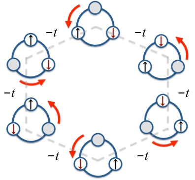
Figure 2: The clockwise hopping of two electrons in three orbitals defines an $M_{S}=0$ space of six Slater determinants cyclically connected by hopping integral $-t$. Note that this is equivalent to the anticlockwise hopping of the empty site around the ring, although the starting configuration can only be obtained after two turns of the Hubbard ring, turning the 3-ring into a 6-cycle. Within the determinant basis space, the Hubbard Hamiltonian is thus mapped into a Hückel benzene, which can be analytically diagonalized (see text).

For this simple example it is clear that only one orbit of Slater determinants exists. It is in fact interesting to note that the hopping of one electron e.g. in a clockwise direction formally corresponds to the hopping of the empty orbital in the opposite (anticlockwise) direction, as illustrated in Figure 2.

Note also that the empty orbital needs to hop twice around the 3-membered ring in order for the hopping Hamiltonian $H_{t}$ to span the whole orbit of Slater determinants, so that the size of this orbit for the spin configuration $\bm{\sigma}=(\uparrow,\downarrow)$ is $n_{\uparrow\downarrow}=3\times 2=6$. As anticipated in the previous paragraph, and shown here in Figure 2, if the 6-dimensional determinant basis is ordered according to consecutive hopping processes, each of the six configurations is connected by $H_{t}$ only to its two nearest neighbor determinants, so that hopping defines a ring of Slater determinants which has double the size of the Hubbard ring. The resulting block of the infinite-$U$ Hubbard Hamiltonian clearly reads:

$$H_{\uparrow\downarrow}=\left(\begin{array}[]{cccccc}0&-t&0&0&0&-t\\ -t&0&-t&0&0&0\\ 0&-t&0&-t&0&0\\ 0&0&-t&0&-t&0\\ 0&0&0&-t&0&-t\\ -t&0&0&0&-t&0\end{array}\right)$$ (8)

which is equivalent to the Hückel Hamiltonian for benzene. Thus $H_{t}$ is easily diagonalized within the $M_{S}=0$ subspace, leading to a spectrum with the six eigenvalues $\epsilon_{\lambda}^{\uparrow\downarrow}=-2t\cos(\frac{2\pi\lambda}{6})$, for $\lambda=0,\pm 1,\pm 2,3$. As for the triplet projections $M_{S}=1$, the matrix representation of $H_{t}$ can be mapped into a Hückel $[3]$-annulene, with the three eigenvalues $\epsilon_{\lambda}^{\uparrow\uparrow}=-2t\cos(\frac{2\pi\lambda}{3})$, $\lambda=0,\pm 1$. Note that if $t>0$, the ground state is high-spin (triplet), as expected for rings with $N=3$ and $N=4$, where Nagaoka’s theorem is fulfilled.Tasaki1998a

II.2 Four electrons in five orbitals with $M_{S}=0$: multiple orbits / Hückel annulenes

The case of four electrons in a Hubbard ring with five metal centers represents the smallest 1D-Hubbard problem for which we encounter multiple orbits/spin configurations within a given value of $M_{S}$. In the case $M_{S}=0$ we can build two families of Slater determinants, one corresponding to an alternating spin configuration $\bm{\sigma}_{1}=(\uparrow,\downarrow,\uparrow,\downarrow)$ , the other $\bm{\sigma}_{2}=(\uparrow,\uparrow,\downarrow,\downarrow)$, as illustrated in Figure 3. It is evident that these two families of determinants cannot be connected via simple hopping process. Thus the $M_{S}=0$ subspace is further block-diagonalized into two subspaces, each subspace corresponding to a different orbit.

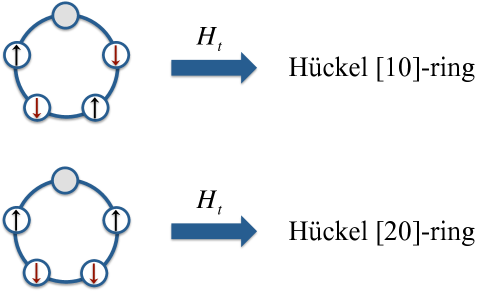
Figure 3: The two orbits of spin determinants representing two separate subspaces within the $M_{S}=0$ spin projection space, for four electrons in five orbitals. Note that these two orbits of spin configurations under the action of the hopping Hamiltonian $H_{t}$ generate an adjacency matrix for two distinct Hückel rings, one with ten vertices, the second with 20 vertices.

In particular, by repeatedly applying the hopping Hamiltonian $H_{t}$ to any determinant with spin configuration $\bm{\sigma}_{1}$ (top of Figure 3), the hole has to hop twice around the 5-Hubbard ring to get back to starting configuration, so that the length of this orbit is $n_{\uparrow\downarrow\uparrow\downarrow}=2\times 5=10$. The block $\bm{\sigma}_{1}$ of the Hubbard Hamiltonian is thus mapped into the eigenvalue problem for the Hückel [10]-ring, with spectrum $\epsilon_{\lambda}^{\uparrow\downarrow\uparrow\downarrow}=-2t\cos(\frac{2\pi\lambda}{10})$, $\lambda=0,\pm 1,\pm 2,\pm 3,\pm 4,5$. On the other hand, it can be seen by direct inspection that the full orbit of determinants corresponding to the spin configuration $\bm{\sigma}_{2}$ (bottom of Figure 3) can be generated if the hole hops four times around the 5-Hubbard ring, so that $n_{\uparrow\uparrow\downarrow\downarrow}=4\times 5=20$. The Hubbard block $\bm{\sigma}_{2}$ is thus equivalent to the Huc̈kel Hamiltonian for a [20]annulene, with spectrum $\epsilon_{\lambda}^{\uparrow\downarrow\downarrow\uparrow}=-2t\cos(\frac{2\pi\lambda}{20})$, $\lambda=0,\pm 1,\pm 2,\dots,\pm 9,10$.

III Mapping the Hückel annulenes enumeration problem into a necklace enumeration problem

From the previous examples we note that the size of the Hückel annulenes associated to the $\bm{\sigma}$-blocks is always an integer multiple of the number of metal centers $N$ in the Hubbard ring, as the hole must always hop in units of $N$-steps to get back to the initial site and close the spin-configuration orbit. The problem is to find how many times the hole has to hop around the Hubbard ring in order to span the full orbit. For small Hubbard rings, it is easy enough to work this out by inspection. However, the problem becomes increasingly tedious as $N$ becomes larger.

A systematic strategy to enumerate Hückel annulenes and determine their sizes for each given $M_{S}$ is offered by group theory. The connection between enumeration of orbits of Slater determinants / Hückel annulenes, and group theory, can be readily made by noting that after each single turn of the empty orbital around the Hubbard ring, the spin configuration $\bm{\sigma}$ undergoes a cyclic permutation within the remaining $N-1$ occupied sites.

If all $N-1$ occupied sites have parallel spins ($|M_{S}|=(N-1)/2$ ), the cyclically permuted spin configuration is indistinguishable from the initial spin configuration, thus a single turn of the empty orbital around the Hubbard ring suffices to generate a full orbit of Slater determinants, and the associated Hückel ring has the same size as the Hubbard ring (i.e. $n_{\sigma}=N$). This implies that the spectrum of the $N$-Hubbard ring with $N-1$ electrons for $|M_{S}|=(N-1)/2$ corresponds to the Hückel spectrum of an $[N]$-annulene with resonance integral $\beta=-t$. The eigenvalues are therefore $\epsilon_{\lambda}=-2t\cos\left(\frac{2\pi\lambda}{N}\right)$, with $\lambda=0,\pm 1,\dots,N/2$ if $N$ is even, or $\pm(N-1)/2$ if N is odd. Beside the pure spin $\pm M_{S}$ double degeneracy, these states present additional orbital double-degeneracies associated to the axial orbital angular momentum quantum number $\pm\lambda$, as it is found in common Hückel $[N]$-annulenes.

For $|M_{S}|<(N-1)/2$, the cyclically permuted spin configuration $\bm{\sigma}$ generated by $N$ hopping processes is not equivalent to the initial spin configuration. The effect of $N$-hopping processes on a one-hole determinant is thus equivalent to the action of the cyclic permutation $\hat{C}_{N-1}$ (generator of the permutation group ${\mathbf{C}}_{N-1}$) on a two-color necklace with $N-1$ beads, where a given bead has color X (Y) if the corresponding occupied site in the Hubbard ring has spin up (down). The two-colored necklace is in fact a representation of the spin-ordered configuration $\bm{\sigma}$ under scrutiny, where the ratio between the number of beads with different color is fixed by the value of $M_{S}$.

Crucially, the problem of enumerating $\bm{\sigma}$ spin configurations for a given $M_{S}$ that are not connected by hopping processes (i.e. enumerating Hückel annulenes), is now mapped into the well-known combinatorial problem of enumerating symmetry-unique (i.e. not related by cyclic permutations) necklaces with $N-1$ beads of two colors, with a fixed ratio between beads of different colors. Furthermore, grouping together all necklaces of like symmetry, that is all distinguishable necklaces that can be rotated into each other by repeated application of a cyclic permutation $\hat{C}_{N-1}$, we obtain orbits of two-color necklaces with size $\omega_{\sigma}$. The length of each Hückel annulene associated with a fixed $M_{S}$ Hubbard problem can now be found by determining the length $\omega_{\sigma}$ of the associated necklace-orbit generated by the action of the cyclic permutation group ${\mathbf{C}}_{N-1}$ on a representative necklace configuration. Once the length of each necklace orbit has been determined, the size of the associated Hückel ring $n_{\sigma}$, thus the corresponding set of Hubbard eigenvalues, is easily determined as:

$$n_{\sigma}=N\times\omega_{\sigma}$$ (9)

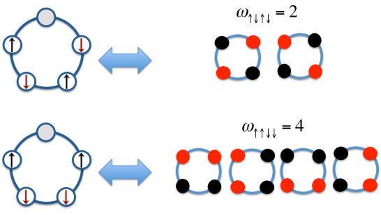
Figure 4: The two 4-beaded necklace orbits associated with the two spin configurations spanning the $M_{S}=0$ spin projection space, for the infinite-$U$ Hubbard problem of four active electrons in five orbitals. The necklace orbit-length is reported as $\omega_{\sigma}$. To obtain the full Slater determinant orbit length (hence the length of the associated Hückel rings) the necklace orbit length $\omega_{\sigma}$ must be multiplied by the number of metal centers (i.e. by five in this case), as detailed in Eq. (9).

To illustrate the mapping of the Hückel annulenes enumeration problem, into a necklace enumeration problem, let us consider the two Slater determinant orbits found in the previous section for the case of four electrons in five active orbitals (see also Figure 3). The mapping process is shown in Figure 4, where beads of color X and Y are represented by black and red beads. Here we have $N-1=4$, so we start off with a 4-beaded necklace which has full permutation symmetry ${\mathbf{C}}_{4}$ if all beads have the same color ($|M_{S}|=2$). For the $M_{S}=0$ space, the two spin configurations $\bm{\sigma}_{1}=(\uparrow,\downarrow,\uparrow,\downarrow)$ and $\bm{\sigma}_{2}=(\uparrow,\uparrow,\downarrow,\downarrow)$ identified in the previous paragraph can now be mapped into two symmetry-unique necklace configurations, with two black beads, and two red beads. In fact, decoration of the ${\mathbf{C}}_{4}$ necklace backbone with beads of two different colors can only lead to necklaces whose symmetry is described by a subgroup of ${\mathbf{C}}_{4}$. The group ${\mathbf{C}}_{4}$ has three subgroups : ${\mathbf{C}}_{4}$, ${\mathbf{C}}_{2}$ and ${\mathbf{C}}_{1}$ (i.e. no symmetry). By inspection, it is clear that the necklace associated to $\bm{\sigma}_{1}=(\uparrow,\downarrow,\uparrow,\downarrow)$ (top of Figure 4) has permutation symmetry ${\mathbf{C}}_{2}$, while the necklace associated to $\bm{\sigma}_{2}=(\uparrow,\uparrow,\downarrow,\downarrow)$ has symmetry ${\mathbf{C}}_{1}$.

The size of the necklace orbits can be easily found by inspection in this case. If we consider the four symmetry operations of the group ${\mathbf{C}}_{4}=\left\{\hat{E},\hat{C}_{4},\hat{C}_{4}^{2}\equiv\hat{C}_{2},\hat{C}_{4}^{3}\right\}$, by definition the necklace with symmetry ${\mathbf{C}}_{2}$ will be invariant with respect to the action of identity and $\hat{C}_{4}^{2}\equiv\hat{C}_{2}$, and will only be rotated into a distinguishable configuration under the action of $\hat{C}_{4}$. The orbit is consequently composed of two configurations only ($\omega_{\sigma_{1}}=2$, see top of Figure 4). On the other hand, the necklace with symmetry ${\mathbf{C}}_{1}$ will be rotated into four symmetry-related but distinguishable necklaces by the action of ${\mathbf{C}}_{4}$, thus generating an orbit of size $\omega_{\sigma_{2}}=4$ (see bottom of Figure 4). According to Eq. (9), the size of the corresponding Hückel annulenes can then be found as $n_{\sigma_{1}}=5\times\omega_{\sigma_{1}}=10$, and $n_{\sigma_{2}}=5\times\omega_{\sigma_{2}}=20$.

This reasoning can be made more rigorous within group theory, by exploring the relationship between groups, subgroups and orbits. It is in fact well known that in a structure with a given symmetry group (e.g. a molecule), orbits of symmetry-related points (e.g. atoms, atomic orbitals, bonds, etc.) can be fully characterised in terms of those subgroups describing the site or local symmetry of these points. Burnside1911 ; Fujita1989 Group/subgroup relationships describing orbits in molecular graphs have been used to characterise fundamental chemical and physical properties of molecules. FowlerQuinn1986 ; Fujita1989 ; CeulemansFowler1991

More specifically, given a high-symmetry structure described by the group ${\mathbf{G}}$, there is a well-defined link between (i) the symmetry descent from ${\mathbf{G}}$ to one of its subgroups ${\mathbf{G}}_{k}$ describing symmetry-lowering of the structure upon decoration (${\mathbf{G}}_{k}$ plays the role of a site-symmetry), and (ii) the size of the orbits generated by the action of the higher symmetry group ${\mathbf{G}}$ on the lower-symmetry decorated structures. In particular, the size of the orbit spanned by the ${\mathbf{G}}_{k}$-symmetry decorated structures, is simply the ratio between the number of elements in the higher group generating the orbit (order $|{\mathbf{G}}|$ of the higher group), and the order $|{\mathbf{G}}_{k}|$ of the subgroup. In brief, $\omega_{k}=|{\mathbf{G}}|/|{\mathbf{G}}_{k}|$. In this case, since ${\mathbf{C}}_{4}$ has order 4, ${\mathbf{C}}_{2}$ has order 2, and ${\mathbf{C}}_{1}$ has order 1, it follows that $\omega_{\sigma_{1}}=4/2=2$, while $\omega_{\sigma_{2}}=4/1=4$. This useful group/subgroup relationship is analyzed in depth in the following paragraph, and used to devise a general group theoretical strategy for the enumeration of the spin-configuration necklace orbits and determination of their size, providing the full spectrum of the infinite-$U$ Hubbard ring, for any size of the Hubbard ring, and any value of $M_{S}$.

IV Solution of the necklace enumeration problem

In the previous paragraph we have established that each spin configuration $\bm{\sigma}$ within a given spin projection $M_{S}$ is mapped into necklace configurations consisting of $L$ sites (so far we have only considered the case $L=N-1$) decorated with beads of at most two different colors, X and Y (spin-up and spin-down). The decorated necklaces can be considered as derivatives of a skeleton with given symmetry ${\mathbf{G}}={\mathbf{C}}_{L}$, whose sites are collected in the domain $\Delta=\{1,2\dots L\}$. Each configuration can thus be associated with a symmetry-lowering function $f:\Delta\rightarrow{\mathbf{X}}$, mapping each element of the domain $\Delta$ with full symmetry ${\mathbf{G}}$, to one of the two elements of the co-domain ${\mathbf{X}}=\{X,Y\}$. Let us name $f^{n_{1},n_{2}}_{j}$ the $j$-th function covering the $L$-beads necklace with $n_{1}$ beads of color $X$, and $n_{2}$ beads of color $Y$, where $n_{1}+n_{2}=L$, and $M_{S}=\frac{1}{2}(n_{1}-n_{2})$. A general skeleton of symmetry ${\mathbf{G}}$ can have several sets of symmetry equivalent points, also named orbits. In particular, the necklace configurations resulting from the two-color decoration process, for each value of $M_{S}$, form a set ${\mathbf{F}}_{M_{S}}=\{f_{1}^{n_{1},n_{2}},f_{2}^{n_{1},n_{2}},\dots,f_{|{\mathbf{F}}_{M_{S}}|}^{n_{1},n_{2}}\}$, which can have several sets of equivalent ‘points’ or necklace-orbits. The total number of inequivalent orbits for a given weight $X^{n_{1}}Y^{n_{2}}$ can be determined using the Pólya-Redfield theorem, by reading out the coefficient of $X^{n_{1}}Y^{n_{2}}$ from a so-called Cycle Index computed using appropriate figure inventories and the cycle-structure of the permutation representation of ${\mathbf{C}}_{L}$ on $\Delta$.Harary1973 However, such approach will not help us here to determine the length of each orbit, which is the key piece of information to determine the Hückel annulene lengths, thus their energies. The problem can instead be solved by counting the orbits of weight $X^{n_{1}}Y^{n_{2}}$ for each allowed symmetry describing the orbits of necklace configurations in ${\mathbf{F}}_{M_{S}}$. This can be done by partitioning the orbit-counting for a given weight, within each subgroup of ${\mathbf{C}}_{L}$.

The method to achieve this symmetry-classified orbit-counting has been proposed by Fujita.Fujita1989 In the next two sub-paragraphs we will introduce a rigorous classification of orbits according to group/subgroup relationships, briefly sketch the basic features of Fujita’s strategy to count orbits within separate symmetry subgroups, and apply it to the present case.

IV.1 Rigorous group-theoretical classification of orbits: the coset representations

A point group ${\mathbf{G}}$ of order $L$ can be characterized by a non-redundant set of $s$ subgroups $\{{\mathbf{G}}_{1},{\mathbf{G}}_{2},\dots\mathbf{G}_{s}\}$, each of which, in turn, gives rise to a (right) coset-decomposition of the group ${\mathbf{G}}$:

$${\mathbf{G}}={\mathbf{G}}_{k}g_{0}+{\mathbf{G}}_{k}g_{1}+\dots+{\mathbf{G}}_{k}g_{m-1}$$

where, if $n_{k}$ is the order of the subgroup ${\mathbf{G}}_{k}$, $g_{j}$ are the $m=L/n_{k}$ representatives (or transversals) of the $m$ cosets associated to the subgroup ${\mathbf{G}}_{k}$, with $g_{0}$ the identity operator. Thus each set of cosets ${\mathbf{G}}/{\mathbf{G}}_{k}=\{{\mathbf{G}}_{k},{\mathbf{G}}_{k}g_{1},\dots\mathbf{G}_{k}g_{m-1}\}(k=1,\dots,s)$, under the action of the group ${\mathbf{G}}$, defines a permutation representation ${\mathbf{G}}(/{\mathbf{G}}_{k})=\{p_{g},\forall g\in{\mathbf{G}}\}$, where each operator $g\in{\mathbf{G}}$ is associated to the permutation $p_{g}$ in the following manner:

$$p_{g}={\mathbf{G}}(/{\mathbf{G}}_{k})_{g}=\left(\begin{array}[]{cccc}{\mathbf{G}}_{k}g_{0}&{\mathbf{G}}_{k}g_{1}&\dots&{\mathbf{G}}_{k}g_{m-1}\\ {\mathbf{G}}_{k}g_{0}g&{\mathbf{G}}_{k}g_{1}g&\dots&{\mathbf{G}}_{k}g_{m-1}g\end{array}\right)$$ (10)

When ${\mathbf{G}}_{k}$ is the identity group ${\mathbf{C}}_{1}$, the coset representation ${\mathbf{G}}(/{\mathbf{C}}_{1})$ is also known as the regular representation. Two facts about coset representations (CRs) are well known. First, CRs are all transitive representations (i.e. for any two cosets there exists a $g\in{\mathbf{G}}$ that connect them). Second, suppose the action of a group ${\mathbf{G}}$ on a set $\Delta$ results in a partition of $\Delta$ into orbits. Then each transitive permutation representation originating from the action of ${\mathbf{G}}$ on a particular orbit is equivalent to one of the coset representations ${\mathbf{G}}(/{\mathbf{G}}_{j})$, and the subgroup ${\mathbf{G}}_{j}$ describes the ‘local’ or ‘site’ symmetry of each member of the orbit.

Thus any permutation representation ${\mathbf{P}}_{G}$ of the group ${\mathbf{G}}$ resulting from the action of ${\mathbf{G}}$ onto a domain $\Delta$ composed of multiple orbits, can be ‘reduced’ to a sum of coset representations (see Theorem 2 in Ref. Fujita1989, ):

$${\mathbf{P}}_{G}=\sum_{i=1}^{s}\alpha_{i}{\mathbf{G}}(/{\mathbf{G}}_{i}),$$ (11)

where the $\alpha_{i}$ are the multiplicities describing how many times the orbit $\Delta_{i}$, described by the coset representation ${\mathbf{G}}(/{\mathbf{G}}_{i})$, appears in the decomposition of the domain $\Delta$. It can be shown that the multiplicities $\alpha_{i}$ can be determined by solving the following system of linear equations:

$$\mu_{j}=\sum_{i=1}^{s}\alpha_{i}m_{ij},\;\;j=1,2,\dots s,$$ (12)

where $\mu_{j}$ represent the number of points in $\Delta$ that remain fixed under the action of all operations of the subgroup ${\mathbf{G}}_{j}$ (also known as the mark of ${\mathbf{G}}_{j}$ in ${\mathbf{P}}_{G}$), and $m_{ij}$ is the mark (number of fixed points) of ${\mathbf{G}}_{j}$ in ${\mathbf{G}}(/{\mathbf{G}}_{i})$.Burnside1911 Note that, whereas $\mu_{j}$ depends on the specific choice of $\Delta$ for the problem at hand, the marks $m_{ij}$ are solely dependent on the fundamental structure of the group ${\mathbf{G}}$ and its relation to its subgroups, thus can be computed once and for all (tables of marks are reminiscent of character tables, and the determination of the $\alpha_{i}$ is reminiscent of a reduction to irreducible representations).

IV.2 Orbits of two-color necklaces

Given the set of configurations/necklaces with a certain weight $\theta=(n_{1},n_{2})$ (partition of $L=n_{1}+n_{2}$), ${\mathbf{F}}_{M_{S}}=\{f_{1}^{\theta},f_{2}^{\theta},\dots,f_{|{\mathbf{F}}_{M_{S}}|}^{\theta}\}$, we want to (i) consider this set as a new domain of ‘points’ $\Delta^{\prime}$, (ii) generate a permutation representation $\Pi_{G}^{\theta}$ of ${\mathbf{G}}\equiv{\mathbf{C}}_{L}$ acting on the domain $\Delta^{\prime}$ (iii) decompose the permutation representation $\Pi_{G}^{\theta}$ into coset representations multiplied by multiplicities $A_{\theta i}$, and (iv) finally, find a reduction formula like Eq. (12) providing a strategy to compute the multiplicities $A_{\theta i}$ from known information concerning the structure of the group ${\mathbf{G}}$, such as the table of marks. Note that the multiplicities $A_{\theta i}$ are in fact the solutions to our problem, as they provide the number of orbits of configurations with given spin $M_{S}$ (i.e., given weight $\theta$), for each subgroup ${\mathbf{G}}_{k}$ of the parent group ${\mathbf{G}}$, and thus the length of each orbit as $\omega_{k}=|{\mathbf{G}}|/|{\mathbf{G}}_{k}|$.

We start off by defining the permutation representation $\Pi_{G}^{\theta}$ of ${\mathbf{G}}$ acting on the domain of configurations ${\mathbf{F}}_{M_{S}}$. Given a domain $\Delta$, a co-domain ${\mathbf{X}}$ and the functions $f^{\theta}_{k}:\Delta\rightarrow{\mathbf{X}}$, with $f^{\theta}_{k}\in{\mathbf{F}}_{M_{S}}$, consider a permutation $p_{g}\in{\mathbf{P}}_{G}$. We can define a permutation $\pi_{g}\in\Pi_{G}$ as:

$$\pi_{g}=\left(\begin{array}[]{cccc}f^{\theta}_{1}(\delta)&f^{\theta}_{2}(\delta)&\dots&f^{\theta}_{|{\mathbf{F}}_{M_{S}}|}(\delta)\\ f^{\theta}_{1}(p_{g}(\delta))&f^{\theta}_{2}(p_{g}(\delta))&\dots&f^{\theta}_{|{\mathbf{F}}_{M_{S}}|}(p_{g}(\delta))\end{array}\right)$$

Straightforward application of Eq. (11) allows us to decompose the permutation representation $\Pi_{G}^{\theta}$ on ${\mathbf{F}}_{M_{S}}$ into coset representations (orbits), according to:

$$\Pi_{G}^{\theta}=\sum_{i=1}^{s}A_{\theta i}\,{\mathbf{G}}(/{\mathbf{G}}_{i}),$$ (13)

and to write a reduction formula which allows the calculation of the multiplicities $A_{\theta i}$:

$$\rho_{\theta\!j}=\sum_{i=1}^{s}A_{\theta i}m_{ij},$$ (14)

where the marks $\rho_{\theta j}$ are the number of fixed configurations in $\Pi_{G}^{\theta}$ under the action of the subgroup ${\mathbf{G}}_{j}$. Although Eq. (14) allows in principle the calculation of the symmetry-partitioned orbit multiplicities $A_{\theta i}$, as Fujita points out in his workFujita1989 , due to the abstract nature of the configurations $f^{\theta}_{k}\in{\mathbf{F}}_{M_{S}}$ it is in general not straightforward to compute the marks $\rho_{\theta\!j}$. A powerful strategy to obtain the $\rho_{\theta\!j}$ is based on the subduction of the coset representations of ${\mathbf{G}}$ under the subgroups ${\mathbf{G}}_{i}$ in combination with a Pólya-Redfield type counting methodology. This strategy, which is due to FujitaFujita1989 , is presented in Appendix B.

The problem we are currently interested in, the two-colored necklace of length $L$, is sufficiently simple to allow a direct computation of the $\rho_{\theta\!j}$. We recall that ${\mathbf{G}}$ is in this case the cyclic group ${\mathbf{C}}_{L}$, whose subgroups are the cyclic groups ${\mathbf{C}}_{j}$, $\forall j\mid L$. (The notation $j\mid L$ means “$j$ is a divisor of $L$”.) The domain $\Delta=\{1,2,\ldots,L\}$ consists of the sites of the necklace and transforms as one orbit (corresponding to the regular representation of ${\mathbf{C}}_{L}$). A function $f_{k}^{\theta}$, $\theta=(n_{1},n_{2})$, colors $n_{1}$ sites black and $n_{2}$ sites red. The question is now, for a given $\theta$, how many such colorings $f_{k}^{\theta}$ are invariant under the action of ${\mathbf{C}}_{j}$. The action of ${\mathbf{C}}_{j}$ on $\Delta$ divides $\Delta$ in $L/\!j$ suborbits of length $j$. For a coloring to be invariant under ${\mathbf{C}}_{j}$, all sites of the same suborbit must have the same color. Hence $j$ must be a divisor of $n_{1}$. Then $n_{1}/\!j$ of $L/\!j$ suborbits must be colored black and the number of ways to do this is the sought-after $\rho_{\theta\!j}$:

$$\rho_{\theta\!j}=\begin{cases}\dbinom{L/\!j}{n_{1}/\!j}&\text{if $j\mid n_{1}$},\\ 0&\text{otherwise}.\end{cases}$$ (15)

To find $A_{\theta i}$, which gives the number of inequivalent colored necklaces of weight $\theta$ and symmetry ${\mathbf{C}}_{i}$, we invert Eq. (14):

$$A_{\theta i}=\sum_{j\mid L}\rho_{\theta\!j}\overline{m}_{ji}$$ (16)

Note that we are adopting a different labeling here: $j$ is the order of the subgroup rather than a generic index as in Eq. (14). This choice is more convenient in working with cyclic groups. The marks are computed in Appendix A and given by Eq. (38), which we report here for convenience:

$$m_{ij}=\begin{cases}L/i&\text{if $j\mid i$},\\ 0&\text{otherwise}.\end{cases}$$ (17)

The inverse matrix is defined by $\sum_{j\mid L}m_{ij}\overline{m}_{jk}=\delta_{ik}$, which can be rewritten using Eq. (17) as $\sum_{j\mid i}\overline{m}_{jk}=(i/L)\delta_{ik}$. We now apply the Möbius inversion formula Hardy2008 to this equation, which gives $\overline{m}_{ik}=\sum_{j\mid i}(j/L)\mu(i/j)\delta_{jk}$, or

$$\overline{m}_{ji}=\begin{cases}\mu\Bigl{(}\dfrac{j}{i}\Bigr{)}\dfrac{i}{L}&\text{if $i\mid j$},\\ 0&\text{otherwise},\end{cases}$$ (18)

where $\mu(d)$ is the Möbius function ($d$ is an integer).Hardy2008 Substituting (15) and (18) in (16) yields

$$A_{\theta i}=\frac{i}{L}\sum_{\begin{subarray}{c}j\mid L\\ j\mid n_{1}\end{subarray}}\binom{L/\!j}{n_{1}/\!j}\tilde{\mu}\Bigl{(}\frac{j}{i}\Bigr{)},$$ (19)

where, for convenience of notation, we have extended the Möbius function over the domain of rational numbers: $\tilde{\mu}(x)=\mu(x)$ if $x$ is an integer and 0 otherwise.

For the case of the infinite-$U$ $N$-Hubbard ring with $L=N-1$ electrons, we will have for each value of $M_{S}$ ($n_{1}(M_{S})=M_{S}+\frac{L}{2}$), and for each subgroup ${\mathbf{C}}_{k}\subset{\mathbf{C}}_{N-1}$ (i.e. for each $k\mid(N-1)$), exactly $A_{\theta k}$ copies of a Hückel $\left[N(N-1)/k\right]$-annulene spectrum given by:

$$\epsilon_{\lambda,k}^{M_{S}}=-2t\cos\left[\frac{2\pi k\lambda}{N(N-1)}\right]$$ (20)

where the axial orbital angular momentum quantum number $\lambda$ :

$$\lambda=0,\pm 1,\pm 2,\dots,\frac{N(N-1)}{2k}$$

if $\left[N(N-1)/k\right]$ is even, while

$$\lambda=0,\pm 1,\pm 2,\dots,\pm\frac{1}{2}\times\left[\frac{N(N-1)}{k}-1\right]$$

if $\left[N(N-1)/k\right]$ is odd, with multiplicity:

$$A_{\theta k}=\frac{k}{N-1}\sum_{\begin{subarray}{c}j\mid N-1\\ j\mid n_{1}(M_{S})\end{subarray}}\binom{(N-1)/\!j}{n_{1}(M_{S})/\!j}\tilde{\mu}\Bigl{(}\frac{j}{k}\Bigr{)},$$ (21)

IV.3 Examples

In this section we will illustrate the use of Eq. (15)–Eq. (21) to analytically determine the full spectrum of one-hole infinite-$U$ Hubbard rings for a few values of $N$.

Let us consider as an example the case of the 6-beads necklace, corresponding to a Hubbard ring with 7 metal centers and 6 electrons. The relevant cyclic group is thus ${\mathbf{C}}_{6}$, with the four subgroups $\{{\mathbf{C}}_{1},{\mathbf{C}}_{2},{\mathbf{C}}_{3},{\mathbf{C}}_{6}\}$. The possible configurations are $X^{6}Y^{0}(M_{S}=3)$, $X^{5}Y^{1}(M_{S}=2)$, $X^{4}Y^{2}(M_{S}=1)$, and $X^{3}Y^{3}(M_{S}=0)$. The inverse mark table for ${\mathbf{C}}_{6}$ is (table of marks is computed in Appendix):

$$\overline{\mathbf{m}}=\left(\begin{array}[]{rrrr}\frac{1}{6}&0&0&0\\ -\frac{1}{6}&\frac{1}{3}&0&0\\ -\frac{1}{6}&0&\frac{1}{2}&0\\ \frac{1}{6}&-\frac{1}{3}&-\frac{1}{2}&1\end{array}\right)$$ (22)

and the $\boldsymbol{\rho}_{\theta}$ vectors are:

$$\begin{array}[]{rrrrrrrl}\boldsymbol{\rho}_{6,0}&=&(&1&1&1&1&)\\ \boldsymbol{\rho}_{5,1}&=&(&6&0&0&0&)\\ \boldsymbol{\rho}_{4,2}&=&(&15&3&0&0&)\\ \boldsymbol{\rho}_{3,3}&=&(&20&0&2&0&).\end{array}$$ (23)

By multiplying the fixed-configuration vectors 23 times the inverse marks table we obtain at once all the orbits classified by subgroup, with the order $\{{\mathbf{C}}_{1},{\mathbf{C}}_{2},{\mathbf{C}}_{3},{\mathbf{C}}_{6}\}$, where the orbit size is $\{6,3,2,1\}$, as:

$$\begin{array}[]{rrrrrrrl}\mathbf{A}_{6,0}&=&(&0&0&0&1&)\\ \mathbf{A}_{5,1}&=&(&1&0&0&0&)\\ \mathbf{A}_{4,2}&=&(&2&1&0&0&)\\ \mathbf{A}_{3,3}&=&(&3&0&1&0&).\end{array}$$ (24)

The length of the orbits of Slater determinants for the 7-membered Hubbard ring with 6 electrons are subsequently obtained by multiplying each orbit length by 7, therefore leading in this case to: 1 Hückel cycle of length 7 ($M_{S}=3$), 1 cycle of length 42 ($M_{S}=2$), 2 cycles of length 42, and 1 cycle of length 21 ($M_{S}=1$), and 3 cycles with length 42 and 1 cycle with length 14 ($M_{S}=0$), thus the energies in units of $-2t$ (in parenthesis beside $M_{S}$ we give the degeneracy of each state $\lambda$):

$$\begin{array}[]{lccl}M_{S}=3(1)&:&\epsilon_{\lambda}=\cos\left(\frac{2\pi\lambda}{7}\right)&\lambda=0,\pm 1,\pm 2,\pm 3\\ M_{S}=2(1)&:&\epsilon_{\lambda}=\cos\left(\frac{2\pi\lambda}{42}\right)&\lambda=0,\pm 1,\dots,\pm 20,21\\ M_{S}=1(2)&:&\epsilon_{\lambda}=\cos\left(\frac{2\pi\lambda}{42}\right)&\lambda=0,\pm 1,\dots,\pm 20,21\\ M_{S}=1(1)&:&\epsilon_{\lambda}=\cos\left(\frac{2\pi\lambda}{21}\right)&\lambda=0,\pm 1,\dots,\pm 9,\pm 10\\ M_{S}=0(3)&:&\epsilon_{\lambda}=\cos\left(\frac{2\pi\lambda}{42}\right)&\lambda=0,\pm 1,\dots,\pm 20,21\\ M_{S}=0(1)&:&\epsilon_{\lambda}=\cos\left(\frac{2\pi\lambda}{14}\right)&\lambda=0,\dots,\pm 6,7\end{array}$$

Note that $\lambda$ is an effective angular momentum in the configuration space which gives rise to a real energy degeneracy.

Another example is given here consisting of a 13-center Hubbard ring with 12 electrons. The parent symmetry of the necklace problem is ${\mathbf{C}}_{12}$, with 6 subgroups $\{{\mathbf{C}}_{1},{\mathbf{C}}_{2},{\mathbf{C}}_{3},{\mathbf{C}}_{4},{\mathbf{C}}_{6},{\mathbf{C}}_{12}\}$. The possible configurations $\theta$ are $X^{12}Y^{0}(M_{S}=6)$, $X^{11}Y^{1}(M_{S}=5)$, $X^{10}Y^{2}(M_{S}=4)$, $X^{9}Y^{3}(M_{S}=3)$, $X^{8}Y^{4}(M_{S}=2)$, $X^{7}Y^{5}(M_{S}=1)$, and $X^{6}Y^{6}(M_{S}=0)$. The inverse mark table for ${\mathbf{C}}_{12}$ is (see table of marks in Appendix A):

$$\overline{\mathbf{m}}=\left(\begin{array}[]{rrrrrr}\frac{1}{12}&0&0&0&0&0\\ -\frac{1}{12}&\frac{1}{6}&0&0&0&0\\ -\frac{1}{12}&0&\frac{1}{4}&0&0&0\\ 0&-\frac{1}{6}&0&\frac{1}{3}&0&0\\ \frac{1}{12}&-\frac{1}{6}&-\frac{1}{4}&0&\frac{1}{2}&0\\ 0&\frac{1}{6}&0&-\frac{1}{3}&-\frac{1}{2}&1\end{array}\right)$$ (25)

and the $\boldsymbol{\rho}_{\theta}$ vectors of fixed configurations under the action of the subgroups $\{{\mathbf{C}}_{1},{\mathbf{C}}_{2},{\mathbf{C}}_{3},{\mathbf{C}}_{4},{\mathbf{C}}_{6},{\mathbf{C}}_{12}\}$ are:

$$\begin{array}[]{lrrrrrrrrl}\boldsymbol{\rho}_{12,0}&=&(&1&1&1&1&1&1&)\\ \boldsymbol{\rho}_{11,1}&=&(&12&0&0&0&0&0&)\\ \boldsymbol{\rho}_{10,2}&=&(&66&6&0&0&0&0&)\\ \boldsymbol{\rho}_{9,3}&=&(&220&0&4&0&0&0&)\\ \boldsymbol{\rho}_{8,4}&=&(&495&15&0&3&0&0&)\\ \boldsymbol{\rho}_{7,5}&=&(&792&0&0&0&0&0&)\\ \boldsymbol{\rho}_{6,6}&=&(&924&20&6&0&2&0&).\end{array}$$

The solutions (orbit number and length/symmetry), in order of increasing symmetry, corresponding to orbit length $(12\;\;6\;\;4\;\;3\;\;2\;\;1)$

$$\begin{array}[]{lrrrrrrrrl}\mathbf{A}_{12,0}&=&(&0&0&0&0&0&1&)\\ \mathbf{A}_{11,1}&=&(&1&0&0&0&0&0&)\\ \mathbf{A}_{10,2}&=&(&5&1&0&0&0&0&)\\ \mathbf{A}_{9,3}&=&(&18&0&1&0&0&0&)\\ \mathbf{A}_{8,4}&=&(&40&2&0&1&0&0&)\\ \mathbf{A}_{7,5}&=&(&66&0&0&0&0&0&)\\ \mathbf{A}_{6,6}&=&(&75&3&1&0&1&0&).\end{array}$$ (26)

The full Hückel cycles of Slater determinants are obtained by multiplying the orbit lengths appearing in Eq. (26) by the size of the ring (13). Thus the Hubbard spectrum reads (units of $-2t$):

$$\begin{array}[]{lccl}M_{S}=6(1)&:&\epsilon_{\lambda}=\cos\left(\frac{2\pi\lambda}{13}\right)&\lambda=0,\dots,\pm 5,\pm 6\\ M_{S}=5(1)&:&\epsilon_{\lambda}=\cos\left(\frac{2\pi\lambda}{156}\right)&\lambda=0,\pm 1,\dots,\pm 77,78\\ M_{S}=4(5)&:&\epsilon_{\lambda}=\cos\left(\frac{2\pi\lambda}{156}\right)&\lambda=0,\pm 1,\dots,\pm 77,78\\ M_{S}=4(1)&:&\epsilon_{\lambda}=\cos\left(\frac{2\pi\lambda}{78}\right)&\lambda=0,\pm 1,\dots,\pm 38,39\\ M_{S}=3(18)&:&\epsilon_{\lambda}=\cos\left(\frac{2\pi\lambda}{156}\right)&\lambda=0,\pm 1,\dots,\pm 77,78\\ M_{S}=3(1)&:&\epsilon_{\lambda}=\cos\left(\frac{2\pi\lambda}{52}\right)&\lambda=0,\pm 1,\dots,\pm 25,26\\ M_{S}=2(40)&:&\epsilon_{\lambda}=\cos\left(\frac{2\pi\lambda}{156}\right)&\lambda=0,\pm 1,\dots,\pm 77,78\\ M_{S}=2(2)&:&\epsilon_{\lambda}=\cos\left(\frac{2\pi\lambda}{78}\right)&\lambda=0,\pm 1,\dots,\pm 38,39\\ M_{S}=2(1)&:&\epsilon_{\lambda}=\cos\left(\frac{2\pi\lambda}{39}\right)&\lambda=0,\pm 1,\dots,\pm 18,\pm 19\\ M_{S}=1(66)&:&\epsilon_{\lambda}=\cos\left(\frac{2\pi\lambda}{156}\right)&\lambda=0,\pm 1,\dots,\pm 77,78\\ M_{S}=0(75)&:&\epsilon_{\lambda}=\cos\left(\frac{2\pi\lambda}{156}\right)&\lambda=0,\pm 1,\dots,\pm 77,78\\ M_{S}=0(3)&:&\epsilon_{\lambda}=\cos\left(\frac{2\pi\lambda}{78}\right)&\lambda=0,\pm 1,\dots,\pm 38,39\\ M_{S}=0(1)&:&\epsilon_{\lambda}=\cos\left(\frac{2\pi\lambda}{52}\right)&\lambda=0,\pm 1,\dots,\pm 25,26\\ M_{S}=0(1)&:&\epsilon_{\lambda}=\cos\left(\frac{2\pi\lambda}{26}\right)&\lambda=0,\pm 1,\dots,\pm 12,13\end{array}$$

Finally, an example of an odd-electron system, consisting of a ring with 22 metal centers and 21 electrons. The parent symmetry of the necklace problem is now ${\mathbf{C}}_{21}$, with subgroups $\{{\mathbf{C}}_{1},{\mathbf{C}}_{3},{\mathbf{C}}_{7},{\mathbf{C}}_{21}\}$, giving rise to possible orbit lengths $\{21,7,3,1\}$. The maximal spin of the system, corresponding to the configuration fully covering the 21 sites with a single ‘color’ $X$, is equal to $M_{S}=21/2$. We thus have 22 possible spin-projection values, and 11 unique configurations. For the purpose of illustrating the method we are going to sample here only 5 spin states, namely $M_{S}=21/2$ ($X^{21}Y^{0}$), $M_{S}=15/2$ ($X^{18}Y^{3}$), $M_{S}=7/2$ ($X^{14}Y^{7}$), and the lowest spin state $M_{S}=1/2$ ($X^{11}Y^{10}$). The inverse table of marks reads:

$$\overline{\mathbf{m}}=\left(\begin{array}[]{rrrr}\frac{1}{21}&0&0&0\\ -\frac{1}{21}&\frac{1}{7}&0&0\\ -\frac{1}{21}&0&\frac{1}{3}&0\\ \frac{1}{21}&-\frac{1}{7}&-\frac{1}{3}&1\end{array}\right)$$ (27)

and the $\boldsymbol{\rho}_{\theta}$ vectors for the four selected configurations are:

$$\begin{array}[]{rrrrrrrl}\boldsymbol{\rho}_{21,0}&=&(&1&1&1&1&)\\ \boldsymbol{\rho}_{18,3}&=&(&1330&7&0&0&)\\ \boldsymbol{\rho}_{14,7}&=&(&116280&0&3&0&)\\ \boldsymbol{\rho}_{11,10}&=&(&352716&0&2&0&).\end{array}$$ (28)

leading to the solutions:

$$\begin{array}[]{rrrrrrrl}\mathbf{A}_{21,0}&=&(&0&0&0&1&)\\ \mathbf{A}_{18,3}&=&(&63&1&0&0&)\\ \mathbf{A}_{14,7}&=&(&5537&0&1&0&)\\ \mathbf{A}_{11,10}&=&(&16796&0&1&0&).\end{array}$$ (29)

V Generalization to any electron count: Eigenvalues for any $L<N$

We present here the full solution of the eigenvalue spectrum for any $L<N$. The unitary transformation employed here is due to Caspers and IskeCaspers1989 and Kotrla.Kotrla1990 Our contribution is to use permutation groups to determine the exact degeneracy of the solutions determined in Refs. Caspers1989, ; Kotrla1990, .

Consider first the case $M_{S}=L/2$, i.e., all electrons are spin-up: $\bm{\sigma}=(\uparrow,\uparrow,\ldots,\uparrow)$. Then $n_{i,\uparrow}n_{i,\downarrow}$ is necessarily zero and the Hubbard Hamiltonian (2) reduces, for any value of $U$, to the Hückel Hamiltonian of noninteracting electrons. Thus we immediately find that the exact solutions for $M_{S}=L/2$ are given by Eq. (3), where every Hückel molecular orbital $k$ can be occupied by at most one electron (because of the Pauli principle). Notice that there is only one $\bm{\sigma}$ here and the length of its orbit is $\omega_{\sigma}=1$. The number of $M_{S}=L/2$ states is therefore equal to $\binom{N}{L}$.

This simple solution is of course not directly transferable to lower values of $M_{S}$. However by a change of basis a connection with the maximum spin case can be established. Consider the cyclic permutation of the electron spins:

$$\hat{C}_{L}(\sigma_{1},\sigma_{2},\ldots,\sigma_{L})=(\sigma_{L},\sigma_{1},\ldots,\sigma_{L-1})$$ (30)

Let us pick a certain subspace corresponding to a $\bm{\sigma}$-orbit, let $\omega_{\sigma}$ be the length of the orbit and let $\bm{\sigma}_{0}$ be a member of the orbit. $\bm{\sigma}_{0}$ can be thought of as the representative spin configuration of that orbit. In fact, repeated application of $\hat{C}_{L}$ cycles through all members of the orbit (leaving the occupation vector $\mathbf{x}$ unchanged), so that $\hat{C}_{L}^{\omega_{\sigma}}=1$. It is not difficult to see that $\hat{C}_{L}$ is a symmetry of our $U=\infty$ Hubbard Hamiltonian. Note that the determination of the number of spin configurations / necklaces $\bm{\sigma}$, and the length $\omega_{\sigma}$ of their orbit under the effect of the group ${\mathbf{C}}_{L}$, represent the same combinatorial problem that has been solved by means of group theory in the previous paragraphs.

Within a given $M_{S}$, the Hamiltonian is thus still block diagonal in $\bm{\sigma}$, where the dimension $n_{\sigma}$ of each block (only for the $L=N-1$ case representing the length of a Hückel annulene) is given by the product of the length of the orbit of spin configurations $\omega_{\sigma}$, times the number of possible orbital occupation vectors $\mathbf{x}$, which is $\binom{N}{L}$. We thus have a generalization of Eq. (9):

$$n_{\sigma}=\binom{N}{L}\times\omega_{\sigma}.$$

We proceed now to adapt the basis states of Eq. (6) to ${\mathbf{C}}_{L}$-symmetry:

$$|\mathbf{x},\bm{\sigma}_{0},\kappa\rangle=\frac{1}{\sqrt{\omega_{\sigma}}}\sum_{n=0}^{\omega_{\sigma}-1}e^{\frac{i2\pi\kappa}{\omega_{\sigma}}n}|\mathbf{x},\hat{C}_{L}^{n}\bm{\sigma}_{0}\rangle,\qquad\kappa=0,1,\ldots,\omega_{\sigma}-1$$ (31)

which causes a further division of the $\bm{\sigma}$-subspace into $\omega_{\sigma}$ sub-subspaces, denoted $\{\bm{\sigma}_{0},\kappa\}$. Note that each space $\{\bm{\sigma}_{0},\kappa\}$ consists of $\binom{N}{L}$ states, corresponding to the possible occupation vectors $\mathbf{x}$. Now using Eq. (31) it is not difficult to showCaspers1989 ; Kotrla1990 that the matrix of $H_{t}$ in this space is the same as the matrix of a modified $H_{t}^{\prime}$ in the space of $M_{S}=L/2$ (whose basis states we denote here simply by $|\mathbf{x}\rangle$):

$$\langle\mathbf{x}_{i},\bm{\sigma}_{0},\kappa|H_{t}|\mathbf{x}_{j},\bm{\sigma}_{0},\kappa\rangle=\langle\mathbf{x}_{i}|H_{t}^{\prime}|\mathbf{x}_{j}\rangle,$$ (32)

The modified $H^{\prime}_{t}$ is obtained from $H_{t}$ by adding a phase to the hopping integral between site N and 1:

$$\langle N|H^{\prime}_{t}|1\rangle=e^{\frac{i2\pi\kappa}{\omega_{\sigma}}}t=\langle 1|H^{\prime}_{t}|N\rangle^{*}$$ (33)

Eq. (32) thus establishes a correspondence between the subspace $\{\bm{\sigma}_{0},\kappa\}$ of the $U=\infty$ Hubbard ring and a fictitious system of all spin-up (or, equivalently, spinless), noninteracting electrons on a Hückel ring described by $H^{\prime}_{t}$. The solutions of the latter are easy to obtain. The Hückel molecular orbitals and energies are given by

$$a_{\lambda}^{\dagger} =\frac{1}{\sqrt{N}}\sum_{n=1}^{N}e^{i\frac{2\pi}{N}(\lambda+\frac{\kappa}{\omega_{\sigma}})n}\,c_{n}^{\dagger},$$ (34)

$$\varepsilon_{\lambda} =2t\cos\left[\frac{2\pi}{N}\left(\lambda+\frac{\kappa}{\omega_{\sigma}}\right)\right],$$ (35)

where $\lambda$ can take the values given by Eqs. (4) and (5). Occupying the Hückel orbitals with $L$ electrons gives the total energy

$$E=\sum_{j=1}^{L}2t\cos\left[\frac{2\pi}{N}\left(\lambda_{j}+\frac{\kappa}{\omega_{\sigma}}\right)\right],$$ (36)

where no two electrons can occupy the same orbital. This concludes the complete diagonalization of the $U=\infty$ Hubbard ring.

*

Appendix A: generation of table of marks for cyclic groups

The full set of cosets (or coset decomposition) of the cyclic group ${\mathbf{C}}_{L}$ generated by the subgroup ${\mathbf{C}}_{k}$, for any $k$ that is divisor of $L$, can be written as:

$${\mathbf{C}}_{L}/{\mathbf{C}}_{k}=\{{\mathbf{C}}_{k},{\mathbf{C}}_{k}\hat{C}_{L}^{1},{\mathbf{C}}_{k}\hat{C}_{L}^{2}\dots,{\mathbf{C}}_{k}\hat{C}_{L}^{\frac{L}{k}-1}\}$$ (37)

Also, the cycle-structure of the permutations belonging to the regular representation of the ${\mathbf{C}}_{L}$ group can be easily determined. The ${\mathbf{C}}_{L}$ group contains $L$ rotations, $\hat{C}_{L}^{0}\equiv\hat{1}$, $\hat{C}_{L}^{1}$, $\hat{C}_{L}^{2}$…$\hat{C}_{L}^{k}$…$\hat{C}_{L}^{L-1}$. The permutation associated to the identity operator $\hat{C}_{L}^{0}\equiv\hat{1}$ in a regular representation is simply decomposed into $L$ 1-cycles: $(1)(2)\dots(L)$, and the cycle-structure of the permutation associated to a $\hat{C}_{L}^{1}$ rotation is always a single $L$-cycle $(1,2,3\dots,L)$. For a general $k<L$, the cycle-structure of the permutation associated to the rotation $\hat{C}_{L}^{k}$ in a regular representation consists of $m$ $(L/m)$-cycles, i.e. of $m$ cycles, all of the same size $L/m$, where $m=\mathrm{gcd}(L,k)$. Since the regular representation is a faithful representation (i.e. each permutation corresponds to one and only one of the $L$ rotations of the ${\mathbf{C}}_{L}$ group), and each permutation of a regular representation is decomposed in cycles of equal size, it follows that only the identity operator in a regular representation contains 1-cycles ($L$ of them).

To build a table of marks it is important to identify in each coset representation ${\mathbf{C}}_{L}(/{\mathbf{C}}_{k})$, those permutations that contain 1-cycles in their cycle-decomposition, as 1-cycles correspond to fixed-cosets in the coset representation ${\mathbf{C}}_{L}(/{\mathbf{C}}_{k})$ under the action of some subgroup. We can thus proceed as follows.

First we build each coset representation ${\mathbf{C}}_{L}(/{\mathbf{C}}_{k})$ by acting with the group ${\mathbf{C}}_{L}$ on the set of cosets Eq. (37), as described in Eq. (10). This gives rise, for $k>1$, to a permutation representation that is clearly not faithful, meaning that for $k>1$ the same permutation is repeated more than once in ${\mathbf{C}}_{L}(/{\mathbf{C}}_{k})$. It is in fact easy to show that the coset representation ${\mathbf{C}}_{L}(/{\mathbf{C}}_{k})$ is equivalent to $k$ copies of the regular representation of the cyclic group ${\mathbf{C}}_{L/k}$. Thus, the identity operator of the regular representation of ${\mathbf{C}}_{L/k}$ (whose domain consists of $L/k$ points, i.e. the $L/k$ right cosets of the set of cosets ${\mathbf{C}}_{L}/{\mathbf{C}}_{k}$ in Eq. (37)) consists of $(L/k)$ 1-cycles, and is repeated $k$-times within the coset representation ${\mathbf{C}}_{L}(/{\mathbf{C}}_{k})$. The $k$ identity operators (representing the operators $\hat{C}_{L}^{q\frac{L}{k}}$, $q=0,1,\dots,k-1$, of the parent group ${\mathbf{C}}_{L}$), are the only permutations in ${\mathbf{C}}_{L}(/{\mathbf{C}}_{k})$ that contain 1-cycles at all.

Next, now that we know the detailed structure of all coset representations ${\mathbf{C}}_{L}(/{\mathbf{C}}_{k})$, we proceed to build the table of marks $m_{kj}$ by acting with all operations of the subgroup ${\mathbf{C}}_{j}$, for all $j=1,\dots,s$, on the set of cosets ${\mathbf{C}}_{L}/{\mathbf{C}}_{k}$ Eq. (37), and by counting how many remain fixed under the action of ${\mathbf{C}}_{j}$. This is equivalent to inspecting the coset representation ${\mathbf{C}}_{L}(/{\mathbf{C}}_{k})$, and counting how many 1-cycles are shared between the representations in ${\mathbf{C}}_{L}(/{\mathbf{C}}_{k})$ of all operations of ${\mathbf{C}}_{j}$. The 1-cycles in the cycle-structure of a permutation associated to one operation of ${\mathbf{C}}_{j}$, correspond in fact to cosets that are fixed under the action of that particular operation of ${\mathbf{C}}_{j}$. If all operations of the subgroup ${\mathbf{C}}_{j}$ correspond to permutations in ${\mathbf{C}}_{L}(/{\mathbf{C}}_{k})$ sharing a number $n$ of 1-cycles, then $n$ is the mark $m_{kj}$.

Since we have established that ${\mathbf{C}}_{L}(/{\mathbf{C}}_{k})$ contains only $k$ permutations with 1-cycles, in fact made of $L/k$ 1-cycles, corresponding to the ${\mathbf{C}}_{L}$-operations $\hat{C}_{L}^{q\frac{L}{k}}$, $q=0,1,\dots,k-1$, it follows that only if $j$ is a divisor of $k$ then all operations of ${\mathbf{C}}_{j}$ correspond to a subset of the $\hat{C}_{L}^{q\frac{L}{k}}$ operations represented in terms of $L/k$ 1-cycles, thus the mark $m_{kj}$ is non-zero and equal to $L/k$. Thus we can write an analytical expression for the table of marks of any cyclic group ${\mathbf{C}}_{L}(/{\mathbf{C}}_{k})$ as:

$$m_{kj}=\begin{cases}L/k&\text{if $j\mid k$},\\ 0&\text{otherwise}.\end{cases}$$ (38)

The marks of ${\mathbf{C}}_{L}$ for $L=6$ and $L=12$ generated via Eq. (38) are reported in Tables 1 and 2.

Table 1: Table of marks for cyclic group ${\mathbf{C}}_{6}$

${\mathbf{C}}_{6}$	${\mathbf{C}}_{1}$	${\mathbf{C}}_{2}$	${\mathbf{C}}_{3}$	${\mathbf{C}}_{6}$
${\mathbf{C}}_{6}(/{\mathbf{C}}_{1})$	6	0	0	0
${\mathbf{C}}_{6}(/{\mathbf{C}}_{2})$	3	3	0	0
${\mathbf{C}}_{6}(/{\mathbf{C}}_{3})$	2	0	2	0
${\mathbf{C}}_{6}(/{\mathbf{C}}_{6})$	1	1	1	1

Table 2: Table of marks for cyclic group ${\mathbf{C}}_{12}$

${\mathbf{C}}_{12}$	${\mathbf{C}}_{1}$	${\mathbf{C}}_{2}$	${\mathbf{C}}_{3}$	${\mathbf{C}}_{4}$	${\mathbf{C}}_{6}$	${\mathbf{C}}_{12}$
${\mathbf{C}}_{12}(/{\mathbf{C}}_{1})$	12	0	0	0	0	0
${\mathbf{C}}_{12}(/{\mathbf{C}}_{2})$	6	6	0	0	0	0
${\mathbf{C}}_{12}(/{\mathbf{C}}_{3})$	4	0	4	0	0	0
${\mathbf{C}}_{12}(/{\mathbf{C}}_{4})$	3	3	0	3	0	0
${\mathbf{C}}_{12}(/{\mathbf{C}}_{6})$	2	2	2	0	2	0
${\mathbf{C}}_{12}(/{\mathbf{C}}_{12})$	1	1	1	1	1	1

Appendix B: subduced coset representations and orbits of configurations

B.1. Subduced coset representations and suborbits

A coset representation ${\mathbf{G}}(/{\mathbf{G}}_{i})$ associated to a subgroup ${\mathbf{G}}_{i}$ is obtained by acting with the parent group ${\mathbf{G}}$ on the coset decomposition of ${\mathbf{G}}$ generated by ${\mathbf{G}}_{i}$. The parent group ${\mathbf{G}}$ acting on a domain $\Delta$ partitions it into a number of orbits $\Delta_{i}$ according to  Eq. (11), where each orbit $\Delta_{i}$ correspond to a coset representation ${\mathbf{G}}(/{\mathbf{G}}_{i})$. If we now act with a subgroup ${\mathbf{G}}_{j}$ on each orbit $\Delta_{i}$, we obtain a partition of each orbit $\Delta_{i}$ into suborbits $\Delta_{ij,k}$, where $k$ runs over the subgroups of the subgroup ${\mathbf{G}}_{j}$.

This further partition of the domain $\Delta$ into suborbits can also be described in terms of subduced coset representations generated by ${\mathbf{G}}_{j}$. The subduced coset representation ${\mathbf{G}}(/{\mathbf{G}}_{i})\downarrow{\mathbf{G}}_{j}$ is obtained by acting on the same coset decomposition of ${\mathbf{G}}$ generated by ${\mathbf{G}}_{i}$, with the subgroup ${\mathbf{G}}_{j}$. Whereas ${\mathbf{G}}(/{\mathbf{G}}_{i})$ is always a transitive representation, ${\mathbf{G}}(/{\mathbf{G}}_{i})\downarrow{\mathbf{G}}_{j}$ clearly is not, as the domain represented by the right cosets generated by ${\mathbf{G}}_{i}$, a single orbit under the action of ${\mathbf{G}}$, will be partitioned into sub-orbits under the action of ${\mathbf{G}}_{j}$.

Given the set of $m_{j}$ subgroups of ${\mathbf{G}}_{j}$, $\lambda=\{{\mathbf{G}}_{1}^{(j)},{\mathbf{G}}_{2}^{(j)},\dots\mathbf{G}_{k}^{(j)},\dots\mathbf{G}_{m_{j}}^{(j)}\}$ it is thus possible to reduce the intransitive subduced coset representation ${\mathbf{G}}(/{\mathbf{G}}_{i})\downarrow{\mathbf{G}}_{j}$ to a sum of transitive coset representations generated by the subgroups $\lambda$, by applying Eq. (11):

$${\mathbf{G}}(/{\mathbf{G}}_{i})\downarrow{\mathbf{G}}_{j}=\sum_{k=1}^{m_{j}}\beta_{k}^{(ij)}{\mathbf{G}}_{j}(/{\mathbf{G}}_{k}^{(j)})$$ (39)

where $\beta_{k}^{(ij)}$ are multiplicities, i.e. number of sub-orbits ruled by the CR ${\mathbf{G}}_{j}(/{\mathbf{G}}_{k})$, of size $d_{jk}=|{\mathbf{G}}_{j}|/|{\mathbf{G}}_{k}^{(j)}|$, subduced from a single orbit associated to the CR ${\mathbf{G}}(/{\mathbf{G}}_{i})$ under the action of ${\mathbf{G}}_{j}$.

We can also easily find a reduction formula which allows to compute straight away the multiplicities $\beta_{k}^{(ij)}$:

$$\mu_{q}^{(j)}=\sum_{k=1}^{m_{j}}\beta_{k}^{(ij)}m^{(j)}_{kq},\;\;q=1,2,\dots m_{j},$$ (40)

where the matrices $m^{(j)}_{kq}$ correspond to the table of marks of the subgroup ${\mathbf{G}}_{j}$. Thus, the quantities appearing in Eq. (40) can be easily precomputed once and for all. In fact, the number of fixed points (cosets) $\mu_{q}^{(j)}$ in ${\mathbf{G}}(/{\mathbf{G}}_{i})\downarrow{\mathbf{G}}_{j}$ under the action of ${\mathbf{G}}_{q}$ can be simply retrieved from the table of marks $m_{iq}$ for ${\mathbf{G}}$, selecting only those columns $q$ that correspond to the subgroups of ${\mathbf{G}}_{j}$ (with some complication arising if the parent group and the subgroup do not share the same structure of conjugacy classes). The resulting rectangular matrix with $s$ rows (number of subgroups of ${\mathbf{G}}$) and $m_{j}$ columns (number of subgroups of ${\mathbf{G}}_{j}$), obtained from the square matrix table of marks for ${\mathbf{G}}$, is known as subduced mark table, with $M^{(j)}_{iq}\equiv\mu_{q}^{(j)},i=1,\dots,s$. Thus we can calculate the multiplicities $\beta_{k}^{(ij)}$ by inverting Eq. (40):

$$\beta_{k}^{(ij)}=\sum_{q=1}^{m_{j}}M^{(j)}_{iq}\overline{m}^{(j)}_{qk}.$$ (41)

where $\overline{m}^{(j)}_{qk}$ is the inverse of the square matrix $m^{(j)}_{kq}$ (inverse of table of marks for subgroup ${\mathbf{G}}_{j}$).

B.2. Orbits of configurations

A strategy to compute $\rho_{\theta j}$ can be devised by noticing which conditions a given function/configuration $f^{\theta}_{k}$ has to fulfill in order to be constant under the action of all operations of the subgroup ${\mathbf{G}}_{j}$. By definition, for all $g\in{\mathbf{G}}_{j}$ and all $\delta\in\Delta$, an invariant configuration $f^{\theta}$ must obey $f^{\theta}(p_{g}(\delta))=f^{\theta}(\delta)$. The operations $p_{g}(\delta)$ in turn, $\forall g\in{\mathbf{G}}_{j}$, partition each orbit $\Delta_{i}$ (generated by the parent group ${\mathbf{G}}$ on the domain $\Delta)$ into ${\mathbf{G}}_{j}$-suborbits. The problem of determining the number and size of the suborbits generated by the action of the subgroup ${\mathbf{G}}_{j}$ on a given orbit $\Delta_{i}$ ruled by the coset representation ${\mathbf{G}}(/{\mathbf{G}}_{i})$ has been solved in subsection B.1. Subduced coset representations and suborbits, namely, by reducing the intransitive subduced coset representation ${\mathbf{G}}(/{\mathbf{G}}_{i})\downarrow{\mathbf{G}}_{j}$ into transitive coset representations of the subgroup ${\mathbf{G}}_{j}$, via Eq. (39), Eq. (40) and Eq. (41) With this information (number and length of ${\mathbf{G}}_{j}$-subduced orbits), we can now build explicitly a generating function counting the number of fixed configurations $f^{\theta}_{k}$ under the action of the subgroup ${\mathbf{G}}_{j}$, in the form of a symmetry-adapted polynomial in the ’colors’ $X$ and $Y$, where the number of configurations for a given partition (spin) $\theta=\{n_{1},n_{2}\}$ corresponds to the coefficient of the monomial (or weight) $X^{n_{1}}Y^{n_{2}}$.

Thus according to Eq. (39), Eq. (40), and Eq. (41), the action of the subgroup ${\mathbf{G}}_{j}$ on each orbit $\Delta_{i}$ is described by a subduced representation ${\mathbf{G}}(/{\mathbf{G}}_{i})\downarrow{\mathbf{G}}_{j}$, which partitions the orbit $\Delta_{i}$ into $\beta_{k}^{(ij)}$ suborbits of length $d_{jk}=|{\mathbf{G}}_{j}|/|{\mathbf{G}}_{k}^{(j)}|$ (where ${\mathbf{G}}_{k}^{(j)}$ are subgroups of ${\mathbf{G}}_{j}$, for $k=1,\dots,m_{j}$), each suborbits corresponding to the coset representation ${\mathbf{G}}_{j}(/{\mathbf{G}}_{k}^{(j)})$. In order for $f^{\theta}_{k}$ to be constant, each suborbit of length $d_{jk}$ has to be decorated by beads of the same color, leading to either $d_{jk}$ beads of color $X$, or $d_{jk}$ beads of color $Y$ in this particular case. Hence it is straightforward to write down the generating function for each suborbit (also known in Pólya-Redfield theory as the figure inventory) as:

$$s_{d_{jk}}=X^{d_{jk}}+Y^{d_{jk}}.$$ (42)

Next, we need to extend the definition of the generating function Eq. (42) so to take into account all the $\beta_{k}^{(ij)}$ suborbits of symmetry ${\mathbf{G}}_{k}$ (as $\left(s_{d_{jk}}\right)^{\beta_{k}^{(ij)}}$), and by multiplying together all the resulting inventories for all possible subgroups of ${\mathbf{G}}_{j}$. It can be readily seen that this process leads to the definition of the Fujita’s Unit Subduced Cycle Indices (USCIs) $Z({\mathbf{G}}(/{\mathbf{G}}_{i})\downarrow{\mathbf{G}}_{j};s_{d_{jk}})$ as Fujita1989

$$Z({\mathbf{G}}(/{\mathbf{G}}_{i})\downarrow{\mathbf{G}}_{j};s_{d_{jk}})=\prod_{k=1}^{m_{j}}\left(s_{d_{jk}}\right)^{\beta_{k}^{(ij)}}$$ (43)

which in this particular case of two-colors only reduces to:

$$Z({\mathbf{G}}(/{\mathbf{G}}_{i})\downarrow{\mathbf{G}}_{j};s_{d_{jk}})=\prod_{k=1}^{m_{j}}\left(X^{d_{jk}}+Y^{d_{jk}}\right)^{\beta_{k}^{(ij)}}.$$ (44)

Finally, by taking into account all original orbits $\Delta_{i}$ into which the domain $\Delta$ is partitioned by the action of ${\mathbf{G}}$, including their multiplicities $\alpha_{i}$ given by Eq. (11), we obtain the final generating function or Unit Cycle Index $Z({\mathbf{G}}_{j};s_{d_{jk}}^{(\alpha)})$ (UCI) associated to the symmetry ${\mathbf{G}}_{j}$ as

$$Z({\mathbf{G}}_{j};s_{d_{jk}}^{(\alpha)})=\prod_{i=1}^{s}\prod_{\alpha=1}^{\alpha_{i}}Z({\mathbf{G}}(/{\mathbf{G}}_{i})\downarrow{\mathbf{G}}_{j};s_{d_{jk}}^{(\alpha)})$$ (45)

where the superscript $\alpha$ in $s_{d_{jk}}^{(\alpha)}$ indicates the possibility of assigning different figure-inventories Eq. (42) to different orbits of the original domain $\Delta$ (useful e.g. to assign different chemical valency to atoms belonging to different orbits in chemical enumeration). Clearly, since all configurations of symmetry ${\mathbf{G}}_{j}$ are invariant under the action of the group ${\mathbf{G}}_{j}$, the UCI must also equal the sum over all possible partitions $\theta$ of the weight of that particular partition ($X^{n_{1}}Y^{n_{2}}$) times the number of configurations $f^{\theta}$ that are left invariant under the action of ${\mathbf{G}}_{j}$, i.e. the mark $\rho_{\theta j}$ appearing in the reduction formula Eq. (14). This observation leads to a practical recipe to build a symmetry-adapted polynomial, where, for each given symmetry ${\mathbf{G}}_{j}$, the coefficients of the weights ($X^{n_{1}}Y^{n_{2}}$) are the marks $\rho_{\theta j}$:

$$\sum_{\begin{subarray}{c}\theta\\ \{n_{1},n_{2}\}\end{subarray}}\rho_{\theta j}X^{n_{1}}Y^{n_{2}}=\prod_{i=1}^{s}\prod_{\alpha=1}^{\alpha_{i}}\prod_{k=1}^{m_{j}}(X^{d_{jk}}+Y^{d_{jk}})^{\beta_{k}^{(ij)}}$$ (46)

Since $s,m_{j},d_{jk}$ are known and universal, and $\alpha_{i}$ and $\beta_{k}^{(ij)}$ can be computed from the table of marks using equations Eq. (12) and Eq. (41), it follows that Eq. (46) provides a clear strategy to compute the marks $\rho_{\theta j}$. Substitution of the marks $\rho_{\theta j}$ into the system of linear equations Eq. (14) leads to the determination of the multiplicities $A_{\theta j}$, thus to the full solution of the Hubbard problem for any ring size $N$ and spin projection $M_{S}$.

B.3. Hubbard-Hückel rings: orbits of configurations in cyclic groups

Things are further simplified when we try to apply the two fundamental equations Eq. (46) and Eq. (14) to the problem of counting inequivalent $L$-necklaces of a given symmetry arising from 2-colors decoration of an $L$-necklace, whose symmetry is that of the cyclic group ${\mathbf{C}}_{L}$. First of all, the $L$-ring is a single orbit of size $L$ of the group ${\mathbf{C}}_{L}$, it is thus ruled by the regular coset representation ${\mathbf{C}}_{L}(/{\mathbf{C}}_{1})$. For this case the calculation of $\beta_{k}^{(ij)}$, for $i=1$, is greatly simplified. In fact, by ordering subgroups of ${\mathbf{C}}_{n}$ in increasing group-order ($C_{1}$ is thus the first and ${\mathbf{C}}_{L}$ the last), the table of marks for ${\mathbf{C}}_{L}$ becomes a lower triangular matrix Fujita1989 (see also examples in the appendix). Thus the only non-zero element of the first row is the first element $m_{11}$, clearly equal to $|{\mathbf{C}}_{L}/{\mathbf{C}}_{1}|=L$ (the identity subgroup ${\mathbf{C}}_{1}$ leaves invariant all $L$ cosets of ${\mathbf{C}}_{L}(/{\mathbf{C}}_{1})$, thus the mark of ${\mathbf{C}}_{1}$ in ${\mathbf{C}}_{L}(/{\mathbf{C}}_{1})$ is $L$). This holds also for the subduced marks table $M^{(j)}$, since ${\mathbf{C}}_{1}$ is subgroup to all subgroups of ${\mathbf{C}}_{L}$. Hence equation Eq. (41) reduces to the calculation of only the first row of $\overline{m}^{(j)}_{qk}$

$$\beta_{k}^{(1,j)}=L\overline{m}^{(j)}_{1k}.$$

Furthermore, since the table of marks for the subgroup ${\mathbf{C}}_{j}$ has only the first element that is non-zero and equal to $|{\mathbf{C}}_{j}|=j$, it follows that also its inverse has only the first element that is non-zero, and equal to $1/j$. Thus $\beta_{k}^{(1j)}$ is non-zero only if $k=1$, leading to the only possibility

$$\beta_{1}^{(1j)}=\frac{L}{j},$$

and the simple reduction of the single orbit ${\mathbf{C}}_{L}/{\mathbf{C}}_{1}$ to $L/j$ suborbits ${\mathbf{C}}_{j}/{\mathbf{C}}_{1}$ of maximal length $d_{j1}=j$, a fact expressed in terms of equation Eq. (39) as:

$${\mathbf{C}}_{L}(/{\mathbf{C}}_{1})\downarrow{\mathbf{C}}_{j}=\frac{L}{j}{\mathbf{C}}_{j}(/{\mathbf{C}}_{1}).$$

It follows immediately that the equation for the number of fixed-configurations $\rho_{\theta j}$ of a given symmetry ${\mathbf{G}}_{j}$ Eq. (46) found in the previous subsection simplifies to:

$$\sum_{\theta}\rho_{\theta j}X^{n_{1}}Y^{n_{2}}=(X^{j}+Y^{j})^{\frac{L}{j}}.$$ (47)

Finally, binomial expansion of the rhs of Eq. (47) gives:

$$(X^{j}+Y^{j})^{\frac{L}{j}}=\sum_{k=0}^{L/j}\binom{L/j}{k}X^{L-kj}Y^{kj}.$$ (48)

Thus a general formula for the mark of symmetry $j$ ($\rho_{\theta j}$) for each partition $\theta=\{n_{1},n_{2}\}$, can be obtained by equating the rhs of Eq. (48) to the lhs of Eq. (47), leading to:

$$\rho_{\theta j}=\binom{L/j}{n_{1}/j}.$$ (49)

Clearly, not all partitions $\theta$ will be allowed in a given cyclic subgroup ${\mathbf{C}}_{j}$, but only those partitions for which $j$, the order of the cyclic subgroup, is a divisor of $n_{1}$ and $n_{2}$. Thus the multiplicities $A_{\theta j}$ (i.e. number of orbits of length $L/j$) for a fixed configuration (spin) $\theta$ can be determined simultaneously for all symmetries $j$ (all divisors of $L$) by a simple vector-matrix multiplication, by computing Eq. (14) for a given $\theta$, and for all symmetries $j=1,\dots,s$ ($s$ is the number of divisors of $L$), and by inverting the resulting matrix equation. If we collect the multiplicities $A_{\theta j}$ for a given configuration $\theta$ and for all symmetries in the $1\times s$ row-matrix $\mathbf{A}_{\theta}$, the marks Eq. (49) for all symmetries and given $\theta$ in the $1\times s$ row matrix $\boldsymbol{\rho}_{\theta}$, and the inverse table of marks $\overline{m}_{ji}$ for the group ${\mathbf{C}}_{L}$ in the $s\times s$ square matrix $\overline{\mathbf{m}}$, we obtain the general solution to the symmetry adapted two-color necklace problem as :

$$\mathbf{A}_{\theta}=\boldsymbol{\rho}_{\theta}\overline{\mathbf{m}}$$ (50)

References

- (1) N. F. Mott, Rev. Mod. Phys. 40, 677 (1968).
- (2) D. Gatteschi, R. Sessoli, and J. Villain, Molecular Nanomagnets (Oxford University Press, Oxford, 2006).
- (3) F. H. Essler, H. Frahm, F. Göhmann, A. Klümper and V. E. Korepin, The One-Dimensional Hubbard Model (Cambridge University Press, Cambridge, 2005).
- (4) H. Tasaki, Prog. Theor. Phys. 99, 489 (1998).
- (5) H. Tasaki, J. Phys.: Condens. Matter 10, 4353 (1998).
- (6) W. J. Caspers and P. L. Iske, Physica A 157, 1033 (1989).
- (7) M. Kotrla, Physics Letters A 145, 33 (1990).
- (8) H. Bruus and K. Flensberg, Many-body Quantum Theory in Condensed Matter Physics (Oxford University Press, Oxford, 2004). See Chapter 10.
- (9) F. Elste and C. Timm, Phys. Rev. B 71, 155403 (2005).
- (10) A. Soncini, T. Mallah and L. F. Chibotaru, J. Am. Chem. Soc. 132, 8106 (2010).
- (11) A. Soncini and L. F. Chibotaru, Phys. Rev. B 81, 132403 (2010).
- (12) E. Steiner and P. W. Fowler, J. Phys. Chem. A 105, 9553 (2001).
- (13) E. Steiner and P. W. Fowler, Chem. Comm., 2220 (2001).
- (14) W. Burnside, Theory of groups of finite order, 2nd ed. (Cambridge University Press, Cambridge, 1911).
- (15) S. Fujita, Theor. Chim. Acta 76, 247 (1989).
- (16) P. W. Fowler and C. M. Quinn, Theor. Chim. Acta 70, 333 (1986).
- (17) A. Ceulemans and P. W. Fowler, Nature 353, 52 (1991).
- (18) F. Harari and E. M. Palmer, Graphical Enumeration (Academic Press, New York, 1973).
- (19) G. H. Hardy and E. M. Wright, An introduction to the theory of numbers, 6th ed. (Oxford University Press, Oxford, 2008).