Neutron monitors and muon detectors for solar modulation studies: Interstellar flux, yield function, and assessment of critical parameters in count rate calculations

Abstract

Particles count rates at given Earth location and altitude result from the convolution of (i) the interstellar (IS) cosmic-ray fluxes outside the solar cavity, (ii) the time-dependent modulation of IS into Top-of-Atmosphere (TOA) fluxes, (iii) the rigidity cut-off (or geomagnetic transmission function) and grammage at the counter location, (iv) the atmosphere response to incoming TOA cosmic rays (shower development), and (v) the counter response to the various particles/energies in the shower. Count rates from neutron monitors or muon counters are therefore a proxy to solar activity. In this paper, we review all ingredients, discuss how their uncertainties impact count rate calculations, and how they translate into variation/uncertainties on the level of solar modulation $\phi$ (in the simple Force-Field approximation). The main uncertainty for neutron monitors is related to the yield function. However, many other effects have a significant impact, at the $5-10\%$ level on $\phi$ values. We find no clear ranking of the dominant effects, as some depend on the station position and/or the weather and/or the season. An abacus to translate any variation of count rates (for neutron and $\mu$ detectors) to a variation of the solar modulation $\phi$ is provided.

1 Introduction

After the discovery of cosmic rays (CR) by Hess in 1912, ground-based CR detectors located at various latitudes, longitudes and altitudes, played a major role to determine the CR composition and spectrum (see Stoker 2009 for a historical perspective). From the 50’s, networks of neutron monitors (Simpson, 2000) and muon telescopes (Duldig, 2000) were developed. They provide today one of the most valuable data to inspect time variations of the integrated CR flux in the $10-100$ GeV/n range.

The formal link between these variations and the Sun activity was established in the mid-fifties, by means of a transport equation of CR fluxes in the solar cavity (Parker, 1965, Jokipii 1966). In the 80’s, the effect of particle drift was shown to be responsible to a charge-sign dependent modulation (Potgieter, 2013), following the Sun polarity cycle. However, the Force-Field approximation (Gleeson and Axford, 1967, 1968) has remained widely used thanks to its simplicity: this approximation, used in this work, has only one parameter $\phi(t)$.

Several strategies have been developed for time series reconstruction of the modulation level $\phi(t)$, and/or CR TOA fluxes at any time (of interest for many applications):

• Using spacecraft measurements (e.g., Davis et al., 2001; Buchvarova et al., 2011; Buchvarova and Draganov, 2013): it is the most direct approach, but the time coverage is limited to a few decades with a poor sampling;

• Comparison of calculated and measured count rates in ground-based detectors (Usoskin et al., 1999, 2002, 2005, 2011): it covers a larger period (60 yrs), with a very good time resolution (a few minutes);

• Extracting relationships between the modulation level and solar activity proxies, based on empirical (Badhwar and O’Neill 1994, 1996; O’Neill 2006, 2010) or semi-empirical (Nymmik et al. 1992; Nymmik et al. 1994, 1996; Tylka et al. 1997; Nymmik 2007; Ahluwalia 2013) approaches.

All these strategies provide a satisfactory description of CR fluxes, though some fare better than others (for comparisons, see Buchvarova and Velinov 2010; Mrigakshi et al. 2012; Zhao and Qin 2013; Matthiä et al. 2013). Note also that empirical methods are expected to provide effective and less meaningful values for $\phi$ (O’Neill, 2006).

In this paper, we focus on the second strategy, for a systematic study of the main uncertainties affecting the calculation of expected count rates in NM and muon detectors. This requires the description of the atmosphere and of the ground-based detector responses to incoming CRs (e.g., Clem and Dorman, 2000). The various uncertainties, described in the Dorman (1974, 2004, 2009) textbooks, are generally discussed separately in research articles (uncertainty on the yield function, geomagnetic rigidity cutoff, seasonal effects…), and not propagated to the modulation parameter. For this reason, we believe it is useful to recap and gather them in a single study, re-assess which ones are the most important, and link these uncertainties to the expected level of variation/uncertainty they imply on the modulation level $\phi(t)$. The complementarity (different uncertainties and time coverage) of NM count rates and TOA CR flux measurements to obtain time-series of the solar modulation parameters is left to a second study.

The paper is organised as follows: we start with a general presentation of the ingredients involved in the count rate calculations (Sect. 2), and discuss a new fit for the IS fluxes (Sect. 3). We then detail the calculation of the propagation in the atmosphere, providing a new yield function parametrisation (Sect. 4). Combining these inputs allows us to link the count rate variation with the solar modulation parameter, and to study the various sources of uncertainties (Sect. 5). The final ranking of the uncertainties in terms of both count rates and $\phi$ concludes this study (Sect. 6).

2 From IS fluxes to ground-based detector count rates

A ground-based detector ${\cal D}$ at geographical coordinate $\vec{r}=(\varphi,\,\lambda,\,h)$ measures, at time $t$, a count rate per unit interval $N^{\cal D}(\vec{r},t)$, from the production (from CRs) of secondary particles in the atmosphere (atmospheric shower):

$$\!\!N^{\cal D}({\vec{r}},t)\!=\!\!\!\int_{0}^{\infty}\!\!\!\!{\cal T}(R,\vec{r},t)\times\!\!\!\!\sum_{i={\rm CRs}}\!\!\!{\cal Y}^{\cal D}_{i}(R,h)\,\frac{dJ_{i}^{\rm TOA\!\!\!}}{dR}(R,t)\;dR,$$ (1)

with $R=pc/Ze$, and $i$ running on CR species:

• ${\cal T}(R,\vec{r},t)$ is the transmission function in the geomagnetic field, which depends on the detector location and can vary with time (Sect. 5.2.2);

• ${\cal Y}^{\cal D}_{i}(R,h)$ is the yield function at altitude $h$, i.e. the detector response (in count m² sr) to a unit intensity of primary CR species $i$ at rigidity $R$ (Sect. 4);

• $dJ_{i}^{\rm TOA}/dR$ is the top-of-atmosphere (TOA) modulated differential flux (or intensity) per rigidity interval $dR$, at rigidity $R$, time $t$, and for the CR species $i$ (in m^-2 s^-1 sr^-1 GV^-1). It is obtained from the interstellar flux $J^{\rm IS}$ (Sects. 2.1 and 3) modulated by a solar modulation model (Sect. 2.2).

In the most general case, ${\cal T}$ and ${\cal Y}$ above are entangled, due to the complex structure of the geomagnetic field, and the dependence of the transmission factor and the yield function on the primary particle incident angle (see Sect. 5.2.2). A common practice is to consider the two terms independently, average the yield function over a few incident angles, and take a simple rigidity (or equivalently energy) effective vertical cutoff for the transmission function (see, e.g., Cooke et al., 1991, for definitions). In this paper, unless stated otherwise, this is what we assume, and the effective vertical cutoff rigidity $R^{\rm eff}_{c}$ is referred to as the rigidity cut-off $R_{c}$ for short.

Note that a full review of the subject—including count rate detector calculations and measurements, geomagnetic and magnetospheric variations, yield functions, the theory of CR meteorological effects, etc.—is given in the comprehensive monographs of Dorman (1974, 2004, 2009).

2.1 Interstellar flux

At high energy ($\gtrsim 50$ GeV/n), the effect of solar modulation is negligible, and the IS spectra is directly obtained from CR data measurements. The recent PAMELA (PAMELA Collaboration et al., 2011) and CREAM (Ahn et al., 2010) data hint at a hardening of the spectrum above a few hundreds of GeV/n. However, preliminary AMS-02 results (shown at ICRC 2013 in Rio) seem to indicate otherwise. In any case, the CR contribution to count rates in NMs (resp. $\mu$ detectors) above 1 (resp. 10) TeV/n is negligible, whereas CRs above 100 (resp. 500) GeV/n contribute to $\lesssim 10\%$ of the total (see Fig. 10). Hence, the results in this paper are not very sensitive to the exact high energy dependence of the IS fluxes. Waiting for a clarification, we assume that a pure power law prevails up to the highest energies.

At lower energy, fluxes are modulated by the solar activity (Sect. 2.2). Measurements at different times and/or different positions in the solar cavity (e.g., Webber et al. 2008; Webber and Higbie 2009) allow to get the IS spectrum down to several hundreds of GeV/n, whereas other proxies can push this limit down to a few tens of MeV/n: actually (i) indirect measurements from CR ionisation in the ISM (Webber, 1987; Nath and Biermann, 1994; Webber, 1998); (ii) the impact of CR on molecules formation (Padovani et al., 2009; Indriolo and McCall, 2012; Nath et al., 2012), and (iii) $\gamma$-ray emissions in molecular clouds Neronov et al. (2012), seem to favour a low-energy flattening/break. A recent and exciting development is provided by the Voyager 1 spacecraft, which is witnessing what is believed to be the first direct measurement of the local interstellar spectrum in the $10-100$ MeV/n energy range (Webber and Higbie, 2013; Webber et al., 2013a, b).

2.2 Force-Field approximation for solar modulation

The force-field approximation was first derived by Gleeson and Axford (1967, 1968). A simpler derivation is provided, e.g., in Perko (1987) and Boella et al. (1998), and the force-field approach limitation is discussed in Caballero-Lopez and Moraal (2004). It provides an analytical one-to-one correspondence between TOA and IS energies, and also fluxes. For a given species (mass number $A$ and charge $Z$), at any given time, we have ($E$ is the total energy, $p$ the momentum, $T_{/n}$ the kinetic energy per nucleon, and $J\equiv dJ/dT_{/n}$ is the CR intensity with respect to $T_{/n}$):

$$\frac{E^{\rm TOA}}{A} = \frac{E^{\rm IS}}{A}-\frac{|Z|}{A}\phi\;,$$ (2)

$$J^{\rm TOA}\left(E^{\rm TOA}\right) = \left(\frac{p^{\rm TOA}}{p^{\rm IS}}\right)^{2}\times J^{\rm IS}\left(E^{\rm IS}\right),$$

where the solar modulation parameter $\phi(t)$ has the dimension of a rigidity (or an electric potential). Equation (2) amounts to both an energy and flux shift of the IS quantities (toward smaller values) to get TOA ones. We recall that $\Phi=|Z|/A\times\phi$ is sometimes used instead of $\phi$ (used throughout the paper).

Table 1: Best-fit parameters $C_{0}$, $C_{1}$, and $C_{2}$ in Eq. (3.1) for all IS CR flux elements $j$ from H to Fe. The last two columns (calculated at 10 GV) are the fraction of the flux, and of the contribution of each species to NM count rates Eq. (3.1). See text for details.

CR	$C_{0}$	$C_{1}$	$C_{2}$	$\displaystyle f_{j}=\frac{J_{j}}{\sum_{i}J_{i}}$	$\displaystyle\langle f_{j}\rangle_{A}=\frac{A_{j}J_{j}}{\sum_{i}A_{i}J_{i}}$
	(m2 s sr GV)-1	-	-	(%)	(%)
H‡	$23350\pm 184~{}~{}$	$2.10\pm 0.10$	$-2.839\pm 0.003$	83.7	49.1
2H	$838.5\pm 29.5~{}$	$3.62\pm 0.08$	$-2.950\pm 0.060$	2.21	2.59
3He	$512.7\pm 2.0~{}~{}$	$6.70\pm 0.01$	$-3.045\pm 0.003$	1.08	1.90
He‡	$3657.\pm 38.5~{}$	$1.77\pm 0.04$	$-2.782\pm 0.003$	14.6	34.4
Li	$18.86\pm 0.86~{}$	$4.58\pm 0.07$	$-3.200\pm 0.400$	0.027	0.11
Be	$22.09\pm 0.18~{}$	$6.57\pm 0.08$	$-2.948\pm 0.003$	0.054	0.29
B	$72.77\pm 0.32~{}$	$5.77\pm 0.01$	$-3.086\pm 0.002$	0.132	0.85
C	$116.5\pm 0.50~{}$	$4.26\pm 0.01$	$-2.791\pm 0.002$	0.438	3.08
N	$45.7\pm 0.45$	$5.19\pm 0.02$	$-2.971\pm 0.004$	0.112	0.92
O	$95.5\pm 0.35$	$3.87\pm 0.01$	$-2.733\pm 0.002$	0.413	3.88
F	$35.73\pm 0.03~{}$	$5.63\pm 0.02$	$-2.979\pm 0.005$	0.084	0.94
Ne	$16.75\pm 0.10~{}$	$4.29\pm 0.02$	$-2.779\pm 0.003$	0.065	0.76
Na	$4.945\pm 0.034$	$5.02\pm 0.02$	$-2.922\pm 0.003$	0.013	0.18
Mg	$20.25\pm 0.10~{}$	$4.03\pm 0.02$	$-2.755\pm 0.003$	0.083	1.17
Al	$4.165\pm 0.029$	$4.65\pm 0.02$	$-2.812\pm 0.004$	0.015	0.23
Si	$13.5\pm 0.10$	$3.86\pm 0.02$	$-2.681\pm 0.003$	0.066	1.08
P	$1.084\pm 0.014$	$5.99\pm 0.04$	$-2.938\pm 0.007$	0.003	0.05
S	$3.445\pm 0.025$	$4.87\pm 0.02$	$-2.785\pm 0.004$	0.013	0.24
Cl	$1.428\pm 0.015$	$6.65\pm 0.03$	$-3.052\pm 0.007$	0.003	0.06
Ar	$2.64\pm 0.04$	$6.24\pm 0.04$	$-3.075\pm 0.007$	0.005	0.11
K	$2.192\pm 0.005$	$6.37\pm 0.06$	$-3.110\pm 0.010$	0.004	0.09
Ca	$3.70\pm 0.03$	$5.24\pm 0.05$	$-2.991\pm 0.005$	0.009	0.20
Sc	$1.106\pm 0.019$	$5.68\pm 0.04$	$-3.120\pm 0.008$	0.002	0.05
Ti	$3.126\pm 0.032$	$4.96\pm 0.03$	$-3.062\pm 0.005$	0.006	0.17
V	$1.357\pm 0.014$	$4.82\pm 0.03$	$-2.995\pm 0.006$	0.003	0.09
Cr	$2.271\pm 0.019$	$4.51\pm 0.03$	$-2.919\pm 0.005$	0.006	0.19
Mn	$1.132\pm 0.014$	$4.11\pm 0.03$	$-2.776\pm 0.005$	0.004	0.14
Fe	$8.032\pm 0.046$	$3.37\pm 0.03$	$-2.600\pm 0.001$	0.047	1.55
Co	$0.0055\pm 0.0037$	$3.54\pm 0.03$	$-2.610\pm 0.010$	$<10^{-3}$	$<10^{-2}$
Ni	$8.405\pm 0.019$	$4.50\pm 0.10$	$-2.600\pm 0.020$	0.002	0.08

^‡ ${\rm H}=$ ¹H+²H, and ${\rm He}=$ ³He+⁴He.

3 Determination of IS fluxes: from H to Ni

Due to the interplay between the CR relative abundances and the yield function, the most important primary CR contributors to the count rates are protons, heliums, and heavier nuclei (in a small but non negligible fraction). In recent studies, in addition to proton and helium, the contribution of species heavier than He is accounted for as an effective enhancement of the He flux (Webber and Higbie, 2003; Usoskin et al., 2011).

In order to assess the uncertainties (on count rate calculations) associated with IS fluxes and heavy species, we propose a new fit based on recent TOA CR measurements. For the H and He fluxes, we also compare our results with previous parametrisations found in the literature.

3.1 Fit function and best-fit values

Following Shikaze et al. (2007), the parametrisation of the IS flux is taken to be:

$$\frac{dJ^{\rm IS}}{dE_{k/n}}=c_{0}\beta^{c_{1}}R^{-c_{2}}.$$ (3)

For practical purposes (all integrations are performed over rigidity), we use

$$\frac{dJ^{\rm IS}}{dR} = C_{0}\times\beta^{C_{1}}\times R^{-C_{2}}$$

$$= c_{0}\frac{Z}{A}\times\beta^{(c_{1}+1)}\times R^{-c_{2}}.$$

The parameters and their errors are obtained from the minuit minimisation package (James and Roos, 1975), implemented in the root CERN libraries.

CR data selection

The data we base the fit on are retrieved from the cosmic-ray data base (Maurin et al., 2013). Many experiments have measured H and He, but before 1998, most of them were found inconsistent with one another. As a result, we chose to use the most recent data only, relying mostly on space-based experiments (which do not suffer from systematics related to interactions in the residual atmosphere), i.e. AMS-01 (AMS Collaboration et al., 2000a, b, 2002), and PAMELA (PAMELA Collaboration et al., 2010, 2011, 2013a, 2013b), and only the most recent BESS balloon flights (BESS00: Shikaze et al. 2007; BESS-TeV: Kim et al. 2013). Fewer experiments have measured heavier species, in particular up to Ni. We rely on HEAO3-C2 (Ferrando et al., 1988; Engelmann et al., 1990) and ACE-CRIS (de Nolfo et al., 2006; George et al., 2009; Lave et al., 2013) data. We also fit the ²H and ³He fluxes: due to the scarcity of data, we have no choice here, but to rely on many experiments, i.e. AMS01 (AMS Collaboration et al., 2002, 2011), BESS93 (Wang et al., 2002), BESS94, 95, 97, and 98 (Myers et al., 2005), BESS00 (Kim et al., 2013), CAPRICE94 (Boezio et al., 1999), CAPRICE98 (Papini et al., 2004), IMAX92 (de Nolfo et al., 2000; Menn et al., 2000), and PAMELA (PAMELA Collaboration et al., 2013b) measurements.

Best-fit values

The parameters $c_{1}$, $c_{2}$, and $c_{3}$ of Eq. (3) are simultaneously fitted to H and He data, and then up to Fe data, having a single modulation level for each data taking period. This is necessary to reduce the degeneracy between the chosen IS flux parametrisation and the modulation parameter (see Sect. 3.2). The best-fit parameters and their error are gathered in Table 1, and the value $\phi$ for each epoch are given in Table 2. Note that the uncertainties for heavy nuclei are probably underestimated since the fit is based on a single set of data (HEAO3-C2) for energies above a few GeV/n. The next to last column represents (at 10 GV) the fraction of a given CR flux to the sum of all contributions. The last column gives, at the same rigidity, a gross estimate of the yield weighted contribution $\langle f_{j}\rangle_{\cal Y}$ of any species $j$ to NM count rates:

$$\langle f_{j}\rangle_{\cal Y} = \frac{{\cal Y}_{j}(R)\times J^{\rm TOA}_{j}(R)}{\displaystyle\sum_{\rm i=CRs}{\cal Y}_{i}(R)\times J^{\rm TOA}_{i}(R)}\,,$$ (5)

$$\langle f_{j}\rangle_{\cal Y} \approx \langle f_{j}\rangle_{A}=\frac{A_{j}J^{\rm TOA}_{j}}{\displaystyle\sum_{\rm i=CRs}A_{i}J^{\rm TOA}_{i}}\,.$$

Species heavier than Ni are not considered because they provide a negligible contribution to count rates.

Table 2: Best-fit modulation parameters for each experiment considered, along with the published values (if exists) for illustration.

Experiment	Period	$\phi_{\rm fit}$	$\phi_{\rm publi.}$
-	-	(MV)	(MV)
HEAO3-C2	1979/10-1980/06	$648\pm 13$	600
IMAX92	1992/07	$698\pm 9$	750
CAPRICE94	1994/08	$671\pm 12$	710
ACE-CRIS	1997/08-1998/04	$227\pm 10$	325
ACE-CRIS	1998/01-1999/01	$396\pm 9$	550
CAPRICE98	1998/05	$502\pm 17$	600
AMS-01	1998/06	$648\pm 9$	650
BESS00	2000/08	$\!\!\!1339\pm 14$	​​​1300
BESS-TeV	2002/08	$\!\!\!1004\pm 11$	​​​1109
ACE-CRIS	2001/05-2003/09	$796\pm 18$	900
PAMELA	2006/11-2006/12	$391\pm 4$	-
PAMELA	2007/11-2007/12	$426\pm 4$	-
PAMELA	2006/07-2008/12	$461\pm 6$	500
PAMELA	2006/07-2009/12	$522\pm 5$	-
PAMELA	2008/11-2008/12	$399\pm 5$	-
ACE-CRIS	2009/03-2010/01	$188\pm 15$	250
PAMELA	2009/12-2010/01	$248\pm 6$	-

Relative importance of species

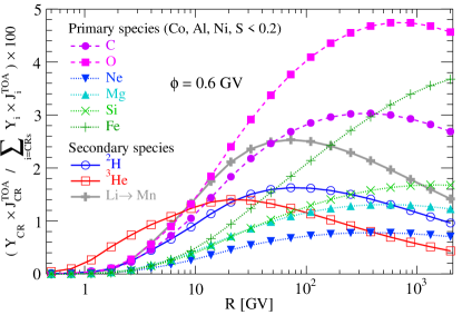
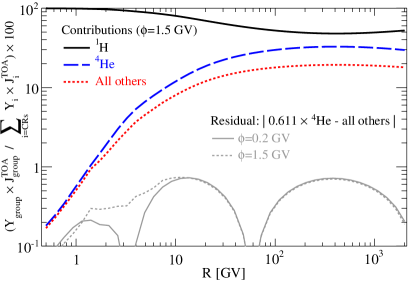
Figure 1: Fractional contribution w.r.t. the total (all species) as a function of rigidity, see Eq. (3.1). Top panel: zoom in on contributions larger than 0.2% for secondary species and for primary species heavier than He. Bottom panel: contributions from ¹H (solid black line), ⁴He (dashed blue line), and all others (dotted red line). To check whether accounting for the contribution of all other species as a scaling of ⁴He is a good approximation, the thin grey lines show their residual of the difference, i.e. $|0.611\times$⁴He - ‘all others’$|$ (solid and dashed lines correspond to minimal and maximal modulation periods).

Focusing on the fourth column (slope $C_{2}$), CRs fall in two groups with either $C_{2}\approx 2.8$, or $C_{2}\approx 3.0$. They correspond respectively to the so-called primary species (CRs accelerated in sources and propagated in the Galaxy) and secondaries species (spallative products of primary species). Furthermore, heavier species suffer more inelastic interactions than lighter ones during propagation, providing a flatter IS flux at low energy. The last two columns on Table 1 show that:

1. the contribution to count rates of heavy nuclei are significant up to Ni: low fluxes for heavy species are redeemed by the number of nucleons available in the yield function;

2. primary species contribute more than secondary ones: the contribution of heavier species $(Z\geq 3)$ w.r.t. to He, in this simple estimate, is $(Z\geq 3)/{\rm He}=0.480$, in agreement with the value 0.428 used in Usoskin et al. (2011);

3. secondary species $Z\geq 3$ contribute up to $\sim 4\%$ of the total, but due to a steeper slope w.r.t. primary species, their contribution decreases with rigidity;

4. the ²H and ³He isotopes also contribute to 4% of the total, and they should be dealt with separately from the rest because of their different A/Z value (they are not similarly modulated).

Anticipating on the description of a realistic yield function (presented in Sects. 4.2 and 4.3), Fig. 1 shows the result of the full calculation (without approximation) Eq. (3.1), as a function of rigidity (for TOA fluxes modulated at $\phi=600$ MV). The top panel zooms in on the fractional contributions of secondary species, and primary species heavier than He. The numbers are in fair agreement with those given in the last column of Table 1, but with two noteworthy features:

1. the contributions are not constant with energy, peaking between $10-50$ GV for secondary species, while constantly increasing for primary species. The heavier the species, the larger the increase. This is explained by the increase of the ratio of heavy to light primary species with energy, due to spallation effects at low energy (see Fig. 14 of Putze et al. 2011). As a result, at 100 GV, the Fe contribution is almost at the level of the C one;

2. ²H has a different A/Z ratio than all other species shown in the top panel, hence its contribution is shifted to lower rigidity.

The bottom panel of Fig. 1 shows the contributions of ¹H=H-²H (50%), ⁴He=He-³He (30%), and the sum of all other contributions (20%). The latter differs significantly from previous results:

1. the full calculation of the contribution of species heavier than helium gives

   $$s_{Z>2}=0.611^{+0.016}_{-0.009},$$ (6)

   instead of the value 0.428 obtained in the simple estimate and used in the literature;

2. we check that this approximation is better than 1% for all modulation levels, as illustrated by the difference between ‘true’ (all species) and ‘scaled ⁴He’ contributions, shown in grey. The uncertainty ${}^{+0.016}_{-0.009}$, i.e. $\sim 1.5-2.5\%$ on this factor, is obtained by propagating the errors on the CR IS flux parameters given in Table 1.

3.2 Degeneracy between $J_{\rm IS}$ and $\phi$

It has been shown that taking different parametrisations for the IS fluxes provides similar TOA fluxes and count rates, but with a shifted modulation parameters in time series (Usoskin et al., 2005; Herbst et al., 2010). Indeed, unless either strong assumptions are made on the transport coefficients in the solar cavity, or IS data are available, or sufficient data covering all modulation periods with a good precision exist, the degeneracy is difficult to lift.

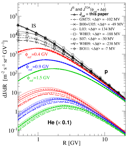
Figure 2: Proton (IS, symbols; TOA, lines) and He (TOA only) fluxes for different modulation levels, and different parametrisations of the IS fluxes found in the literature (see App. A): GM75 (Garcia-Munoz et al., 1975), B00+U05 (Burger et al., 2000; Usoskin et al., 2011), WH03 (Webber and Higbie, 2003), L03 (Langner et al., 2003), S07 (Shikaze et al., 2007), WH09 (Webber and Higbie, 2009), BO11 (O’Neill, 2010). The parameter $\langle\Delta\phi\rangle$ gives the mean modulation shift in order for $J^{\rm TOA}_{i}$ to best match $J^{\rm TOA}_{\rm ref}(\phi_{\rm ref})$, as illustrated for three reference modulation level $\phi_{\rm ref}=0.4$ GV (red), 0.9 GV (blue), and 1.5 GV (green). See text for discussion.

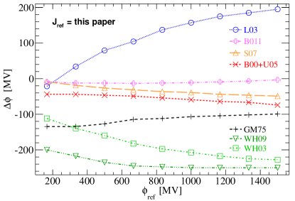
Figure 3: Value of the modulation shift $\Delta\phi_{i}$ to add to the reference modulation level $\phi_{\rm ref}$, for $J^{\rm TOA}_{i}(\phi_{\rm ref}+\Delta\phi_{i})$ to be as close as possible to $J^{\rm TOA}_{\rm ref}(\phi_{\rm ref})$. The index $i$ runs on the IS flux parametrisations shown in Fig. 2 (see also App. A).

To illustrate this point, Fig. 2 shows the IS proton flux (symbols) for several parametrisations behaving very differently at low energy. The reference IS flux (star) is the one fitted in the previous section. We then modulate protons for this reference flux (solid lines) at three different modulation levels ($\phi_{\rm ref}=0.4$ GV in red, 0.9 GV in blue, and 1.5 GV in green). Taking each IS flux parametrisation in turn, we search for the shift $\Delta\phi_{i}$ to apply to $\phi_{\rm ref}$ in order to minimise the difference between (i) the reference flux modulated at $\phi_{\rm ref}$ and (ii) a given IS parametrisation $i$ modulated at $\phi_{\rm ref}+\Delta\phi_{i}$. As can be seen on the figure, there always exists a value for which all the fluxes are very close to one another: this is what is meant by a degeneracy between the IS flux parametrisation and the modulation parameter value. The shift to apply slightly depends on $\phi_{\rm ref}$ itself (Fig. 3 in Herbst et al. 2010). It is illustrated in Fig. 3 showing $\Delta\phi_{i}(\phi_{\rm ref})$ for all IS flux parametrisations. Except for WH09 (Webber and Higbie, 2009), the most recent parametrisations are in better agreement than the older ones. The BO11 model (O’Neill, 2010) is the most compatible with the present study.

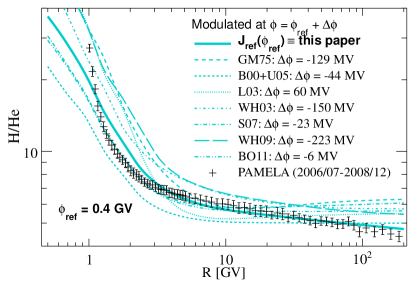
Figure 4: p/He ratio (vs rigidity) modulated at $\phi_{\rm ref}+\Delta\phi_{i}$ for all IS parametrisations $i$ shown in Fig. 2. The reference modulation level is taken to be $\phi_{\rm ref}=400$ MV for PAMELA data (’+’ symbols) taken from PAMELA Collaboration et al. (2011).

He fluxes ($\times 0.1$) are also shown in Fig. 2: the solid line is our best-fit IS flux, others He fluxes being obtained by scaling protons by 0.05 (Usoskin et al., 2005). For a better view, p/He ratios for all parametrisations are plotted in Fig. 4 (for $\phi_{\rm ref}=400$ MV), against the recent PAMELA data (PAMELA Collaboration et al., 2011). We find that the following scaling values give less scatter w.r.t. the data:

$$f_{{\rm He}/{\rm p}}\equiv\frac{dJ_{\rm He}/dR}{dJ_{\rm p}/dR}=\begin{cases}0.0525\quad\textrm{(GC75)},\\ 0.0475\quad\textrm{(B00+U05)},\\ 0.0550\quad\textrm{(L03)},\\ 0.0560\quad\textrm{(WH03)},\\ 0.0525\quad\textrm{(S07)},\\ 0.0605\quad\textrm{(WH09)}.\end{cases}$$ (7)

3.3 Dealing with IS flux uncertainties in count rate and $\phi$ time series

The above degeneracy prevents us from obtaining substantial constraints on the IS flux but not on count rate calculations.

TOA flux uncertainty

It can be estimated in two different approaches:

1. ‘data’ uncertainty: we assume that the reference IS flux model is the correct one, so that TOA uncertainties are directly obtained from the uncertainty on the fitted flux parameters (see Table 1). This gives a $\sim 2.5\%$ relative uncertainty, as shown in Fig. 5 for H (magenta dashed line) and He (red dotted line);

2. ‘model scatter’ uncertainty : lacking conclusive evidences to favour a particular IS flux shape, we can alternatively assume that all parametrisations $i$ are equally valid to provide similar (but not equal) effective TOA flux values. Plugging the appropriate effective modulation level $\phi_{\rm ref}+\Delta\phi_{i}$ to get, for each IS flux model $i$, its effective TOA flux (see Fig. 3), we form the quantity

   $$S_{i}(R)\equiv\frac{J_{i}^{\rm TOA}(\phi_{\rm ref}+\Delta\phi_{i})-J_{\rm ref}^{\rm TOA}(\phi_{\rm ref})}{J_{\rm ref}^{\rm TOA}(\phi_{\rm ref})}.$$

   The “model scatter” uncertainty is obtained by keeping minimal and maximal values of $S_{i}(R)$ over several $\phi_{\rm ref}$ and IS flux parametrisations $i$ (we discard L03 which is too far away from the data). In Fig. 5, the corresponding curves are shown for He (blue stars) and H (cyan circles). Note that some of the IS flux spectra used in this approach are probably already excluded by current data, so that the uncertainty range $\sim 10-30\%$ for H and He is (certainly too) conservative.

The uncertainty related to the contribution of heavier species should also be taken into account: the ‘scaling approximation’ factor Eq. (6) to account for CR heavier than He gives $s_{Z>2}=0.611\pm 2.5\%$.

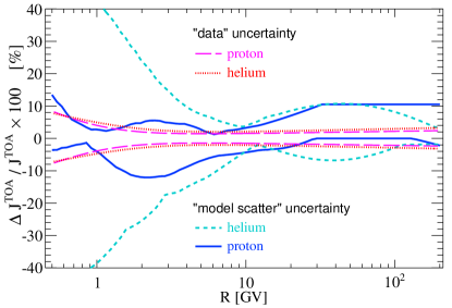
Figure 5: Relative uncertainty (envelopes) on the p and He TOA fluxes. The long-dashed pink and dotted red lines “data uncertainty” are calculated from the uncertainties on the fit on the CR p and He data (see Table 1). The solid blue and dashed cyan lines represent the ‘model’ dispersion (related the choice of the IS flux and modulation model). This uncertainty is propagated to calculated count rates in Sect. 5.2.1.

Impact on $\phi$ reconstruction

Our ignorance of the real IS flux shape has a strong impact on the determination of the modulation level $\phi$. However, it can be absorbed as a global (i.e., time-independent) shift $\Delta\phi$, once a given IS flux model is chosen. As seen from Fig. 3, the shift can be quite large (from -250 MV to 200 MV). To obtain times series (and their uncertainties) and compare different results given in the literature, the procedure is as follows: (i) calculate $N_{\rm ref}(t)$ and $\phi_{\rm ref}(t)$ from a reference $J^{\rm IS}_{{}^{1}\textrm{H}{},{\rm ref}}(R)$ and $(1+s_{Z>2})\times J^{\rm IS}_{{}^{4}\textrm{He}{},{\rm ref}}(R)$; (ii) the modulation level $\phi_{i}(t)$ for any given IS flux parametrisation $J^{\rm IS}_{i}$ is then simply related to the reference one:

$$\begin{cases}N^{\rm calc}(t)=N_{\rm ref}(t)\pm\Delta N_{\rm ref}^{\rm TOA}(t),\\ \phi_{i}(t)=\phi_{\rm ref}(t)\pm\Delta\phi_{\rm ref}^{\rm TOA}(t)+\Delta\phi_{i}^{\rm IS};\end{cases}$$ (8)

In the above equations, $\Delta N_{\rm ref}^{\rm TOA}$ and $\Delta\phi_{\rm ref}^{\rm TOA}$ are evaluated by propagating uncertainties of TOA flux quantities (see Fig. 5).

4 Atmospheric propagation, yield function, and detectors

When entering the Earth atmosphere, CRs initiate cascades of nuclear reactions involving primary energetic particles (mainly hydrogen and helium but also heavier nuclei) and atmospheric nuclei such as oxygen or nitrogen. The so-called Extensive Air Showers (EAS) generate secondary particles along their path, to be detected by ground-based instruments.

In this section, we discuss the generation of secondary particles (Sect. 4.1) as an input to provide a new yield function parametrisation (Sect. 4.2) for NMs (Sect. 4.3) and muon detectors (Sect. 4.4). We also discuss neutron spectrometers (Sect. 4.5) as a mean to study seasonal effects in NMs.

4.1 Atmospheric propagation of secondaries (n, p, $\mu$)

The secondary atmospheric radiation field is composed of various hadronic components (mostly neutrons, protons, and pions). Charged pions undergo leptonic decays producing positive and negative muons. Key quantities are

• $\dot{\varphi}_{k}(T_{k},\vec{r},t)$: spectral fluence rate (cm^-2 s^-1 MeV^-1) of the $k$-type secondary particle at kinetic energy $T_{k}$, coordinates $\vec{r}=(\varphi,\,\lambda,\,h)$, and time $t$;

• $\varphi_{ik}^{l}(h,\,T_{i}\!\rightarrow\!T_{k})$: spectral fluence (MeV^-1) of the $k$-type secondary induced at altitude $h$ by a $i$-type primary of kinetic energy $T_{i}$, and incidence within the zenith angle range $[\theta_{l},\,\theta_{l+1}]$.

Table 3: AtmoRad main features.

Parameter ​	Qty	​​​Bins	Range	Unit
Primary $i$​	H	18	$[0.1-251.2]$	GeV/n
	He
Secondary $k$​	n	70	$[10^{-3}-10^{11}]$	eV
	p, $\mu^{\pm}$	25	$[10^{6}-10^{11}]$
Incidence	$[\theta_{l},\theta_{l+1}]$​​​	3	$\displaystyle\left\{0,\,\frac{\pi}{6},\,\frac{\pi}{3},\,\frac{\pi}{2}\right\}$	rad
Altitude	h	36	$[0-30]$	km asl

Several works were dedicated to numerically estimate the spectral fluence rate $\dot{\varphi}_{k}$ during the solar activity cycle (e.g., Roesler et al. 1998; Roesler et al. 2002; Sato and Niita 2006; Nesterenok 2013). We rely here on the database of spectral fluence values $\varphi_{ik}^{l}$ presented in Cheminet et al. (2013c), in which Monte Carlo (MC) calculations were performed with GEANT4 (Geant4 Collaboration et al., 2003). For any coordinates $\vec{r}$ and solar modulation potential $\phi(t)$, the spectral fluence rate $\dot{\varphi}_{k}$ is obtained from $\varphi_{ik}^{l}$ read from the database as follows:

$$\!\!\!\!\!\!\!\!\dot{\varphi}_{k}(T_{k},\vec{r},t)\!=\!S_{T}\!\! \!\!\times\!\! \!\!\sum_{l=1}^{3}\Omega^{(\theta_{l},\theta_{l+1})}\;\;\sum_{i}^{\rm CRs}\;\;\sum_{T_{i}^{\textrm{cut-off}}}^{T_{i}^{\rm max}}\Delta T_{i}\;\;\;\;\;$$

$$\!\!\times\!\! \!\!J_{i}^{\text{TOA}}(T_{i},\phi(t))\times\varphi_{ik}^{l}(h,\,T_{i}\!\rightarrow\!T_{k}),$$

with $S_{T}=\pi\cdot(R_{E}+h_{\text{max}})^{2}$, $R_{E}=6,378.14$ km (Earth radius), and $h_{\text{max}}=85$ km (highest atmospheric altitude).

A C++ routine named AtmoRad (ATMOspheric RADiation) developed at ONERA implements the various ingredients entering Eq. (4.1). It handles both QGSP_BERT_HP and QGSP_BIC_HP reference users’ physics lists. Table 3 lists the quantities (primary and secondary species) and bins (energy and altitude range, incidence angles) used. The calculations were validated by extensive comparison with measurements, especially for the neutron component (Cheminet et al., 2013b). In the following we use QGSP_BERT_HP physic’s list. Figure 6 is an illustration of the neutron, proton, and muon spectral fluence rates obtained at sea level with a cut-off rigidity $R_{c}=0.8$ GV (similar to conditions at the Oulu NM station). The solid and dotted lines correspond to a period of minimum and maximum solar modulation potential $\phi(t)$ equal to 0.4 GV and 1.5 GV, respectively. Muons are the most numerous particles above a few hundreds of MeV, but the relative contribution of various secondaries to count rates in a detector depends on its efficiency to each species.

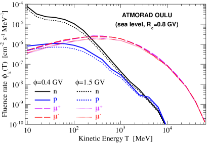
Figure 6: Illustration of secondary spectral fluence rates (see Eq. 4.1) calculated with AtmoRad (sea level, $R_{c}=0.8$ GV) for two solar modulation periods.

4.2 Yield function calculation and parametrisation

As given in Eq. (1), the yield function ${\cal Y}_{i}^{\cal D}(T_{i},h)$ of a ground-based detector ${\cal D}$ at altitude $h$ is its response (in count m² sr) to the unit intensity of primary CR $i$ at kinetic energy $T_{i}$. It can be described in terms of

• ${\cal Y}_{ik}^{\cal D}(T_{i},h)$: partial yield function from $i$-type primary species into $k$-type secondary species (in count m² sr);

• ${\cal E}_{k}^{\cal D}$: detector efficiency to $k$-type secondary species.

The yield and partial yield functions are then given by

$$\!\!\!\!\!\!{\cal Y}_{i}^{\cal D}(T_{i},h)\! \!=\! \!\sum_{k={\rm n,\,p,\,}\mu\dots}{\cal Y}_{ik}^{\cal D}(T_{i},h)\,,$$ (10)

$$\!\!\!\!\!\!\!\!\!{\cal Y}_{ik}^{\cal D}(T_{i},h)\! \!=\! \!S_{T}\!\sum_{l=1}^{3}\Omega^{(\theta_{l},\theta_{l+1})}$$

$$\!\times\! \!\int_{0}^{\infty}{\cal E}_{k}^{\cal D}(T_{k})\times\varphi_{ik}^{l}(h,\,T_{i}\!\rightarrow\!T_{k})dT_{k}.$$

Note that only the primary CR ions ¹H or ⁴He are evaluated below. For further usage, the resulting ${\cal Y}_{{}^{1}{\rm H}\rightarrow k}^{\cal D}$ and ${\cal Y}_{{}^{4}{\rm He}\rightarrow k}^{\cal D}$ are parametrised with a universal form ($T_{i/n}$ is the kinetic energy per nucleon of $i$)

$$\!\!\!\frac{{\cal Y}_{ik}^{\cal D}(T_{i},h)}{\exp(hf_{k})}\!=\!10^{\left(a_{ik}I-\frac{c_{ik}}{I^{d_{ik}}}-e_{ik}\right)}\,\,{\rm and}\,\;I\!\!=\!\log(T_{i/n})\!+\!b_{ik},\!\!\\$$ (12)

where the best-fit coefficients ($a_{ik}$, $b_{ik}$, $c_{ik}$, $d_{ik}$, $e_{ik}$, and $f_{k}$) are calculated for the various detectors ${\cal D}$ considered (the fit is appropriate for altitudes up to $h=5,000$ m). The yield function for any other primary of atomic mass $A$ at rigidity $R$ is rescaled from the ⁴He yield (at the same rigidity), namely

$${\cal Y}_{A}^{\cal D}(R,h)=\frac{A}{4}\times{\cal Y}_{{}^{4}{\rm He}}^{\cal D}(R,h)\,.$$ (13)

This assumption was tested with nitrogen, oxygen, and iron in Mishev and Velinov (2011), and was found to work well in the lower atmosphere (below 15 km).

4.3 Response and yield function for 6-NM64

Standardised neutron monitors (NM64 model) are widely used across the world to monitor CRs since the 1950s (Simpson, 2000). These detectors are especially powerful once integrated in a worlwide network (Bieber and Evenson, 1995; Dorman, 2004). They provide count rates with very interesting time intervals (typically one minute) thanks to the high efficiency of the detectors. An elementary unit of a 6-NM64 consists of six BF₃ proportional counter tubes which are mounted in raw and surrounded by a cylindrical polyethylene moderator. The tubes and the inner moderator are inserted in a large volume of lead (the producer). The outer walls of the NM64, the so-called reflector are again made of polyethylene or wood. A more detailed description of the standard NM64-type neutron monitors can be found elsewhere (Hatton and Carimichael, 1964).

NM response function

NMs are optimised to measure the high-energy hadronic component of ground level secondaries above 100 MeV (Simpson, 2000). However, in spite of their name, they are also sensitive to other secondary radiations (protons, pions, and muons). The efficiency of NM64 to various species have been calculated in the literature from MC simulations with FLUKA (Clem, 1999) or GEANT4 (Pioch et al., 2011). A detailed comparison of the efficiencies obtained in the literature is carried out in Clem and Dorman (2000) and Pioch et al. (2011): a very good agreement was found, be it for incident protons and neutrons (the calculation for the latter were also compared to the only existing beam calibration data from accelerator of Shibata et al. 1997, 1999). Differences up to a factor of two (above GeV energies) nevertheless exist depending on which of the GEANT4 physics model or event generator is selected. As our fluence is calculated with GEANT4, we choose to directly use the efficiency given in Pioch et al. (2011), also calculated with GEANT4, and which is in very good agreement with the results of Clem and Dorman (2000).

Relative contribution of secondary species ($n$, $p$, and $\mu$)

Table 4: Count rate fractional contribution from $k$ secondary particles at Oulu station (sea level and $R_{c}=0.8$ GV) during solar maximum and minimum periods, see Eqs. (14) and (15).

$\phi$ [GV]	$N^{\textrm{6-NM64}}$ [s-1]	$N_{k}/N$ [%]
		n	p	$\mu^{+}$	$\mu^{-}$
0.4	91	87.2	7.9	0.2	4.7
1.5	57	87.4	8.0	0.2	4.4

Although muons are the most numerous terrestrial particles (see Fig. 6), the efficiency of the 6-NM64 to muons is very low (3.5 order of magnitude below the hadrons at 1 GeV, see Fig. 5 of Clem and Dorman 2000). Hence they do not contribute much to the total count rate in a NM (Clem and Dorman, 2000). To back up this comment, we calculate the fraction of count rates from the secondary $k$ particles. Using Eqs. (4.1,10,4.2) in

$$N^{\textrm{NM}}({\vec{r}},t)=\sum_{k={\rm n,\,p,\,}\mu\dots}N^{\textrm{NM}}_{k}({\vec{r}},t),$$ (14)

the contribution $N^{\cal D}_{k}$ can be expressed to be

$$N^{\textrm{NM}}_{k}({\vec{r}},t)=\sum_{i={\rm CRs}}\int_{0}^{\infty}{\cal E}^{\textrm{NM}}_{k}(T_{k})\times\dot{\varphi}_{k}(T_{k},\vec{r},t)\;dT_{k}.$$ (15)

Folding the fluence rate (calculated with AtmoRad) with the 6-NM64 efficiency (from Clem and Dorman 2000), we gather in Table 4 the total count rate and the fraction due to the $k$-th particle, at Oulu location. Note that the total count rate calculated in the table is slightly lower than the observed one: this difference amounts to an extra normalisation of the yield function that will be addressed in our next study (see also Usoskin et al. 2011). The variation between a minimum and maximum modulation is almost a factor of two. The main contributions at sea level come from secondary neutrons (87%), protons (8%) and $\mu^{-}$ (5%), the $\mu^{+}$ contribution being negligible (0.2%). This fraction slightly changes for high altitude stations: the steeper increase of the number of nucleons relative to $\mu$ with altitude leads to a smaller muon fraction ($\sim 2.2\%$ at 2000 m and $\sim 1.2\%$ at 3500 m).

Results for our NM yield function

The partial yield functions ${\cal Y}^{\text{6-NM64}}_{ik}$ data points (symbols) calculated in this study from Eq. (4.2) are shown in Fig. 7 for different primary $i$ and secondary $k$ particles. Also shown are the best fits (lines) to these data relying on Eq. (12), whereas the best-fit parameters are gathered in Table 5. As already underlined above, the altitude dependence is steeper for nucleons than for muons. The energy dependence is similar to the yield function obtained in previous studies (see below), with a sharp cutoff at low energy, and a shallow power-law dependence at high energy.

Table 5: Best-fit parameters for a 6-NM64 yield function (in count m² sr) for a single tube with AtmoRad (see Fig. 7), relying on the parametrisation Eq. (12).

$\!\!i\!\rightarrow\!k\!\!$	$a_{ik}$	$b_{ik}$	$c_{ik}$	$d_{ik}$	$e_{ik}$	​​​$f_{k}$ [m-1]​​​
$\!\!\!\!p\!\rightarrow\!n\!\!$	-0.105​	2.862​	66.98​	2.648​	-5.432​	​​0.00067
$\!\!\!\!\alpha\!\rightarrow\!n\!\!$	-2.442​	5.484​	138.9​	0.834​	-48.71​
$\!\!\!\!p\!\rightarrow\!p\!\!$	0.5281​	1.588​	142.0​	6.295​	-1.367​	​​0.00069
$\!\!\!\!\alpha\!\rightarrow\!p\!\!$	0.2219​	1.803​	132.6​	4.753​	-3.219​
$\!\!p\!\rightarrow\!\mu^{-}\!\!\!\!$	0.722​	0.686​	4.104​	4.742​	-0.802​	​​0.00025
$\!\!\alpha\!\rightarrow\!\mu^{-}\!\!\!\!$	0.626​	1.276​	70.48​	5.824​	-1.340​

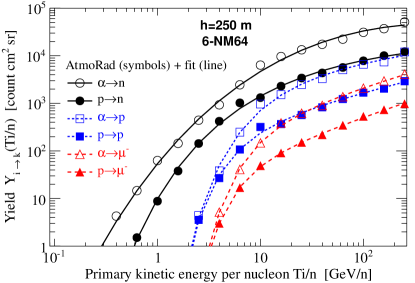
Figure 7: Levenberg-Marquardt fit of the AtmoRad yield function for secondary neutrons, protons, and negative muons at +250 m for a 6-NM64. The corresponding fit parameters are gathered in Table 4.

Comparison to other yield functions

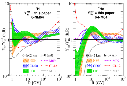
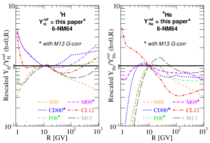
Figure 8: Ratio of various yield functions from the literature to ours (see App. B) for ¹H (left panels) and ⁴He (right panels): N89 (Nagashima et al., 1989, 1990), CD00 (Clem, 1999; Clem and Dorman, 2000), F08 (Flückiger et al., 2008), M09 (Matthiä 2009; Matthiä et al. 2009), CL12 (Caballero-Lopez and Moraal, 2012), M13 (Mishev et al., 2013). Top panel: lines are evaluated at sea level altitude, and filled areas show the dispersion of results related to a different altitude dependence in the different parametrisation (when available) for $h\in[0-2]$ km. Bottom panel: The yields are rescaled at 10 GV (so that the ratio is 1), and the geometrical factor correction proposed in Mishev et al. (2013) is applied to theoretical calculations (see Eq. 22 in App. B).

The total yield function ${\cal Y}^{\textrm{6-NM64}}_{i}$ (summed over all $k$ secondary particles) is compared to previous calculations in Fig. 8. The figure shows the ratio of any given parametrisation to ours at sea level (lines), for protons (left panels) and helium (right panels). For parametrisations provided with the altitude dependence (N89, CD00, F08, and ours), the shaded areas in the top panels show the dispersion w.r.t. the reference yield function altitude dependence, in the 0-2 km range. The different parametrisations rely on several MC generators/atmospheric models/NM responses (Clem, 1999; Flückiger et al., 2008; Matthiä et al., 2009; Mishev et al., 2013) or latitude and altitude surveys (Nagashima et al., 1989; Caballero-Lopez and Moraal, 2012). In that respect, the various yield functions can be considered to be in fair agreement. Because of the overall uncertainties in the modelling, the results are usually taken to be up to a global normalisation factor. This absorbs part of the difference if one is interested in count rate studies (e.g., Usoskin et al., 2011). The bottom panel shows the same quantity as in the top panel, but rescaled to 1 at 10 GV. Actually, Mishev et al. (2013) recently proposed a correction factor $G$ to account for a hitherto forgotten geometrical factor (related to the NM effective size). These authors find that this correction is necessary to match existing latitude NM surveys (see also Sect. 5.1.2). In principle, this correction (see Eq. 22) must be applied to any theoretical calculations, i.e. this work, CD00, F08, and M09 (it is by construction included in M13). These G-corrected yields at sea level altitude (renormalised at 10 GV) are shown in the bottom panel of Fig. 8: a quite good agreement is now found in the $5-50$ GeV range, where most of the counts come from (see below). This scatter (of the yield functions) is propagated to calculated count rate uncertainties in Sect. 5.2.1.

4.4 Cosmic-ray muon intensity

Table 6: Best-fit parameters for the yield function (in m² sr) of a generic $\mu$ detector with AtmoRad (see Fig. 9), relying on the parametrisation Eq. (12). Positive and negative muons are counted together.

$\!\!i\!\rightarrow\!\mu\!\!$	$a_{ik}$	$b_{ik}$	$c_{ik}$	$d_{ik}$	$e_{ik}$	​​​$f_{k}$ [m-1]​​​
$\!\!p\!\rightarrow\!\mu\!\!$	0.9116​	2.068​	664.1​	5.818​	2.755​	​​0.00025
$\!\!\alpha\!\rightarrow\!\mu\!\!$	-0.1315​	1.789​	49.75​	2.495​	-3.702​

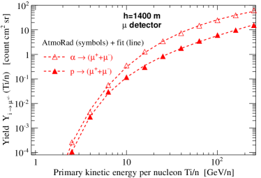
Figure 9: Levenberg-Marquardt fit of the AtmoRad yield function for muons at +1400 m (Auger altitude). The corresponding fit parameters are gathered in Table 6.

At sea level, muons are the most abundant charged particles, and they can be used in principle to monitor solar activity. Experimental aspects related to the detection of atmospheric muons are discussed, e.g., in Cecchini and Spurio (2012). Muon telescopes generally consist of layers of charged particle detectors and absorbing material, with the capability to determine the direction of $\mu$ arrival. The quantity of material crossed by the $\mu$ sets the detector threshold, which increases with the zenith angle for multi-directional telescopes. Some astroparticle physics detectors have also shown exquisite sensitivities to muons, as exemplified, on the one hand, by the measurements by L3 magnetic muon spectrometer at the LEP collider at CERN (L3 Collaboration et al., 2004), or on the other hand, by the huge array of surface detectors at the Pierre Auger Observatory (Pierre Auger Collaboration et al., 2011). In particular, The Pierre Auger Observatory, thanks to its 3,000 km² collection area, provides interesting data in the context of solar activity monitoring. The Auger scaler data (corrected for pressure), publicly available, are 15 minutes averages of the scaler rates, recorded since 2005. The threshold of the scaler mode is very low with a very high efficiency, so that in practice, it allows a muon counter equivalent mode (the scaler data variability were found to be well correlated with NM variations, Pierre Auger Collaboration et al. 2011).

In order to compare the behaviours of NMs and muon detectors, we calculate from AtmoRad the yield function of a perfect muon detector of 1 m². In AtmoRad, muons were validated by a cross-comparison with the expacs code, itself validated on CAPRICE 97 data (Kremer et al., 1999). The best-fit parameters relying on Eq. (12) are gathered in Table 6. This parametrisation should provide a fair estimate of the expected variability, e.g., for the Auger scaler data. Above 10 GV, we checked that it is in very good agreement with the results of Poirier and D’Andrea (2002) for protons. It is used in the rest of the paper to illustrate the results to expect from a generic muon detector.

4.5 Neutron spectrometers to study NM count rates

Recently, Bonner Sphere Spectrometers (BSS) were deployed at ground level and mountain altitudes in order to characterise the CR-induced neutron spectrum over long-term periods for dosimetry or microelectronics reliability purposes (Rühm et al. 2009a; Hubert et al. 2013). Unlike NMs, BSS are only sensitive to the neutron component. However, BSS are far less efficient than NMs and dynamics of one spectrum per hour can be reached at best (in high altitude stations). A BSS designed to cover a wide range of energies (from $10^{-2}$ meV to GeV) generally consists of a set of homogeneous polyethylene (PE) spheres with increasing diameters $d$. A high pressure ³He spherical proportional counter placed in the centre allows high detection efficiency. Additionally, spectrometers include some PE spheres with inner tungsten or lead shells in order to increase the response to neutrons above 20 MeV. These extended spheres (HE) behave like small NMs.

After an unfolding procedure (Cheminet et al., 2012b), the neutron spectral fluence rate $\dot{\varphi}_{n}^{\text{BSS}}(T_{n},\vec{r},t)$ can be derived from BSS data (i.e., count rates $M_{d}(\vec{r},t)$ for each of the $d$-Bonner sphere). The neutron component is very sensitive to local changes induced by meteorological and seasonal effects. BSS measurements allow to quantify such variations and to correlate them with variations expected/observed in NM count rates: we recall that neutrons amount to $\sim 87\%$ of the total count rate in NMs (see Table 4). Considering the local neutron count rate $N_{n}^{\textrm{X-NM64}}(\vec{r},t)$ of a $X$-NM64 at the BSS coordinates, we have

$$N_{n}^{\textrm{NM}}(\vec{r},t)=\frac{X}{6}\int_{0}^{\infty}{\cal E}_{n}^{\textrm{NM}}(T_{n})\,\,\dot{\varphi}_{n}^{\text{BSS}}(T_{n},\vec{r},t)\,\,dT_{n}.$$ (16)

BSS measurements are used to study the seasonal snow effects of NMs in Sect. 5.3.

5 Count rates: variations and uncertainties

In this section, count rates are calculated from Eq. (1), which involves the yield function ${\cal Y}^{\cal D}_{i}(h,R)$, the modulated fluxes $J^{\rm TOA}_{i}(t)$ for all CR species $i$, and the geomagnetic transmission ${\cal T}(R,\vec{r},t)$. To validate our code, we compare count rate variations (vs $R_{c}$) to existing latitude surveys (Sect. 5.1). We then propagate, on count rates, IS flux and yield function uncertainties (Sect. 5.2.1), and geomagnetic transmission function uncertainties (Sect. 5.2.2). We conclude the section with time dependent effects (on count rates) unrelated to solar modulation (Sect. 5.3).

Here, the altitude is set to $h=0$ m, but this value is not important. Indeed, although partial yield functions depend strongly on $h$ (see Table 5), the altitude and energy dependences are not coupled. This remains true for the total yield function (hence count rates) of $\mu$ detectors, and mostly true for NMs: the altitude dependence acts as a global factor that disappears when relative rate variations and relative errors are considered (as done below).

5.1 Count rate variation $N(R_{c},\,\phi)$ vs $R_{c}$

5.1.1 Relative contribution per rigidity bin

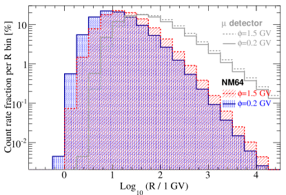
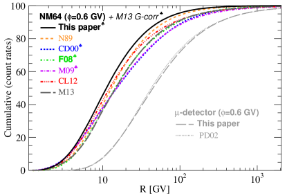
Figure 10: Origin of count rates for a polar response function (no rigidity cut-off). Top panel: relative contribution per rigidity bin at two modulation periods for NM64 detectors (blue and red shaded bars) and $\mu$-like detectors (thick solid and dashed grey lines). For instance, primary CRs between 10 and 20 GV contribute to 20% of the total counts in NMs, but only 10% in $\mu$ detectors. Bottom panel: cumulative of the count rates for several yield functions for NM64 (compared in Fig. 8, see also App. B) and $\mu$-detector (PD02 is the $\mu$ yield function from Poirier and D’Andrea 2002). NM64 yield functions indicated with a club^♣ ($G$-corr) are corrected for the $G$ factor of Mishev et al. (2013)—see text and Eq. (22) for details.

The top panel of Fig. 10 shows (considering the contribution of all CR species) for a polar response function (i.e. $R_{c}=0$) the fractional contribution per rigidity bin of the integrand ${\cal Y}\times J^{\rm TOA}$. The two shaded areas correspond to a period of minimal (blue shaded area) and maximal (red hatched area) modulation level. For CRs below 1 GV and above $\sim 50$ TV, the contribution is less than 1% of the total: this mitigates the impact of having large differences at low and high energy between various yield function parametrisations (see Fig. 8). The CR rigidity range contributing most to the count rates is shifted to higher energy when the modulation level is increased, or when sub-polar NM detectors ($R_{c}>0$) are considered.

The bottom panel of Fig. 10 proposes a complementary view, that is the cumulative of the count rates with $R$ (also for a polar response function). For MC-based yield function parametrisations (this paper, CD00, F08, M09), we take into account the $G$-correction of Mishev et al. (2013). All parametrisations give quite similar results, where 50%, (resp. 80% and 90%) of the count rates are reached when integrating up to 10 GV (resp. 30 and 70 GV). The value of the highest energy contributing is very sensitive to the high-energy slope of the yield function. For instance, we chose for CD00 and F08 (see App. B) a high energy extrapolation ${\cal Y}\propto E^{0.5}$. Would a ${\cal Y}\propto E$ chosen instead, 80% of the total count rate would be shifted from $R=30$ GV to 80 GV. It is thus important for future MC-based calculations to push the rigidity range up to 1 TV.

On both the top and bottom panels of Fig. 10, the result for a muon detector is shown in grey lines. The solid and dashed lines correspond respectively to periods of minimal and maximal modulation level. With respect to NMs, the mean energy contributing to count rates is shifted to higher energy, in a region where the impact of the solar modulation is smaller. Hence, the relative count rate variation $\Delta N/N$ to a change of the modulation level $\Delta\phi$ is smaller for $\mu$ detectors than for NMs.

5.1.2 Comparison to latitude survey data

Latitude survey experiments onboard planes, trucks, or ships cruising between equatorial and polar regions is another tool to derive yield functions and/or to compare with direct count rate calculations (Dorman, 2009). Monthly long ship surveys are generally performed during solar minimum periods—the most stable in terms of modulation changes—, in order to be only sensitive to rigidity cutoff effects (Moraal et al., 2000).

Data available

The solar cycle has an 11-year periodicity, and several surveys were carried out at minimum activity since the 50’s: 1954 (Rose et al., 1956; Keith et al., 1968), 1965 (Carmichael et al., 1965; Keith et al., 1968), 1976 (Potgieter et al., 1979; Stoker et al., 1980), 1986 (Moraal et al., 1989), 1997 (Iucci et al., 2000), but none that we are aware of in the last solar minimum period. The data from 1965 are discarded since they were found to differ from the similar 1954 and 1976 survey data (Potgieter et al., 1979). Data from 1976, 1986, and 1997, are also found to be in agreement (see, e.g., Fig. 4 of Mishev et al. 2013), with 1997 data thoroughly corrected from meteorological and geomagnetic effects (Iucci et al., 2000; Villoresi et al., 2000; Dorman et al., 2000).

Table 7: NM latitude surveys and corresponding CR data available at the same epoch.

Survey date	Ref.	CR data	Exp.	Ref.
12/75-11/76	[Pot79]	07/77	Balloon	[Web83]
		10-11/77	Voyager1
05/86-10/87	[Mor89]​​	01-12/87	Voyager2†	[Seo94]
12/96-03/97	[Iuc00]	07/97	BESS 97	[Shi07]
2006-08	-	​​​​​​​07/06-12/08‡	PAMELA​​	[PAM11]​​​

^† $\phi$ estimated (from data at 23 AU) to be 500 MV (Seo et al., 1994).
^‡ Representative of 1986/1987 (Caballero-Lopez and Moraal, 2012).

To compare these data with calculations based on CR fluxes and yield functions, the knowledge of the modulation level to apply is critical. With no CR data available in 1954, we have to base our calculation on 1976, 1986, and 1997 CR measurements. We list in Table 7 the epoch of these surveys and the closest (in time) CR data available (retrieved from crdb).

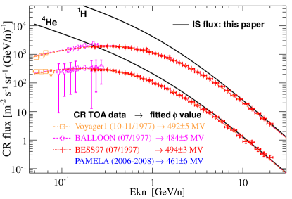
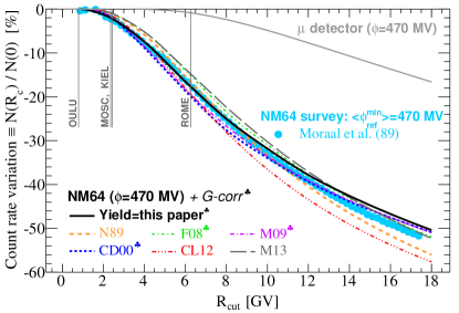
Figure 11: Top panel: CR data at epochs of NM latitude surveys (see Table 7), and best-fitted $\phi$ values (and corresponding TOA fluxes). Bottom panel: Count rate relative variation $N(R_{c})/N(0)$ for NM64 (various parametrisations, see App. B) and $\mu$-like detectors vs $R_{c}$. Yield functions indicated with a club^♣ ($G$-corr) are corrected for the $G$ factor Eq. (22) of Mishev et al. (2013). Circles are data from NM latitude survey data (Moraal et al., 1989). Vertical segments show the rigidity cut-off for a sample of NMs.

Modulation level at solar minimum

The CR data listed in Table 7 allow us to determine consistently (i.e., given our IS flux parametrisation) the modulation level $<\phi_{\rm ref}^{\rm min}>$. This level applies for epochs of minimal modulation. Figure 11 shows the bets-fit $\phi$ required to match CR TOA fluxes. A simultaneous fit of H and He data is performed using the force-field approximation (Sect. 2.2) and our reference IS flux parametrisation—Eq. (3) and Table 1—. Note that the value of $\phi$ for PAMELA is directly reproduced from Table 2. We find that all $\phi$ values are consistent with one another, and we take in the following $<\phi_{\rm ref}^{\rm min}>=470\pm 20$ MV. This value is slightly higher than the one used in Mishev et al. (2013).

NM and $\mu$-detector latitude dependence

Figure 11 shows, as a function of $R_{c}$, a comparison of the normalised (at $R_{c}=0$ GV) count rate variations (for various yield functions) to survey data (only the 1986-1987 survey is shown for clarity). The solar modulation level is set to $\phi=470$ MV, appropriate for a period of minimal activity (see above). We find, in agreement with the conclusions of Mishev et al. (2013), that taking into account the $G$-correction factor (see Eq. 22) gives a much better match to latitude survey data (the curves without this correction are not shown). NM-survey based yield functions (N89 and CL12) give a similar albeit slightly less good match. Note that the scatter observed from the use of the various yield functions is larger than the variation obtained by shifting the modulation $\phi_{\rm ref}^{\rm min}$ by $\pm 20$ MV.

Concerning the variation of count rates with $R_{c}$, as already underlined, count rates decrease when $R_{c}$ increase—$R_{c}$ is the lower boundary of the integral Eq. (1). Over the whole $R_{c}$ range, the variation is less marked for a $\mu$-like detector ($\lesssim 20\%$, grey line) than for NMs ($\lesssim 50\%$). This is understood as the mean rigidity of CRs contributing to the count rate is higher for the latter than for the former (see bottom panel of Fig. 10).

5.2 Count rate relative uncertainty $\frac{\Delta N}{N}(R_{c},\,\phi)$

For an overview of the various sources of uncertainties involved in count rate calculations, we refer the reader to the reference textbooks of Dorman (2004) for meteorological effects, and Dorman (2009) for cut-off rigidity effects.

5.2.1 Error from IS flux and yield function modelling

The two panels in Fig. 12 show the errors on the count rate calculation as a function of $R_{c}$ (for NM64 and $\mu$ detectors) propagated from the uncertainties on CR fluxes (top) and yield functions (bottom). For simplicity, the errors are symmetrised, i.e. we consider $({\rm err}_{\rm min}+{\rm err}_{\rm max})/2$.

For NM64 detectors, the solid blue line (resp. dashed red line) corresponds to the propagation of errors on the IS flux ‘data’ (resp. ‘model’) as discussed in Sect. 3.3 and shown in Fig. 5. These uncertainties are, to a very good approximation, independent of the solar modulation level and of the rigidity cut-off. It means that they contribute only to a global shift in count rate times series (no time dependence, and no detector location dependence). This uncertainty is at the level of $2-6$% for NMs, with a slightly larger range $2-8$% for $\mu$ detectors (dashed grey line). Future CR data (e.g. AMS-02) will likely shrink these uncertainties at the percent level.

On the same figure, the lines with symbols show the uncertainty related to the existing dispersion among the proposed NM64 yield functions in the literature (see Sect. 4.3, Fig. 8, and App. B). We recall that yield functions are generally considered up to a normalisation. To get a meaningful result, we re-normalised all count rates to a reference value (set arbitrarily to $R_{c}=6.3$ GV), leading to a pinch in the curves. There is a mild dependence on the modulation level, but the overall uncertainty is estimated to be below 8% over the whole $R_{c}$ range, and more particularly, at the $2-5$% level for NMs located at $R_{c}<10$ GV. The dispersion is much smaller for $\mu$ detector ($<0.2\%$, grey lines and symbols): the latter is probably not conservative and may reflect the fact the only two parametrisations of their yield function are used for this study.

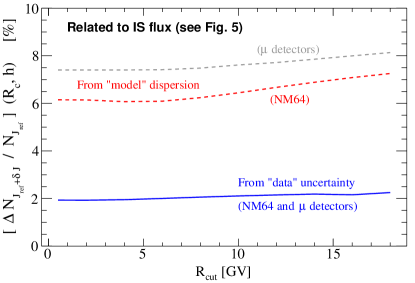
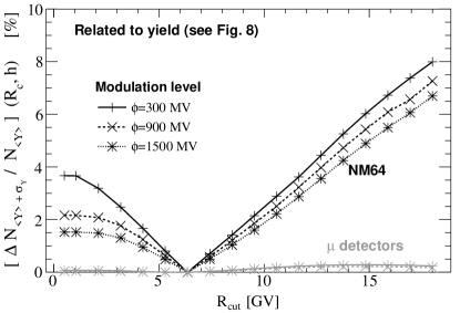
Figure 12: Relative uncertainty on count rates for NM64 and $\mu$ detectors. Top panel: uncertainty propagated from IS flux uncertainties. Bottom panel: uncertainty propagated from yield function dispersion (for NM64 in black symbols, $\mu$ in grey symbols). Note that the pinch observed is related to the arbitrariness in the choice of a reference $R_{c}$ to compare NM64 yield functions with one another.

5.2.2 Uncertainties from transmission function ${\cal T}$

A key parameter for calculations is the transmission function of charged particles in the geomagnetic field (Dorman, 2009). Several factors can be taken into account to have an estimate of the associated uncertainties on the count rates. Indeed, the transmission depends on the geographical longitude and latitude $(\varphi,\lambda)$, which can be calculated for a given state of the Earth magnetosphere (Smart et al., 2000). The latter varies in time, and its full description requires both the long-term evolution of the geomagnetic field (International Geomagnetic Reference Field) and the short-term magnetospheric field model (Tsyganenko and Sitnov, 2005; Kubyshkina et al., 2009; Tsyganenko, 2013). A good summary of the past studies and findings is given in Smart and Shea (2003, 2009).

The complicated structure of the geomagnetic field leads to a quasi-random structure of allowed and forbidden orbits, denoted ‘penumbra’. The effective vertical rigidity cut-off (see Cooke et al. 1991), used so far in this analysis ($R_{c}^{\rm eff}\equiv R_{c}$), consists in a weighted average value accounting for the allowed bands (between the upper and lower cut-off values). With the assumption that all regions contribute the same (flat spectrum hypothesis), it is given by (Dorman et al., 2008):

$$R_{c}^{\rm eff}\approx R_{\rm upper}-\sum_{i=R_{\rm lower}}^{R_{\rm upper}}\Delta R_{i}^{\rm allowed}.$$ (17)

In this approach, it follows that the transmission function is described by the step function $H(R-R_{c}^{\rm eff})$.

Short and long time variation of $R_{c}$

At each geomagnetic position and time $t$, an effective vertical cutoff rigidity $R_{c}$ can be calculated. For long term evolution, calculations with a fine position grid have been carried out at different epochs (e.g., Smart and Shea, 2008a, b). Over a 50 year (resp. 2000 year) evolution, increases or decreases of $R_{c}$ at the level of $\sim 5-10\%$ (resp. 30%) are expected (Shea and Smart, 2001; Flückiger et al., 2003; Masías-Meza et al., 2012; Herbst et al., 2013).

Short-term changes are more challenging computationally (Smart et al., 2003, 2006; Bütikofer et al., 2008): small time step calculations are required and an evolving magnetospheric model must be considered. On short timescales, an enhanced geomagnetic activity leads to a temporary change of the effective vertical rigidity cutoff (Flückiger et al., 1983, 1986; Kudela et al., 2008; Masías-Meza et al., 2012). In particular, during geomagnetic storms, decreases of $R_{c}$ by a few GV for several hours are predicted, and confirmed from NM data (Desorgher et al., 2009; Tyasto et al., 2013).

The impact of changing $R_{c}$ to $R_{c}+\delta R_{c}$ is shown in the top panel of Fig. 13. Whenever $R_{c}$ is increased, the count rates decrease, with a milder impact at epochs of high solar activity than for low activity. This is related to the steepness of the decrease of the count rate with $R_{c}$ shown in Fig. 11. For detectors located at $R_{c}<10$ GV, count rates over 50 years vary at most by -4% for NM64 (blue dashed lines), and -1% for $\mu$ detectors (dashed grey lines).

Allowed and forbidden rigidity: penumbra

A better description of the transmission function is the use of a sigmoid function, as done in the context of NMs (Kudela et al., 2008), or the CR experiments HEAO-3 (Ferrando et al., 1988) and AMS-01 (Bobik et al., 2006, 2009). The step function $H(R-R_{c}^{\rm eff})$ is the limit of a sigmoid of zero width. To see how good is this zero-width approximation, we compare count rates calculated with it and with the following sigmoid shape (centred on $R_{c}$):

$${\cal T}(R)=\frac{1}{2}\left[1+{\rm erf}\left(\frac{R-R_{c}}{\sqrt{2}\;\Delta R}\right)\right].$$ (18)

It is useful to define the width $\sigma$ of the sigmoid function to be

$$\sigma\equiv\frac{\Delta R}{R_{c}}.$$

A typical range of values reproducing best AMS-01 data (depending on the position) is $\sigma\sim 0.1-0.2$ for $R_{c}\gtrsim 2$ GV, and $\sigma\sim 0.1-0.5$ for $R_{c}<2$ GV.

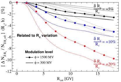
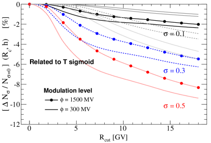
Figure 13: Relative uncertainty on count rates for NM64 and $\mu$ detectors (light grey curves) as a function of $R_{c}$, for two extreme values of the modulation level (lines, $\phi=300$ MV; symbols, $\phi=1500$ MV). Top panel: count rate change when moving from $R_{c}$ to $R_{c}+\delta R_{c}$. Bottom panel: count rate change from the use of a sigmoid Eq. (18) instead of a step function.

The bottom panel of Fig. 13 shows the ratio of count rates calculated for various values of $\sigma$ to count rates in the step function approximation. The sigmoid case gives less count rates than the step function case, an effect that increases with $R_{c}$ and with the width of the sigmoid. Moreover, the larger the modulation level $\phi$ (chained lines compared to lines), the smaller the effect. These behaviours are well understood if one keeps in mind how the contribution per rigidity band (described in Fig. 10) varies: compared to the step function, the sigmoid allows less contributions above $R_{c}$ (where it matters most), and more contributions below $R_{c}$. For mild values of $\sigma=0.3$, the change below $R_{c}=10$ GV (where most stations lie) is -4% at most for NM64 (blue dashed lines), and -2% for $\mu$ detectors (dashed grey lines).

Obliquely incident particles: apparent cut-off rigidity

With the advance of more powerful computers, obliquely incident CRs—and the ensuing secondary particles reaching the detector—could be considered (Rao et al., 1963; Clem et al., 1997; Dorman et al., 2008). Instead of weighting each vertical direction of the penumbra similarly as in Eq. (17), the vertical and non-vertical incident CRs are weighted according to the zenith angle dependent rigidity cutoff (assuming at first order that there is no azimuth dependence). This defines a so-called apparent vertical cut-off rigidity $R^{\rm app}_{c}$:

$$\!\!\!\!R^{\rm app}_{c}(R_{c})\equiv\frac{\int_{0}^{2\pi}d\phi\,\int_{0}^{\pi/2}\,\,R_{c}(\theta,\,\phi)\times{\cal Y}(R_{c},\,\theta,\,\phi)\,\,d\theta}{\int_{0}^{2\pi}d\phi\,\int_{0}^{\pi/2}\,\,{\cal Y}(R_{c},\,\theta,\,\phi)\,\,d\theta}.$$ (19)

Its calculation is more demanding than that for $R_{c}^{\rm eff}$, though approximations to speed up the calculation exist (Bieber et al., 1997). In terms of the apparent cut-off rigidity, Eq. (1) for count rates becomes

$$\!\!N^{\cal D}({\vec{r}})\! = \!\!\!\int_{\rm sky}\!\!\!\!\!d\Omega\int_{R_{c}(\Omega)}^{\infty}{\cal Y}^{\cal D}_{i}(R,h,\Omega)\,J(R)\;dR$$ (20)

$$= \!\!\!\int_{\rm sky}\!\!\!\!\!d\Omega\int_{R_{c}^{\rm app}}^{\infty}{\cal Y}^{\cal D}_{i}(R,h,\Omega)\,J(R)\;dR.$$

All our previous calculations still apply, replacing the vertical effective rigidity cut-off $R_{c}$ by the apparent rigidity cut-off $R^{\rm app}_{c}$ values.

Folding an NM64 yield function (calculated with FLUKA and HEAVY packages) with rigidity cut-off maps, Clem et al. (1997) found $R_{c}^{\rm app}>R_{c}$. The difference is $\sim 10\%$ for $R_{c}\approx 0.1$ GV, then it decreases and stay at $\sim 3\%$ above $R_{c}\gtrsim 8$ GV (see their fig. 11). Further investigations by Dorman et al. (2000, 2008) rely on a parametrised angular distribution of the yield function compared with NM survey data. We fit their Fig. 5 and obtain

$$\left(\frac{R_{c}^{\rm app}\!-\!R_{c}}{R_{c}}\right)\!\times\!100\!=\!\begin{cases}\!\frac{1.8}{R_{c}}\!-\!1.7\!+\!0.47R_{c}&\!\!\!{\rm if~{}}R_{c}>1,\\ 0&\!\!\!{\rm otherwise}.\end{cases}$$ (21)

Dorman et al. (2008) results go in the same direction as Clem et al. (1997) ones, though the $R_{c}$ dependence of the relative error is slightly different. The maximum shift of $R_{c}$ to $R_{c}^{\rm app}$ is $\sim 6\%$ for $R_{c}=18$ GV, and the shift decreases with decreasing $R_{c}$. The impact of this change on the count rate calculations can be directly read off the top panel of Fig. 13.

We underline that the effects related to the geomagnetic field are quite complex, and may be not all accounted for, as possibly illustrated by the not yet understood long-term decline of South pole neutron rates (Bieber et al., 2007, 2013).

5.3 Seasonal effects: pressure, temperature, snow coverage and water vapour

NM or muon detector count rates can be affected in many ways by meteorological and seasonal effects (Dorman, 2004). The quantities considered in this study are atmospheric pressure, temperature, the water vapour, and the snow coverage. For the latter, which is usually not included in public NM data, a comparison with the results of neutron spectrometers is used to assess the strength of the effect.

5.3.1 Atmospheric pressure

Atmospheric pressure effects are discussed in, e.g., Hatton and Griffiths (1968). Given $N_{0}$ particles observed at a reference atmospheric pressure $p_{0}$, their number $N$ at pressure $p$ is $N\approx N_{0}\exp\left[-\beta(p-p_{0})\right]$ (Dorman, 1974). The quantity $\beta$ is the barometric coefficient, which is obtained correlating secondary CR intensities and data for the atmospheric pressure. As illustrated in Paschalis et al. (2013), $\beta\sim 0.72\%$ hPa^-1 for the Athen NM station. Considering a typical 20 hPa variation translates into a $\sim 13\%$ count rate variation. The barometric coefficient strongly depends on the station location and on the considered detector Dorman (2004). Publicly distributed data are generally corrected for this effect. However, uncertainties on the barometric coefficients $\Delta\beta\sim 0.02$% hPa^-1 (Chilingarian and Karapetyan, 2011) lead to corrected data with count rate uncertainties $\Delta N/N|_{\text{Pressure}}\sim 0.2\%$.

5.3.2 Atmospheric temperature

The well-known temperature effect is detailed, e.g., in Iucci et al. (2000). For NMs, it amounts to -0.03%/^∘C, that is an Antarctica-to-equator temperature effect $\sim 1\%$, which is also the order of magnitude of the seasonal effect $\Delta N/N|_{\text{Temperature}}\sim 1\%$.

For muons, the temperature effect, which is dominant over all other effects, is discussed, e.g., in Dmitrieva et al. (2011). The seasonal effect is $\sim 8\%$ with smaller variation of $1-2$% on the background of seasonal trend, with a small dependence on $R_{c}$ (Clem and Dorman, 2000). It should be pointed out that this effect strongly depends on the zenith angle of incident muons. For $\mu$ data, real time correction for this effect is discussed in Berkova et al. (2011, 2012).

5.3.3 Water vapour

As discussed in Bercovitch and Robertson (1965) and in Chasson et al. (1966), an increase of atmospheric water vapour content attenuates the intensity of secondaries seen by a NM. To take into account this effect, they proposed a correction of the barometric coefficient $\beta$. The variation $\Delta\beta$ is estimated between -0.09% hPa^-1 and -0.15% hPa^-1, leading to a seasonal effect $\Delta N/N|_{\text{Water Vapour}}\sim 0.2-0.3\%$. Recently and for the first time, this effect was investigated (Rosolem et al., 2013) in a detailed simulation based on the neutron transport code Monte Carlo (MCNPX). In agreement with Bercovitch and Robertson (1965), the sensitivity of fast neutrons to water vapour effect was found to reach $\sim 10\%$ for sites with a strong seasonality in atmospheric water vapour, with a larger decrease of count rates in moist air than in dry air.

For muon detectors, pressure effects are also considered with barometric factor $\beta_{\mu}$, but lower than NM ones ($\beta_{\mu}=0.03\%$ hPa^-1).

5.3.4 Snow effect

The last effect discussed is the impact of snow on the neutron component (no effect is expected for the other secondary components). Recent works have shown that heavy snow fall impact strongly the 1 meV to 20 MeV neutron spectrum (i.e. thermal, epithermal and evaporation domains), while the cascade region ($>$ 20 MeV) is less affected (Rühm et al., 2012; Cheminet et al., 2013b). As a matter of fact, hydrogen in water molecule is responsible for enhanced thermalisation and neutron absorptions. In the context of NMs, the snow both in the surroundings and above NM shelters affect count rates.

Table 8: Main characteristics of stations running BSS for continuous measurements at ground level (upper half). The next to last rows give the NM count rates (from neutrons) calculated from BSS measurement using Eq. (16) in winter ($N_{n}^{\rm min}$) and summer ($N_{n}^{\rm max}$). The last two rows give an estimate for the snow seasonal effect for NM64.

Institute	hmgu		irsn/onera
Location	Zugspitze	Spitsbergen	Pic du Midi
h (m)	+2,650	0	+2,885
$R_{c}$ (GV)	4.0	0.0	5.6
Date	2004	6/07	5/11
Spheres PE	14	2	10
Spheres HE	14	2	2
$N_{n}^{\rm max}$ (s-1)	501.9	77.5	400.3
$N_{n}^{\rm min}$ (s-1)	470.3	75.8	364.6
$\frac{\Delta N_{n}}{N_{n}}$ (%)	-6.3	-2.2	-8.9
$\frac{\Delta N}{N}|_{\rm Snow}$ (%)	-5.3	-1.8	-7.6

BSS location and data

Data from three BSS are gathered to study the snow effect of the neutron component in NMs count rates. Two of them are run by the Helmholtz Zentrum München (HMGU) at mountain altitude at the summit of the Zugspitze in the German Alps, as described in Rühm et al. (2009a, b) and Rühm et al. (2012). The last one is operated by the French Aerospace Lab. (ONERA) at the summit of the Pic du Midi de BigorreCheminet et al. 2012a, b; Cheminet et al. 2013a, c). The main features of each experiment are highlighted in the upper half of Table 8.

As an illustration, Fig. 14 shows typical spectra obtained for the three above-mentioned BSS in summer and winter. The decrease of intensity for low and intermediate energies is clearly visible in winter, when heavy snow falls occur in the northern hemisphere.

NM64 seasonal effect from BSS data

As explained in Sect. 4.5, it is possible to derive the count rates $N_{n}$ due to neutron in NMs thanks to Eq. (16). We first show in Fig. 15, for the Pic du Midi case, the product of the NM64 response and the neutron spectra as a function of kinetic energy $E_{n}$. Although the majority of counts are due to cascade neutrons (above 20 MeV), evaporation neutrons are non negligible, and for both energy regions, the difference between summer and winter is significant.

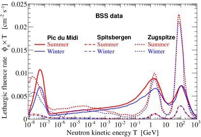
Figure 14: Neutron spectra obtained from BSS measurements at various locations. Data from Pic du midi are taken from Cheminet et al. (2013b), and from Rühm et al. (2012) for the other stations.

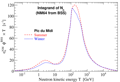
Figure 15: Integrand of Eq. (16) for the Pic du Midi case in summer and winter. The area under this function gives directly the expected count rates in NMs for the two seasons.

For NM64, the value of the count rate variations $\Delta N/N|_{\text{Snow}}$ due to seasonal effect are calculated taking into account the fact that neutrons constitute 87% of the total NM count rate. The results for the three stations are gathered in the lower half of Table 8: the effect varies between -1.8% and -7.6%. These estimations are consistent with data provided by, e.g., Tanskanen (1968) and Korotkov et al. (2011), with a variation about -5% recorded at NM station of Oulu, and -7% in Rome. They are also in agreement with the results of Rühm et al. (2012) based on Zugspitze and Spitsbergen data.

This confirms that snow has a significant and seasonal impact on NM count rates in stations that might know intense snow fall episodes (particularly at mountain altitudes). Indeed, recent effort are directed into having real-time and automated corrections for the snow effect in NM64 data (Korotkov et al., 2011, 2013). After this correction, these authors estimate a residual error of $\sim 0.4\%$.

5.4 Other effects

NM count rates depend on the detector surroundings and the atmosphere state, but they also depend on the reliability and stability of the equipment. To improve further the usefulness of the NM network, inter-calibration of all stations is required. Portable calibration NMs were discussed in Moraal et al. (2001), built soon after (Moraal et al., 2003), and several tests and validation carried out (Krüger and Moraal, 2005, 2010, 2011; Krüger et al., 2008; Krüger and Moraal, 2013). Note that the target goal for the calibrator was to reach an accuracy of $\leq 0.2\%$ (for spectral studies), which succeeded, as reported in Krüger and Moraal (2010). However, during the tests, several effects were measured, that are of importance and amount somehow to uncertainties.

First, the instrumental temperature effect (not related to the atmospheric temperature effect) was recently reconsidered by Krüger et al. (2008), who measured a $\sim 0.05\%/^{\circ}$ C change for NM64. However, this should not impact count rates as long as the detectors are kept in a small temperature range. More worrisome is the fact that different local conditions lead to an unpredictable spread of $\sim 4\%$ (Krüger and Moraal, 2010). Then the exact geometry of the detector (Hatton and Carimichael, 1964), whether it contains $n$ or $m$ tubes also slightly changes the efficiency of the detector (and in fine the yield function and count rates at various latitude): effects up to a few percent can exist (Hatton and Carimichael, 1964; Krüger et al., 2003), and in particular, differences up to $4\%$ were observed between the calibrator and a 3-NM64 (Krüger and Moraal, 2013). The last two issues may explain the need of detrending NM data in order to reach a coherent picture of solar activity for the various stations (Oh et al., 2013).

Finally, anisotropy effects (e.g., diurnal and semi-diurnal variations) also exist, but are beyond the scope of this paper. Their amplitudes depend on many parameters (species measured, location of the detector, etc.), which complicates the study of ground-level events. We refer the interested reader to Dorman (2004).

6 Conclusions: count rate variation and uncertainty iso-contours in the $(R_{c},\,\phi)$ plane

We have made a detailed study of count rates (and uncertainties) for neutron monitors and $\mu$ detectors, as a function of the rigidity cut-off and the modulation level $\phi$, in the context of the force-field approximation.

6.1 Input parameters

First, we have re-assessed (and compared with previous results from the literature) two key ingredients entering the calculation, namely IS fluxes and yield functions.

1. Results for IS fluxes:

   • we propose a new set of IS flux parametrisations for elements $Z=1-28$, see Eq. (3) and Table 1;

   • we improve the calculation of the factor accounting for heavy species ($Z\geq 3$) as an extra contribution of ⁴He (for NM and $\mu$ detector count rate calculations). The required extra amount of ⁴He is found to be $0.611^{+0.016}_{-0.009}$ ⁴He (to be compared with 0.480 used in previous studies). We check that making the substitution is accurate at better than the percent level over the whole rigidity range;

   • as previously studied in Herbst et al. (2010), it is always possible to recover the same TOA fluxes, starting with different combinations of IS fluxes and solar modulation parameter $\phi$ (degeneracy between $\phi$ and the IS flux). Equation (8), to be used with Fig. 3, provides a simple recipe to move from one $\phi$ time series to another, depending on the choice of the IS flux (all formulae are gathered in app. A);

   • we evaluate the uncertainty on TOA ¹H and ⁴He fluxes (see Fig. 5), directly from the fit (of our reference flux) to the data and their errors, or from the dispersion of TOA fluxes obtained with the use of several parametrisations of the IS flux (modulated at their appropriate value, as underlined above). We arrived at a 5% uncertainty for the former, and a probably overestimated $\sim 10-20\%$ dispersion (energy dependent) for the latter.

2. Results for the yield functions:

   • we propose a new yield function parametrisation Eq. (13) for primary CR protons and heliums, evaluated for NM64 in Table 5 and for $\mu$ detectors in Table 6;

   • we provide a systematic comparison of available yield functions in the literature (see Fig. 8, all formulae are gathered in App. B). Differences of a factor of a few exist around a few tens of GV, these differences increasing at lower and higher rigidity. A better agreement at high energy is obtained when accounting for the geometrical correction factor of Mishev et al. (2013);

   • after renormalisation to a reference rigidity, the dispersion for the various yield functions can be used to estimate the uncertainty on count rates (see below).

6.2 Count rates and uncertainties

Using these inputs, we have been able to characterise the count rate dependence on several parameters and related uncertainties.

• for polar stations, 90% of the count rates are initiated by CRs above 5 GV for NM64 and above 10 GV for $\mu$ detectors (see Fig. 10);

• we validate NM64 yield functions against latitude surveys in two steps:

  1. we derive the solar modulation level (from CR data, based on our reference IS flux) at the time of these surveys (minimum activity)—see top panel of Fig. 11. We find $\phi_{\rm min}\approx 470$ MV, a value slightly higher but in agreement with the value used in other works using these same surveys.

  2. a comparison of various yield functions from the literature confirms that the geometrical correction factor proposed in Mishev et al. (2013) is mandatory to better fit NM survey data. This effect and the energy dependence of MC yield function calculations in the 100 GV$-$1 TV should be further explored. When this correction is applied to all MC-based yield function (as opposed to yield functions derived from NM data surveys), a consistent picture emerges, with all modelling in fair agreement with one another. Rather unexpectedly, a slightly better fit to all the survey data (up to a rigidity cut-off of 10 GV) is given by the new yield function we propose.

• We propagate the uncertainties obtained for the IS flux and yield function to the calculated count rates:

  1. a $\phi$ and $R_{c}$ independent uncertainty of 2% (resp. $6-8\%$) is related to IS flux from data uncertainty (resp. from IS flux model dispersion), see top panel of Fig. 12. The scaling factor (for $Z>2$ species) uncertainty leads to another $0.6\%$. This applies to NM64 as well as to $\mu$ detectors;

  2. an $R_{c}$ dependent (and slightly dependent on $\phi$) uncertainty smaller than $2-4\%$ for $R_{c}<10$ GV (resp. $6-8\%$ for $R_{c}<18$ GV) is related to NM64 yield function dispersion, see bottom panel of Fig. 12. This uncertainty is smaller than 0.2% for a $\mu$ detector.

• We revisit the uncertainties related to the transmission function of CRs in the geomagnetic field. Focusing on effective vertical rigidity cut-off below $R_{c}=10$ GV (where most stations lie), we reach the following conclusions:

  1. using a sigmoid function instead of a step function gives $\sim 4\%$ less count rates for NM64, and $\sim 2\%$ less for $\mu$ detectors. This effect is $R_{c}$ dependent, and maximal for large $R_{c}$ values (see bottom panel of Fig. 13);

  2. even in the step-function approximation, the count rate variation is expected to change due to long-term or short term geomagnetic variations. We evaluate that over 50 years a typical decrease of $\sim 4\%$ for NM64 (and $\sim 1\%$ for $\mu$ detectors) can occur (see top panel of Fig. 13). The level of the variation depends on the geomagnetic position and $R_{c}$;

  3. the use of the apparent cut-off rigidity of Clem et al. (1997) and Dorman et al. (2008) accounting for obliquely incident particles (in the geomagnetic field) is found to have an impact of $\lesssim 2-4\%$ on the NM64 count rate and $\lesssim 1-2\%$ on $\mu$ detectors). As above, the effect depends on the geomagnetic position and $R_{c}$.

• We recap the various seasonal effects and their impact on count rates. First, muon detector data are dominated by temperature effects: the corresponding count rate variation is $\sim 8\%$ but corrections (which are seldom implemented in distributed data) are able to bring this variation down to $\sim 0.3\%$ (Dmitrieva et al., 2011). Second, for NM64, all the following effects must be considered:

  1. atmospheric pressure and temperature effects ($\sim 10\%$ level) are routinely corrected for in public data. The level of variation left after this correction is $\lesssim 0.5\%$ (pressure) and $\lesssim 1\%$ (temperature);

  2. water vapour is expected to lead to a $\sim 0.2-0.3\%$ effect;

  3. the effect of snow coverage in the surrounding of the detector is investigated by means of BSS measurements whose low energy spectrum is very sensitive to it. We obtain a $2-8\%$ seasonal variation for this effect (obviously strongly dependent on the climatic conditions at the station location), in agreement with direct measurements in NM stations. Recent efforts by Korotkov et al. (2011, 2013) to provide real-time data corrected for this effect are an important step for the network of NMs around the world.

• Finally, some uncertainties are intrinsic to the detector itself, as thoroughly investigated by means of a calibrator (Krüger and Moraal, 2010). These authors find a spread $\sim 4\%$ in their measurements attributed to local conditions, but it may be even larger for some stations. However, such effects, along with differences attributed, e.g., to the exact geometry of the detector (Hatton and Carimichael, 1964), are not expected to change in time, and thus are probably not as problematic as seasonal effects.

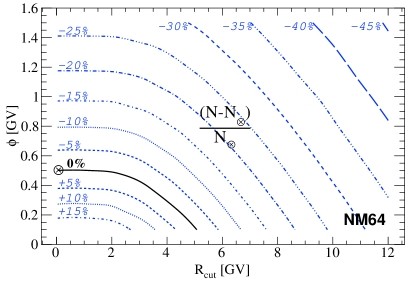
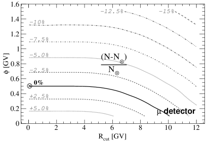
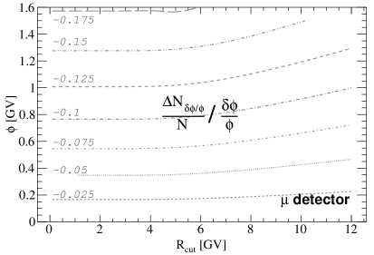
Figure 16: Left panels are calculated for NM64 and right panels for $\mu$ detectors. Top panels: Count rate relative variation $\Delta N/N_{\otimes}$ with respect to a reference count rate $N_{\otimes}=N(\phi=0.5,\,R_{c}=0)$. The relative variation (in %) are shown as iso-contours in the plane $(R_{c},\,\phi)$, with the 0%-isocontour (passing through the reference point $\otimes$) in black solid line. Bottom panels: scaling factor $f$ to infer the count rate relative variation $[\Delta N_{\delta\phi/\phi}/N](R_{c},\,\phi)$ for any modulation relative change $\delta\phi/\phi$ (for NM64, slight differences in the contours arise for values of $\delta\phi/\phi>20\%$ and factor $f<-0.3$). For instance, for a NM64 detector at $R_{c}=6.5$ GV and a solar modulation period $\phi=1.2$ GV, the scaling factor is $f=-0.25$, which reads: an increase of 5% (resp. 10%) in the modulation level $\phi$ translates in a decrease of $0.25\times 5\%=1.25\%$ (resp. 2.5%) in the detector count rate, and vice versa.

Table 9: Impact of different effects/input ingredients ($1^{\rm st}$ and$2^{\rm nd}$ columns) on the relative count rate calculation for NMs and $\mu$-like detectors ($4^{\rm th}$ and $5^{\rm th}$ columns), and on the uncertainty associated to the derived modulation parameter value ($6^{\rm th}$ and $7^{\rm th}$ columns). The first two rows, in italic, serve as a reference: they correspond to the maximum variation expected between periods of low and high solar activity, and low and high rigidity cut-off). The $3^{\rm rd}$ column provides the figure or section where the effect is discussed in the paper. See text for description.

Ingredient	Effect	​​​​​​​​Fig./Sect.​​​​​​​​​​​​​​	$\displaystyle\frac{\Delta N}{N}$		$\Delta\phi^{\ast}$ [MV]		Comment
			NM	$\mu$	NM	$\mu$
​​​​​Solar modulation​​​​​	$\phi\in$ [0.2,1.5] GV	Fig.16	[+15,-25]%	[+5,-10]%	-	-	w.r.t. $\mathit{\phi\!=\!0.5}$ GV
​​​Cut-off rigidity​​​	$R_{c}\in$ [0,10] GV	Fig.11	[+10,-20]%	[0,-5]%	-	-	w.r.t. $\mathit{R_{c}\!=\!5}$ GV
TOA flux	p and He CR data	Fig.12	$\pm 2\%$	$\pm 2\%$	$\pm 66$	$\pm 140$	$(t,\,R_{c},\,\phi)$-independent
	IS flux dispersion¶	Fig.12	$\pm 6\%$	$\pm 8\%$	$\pm 200$	$\pm 570$	$\Downarrow$
	Heavy species	Fig.1	$\pm 0.6\%$	$\pm 0.6\%$	$\pm 20$	$\pm 40$	Global norm. factor⋄
​​​Yield function​​​	Dispersion	Fig.12	$\lesssim\pm 4\%$	$<0.2\%$	$\lesssim 120$	$\lesssim 14$	$(R_{c},\,\phi)$ dependent
	Sigmoid$(R_{c},x\!=\!+\frac{\sigma}{0.1})$	Fig.13	-$2x\%$	-$0.5x\%$	+$66x$	+$35x$	For $R_{c}\gtrsim 5$ GV
Transfer	​​​​​$H(R_{c}\!\!+\!\!\Delta R_{c})$: $x\!\!=\!\!\frac{\!\!(\Delta R_{c}\!/\!R_{c})\!\!}{0.05}$	Fig.13	-$2x\%$	-$x\%$	+$66x$	+$71x$	For $R_{c}\gtrsim 5$ GV
function	- $R_{c}(t)$: $\frac{\Delta R}{R}\!\lesssim\!+0.2\%$/yr​​​​​​	§5.2.2	-0.4%/yr​​​​​​​​​	-0.1%/yr​​​​​​​​​	+13/yr​​​​​	+7/yr​​​	Depends on location
	​​​​​​- $R^{\rm eff}_{c}\!\rightarrow\!R^{\rm app}_{c}$: $\!+3\%$	§5.2.2	-1.2%	-0.3%	+40	+21	Depends on $R_{c}$
	Pressure	§5.3.1	$\pm 0.2\%$	$\pm 0.2\%$	$\pm 6$	$\pm 14$	After correction
Time-dep.	Temperature	§5.3.2	$\pm 0.5\%$	$\pm 4\%$	$\pm 15$	$\pm 290^{\ddagger}$	Not corrected
effects†	Vapour water	§5.3.3	$\pm 0.3\%$	$\pm 0.1\%$	$\pm 10$	$\pm 8$	Not corrected
	​​​​​​​​Snow coverage ($T\!\!=\!\!1$ yr)​​​​​​​	§5.3.4	-7%	-	+230	-	Not corrected
NM detector	Temperature	§5.4	+0.05%/∘C​​​​​​	-	-1.5/∘C​​​​​​	-	$(t,\,R_{c},\,\phi)$-independent
effects	$n$NM6 vs $m$NM64	§5.4	few %	-	$\sim 100$	-	$\Downarrow$
	Surroundings (hut)	§5.4	few %	-	$\sim 100$	-	Global norm. factor⋄

^∗ The variation $\Delta\phi$ of the modulation level is calculated for a detector at $R_{c}=5$ GV and $\phi=0.5$ GV:
refer to Fig. 16 to convert rate variations for any other $(R_{c},\,\phi$) condition.
^¶ Very conservative estimate (some IS fluxes are based on old CR data).
^⋄ Global normalisation factors can always be absorbed in the yield function normalisation.
^† Distributed data are either corrected or not corrected for these effects.
^‡ After correction, $\Delta N/N\sim 0.3\%$ (Dmitrieva et al., 2011), leading to $\Delta\phi\sim 22$ MV.

6.3 Abacus: count rates to solar modulation variations

To conclude, we propose a last figure and a table for a panoptic view of all the effects we have approached in this study. Actually, these plots provide a direct link between solar modulation level and count rate variations (and vice versa) for both NM64 and $\mu$ detectors.

The top panels of Fig. 16 provide the relative count rate variation in the $R_{c}-\phi$ plane, with respect to a reference point $N_{\otimes}(R_{c}=0,\phi=0.5$ GV). In addition to providing a global view of the expected count rate variation between detectors at different $R_{c}$ and for different solar periods, it also gives a flavour of the precision required in order to be sensitive to changes in the $\phi$ parameter: the count rate variation over a full solar cycle is smaller for $\mu$ detectors than for NMs, but the latter are more sensitive to any uncertainty on $R_{c}$ (location in the geomagnetic field) than the former.

The bottom panels of Fig. 16 go further in that direction, as they directly provide, for any value $(R_{c},\,\phi)$, how much variation $\Delta N/N$ to expect in the count rates, whenever the solar modulation changes by $\delta\phi/\phi$. This abacus usage is two-folds: first, on short term variations, it can directly be used to extract $\delta\phi/\phi$ from count rate variation in NM (or $\mu$) data; second, it can be used to estimate how much uncertainty is propagated in $\phi$ from the various uncertainties calculated on count rates.

This is what is gathered in Table 9: for each input/effect discussed in the paper, we provide (in addition to the section/figure where it was dealt with) the typical uncertainty obtained on $\Delta N/N$, and the associated $\Delta\phi$ calculated for an NM64 or $\mu$ detector at $R_{c}=5$ GV and a solar modulation level of $\phi=500$ MV (using Fig. 16). For $\phi$ calculations, the first thing to underline is that NM and $\mu$ detectors do not suffer the same amount of uncertainties, due to different sensitivities to the various effects explored. Moreover, there are no clear-cut ranking of these errors. Luckily, when interested in time series, time-independent normalisation effects can be absorbed in a normalisation factor (e.g., Usoskin et al., 2011): the latter accounts for differences in NM detector efficiency and their surroundings (last entries in table). The case of the IS fluxes (first entries in table) is peculiar, since different choices $i$ lead to an overall shift $\Delta\phi_{i}$ of the time series. For NMs, the main source of uncertainties are the seasonal snow effects (strength depending on position, some stations not affected), and the yield function dispersion (applicable for all stations). All other effects cannot be simply disregarded as they typically have a $5-10\%$ on $\phi$. For $\mu$ detectors, the main effect is that of the temperature variation, but after corrections, it is at the level of other uncertainties ($5-10\%$). Overall, $\mu$ detectors seem to suffer slightly less uncertainties than NM64, but of course the latter benefit from a much larger time and position coverage than the former.

6.4 Future works

The approach we have followed in this study could easily be extended to other types of ground-based measurements, by simply using the appropriate yield function for each type (e.g., ¹⁰Be production in ice cores, Herbst et al. 2010; ionisation measurements in the atmosphere, Bazilevskaya et al. 2008; etc.). In any case, one of the main challenge of such approaches is to obtain an accurate yield function. In that respect, the efforts to improve that of NMs should be pursued, given their role in the history of solar activity monitoring.

As underlined at the beginning of this study, our primary goal is to get time series of modulation parameters, taking advantage of the complementarity of NM count rates and TOA CR flux measurements. The above Table 9 provides a synthetic view of the difficulties. This table, and more importantly, the characterisation of the dependence of these uncertainties with $R_{c}$, ‘weather’ conditions for the stations, etc., should help decide which stations to consider to minimise the uncertainties in the $\phi$ calculations. This is the aim of our next study.

Appendix A IS flux parametrisation (p and He)

For completeness, we provide below all IS flux parametrisations $dJ^{\rm IS}/dT_{n}$ used in the paper. They are given for protons and heliums in unit of [m^-2 s^-1 sr^-1 (GeV/n)^-1]. The formulae are expressed in terms of:
- the rigidity $R$ (in GV)
- the kinetic energy per nucleon $T_{n}$ (in MeV/n)
- $\beta=v/c$.

• GM75 (Garcia-Munoz et al., 1975):

  $$J_{\rm p}(T_{n}) =9.9\,10^{11}\,\left(T_{n}+780\exp(-2.5\,10^{-4}\;T_{n})\right)^{-2.65};$$

  $$J_{\rm He}(T_{n}) =0.0525\times J_{\rm p}(T_{n}).$$

• B00+U05 (Burger et al., 2000; Usoskin et al., 2011):

  $$J_{\rm p}(R) =\frac{1.9\,10^{4}\;R^{-2.78}}{1+0.4866R^{-2.51}};$$

  $$J_{\rm He}(R) =0.38\times J_{\rm p}(R).$$

• L03 (Langner et al., 2003): using $x=\ln(T_{n})$,

  $$J_{\rm p}(T_{n}) =\!10^{3}\!\begin{cases}e^{[22.976-2.86x-1.5\,10^{3}/T_{n}]}\;\;(T_{n}\!\!>\!\!1000);\\ e^{[0.823-0.08x^{2}+1.105x-0.09202\sqrt{T_{n}}]}.\\ \end{cases}$$

  $$J_{\rm He}(T_{n}) =0.055\times J_{\rm p}(T_{n}).$$

• WH03 (Webber and Higbie, 2003):

  $$J_{\rm p}(T_{n}) =\frac{10^{13}}{1.89\;T_{n}^{2.8}+5.05\,10^{4}\;T_{n}^{1.58}+9.33\,10^{7}\;T_{n}^{0.26}};$$

  $$J_{\rm He}(T_{n}) =0.056\times J_{\rm p}(T_{n}).$$

• S07 (Shikaze et al., 2007):

  $$J_{\rm p}(R) =1.94\cdot 10^{4}\times\beta^{0.7}R^{-2.76};$$

  $$J_{\rm He}(R) =0.71\cdot 10^{4}\times\beta^{0.5}R^{-2.78}.$$

• WH09 (Webber and Higbie, 2009): using $x=\ln(T_{n})$,

  $$J_{\rm p}(T_{n}) =\!10^{3}\!\begin{cases}e^{-51.68\ln(x)^{2}+\frac{103.6}{x^{-1/2}}-\frac{709.7}{x}+\frac{1162.}{x^{2}}}\;\;(T_{n}\!\!>\!\!1000);\\ e^{-124.5-51.84\ln(x)^{2}+\frac{131.6}{x^{-1/2}}-\frac{241.7}{x}+\frac{376.7}{x^{2}}}.\\ \end{cases}$$

  $$J_{\rm He}(T_{n}) =0.0605\times J_{\rm p}(T_{n}).$$

• BO11​ (Badhwar and O’Neill 1996; O’Neill 2006; O’Neill 2010):​​​

  $$J_{\rm p}(T_{n}) =4.502\cdot 10^{12}\times\beta^{-1.7708}\;(T_{n}+938)^{-2.7748};$$

  $$J_{\rm He}(T_{n}) =2.472\cdot 10^{11}\times\beta^{-2.2502}\;(T_{n}+938)^{-2.7796}.$$

• This paper $\equiv J_{\rm ref}$:

  $$J_{\rm p}(R) =2.335\cdot 10^{4}\times\beta^{1.1}R^{-2.839};$$

  $$J_{\rm He}(R) =0.7314\cdot 10^{4}\times\beta^{0.77}R^{-2.782}.$$

Appendix B Yield for NM and $\mu$ detectors

Yield functions are given below for protons $Y_{\rm p}$, and in some cases for heliums $Y_{\rm He}$. If not available, a rescaled version of $Y_{\rm p}$ is used, see Eq. (13). The yield functions are given in unit of [m² sr], and are expressed in terms of
- the grammage $g$ (in g cm^-2)
- the altitude $h$ (in m) w.r.t. to sea level
- the rigidity $R$ (in GV)
- the kinetic energy $T$ (in GeV)
- the kinetic energy per nucleon $T_{/n}$ (in GeV/n)
- $\gamma=E_{\rm tot}/m$.

B.1 NM64 yield parametrisations

The yields are given for a 6NM64 neutron monitor. For an $x$NM64 device, the yield functions below are multiplied by $x/6$.

Note that Mishev et al. (2013) proposed a correction factor $G$ to account for the geometrical factor of the NM effective size (in the context of yield functions calculated in MC simulations). This correction, fitted on their Fig.2, reads:

$$G=\max\left[1,\,1.4\times\log_{10}\left(\frac{T_{/n}}{2.39}\right)\right].$$ (22)

To apply this correction, the below MC-based yield functions (i.e. CD00, F08, M09) can simply be multiplied by $G$. This correction is already accounted for in M13, and does not intervene in NM ‘count rate’-based formulae (N89, CL12).

• N89 (Nagashima et al., 1989, 1990): using $x=\frac{g}{1033}$,

  $${\cal Y}_{\rm p}(g,\gamma) =10^{4}\,\exp\left(-2.2\,x^{1.62}-\frac{12.7\,x^{0.5}}{\ln(\gamma)^{0.42}}\right).$$

• CD00 (Clem, 1999; Clem and Dorman, 2000): the fit is adapted from Caballero-Lopez and Moraal (2012),

  $${\cal Y}_{\rm p}^{\rm asl}(R) =2\,10^{-2}\,\left(0.45^{1.4}+R^{1.4}\right)^{-20.79}R^{30}.$$

  A power-law extrapolation of slope $0.5$ is used above $R>100$ GV.

• F08 (Flückiger et al., 2008):

  $${\cal Y}_{\rm p}(g,R) =10^{\sum_{i=0}^{4}\sum_{j=0}^{4}a_{ij}\,g^{i}\,(\log_{10}(R))^{j}}.$$

  with

  $$\begin{cases}a_{0j}=~{}~{}~{}~{}~{}~{}~{}~{}~{}~{}\{0.7983,\,2.859,\,-2.060,\,0.5654\};\\ a_{1j}=10^{-2}\times\{-0.6985,\,1.188,\,-0.9264,\,0.2169\};\\ a_{2j}=10^{-5}\times\{0.3593,\,-1.516,\,1.522,\,-0.4214\};\\ a_{3j}=10^{-9}\times\{-1.950,\,7.969,\,-8.508,\,2.491\}.\end{cases}$$ (23)

  A power-law extrapolation of slope $0.5$ is used above $R>100$ GV.

• M09 (Matthiä et al., 2009; Matthiä, 2009): using $I=\log_{10}(T)+1.94$ and $J=\log_{10}(T)+2.2$,

  $${\cal Y}_{\rm p}^{\rm asl}(R) =2\pi\,10^{-4}\times 10^{-44.40-22.62I+1.007I^{2}+61.01\sqrt{I}};$$

  $${\cal Y}_{\rm He}^{\rm asl}(R) =2\pi\,10^{-4}\times 10^{-50.78-16.32J+0.409J^{2}+56.44\sqrt{J}}.$$

  Above $T_{/n}>500$ GeV/n, a power-law extrapolation is used (based on two points calculated at 450 and 500 GeV/n).

• CL12 (Caballero-Lopez and Moraal, 2012):

  $${\cal Y}_{\rm p}^{\rm asl}(R) =2\,10^{-2}\,\left(2^{1.45}+R^{1.45}\right)^{-4.696}R^{7.7};$$

  $$\frac{{\cal Y}_{\rm He}}{{\cal Y}_{\rm p}}^{\rm asl}(R) =2\,\left(0.45^{1.4}+R^{1.4}\right)^{-7.143}R^{10}.$$

• M13 (Mishev et al., 2013): using $I=\log_{10}(R)+0.469$ and $J=\log_{10}(R)+0.1$, we fit their data (Table 1) with

  $${\cal Y}_{\rm p}^{\rm asl}(R) =10^{-19.86-13.79I+0.963I^{2}+30.56\sqrt{I}};$$

  $${\cal Y}_{\rm He}^{\rm asl}(R) =4\times 10^{-19.83-13.81J+0.971J^{2}+30.58\sqrt{J}}.$$

• This paper: Eq. (12) and Table 5. A power-law extrapolation is used above $R>200$ GV (based on two points calculated at 150 GV and 200 GV).

B.2 $\mu$ detector yield parametrisations

• PD02 (Poirier and D’Andrea, 2002): the fit is from Caballero-Lopez and Moraal (2012).

  $$Y_{\rm p}^{\rm asl}(R) =1.07\cdot 10^{-1}\,\left(1+R\right)^{-27.15}R^{28}.$$

• This paper (Eq. 12 and Table 6): using $I=\log_{10}(T_{/n})+2.068$,

  $$Y_{\rm p}(h,T_{/n}) =e^{0.00025h}\times 10^{(0.9116I-664.1I^{-5.818}-2.755)}.$$

References

- Ahluwalia (2013) H. S. Ahluwalia. Sunspot numbers, interplanetary magnetic field, and cosmic ray intensity at earth: Nexus for the twentieth century. Advances in Space Research, 52:2112–2118, December 2013. doi: 10.1016/j.asr.2013.09.009.
- Ahn et al. (2010) H. S. Ahn, P. Allison, M. G. Bagliesi, et al. Discrepant Hardening Observed in Cosmic-ray Elemental Spectra. ApJ, 714:L89–L93, May 2010. doi: 10.1088/2041-8205/714/1/L89.
- AMS Collaboration et al. (2000a) AMS Collaboration, J. Alcaraz, B. Alpat, G. Ambrosi, et al. Cosmic protons. Physics Letters B, 490:27–35, September 2000a. doi: 10.1016/S0370-2693(00)00970-9.
- AMS Collaboration et al. (2000b) AMS Collaboration, J. Alcaraz, B. Alpat, G. Ambrosi, et al. Helium in near Earth orbit. Physics Letters B, 494:193–202, November 2000b. doi: 10.1016/S0370-2693(00)01193-X.
- AMS Collaboration et al. (2002) AMS Collaboration, M. Aguilar, J. Alcaraz, J. Allaby, B. Alpat, G. Ambrosi, H. Anderhub, L. Ao, A. Arefiev, P. Azzarello, and et al. The Alpha Magnetic Spectrometer (AMS) on the International Space Station: Part I - results from the test flight on the space shuttle. Phys. Rep., 366:331–405, August 2002. doi: 10.1016/S0370-1573(02)00013-3.
- AMS Collaboration et al. (2011) AMS Collaboration, M. Aguilar, J. Alcaraz, J. Allaby, et al. Isotopic Composition of Light Nuclei in Cosmic Rays: Results from AMS-01. ApJ, 736:105, August 2011. doi: 10.1088/0004-637X/736/2/105.
- Babcock (1961) H. W. Babcock. The Topology of the Sun’s Magnetic Field and the 22-YEAR Cycle. ApJ, 133:572, March 1961. doi: 10.1086/147060.
- Badhwar and O’Neill (1994) G. D. Badhwar and P. M. O’Neill. Long-term modulation of galactic cosmic radiation and its model for space exploration. Advances in Space Research, 14:749–757, October 1994. doi: 10.1016/0273-1177(94)90537-1.
- Badhwar and O’Neill (1996) G. D. Badhwar and P. M. O’Neill. Galactic cosmic radiation model and its applications. Advances in Space Research, 17:7, 1996. doi: 10.1016/0273-1177(95)00507-B.
- Bazilevskaya et al. (2008) G. A. Bazilevskaya, I. G. Usoskin, E. O. Flückiger, R. G. Harrison, L. Desorgher, R. Bütikofer, M. B. Krainev, V. S. Makhmutov, Y. I. Stozhkov, A. K. Svirzhevskaya, N. S. Svirzhevsky, and G. A. Kovaltsov. Cosmic Ray Induced Ion Production in the Atmosphere. Space Sci. Rev., 137:149–173, June 2008. doi: 10.1007/s11214-008-9339-y.
- Bercovitch and Robertson (1965) M. Bercovitch and B. C. Robertson. Meteorological factors affecting the counting rate of neutron monitors. In International Cosmic Ray Conference, volume 1 of International Cosmic Ray Conference, page 489, 1965.
- Berkova et al. (2012) M. Berkova, A. Belov, E. Eroshenko, and V. Yanke. Temperature effect of muon component and practical questions of how to take into account in real time. Astrophysics and Space Sciences Transactions, 8:41–44, December 2012. doi: 10.5194/astra-8-41-2012.
- Berkova et al. (2011) M. D. Berkova, A. V. Belov, E. A. Eroshenko, and V. G. Yanke. Temperature effect of the muon component and practical questions for considering it in real time. Bulletin of the Russian Academy of Science, Phys., 75:820–824, June 2011. doi: 10.3103/S1062873811060086.
- Bieber et al. (2013) J. Bieber, J. Clem, P. Evenson, S. Oh, and R. Pyle. Continued decline of South Pole neutron monitor counting rate. Journal of Geophysical Research (Space Physics), 118:6847–6851, November 2013. doi: 10.1002/2013JA018915.
- Bieber and Evenson (1995) J. W. Bieber and P. Evenson. Spaceship Earth - An Optimized Network of Neutron Monitors. International Cosmic Ray Conference, 4:1316, 1995.
- Bieber et al. (1997) J. W. Bieber, J. Clem, and P. Evenson. Efficient Computation of Apparent Cutoffs. International Cosmic Ray Conference, 2:389, 1997.
- Bieber et al. (2007) J. W. Bieber, J. Clem, D. Desilets, P. Evenson, D. Lal, C. Lopate, and R. Pyle. Long-term decline of South Pole neutron rates. Journal of Geophysical Research (Space Physics), 112:A12102, December 2007. doi: 10.1029/2006JA011894.
- Binns et al. (1989) W. R. Binns, T. L. Garrard, P. S. Gibner, M. H. Israel, M. P. Kertzman, J. Klarmann, B. J. Newport, E. C. Stone, and C. J. Waddington. Abundances of ultraheavy elements in the cosmic radiation - Results from HEAO 3. ApJ, 346:997–1009, November 1989. doi: 10.1086/168082.
- Bobik et al. (2006) P. Bobik, G. Boella, M. J. Boschini, M. Gervasi, D. Grandi, K. Kudela, S. Pensotti, and P. G. Rancoita. Magnetospheric transmission function approach to disentangle primary from secondary cosmic ray fluxes in the penumbra region. Journal of Geophysical Research (Space Physics), 111:A05205, May 2006. doi: 10.1029/2005JA011235.
- Bobik et al. (2009) P. Bobik, G. Boella, M. J. Boschini, M. Gervasi, D. Grandi, K. Kudela, S. Pensotti, and P. G. Rancoita. Fluxes and nuclear abundances of cosmic rays inside the magnetosphere using a transmission function approach. Advances in Space Research, 43:385–393, February 2009. doi: 10.1016/j.asr.2008.11.020.
- Boella et al. (1998) G. Boella, M. Gervasi, M. A. C. Potenza, P. G. Rancoita, and I. Usoskin. Modulated antiproton fluxes for interstellar production models. Astroparticle Physics, 9:261–267, October 1998. doi: 10.1016/S0927-6505(98)00022-X.
- Boezio et al. (1999) M. Boezio, P. Carlson, T. Francke, et al. The Cosmic-Ray Proton and Helium Spectra between 0.4 and 200 GV. ApJ, 518:457–472, June 1999. doi: 10.1086/307251.
- Buchvarova and Draganov (2013) M. Buchvarova and D. Draganov. Cosmic-Ray Spectrum Approximation Model: Experimental Results and Comparison with Other Models. Sol. Phys., 284:599–614, June 2013. doi: 10.1007/s11207-012-0157-8.
- Buchvarova and Velinov (2010) M. Buchvarova and P. I. Y. Velinov. Empirical model of cosmic ray spectrum in energy interval 1 MeV-100 GeV during 11-year solar cycle. Advances in Space Research, 45:1026–1034, April 2010. doi: 10.1016/j.asr.2009.12.014.
- Buchvarova et al. (2011) M. Buchvarova, P. I. Y. Velinov, and I. Buchvarov. Model approximation of cosmic ray spectrum. Planet. Space Sci., 59:355–363, March 2011. doi: 10.1016/j.pss.2011.01.001.
- Burger et al. (2000) R. A. Burger, M. S. Potgieter, and B. Heber. Rigidity dependence of cosmic ray proton latitudinal gradients measured by the Ulysses spacecraft: Implications for the diffusion tensor. J. Geophys. Res., 105:27447–27456, December 2000. doi: 10.1029/2000JA000153.
- Bütikofer et al. (2008) R. Bütikofer, E. O. Flückiger, and L. Desorgher. Characteristics of near real-time cutoff calculations on a local and global scale. In International Cosmic Ray Conference, volume 1 of International Cosmic Ray Conference, pages 769–772, 2008.
- Caballero-Lopez and Moraal (2004) R. A. Caballero-Lopez and H. Moraal. Limitations of the force field equation to describe cosmic ray modulation. Journal of Geophysical Research (Space Physics), 109:A01101, January 2004. doi: 10.1029/2003JA010098.
- Caballero-Lopez and Moraal (2012) R. A. Caballero-Lopez and H. Moraal. Cosmic-ray yield and response functions in the atmosphere. Journal of Geophysical Research (Space Physics), 117:A12103, December 2012. doi: 10.1029/2012JA017794.
- Carmichael et al. (1965) H. Carmichael, M. Bercovitch, J. F. Steljes, and M. Magidin. Latitude survey in North America. International Cosmic Ray Conference, 1:553, 1965.
- Cecchini and Spurio (2012) S. Cecchini and M. Spurio. Atmospheric muons: experimental aspects. Geoscientific Instrumentation, Methods and Data Systems, 1:185–196, November 2012. doi: 10.5194/gi-1-185-2012.
- Chasson et al. (1966) R. L. Chasson, V. J. Kisselbach, and T. C. Sharma. Atmospheric water vapor and attenuation of the cosmic-ray nucleonic component. J. Geophys. Res., 71:5183–5184, November 1966. doi: 10.1029/JZ071i021p05183.
- Cheminet et al. (2012a) A. Cheminet, V. Lacoste, V. Gressier, G. Hubert, A. Martin, and M. Pépino. Characterization of the IRSN neutron multisphere spectrometer (HERMEIS) at European standard calibration fields. Journal of Instrumentation, 7:C4007, April 2012a. doi: 10.1088/1748-0221/7/04/C04007.
- Cheminet et al. (2012b) A. Cheminet, V. Lacoste, G. Hubert, D. Boscher, D. Boyer, and J. Poupeney. Experimental Measurements of the Cosmic-Ray Induced Neutron Spectra at Various Mountain Altitudes With HERMEIS. IEEE Transactions on Nuclear Science, 59:1722–1730, August 2012b. doi: 10.1109/TNS.2012.2201500.
- Cheminet et al. (2013a) A. Cheminet, G. Hubert, V. Lacoste, and D. Boscher. Measurements and Monte Carlo Simulations of the spectral variations of the cosmic-ray induced neutrons at the Pic du Midi over a two-year period. Radiation Protection Dosimetry, 2013a. doi: 10.1093/rpd/nct330.
- Cheminet et al. (2013b) A. Cheminet, G. Hubert, V. Lacoste, D. Maurin, and L. Derome. Cosmic ray solar modulation and Forbush decrease analyses based on atmospheric neutron spectrometry at mountain altitude and GEANT4 simulations of extensive air showers. Journal of Geophysical Research (Space Physics), 118:7488–7496, December 2013b. doi: 10.1002/2013JA019166.
- Cheminet et al. (2013c) A. Cheminet, G. Hubert, V. Lacoste, R. Velazco, and D. Boscher. Characterization of the Neutron Environment and SEE Investigations at the CERN-EU High Energy Reference Field and at the Pic du Midi. IEEE Transactions on Nuclear Science, 60:2411–2417, August 2013c. doi: 10.1109/TNS.2012.2231699.
- Chilingarian and Karapetyan (2011) A. Chilingarian and T. Karapetyan. Calculation of the barometric coefficients at the start of the 24th solar activity cycle for particle detectors of Aragats Space Environmental Center. Advances in Space Research, 47:1140–1146, April 2011. doi: 10.1016/j.asr.2010.12.001.
- Clem (1999) J. Clem. Atmospheric Yield Functions and the Response to Secondary Particles of Neutron Monitors. International Cosmic Ray Conference, 7:317, 1999.
- Clem and Dorman (2000) J. M. Clem and L. I. Dorman. Neutron Monitor Response Functions. Space Sci. Rev., 93:335–359, July 2000. doi: 10.1023/A:1026508915269.
- Clem et al. (1997) J. M. Clem, J. W. Bieber, P. Evenson, D. Hall, J. E. Humble, and M. Duldig. Contribution of obliquely incident particles to neutron monitor counting rate. J. Geophys. Res., 102:26919–26926, December 1997. doi: 10.1029/97JA02366.
- Cooke et al. (1991) D. J. Cooke, J. E. Humble, M. A. Shea, D. F. Smart, and N. Lund. On cosmic-ray cut-off terminology. Nuovo Cimento C Geophysics Space Physics C, 14:213–234, June 1991. doi: 10.1007/BF02509357.
- Davis et al. (2001) A. J. Davis, R. A. Mewaldt, C. M. S. Cohen, A. C. Cummings, J. S. George, R. A. Leske, E. C. Stone, M. E. Wiedenbeck, N. E. Yanasak, E. R. Christian, T. T. von Rosenvinge, W. R. Binns, and P. L. Hink. Solar minimum spectra of galactic cosmic rays and their implications for models of the near-earth radiation environment. J. Geophys. Res., 106:29979–29988, December 2001. doi: 10.1029/2000JA000325.
- de Nolfo et al. (2000) G. A. de Nolfo, L. M. Barbier, E. R. Christian, A. J. Davis, R. L. Golden, M. Hof, K. E. Krombel, A. W. Labrador, W. Menn, R. A. Mewaldt, J. W. Mitchell, J. F. Ormes, I. L. Rasmussen, O. Reimer, S. M. Schindler, M. Simon, S. J. Stochaj, R. E. Streitmatter, and W. R. Webber. A measurement of cosmic ray deuterium from 0.5-2.9 GeV/nucleon. In R. A. Mewaldt, J. R. Jokipii, M. A. Lee, E. Möbius, and T. H. Zurbuchen, editors, Acceleration and Transport of Energetic Particles Observed in the Heliosphere, volume 528 of American Institute of Physics Conference Series, pages 425–428, September 2000. doi: 10.1063/1.1324352.
- de Nolfo et al. (2006) G. A. de Nolfo, I. V. Moskalenko, W. R. Binns, E. R. Christian, A. C. Cummings, A. J. Davis, J. S. George, P. L. Hink, M. H. Israel, R. A. Leske, M. Lijowski, R. A. Mewaldt, E. C. Stone, A. W. Strong, T. T. von Rosenvinge, M. E. Wiedenbeck, and N. E. Yanasak. Observations of the Li, Be, and B isotopes and constraints on cosmic-ray propagation. Advances in Space Research, 38:1558–1564, January 2006. doi: 10.1016/j.asr.2006.09.008.
- Desorgher et al. (2009) L. Desorgher, K. Kudela, E. O. Flückiger, R. Bütikofer, M. Storini, and V. Kalegaev. Comparison of Earth’s magnetospheric magnetic field models in the context of cosmic ray physics. Acta Geophysica, 57:75–87, March 2009. doi: 10.2478/s11600-008-0065-3.
- Dmitrieva et al. (2011) A. N. Dmitrieva, R. P. Kokoulin, A. A. Petrukhin, and D. A. Timashkov. Corrections for temperature effect for ground-based muon hodoscopes. Astroparticle Physics, 34:401–411, January 2011. doi: 10.1016/j.astropartphys.2010.10.013.
- Dorman (1974) L. I. Dorman. Cosmic rays: Variations and space explorations. Amsterdam: North-Holland, and New York: Elsevier, 1974, 1974.
- Dorman (2004) L. I. Dorman. Cosmic Rays in the Earth’s Atmosphere and Underground. Astrophysics and Space Science Library, Vol. 303. Kluwer Academic Publishers, Dordrecht, 2004.
- Dorman (2009) L. I. Dorman. Cosmic Rays in Magnetospheres of the Earth and other Planets. Astrophysics and Space Science Library, Vol. 358. Springer, 2009. ISBN: 978-1-4020-9238-1, 2009.
- Dorman et al. (2000) L. I. Dorman, G. Villoresi, N. Iucci, M. Parisi, M. I. Tyasto, O. A. Danilova, and N. G. Ptitsyna. Cosmic ray survey to Antarctica and coupling functions for neutron component near solar minimum (1996-1997) 3. Geomagnetic effects and coupling functions. J. Geophys. Res., 105:21047–21056, 2000. doi: 10.1029/2000JA900051.
- Dorman et al. (2008) L. I. Dorman, O. A. Danilova, N. Iucci, M. Parisi, N. G. Ptitsyna, M. I. Tyasto, and G. Villoresi. Effective non-vertical and apparent cutoff rigidities for a cosmic ray latitude survey from Antarctica to Italy in minimum of solar activity. Advances in Space Research, 42:510–516, August 2008. doi: 10.1016/j.asr.2007.04.032.
- Duldig (2000) M. L. Duldig. Muon Observations. Space Sci. Rev., 93:207–226, July 2000. doi: 10.1023/A:1026596529381.
- Engelmann et al. (1990) J. J. Engelmann, P. Ferrando, A. Soutoul, P. Goret, and E. Juliusson. Charge composition and energy spectra of cosmic-ray nuclei for elements from Be to NI - Results from HEAO-3-C2. A&A, 233:96–111, July 1990.
- Ferrando et al. (1988) P. Ferrando, J. J. Engelmann, P. Goret, L. Koch-Miramond, and N. Petrou. Measurement of the isotopic composition of cosmic-rays at 3 GeV/n using a new geomagnetic method. A&A, 193:69–80, March 1988.
- Flückiger et al. (1983) E. O. Flückiger, D. F. Smart, and M. A. Shea. The effect of local perturbations of the geomagnetic field on cosmic ray cutoff rigidities at Jungfraujoch and Kiel. J. Geophys. Res., 88:6961–6928, September 1983. doi: 10.1029/JA088iA09p06961.
- Flückiger et al. (1986) E. O. Flückiger, D. F. Smart, and M. A. Shea. A procedure for estimating the changes in cosmic ray cutoff rigidities and asymptotic directions at low and middle latitudes during periods of enhanced geomagnetic activity. J. Geophys. Res., 91:7925–7930, July 1986. doi: 10.1029/JA091iA07p07925.
- Flückiger et al. (2003) E. O. Flückiger, R. Buetikofer, L. Desorgher, and M. R. Moser. Global Cosmic Ray Cutoff Rigidities over the Past 2000 Years. In International Cosmic Ray Conference, volume 7 of International Cosmic Ray Conference, page 4229, July 2003.
- Flückiger et al. (2008) E. O. Flückiger, M. R. Moser, B. Pirard, and et al. A parameterized neutron monitor yield function for space weather applications. In International Cosmic Ray Conference, volume 1 of International Cosmic Ray Conference, pages 289–292, 2008.
- Garcia-Munoz et al. (1975) M. Garcia-Munoz, G. M. Mason, and J. A. Simpson. The anomalous He-4 component in the cosmic-ray spectrum at below approximately 50 MeV per nucleon during 1972-1974. ApJ, 202:265–275, November 1975. doi: 10.1086/153973.
- Geant4 Collaboration et al. (2003) Geant4 Collaboration, S. Agostinelli, et al. Geant4-a simulation toolkit. Nuclear Instruments and Methods in Physics Research A, 506:250–303, July 2003.
- George et al. (2009) J. S. George, K. A. Lave, M. E. Wiedenbeck, W. R. Binns, A. C. Cummings, A. J. Davis, G. A. de Nolfo, P. L. Hink, M. H. Israel, R. A. Leske, R. A. Mewaldt, L. M. Scott, E. C. Stone, T. T. von Rosenvinge, and N. E. Yanasak. Elemental Composition and Energy Spectra of Galactic Cosmic Rays During Solar Cycle 23. ApJ, 698:1666–1681, June 2009. doi: 10.1088/0004-637X/698/2/1666.
- Gleeson and Axford (1967) L. J. Gleeson and W. I. Axford. Cosmic Rays in the Interplanetary Medium. ApJ, 149:L115, September 1967. doi: 10.1086/180070.
- Gleeson and Axford (1968) L. J. Gleeson and W. I. Axford. Solar Modulation of Galactic Cosmic Rays. ApJ, 154:1011, December 1968. doi: 10.1086/149822.
- Hatton and Carimichael (1964) C. J. Hatton and H. Carimichael. Experimental Investigation of the NM-64 Neutron Monitor. Canadian Journal of Physics, 42:2443–2472, December 1964. doi: 10.1139/p64-222.
- Hatton and Griffiths (1968) C. J. Hatton and W. K. Griffiths. Barometric coefficients of multiplicities in neutron monitors. J. Geophys. Res., 73:7503–7509, December 1968. doi: 10.1029/JA073i023p07503.
- Herbst et al. (2010) K. Herbst, A. Kopp, B. Heber, F. Steinhilber, H. Fichtner, K. Scherer, and D. Matthiä. On the importance of the local interstellar spectrum for the solar modulation parameter. Journal of Geophysical Research (Space Physics), 115, July 2010. doi: 10.1029/2009JD012557.
- Herbst et al. (2013) K. Herbst, A. Kopp, and B. Heber. Influence of the terrestrial magnetic field geometry on the cutoff rigidity of cosmic ray particles. Annales Geophysicae, 31:1637–1643, October 2013. doi: 10.5194/angeo-31-1637-2013.
- Hubert et al. (2013) G. Hubert, R. Velazco, C. Federico, A. Cheminet, C. Silva-Cardenas, L. V. E. Caldas, F. Pancher, V. Lacoste, F. Palumbo, W. Mansour, L. Artola, F. Pineda, and S. Duzellier. Continuous High-Altitude Measurements of Cosmic Ray Neutrons and SEU/MCU at Various Locations: Correlation and Analyses Based-On MUSCA SEP(3). IEEE Transactions on Nuclear Science, 60:2418–2426, August 2013. doi: 10.1109/TNS.2013.2240697.
- Indriolo and McCall (2012) N. Indriolo and B. J. McCall. Investigating the Cosmic-Ray Ionization Rate in the Galactic Diffuse Interstellar Medium through Observations of H+ 3. ApJ, 745:91, January 2012. doi: 10.1088/0004-637X/745/1/91.
- Iucci et al. (2000) N. Iucci, G. Villoresi, L. I. Dorman, and M. Parisi. Cosmic ray survey to Antarctica and coupling functions for neutron component near solar minimum (1996-1997) 2. Determination of meteorological effects. J. Geophys. Res., 105:21035–21046, 2000. doi: 10.1029/2000JA900050.
- James and Roos (1975) F. James and M. Roos. Minuit - a system for function minimization and analysis of the parameter errors and correlations. Computer Physics Communications, 10:343–367, December 1975. doi: 10.1016/0010-4655(75)90039-9.
- Jokipii (1966) J. R. Jokipii. Cosmic-Ray Propagation. I. Charged Particles in a Random Magnetic Field. ApJ, 146:480, November 1966. doi: 10.1086/148912.
- Keith et al. (1968) J. E. Keith, R. W. Peterson, R. L. Tjonaman, and J. R. Wang. Cosmic-ray neutron monitor yield functions, gross transformation, and nucleonic component mean free paths. J. Geophys. Res., 73:353–360, January 1968. doi: 10.1029/JA073i001p00353.
- Kim et al. (2013) K. C. Kim, K. Abe, H. Fuke, et al. Cosmic ray 2H/1H ratio measured from BESS in 2000 during solar maximum. Advances in Space Research, 51:234–237, January 2013. doi: 10.1016/j.asr.2012.01.015.
- Korotkov et al. (2013) V. Korotkov, M. Berkova, A. Belov, E. Eroshenko, V. Yanke, and R. Pyle. Procedure to emend neutron monitor data that are affected by snow accumulations on and around the detector housing. Journal of Geophysical Research (Space Physics), 118:6852–6857, November 2013. doi: 10.1002/2013JA018647.
- Korotkov et al. (2011) V. K. Korotkov, M. D. Berkova, A. V. Belov, E. A. Eroshenko, P. G. Kobelev, and V. G. Yanke. Effect of snow in cosmic ray variations and methods for taking it into consideration. Geomagnetism and Aeronomy, 51:247–253, April 2011. doi: 10.1134/S0016793211020095.
- Kremer et al. (1999) J. Kremer, M. Boezio, M. L. Ambriola, et al. Measurements of Ground-Level Muons at Two Geomagnetic Locations. Physical Review Letters, 83:4241–4244, November 1999. doi: 10.1103/PhysRevLett.83.4241.
- Krüger and Moraal (2005) H. Krüger and H. Moraal. Environmental effects on neutron monitors. International Cosmic Ray Conference, 2:477, 2005.
- Krüger and Moraal (2010) H. Krüger and H. Moraal. A calibration neutron monitor: Statistical accuracy and environmental sensitivity. Advances in Space Research, 46:1394–1399, December 2010. doi: 10.1016/j.asr.2010.07.008.
- Krüger and Moraal (2011) H. Krüger and H. Moraal. The Sensitivity of Neutron Monitor Counting Rate to Atmospheric Humidity. International Cosmic Ray Conference, 11:340, 2011.
- Krüger and Moraal (2013) H. Krüger and H. Moraal. Neutron monitor calibrations: progress report. Journal of Physics Conference Series, 409(1):012171, February 2013. doi: 10.1088/1742-6596/409/1/012171.
- Krüger et al. (2003) H. Krüger, H. Moraal, J. W. Bieber, J. M. Clem, P. A. Evenson, K. R Pyle, M. L. Duldig, and J. E. Humble. First Results of a Mobile Neutron Monitor to Intercalibrate the Worldwide Network. International Cosmic Ray Conference, 6:3441, July 2003.
- Krüger et al. (2008) H. Krüger, H. Moraal, J. W. Bieber, J. M. Clem, P. A. Evenson, K. R. Pyle, M. L. Duldig, and J. E. Humble. A calibration neutron monitor: Energy response and instrumental temperature sensitivity. Journal of Geophysical Research (Space Physics), 113:A08101, August 2008. doi: 10.1029/2008JA013229.
- Kubyshkina et al. (2009) M. Kubyshkina, V. Sergeev, N. Tsyganenko, V. Angelopoulos, A. Runov, H. Singer, K. H. Glassmeier, H. U. Auster, and W. Baumjohann. Toward adapted time-dependent magnetospheric models: A simple approach based on tuning the standard model. Journal of Geophysical Research (Space Physics), 114:A00C21, April 2009. doi: 10.1029/2008JA013547.
- Kudela et al. (2008) K. Kudela, R. Bučík, and P. Bobík. On transmissivity of low energy cosmic rays in disturbed magnetosphere. Advances in Space Research, 42:1300–1306, October 2008. doi: 10.1016/j.asr.2007.09.033.
- L3 Collaboration et al. (2004) L3 Collaboration, P. Achard, O. Adriani, et al. Measurement of the atmospheric muon spectrum from 20 to 3000 GeV. Physics Letters B, 598:15–32, September 2004. doi: 10.1016/j.physletb.2004.08.003.
- Langner et al. (2003) U. W. Langner, M. S. Potgieter, and W. R. Webber. Modulation of cosmic ray protons in the heliosheath. Journal of Geophysical Research (Space Physics), 108:8039, October 2003. doi: 10.1029/2003JA009934.
- Lave et al. (2013) K. A. Lave, M. E. Wiedenbeck, W. R. Binns, E. R. Christian, A. C. Cummings, A. J. Davis, G. A. de Nolfo, M. H. Israel, R. A. Leske, R. A. Mewaldt, E. C. Stone, and T. T. von Rosenvinge. Galactic Cosmic-Ray Energy Spectra and Composition during the 2009-2010 Solar Minimum Period. ApJ, 770:117, June 2013. doi: 10.1088/0004-637X/770/2/117.
- Lodders (2003) K. Lodders. Solar System Abundances and Condensation Temperatures of the Elements. ApJ, 591:1220–1247, July 2003. doi: 10.1086/375492.
- Masías-Meza et al. (2012) J. J. Masías-Meza, X. Bertou, and S. Dasso. Geomagnetic effects on cosmic ray propagation for different conditions. In C. H. Mandrini and D. F. Webb, editors, IAU Symposium, volume 286 of IAU Symposium, pages 234–237, July 2012. doi: 10.1017/S1743921312004899.
- Matthiä (2009) D. Matthiä. The Radiation Environment in the Lower Atmosphere A Numerical Approach. PhD thesis, Mathematisch-Naturwissenschaftliche Fakultät der Christian-Albrechts-Universität zu Kiel, 2009.
- Matthiä et al. (2009) D. Matthiä, B. Heber, G. Reitz, M. Meier, L. Sihver, T. Berger, and K. Herbst. Temporal and spatial evolution of the solar energetic particle event on 20 January 2005 and resulting radiation doses in aviation. Journal of Geophysical Research (Space Physics), 114:A08104, August 2009. doi: 10.1029/2009JA014125.
- Matthiä et al. (2013) D. Matthiä, T. Berger, A. I. Mrigakshi, and G. Reitz. A ready-to-use galactic cosmic ray model. Advances in Space Research, 51:329–338, February 2013. doi: 10.1016/j.asr.2012.09.022.
- Maurin et al. (2013) D. Maurin, F. Melot, and R. Taillet. A database of charged cosmic rays. ArXiv e-prints, February 2013.
- Menn et al. (2000) W. Menn, M. Hof, O. Reimer, et al. The Absolute Flux of Protons and Helium at the Top of the Atmosphere Using IMAX. ApJ, 533:281–297, April 2000. doi: 10.1086/308645.
- Mishev and Velinov (2011) A. L. Mishev and P. I. Y. Velinov. Normalized ionization yield function for various nuclei obtained with full Monte Carlo simulations. Advances in Space Research, 48:19–24, July 2011. doi: 10.1016/j.asr.2011.02.008.
- Mishev et al. (2013) A. L. Mishev, I. G. Usoskin, and G. A. Kovaltsov. Neutron monitor yield function: New improved computations. Journal of Geophysical Research (Space Physics), 118:2783–2788, June 2013. doi: 10.1002/jgra.50325.
- Moraal et al. (1989) H. Moraal, M. S. Potgieter, P. H. Stoker, and A. J. van der Walt. Neutron monitor latitude survey of cosmic ray intensity during the 1986/1987 solar minimum. J. Geophys. Res., 94:1459–1464, February 1989. doi: 10.1029/JA094iA02p01459.
- Moraal et al. (2000) H. Moraal, A. Belov, and J. M. Clem. Design and co-Ordination of Multi-Station International Neutron Monitor Networks. Space Sci. Rev., 93:285–303, July 2000. doi: 10.1023/A:1026504814360.
- Moraal et al. (2001) H. Moraal, A. Benadie, D. de Villiers, J. W. Bieber, J. M. Clem, P. E. Evenson, K. R. Pyle, L. Shulman, M. L. Duldig, and J. E. Humble. A mobile neutron monitor to intercalibrate the worldwide network. International Cosmic Ray Conference, 10:4083, August 2001.
- Moraal et al. (2003) H. Moraal, H. Krueger, A. Benadie, and D. de Villers. Calibration of the Sanae and Hermanus Neutron Monitors. International Cosmic Ray Conference, 6:3453, July 2003.
- Mrigakshi et al. (2012) A. I. Mrigakshi, D. Matthiä, T. Berger, G. Reitz, and R. F. Wimmer-Schweingruber. Assessment of galactic cosmic ray models. Journal of Geophysical Research (Space Physics), 117:A08109, August 2012. doi: 10.1029/2012JA017611.
- Myers et al. (2005) Z. D. Myers, E. S. Seo, J. Z. Wang, et al. Cosmic ray 1H and 2H spectra from BESS 98. Advances in Space Research, 35:151–155, 2005. doi: 10.1016/j.asr.2003.10.050.
- Nagashima et al. (1989) K. Nagashima, S. Sakakibara, K. Murakami, and I. Morishita. Response and yield functions of neutron monitor, Galactic cosmic ray spectrum and its solar modulation, derived from all the available world-wide surveys. Nuovo Cimento C Geophysics Space Physics C, 12:173–209, April 1989. doi: 10.1007/BF02523790.
- Nagashima et al. (1990) K. Nagashima, S. Sakakibara, K. Murakami, and I. Morishita. Response and Yield Functions of Neutron Monitor, Galactic Cosmic-Ray Spectrum and Its Solar Modulation Derived from all the Available World-Wide Survey. International Cosmic Ray Conference, 7:96, 1990.
- Nath and Biermann (1994) B. B. Nath and P. L. Biermann. Cosmic ray ionization of the interstellar medium. MNRAS, 267:447–451, March 1994.
- Nath et al. (2012) B. B. Nath, N. Gupta, and P. L. Biermann. Spectrum and ionization rate of low-energy Galactic cosmic rays. MNRAS, 425:L86–L90, September 2012. doi: 10.1111/j.1745-3933.2012.01307.x.
- Neronov et al. (2012) A. Neronov, D. V. Semikoz, and A. M. Taylor. Low-Energy Break in the Spectrum of Galactic Cosmic Rays. Physical Review Letters, 108(5):051105, February 2012. doi: 10.1103/PhysRevLett.108.051105.
- Nesterenok (2013) A. Nesterenok. Numerical calculations of cosmic ray cascade in the Earth’s atmosphere - Results for nucleon spectra. Nuclear Instruments and Methods in Physics Research B, 295:99–106, January 2013. doi: 10.1016/j.nimb.2012.11.005.
- Nymmik (2007) R. A. Nymmik. Improved environment radiation models. Advances in Space Research, 40:313–320, 2007. doi: 10.1016/j.asr.2006.12.028.
- Nymmik et al. (1992) R. A. Nymmik, M. I Panasyuk, T. I. Pervaja, and A. A. Suslov. A model of galactic cosmic ray fluxes. International Journal of Radiation Applications and Instrumentation. Part D. Nuclear Tracks and Radiation Measurements, 20, 1992. doi: 10.1016/1359-0189(92)90028-t.
- Nymmik et al. (1994) R. A. Nymmik, M. I. Panasyuk, T. I. Pervaya, and A. A. Suslov. An analytical model, describing dynamics of galactic cosmic ray heavy particles. Advances in Space Research, 14:759–763, October 1994. doi: 10.1016/0273-1177(94)90538-X.
- Nymmik et al. (1996) R. A. Nymmik, M. I. Panasyuk, and A. A. Suslov. Galactic cosmic ray flux simulation and prediction. Advances in Space Research, 17:19–, 1996. doi: 10.1016/0273-1177(95)00508-C.
- Oh et al. (2013) S. Oh, J. W. Bieber, P. Evenson, J. Clem, Y. Yi, and Y. Kim. Record neutron monitor counting rates from galactic cosmic rays. Journal of Geophysical Research (Space Physics), 118:5431–5436, September 2013. doi: 10.1002/jgra.50544.
- O’Neill (2006) P. M. O’Neill. Badhwar O’Neill galactic cosmic ray model update based on advanced composition explorer (ACE) energy spectra from 1997 to present. Advances in Space Research, 37:1727–1733, 2006. doi: 10.1016/j.asr.2005.02.001.
- O’Neill (2010) P. M. O’Neill. Badhwar-O’Neill 2010 Galactic Cosmic Ray Flux Model Revised. IEEE Transactions on Nuclear Science, 57:3148–3153, December 2010. doi: 10.1109/TNS.2010.2083688.
- Padovani et al. (2009) M. Padovani, D. Galli, and A. E. Glassgold. Cosmic-ray ionization of molecular clouds. A&A, 501:619–631, July 2009. doi: 10.1051/0004-6361/200911794.
- PAMELA Collaboration et al. (2010) PAMELA Collaboration, O. Adriani, G. C. Barbarino, G. A. Bazilevskaya, et al. PAMELA Results on the Cosmic-Ray Antiproton Flux from 60 MeV to 180 GeV in Kinetic Energy. Physical Review Letters, 105(12):121101, September 2010. doi: 10.1103/PhysRevLett.105.121101.
- PAMELA Collaboration et al. (2011) PAMELA Collaboration, O. Adriani, G. C. Barbarino, G. A. Bazilevskaya, et al. PAMELA Measurements of Cosmic-Ray Proton and Helium Spectra. Science, 332:69–, April 2011. doi: 10.1126/science.1199172.
- PAMELA Collaboration et al. (2013a) PAMELA Collaboration, O. Adriani, G. C. Barbarino, G. A. Bazilevskaya, et al. Time Dependence of the Proton Flux Measured by PAMELA during the 2006 July-2009 December Solar Minimum. ApJ, 765:91, March 2013a. doi: 10.1088/0004-637X/765/2/91.
- PAMELA Collaboration et al. (2013b) PAMELA Collaboration, O. Adriani, G. C. Barbarino, G. A. Bazilevskaya, et al. Measurement of the Isotopic Composition of Hydrogen and Helium Nuclei in Cosmic Rays with the PAMELA Experiment. ApJ, 770:2, June 2013b. doi: 10.1088/0004-637X/770/1/2.
- Papini et al. (2004) P. Papini, S. Piccardi, P. Spillantini, et al. High-Energy Deuteron Measurement with the CAPRICE98 Experiment. ApJ, 615:259–274, November 2004. doi: 10.1086/424027.
- Parker (1965) E. N. Parker. The passage of energetic charged particles through interplanetary space. Planet. Space Sci., 13:9, January 1965. doi: 10.1016/0032-0633(65)90131-5.
- Paschalis et al. (2013) P. Paschalis, H. Mavromichalaki, V. Yanke, A. Belov, E. Eroshenko, M. Gerontidou, and I. Koutroumpi. Online application for the barometric coefficient calculation of the NMDB stations. New A, 19:10–18, February 2013. doi: 10.1016/j.newast.2012.08.003.
- Perko (1987) J. S. Perko. Solar modulation of galactic antiprotons. A&A, 184:119–121, October 1987.
- Pierre Auger Collaboration et al. (2011) Pierre Auger Collaboration, P. Abreu, M. Aglietta, E. J. Ahn, et al. The Pierre Auger Observatory scaler mode for the study of solar activity modulation of galactic cosmic rays. Journal of Instrumentation, 6:1003, January 2011. doi: 10.1088/1748-0221/6/01/P01003.
- Pioch et al. (2011) C. Pioch, V. Mares, E. V. Vashenyuk, Y. V. Balabin, and W. Rühm. Measurement of cosmic ray neutrons with Bonner sphere spectrometer and neutron monitor at 79°N. Nuclear Instruments and Methods in Physics Research A, 626:51–57, January 2011. doi: 10.1016/j.nima.2010.10.030.
- Poirier and D’Andrea (2002) J. Poirier and C. D’Andrea. Ground level muons in coincidence with the solar flare of 15 April 2001. Journal of Geophysical Research (Space Physics), 107:1376, November 2002. doi: 10.1029/2001JA009187.
- Potgieter (2013) M. Potgieter. Solar Modulation of Cosmic Rays. Living Reviews in Solar Physics, 10:3, June 2013. doi: 10.12942/lrsp-2013-3.
- Potgieter et al. (1979) M. S. Potgieter, B. C. Raubenheimer, and P. H. Stoker. The Latitude Distribution of Cosmic Rays at Sealevel during the Recent Period of Minimum Solar Activity. International Cosmic Ray Conference, 4:352, 1979.
- Putze et al. (2011) A. Putze, D. Maurin, and F. Donato. p, He, and C to Fe cosmic-ray primary fluxes in diffusion models. Source and transport signatures on fluxes and ratios. A&A, 526:A101, February 2011. doi: 10.1051/0004-6361/201016064.
- Rao et al. (1963) U. R. Rao, K. G. McCracken, and D. Venkatesan. Asymptotic Cones of Acceptance and Their Use in the Study of the Daily Variation of Cosmic Radiation. J. Geophys. Res., 68:345–369, January 1963. doi: 10.1029/JZ068i002p00345.
- Rauch et al. (2009) B. F. Rauch, J. T. Link, K. Lodders, M. H. Israel, L. M. Barbier, W. R. Binns, E. R. Christian, J. R. Cummings, G. A. de Nolfo, S. Geier, R. A. Mewaldt, J. W. Mitchell, S. M. Schindler, L. M. Scott, E. C. Stone, R. E. Streitmatter, C. J. Waddington, and M. E. Wiedenbeck. Cosmic Ray origin in OB Associations and Preferential Acceleration of Refractory Elements: Evidence from Abundances of Elements 26Fe through 34Se. ApJ, 697:2083–2088, June 2009. doi: 10.1088/0004-637X/697/2/2083.
- Roesler et al. (1998) S. Roesler, W. Heinrich, and H. Schraube. Neutron spectra in the atmosphere from interactions of primary cosmic rays. Advances in Space Research, 21:1717–1726, 1998. doi: 10.1016/S0273-1177(98)00058-1.
- Roesler et al. (2002) S. Roesler, W. Heinrich, and H. Schraube. Monte carlo calculation of the radiation field a aircraft altitudes. Radiation protection dosimetry, 98(4):367–388, 2002.
- Rose et al. (1956) D. C. Rose, K. B. Fenton, J. Katzman, and J. A. Simpson. Latitude Effect of the Cosmic Ray Nucleon and Meson Components at Sea Level from the Arctic to the Antarctic. Canadian Journal of Physics, 34:968–984, September 1956. doi: 10.1139/p56-107.
- Rosolem et al. (2013) R. Rosolem, W. J. Shuttleworth, M. Zreda, T. E. Franz, X. Zeng, and S. A. Kurc. The Effect of Atmospheric Water Vapor on Neutron Count in the Cosmic-Ray Soil Moisture Observing System. Journal of Hydrometeorology, 14:1659–1671, October 2013. doi: 10.1175/JHM-D-12-0120.1.
- Rühm et al. (2009a) W. Rühm, V. Mares, C. Pioch, G. Simmer, and E. Weitzenegger. Continuous measurement of secondary neutrons from cosmic radiation at mountain altitudes and close to the north pole: a discussion in terms of h*(10). Radiation protection dosimetry, 136(4):256–261, 2009a.
- Rühm et al. (2009b) W. Rühm, V. Mares, C. Pioch, E. Weitzenegger, R. Vockenroth, and H.G. Paretzke. Measurements of secondary neutrons from cosmic radiation with a bonner sphere spectrometer at 79 n. Radiation and environmental biophysics, 48(2):125–133, 2009b.
- Rühm et al. (2012) W. Rühm, U. Ackermann, C. Pioch, and V. Mares. Spectral neutron flux oscillations of cosmic radiation on the Earth’s surface. Journal of Geophysical Research (Space Physics), 117:A08309, August 2012. doi: 10.1029/2012JA017524.
- Sato and Niita (2006) T. Sato and K. Niita. Analytical functions to predict cosmic-ray neutron spectra in the atmosphere. Radiation research, 166(3):544–555, 2006.
- Seo et al. (1994) E. S. Seo, F. B. McDonald, N. Lal, and W. R. Webber. Study of cosmic-ray H and He isotopes at 23 AU. ApJ, 432:656–664, September 1994. doi: 10.1086/174604.
- Shea and Smart (2001) M. A. Shea and D. F. Smart. Vertical cutoff rigidities for cosmic ray stations since 1955. In International Cosmic Ray Conference, volume 10 of International Cosmic Ray Conference, page 4063, August 2001.
- Shibata et al. (1997) S. Shibata, Y. Munakata, R. Tatsuoka, et al. Calibration of Neutron Monitor Using an Accelerator. International Cosmic Ray Conference, 1:45, 1997.
- Shibata et al. (1999) S. Shibata, Y. Munakata, R. Tatsuoka, et al. Calibration of Neutron Monitor using Accelerator Neutron Beam. International Cosmic Ray Conference, 7:313, 1999.
- Shikaze et al. (2007) Y. Shikaze, S. Haino, K. Abe, et al. Measurements of 0.2 20 GeV/n cosmic-ray proton and helium spectra from 1997 through 2002 with the BESS spectrometer. Astroparticle Physics, 28:154–167, September 2007. doi: 10.1016/j.astropartphys.2007.05.001.
- Simpson (2000) J. A. Simpson. The Cosmic Ray Nucleonic Component: The Invention and Scientific Uses of the Neutron Monitor - (Keynote Lecture). Space Sci. Rev., 93:11–32, July 2000. doi: 10.1023/A:1026567706183.
- Smart and Shea (2003) D. F. Smart and M. A. Shea. The limitations of using vertical cutoff rigidities determined from the IGRF magnetic field models for computing aircraft radiation dose. Advances in Space Research, 32:95–102, 2003. doi: 10.1016/S0273-1177(03)90375-9.
- Smart and Shea (2008a) D. F. Smart and M. A. Shea. World Grid of Calculated Cosmic Ray Vertical Cutoff Rigidities for Epoch 1995.0. In International Cosmic Ray Conference, volume 1 of International Cosmic Ray Conference, pages 733–736, 2008a.
- Smart and Shea (2008b) D. F. Smart and M. A. Shea. World Grid of Calculated Cosmic Ray Vertical Cutoff Rigidities for Epoch 2000.0. In International Cosmic Ray Conference, volume 1 of International Cosmic Ray Conference, pages 737–740, 2008b.
- Smart and Shea (2009) D. F. Smart and M. A. Shea. Fifty years of progress in geomagnetic cutoff rigidity determinations. Advances in Space Research, 44:1107–1123, November 2009. doi: 10.1016/j.asr.2009.07.005.
- Smart et al. (2000) D. F. Smart, M. A. Shea, and E. O. Flückiger. Magnetospheric Models and Trajectory Computations. Space Sci. Rev., 93:305–333, July 2000. doi: 10.1023/A:1026556831199.
- Smart et al. (2003) D. F. Smart, M. A. Shea, A. J. Tylka, and E. O. Flückiger. Calculated Vertical Cutoff Rigidities for the International Space Station Using the Tsyganenko Magnetospheric Model for Every Two Hours in UT. In International Cosmic Ray Conference, volume 7 of International Cosmic Ray Conference, page 4241, July 2003.
- Smart et al. (2006) D. F. Smart, M. A. Shea, A. J. Tylka, and P. R. Boberg. A geomagnetic cutoff rigidity interpolation tool: Accuracy verification and application to space weather. Advances in Space Research, 37:1206–1217, 2006. doi: 10.1016/j.asr.2006.02.011.
- Stoker (2009) P. H. Stoker. The IGY and beyond: A brief history of ground-based cosmic-ray detectors. Advances in Space Research, 44:1081–1095, November 2009. doi: 10.1016/j.asr.2008.10.037.
- Stoker et al. (1980) P. H. Stoker, A. J. van der Walt, and M. S. Potgieter. Modulation of cosmic rays during solar minimum. I - Cosmic ray intensity survey at sea-level during 1976 - Experimental details. South African Journal of Physics, 3:73–76, 1980.
- Tanskanen (1968) P. J. Tanskanen. Influence of Snow on Neutron Monitor Intensity. Nature, 219:926–927, August 1968. doi: 10.1038/219926a0.
- Tsyganenko (2013) N. A. Tsyganenko. Data-based modelling of the Earth’s dynamic magnetosphere: a review. Annales Geophysicae, 31:1745–1772, October 2013. doi: 10.5194/angeo-31-1745-2013.
- Tsyganenko and Sitnov (2005) N. A. Tsyganenko and M. I. Sitnov. Modeling the dynamics of the inner magnetosphere during strong geomagnetic storms. Journal of Geophysical Research (Space Physics), 110:A03208, March 2005. doi: 10.1029/2004JA010798.
- Tyasto et al. (2013) M. I. Tyasto, O. A. Danilova, N. G. Ptitsyna, and V. E. Sdobnov. Variations in cosmic ray cutoff rigidities during the great geomagnetic storm of November 2004. Advances in Space Research, 51:1230–1237, April 2013. doi: 10.1016/j.asr.2012.10.025.
- Tylka et al. (1997) A. J. Tylka, J. H. Adams, P. R. Boberg, B. Brownstein, W. F. Dietrich, E. O. Flueckiger, E. L. Petersen, M. A. Shea, D. F. Smart, and E. C. Smith. CREME96: a revision of the C_osmic R_ay E_ffects on M_icro-E_lectronics code. IEEE Transactions on Nuclear Science, 44:2150–2160, December 1997. doi: 10.1109/23.659030.
- Usoskin (2013) I. G. Usoskin. A History of Solar Activity over Millennia. Living Reviews in Solar Physics, 10:1, March 2013. doi: 10.12942/lrsp-2013-1.
- Usoskin et al. (1999) I. G. Usoskin, O. G. Gladysheva, P. Bobik, K. Kudela, and H. Kananen. Connections between neutron monitor count rate and solar modulation strength. Czechoslovak Journal of Physics, 49:1743–1749, December 1999. doi: 10.1023/A:1022888121484.
- Usoskin et al. (2002) I. G. Usoskin, K. Alanko, K. Mursula, and G. A. Kovaltsov. Heliospheric modulation strength during the neutron monitor era. Sol. Phys., 207:389–399, June 2002. doi: 10.1023/A:1016266801300.
- Usoskin et al. (2005) I. G. Usoskin, K. Alanko-Huotari, G. A. Kovaltsov, and K. Mursula. Heliospheric modulation of cosmic rays: Monthly reconstruction for 1951-2004. Journal of Geophysical Research (Space Physics), 110:A12108, December 2005. doi: 10.1029/2005JA011250.
- Usoskin et al. (2011) I. G. Usoskin, G. A. Bazilevskaya, and G. A. Kovaltsov. Solar modulation parameter for cosmic rays since 1936 reconstructed from ground-based neutron monitors and ionization chambers. Journal of Geophysical Research (Space Physics), 116:A02104, February 2011. doi: 10.1029/2010JA016105.
- Vaquero (2007) J. M. Vaquero. Historical sunspot observations: A review. Advances in Space Research, 40:929–941, 2007. doi: 10.1016/j.asr.2007.01.087.
- Villoresi et al. (2000) G. Villoresi, L. I. Dorman, N. Iucci, and N. G. Ptitsyna. Cosmic ray survey to Antarctica and coupling functions for neutron component near solar minimum (1996-1997) 1. Methodology and data quality assurance. J. Geophys. Res., 105:21025–21034, 2000. doi: 10.1029/2000JA900048.
- Wang et al. (2002) J. Z. Wang, E. S. Seo, K. Anraku, M. Fujikawa, et al. Measurement of Cosmic-Ray Hydrogen and Helium and Their Isotopic Composition with the BESS Experiment. ApJ, 564:244–259, January 2002. doi: 10.1086/324140.
- Webber (1987) W. R. Webber. The interstellar cosmic ray spectrum and energy density. Interplanetary cosmic ray gradients and a new estimate of the boundary of the heliosphere. A&A, 179:277–284, June 1987.
- Webber (1998) W. R. Webber. A New Estimate of the Local Interstellar Energy Density and Ionization Rate of Galactic Cosmic Cosmic Rays. ApJ, 506:329–334, October 1998. doi: 10.1086/306222.
- Webber and Higbie (2003) W. R. Webber and P. R. Higbie. Production of cosmogenic Be nuclei in the Earth’s atmosphere by cosmic rays: Its dependence on solar modulation and the interstellar cosmic ray spectrum. Journal of Geophysical Research (Space Physics), 108:1355, September 2003. doi: 10.1029/2003JA009863.
- Webber and Higbie (2009) W. R. Webber and P. R. Higbie. Galactic propagation of cosmic ray nuclei in a model with an increasing diffusion coefficient at low rigidities: A comparison of the new interstellar spectra with Voyager data in the outer heliosphere. Journal of Geophysical Research (Space Physics), 114:2103, February 2009. doi: 10.1029/2008JA013689.
- Webber and Higbie (2013) W. R. Webber and P. R. Higbie. Calculations of the Propagated LIS Electron Spectrum Which Describe the Cosmic Ray Electron Spectrum below ~100 MeV Measured Beyond 122 AU at Voyager 1 and its Relationship to the PAMELA Electron Spectrum above 200 MeV. ArXiv e-prints: 1308.6598, August 2013.
- Webber et al. (2008) W. R. Webber, A. C. Cummings, F. B. McDonald, E. C. Stone, B. Heikkila, and N. Lal. Galactic cosmic ray H and He nuclei energy spectra measured by Voyagers 1 and 2 near the heliospheric termination shock in positive and negative solar magnetic polarity cycles. Journal of Geophysical Research (Space Physics), 113:10108, October 2008. doi: 10.1029/2008JA013395.
- Webber et al. (2013a) W. R. Webber, P. R. Higbie, and F. B. McDonald. The Unfolding of the Spectra of Low Energy Galactic Cosmic Ray H and He Nuclei as the Voyager 1 Spacecraft Exits the Region of Heliospheric Modulation. ArXiv e-prints: 1308.1895, August 2013a.
- Webber et al. (2013b) W. R. Webber, P. R. Higbie, and F. B. McDonald. A Comparison of the Galactic Cosmic Ray H, He and C/O Nuclei Spectra Measured Between ~5 and 500 MeV/nuc Beyond 122 AU at Voyager 1 with the Predictions of a Diffusion Model for Propagation in the Galaxy. ArXiv e-prints: 1308.4426, August 2013b.
- Zhao and Qin (2013) L.-L. Zhao and G. Qin. An observation-based GCR model of heavy nuclei: Measurements from CRIS onboard ACE spacecraft. Journal of Geophysical Research (Space Physics), 118:1837–1848, May 2013. doi: 10.1002/jgra.50235.