Strange pulsation modes in luminous red giants

Abstract

We show that the spectrum of radial pulsation modes in luminous red giants consists of both normal modes and a second set of modes with periods similar to those of the normal modes. These additional modes are the red giant analogues of the strange modes found in classical Cepheids and RR Lyrae variables. Here, we describe the behaviour of strange and normal modes in luminous red giants and discuss the dependence of both the strange and normal modes on the outer boundary conditions. The strange modes always appear to be damped, much more so than the normal modes. They should never be observed as self-excited modes in real red giants but they may be detected in the spectrum of solar-like oscillations. A strange mode with a period close to that of a normal mode can influence both the period and growth rate of the normal mode.

1 Introduction

Luminous red giant stars are known to exhibit periods of variation that fall on 7 or more roughly parallel period-luminosity sequences (e.g. Wood et al., 1999; Ita et al., 2004; Fraser et al., 2005; Soszynski et al., 2007). Some of these sequences are known to be due to different radial pulsation modes (Wood et al., 1999; Soszynski et al., 2007; Takayama, Saio & Ita, 2013). While exploring the periods and stability of radial pulsation modes in luminous red giants, we encountered situations where we found two radial modes with identical pulsation periods. It turned out that there are two independent sets of radial pulsation modes occurring in luminous red giants, one set being the well-known normal modes and the second set being the strange modes encountered in classical Cepheid and RR Lyrae variables (Buchler, Yecko & Kollath, 1997; Buchler & Kollath, 2001). Related strange modes also appear in luminous main-sequence stars (Saio, Baker & Gautschy, 1998). Here we describe the behaviour of the strange modes in red giants and how they depend on the surface boundary conditions.

2 The model calculations

The study of radial pulsation in red giants requires construction of a static model and then an analysis of the linear nonadiabatic modes of pulsation. A pair of computer codes is required for these two steps. The codes used are based on those described by Fox & Wood (1982) and modified to include turbulent viscosity as described in Keller & Wood (2006) (although a turbulent viscosity parameter $\alpha_{\rm\nu}=0.0$ was used in the present calculations). Convective energy transport is treated using mixing length theory: these models do not include turbulent pressure or the kinetic energy of turbulent motions. Opacities in the interior are from the OPAL project (Iglesias & Rogers, 1996) while in the outer layers we use the opacities of Marigo & Aringer (2009) which include a molecular component. The models use a composition X=0.73 and Z=0.008, which is appropriate for young to intermediate age stars in the Large Magellanic Cloud (LMC). A mixing length of 1.97 pressure scale heights was used (to reproduce the giant branch temperature given by Kamath et al. 2010 for the luminous O-rich stars in the populous intermediate age LMC cluster NGC 1978).

A problem with the study of red giants is that, unlike classical pulsating stars such as Cepheids and RR Lyraes, the atmosphere is not thin and selecting the position for the outer boundary is not straightforward. The outer boundary in the static models is placed according to two requirements. The mass zoning in the scheme used by Fox & Wood (1982) has radius $r$ and luminosity $L_{r}$ defined at zone boundaries $j$=1,…,N+1 where j=N+1 corresponds to the surface of the star. The gas pressure $P_{gas}$ and temperature $T$ are defined at zone centres $j+\frac{1}{2}$, $j$=1,…,N. Fox & Wood (1982) use a boundary condition $P_{\rm gas}$=0 at $j$=N+1. In this study, we do not set the gas pressure to zero at the surface. Instead, our first requirement at the surface is that $P_{\rm gas}$($j$=N+1)=0.9$P_{\rm gas}$($j$=N+$\frac{1}{2}$) so that there is a significant gas pressure at the surface. The factor 0.9 is arbitrary and is chosen so that the change in gas pressure across the surface zone is not too large. The second requirement is that the optical depth from the surface ($j$=N+1) to the centre of the outermost zone ($j$=N+$\frac{1}{2}$) is a pre-specified value $\tau_{\rm c}$. Given these boundary conditions and an initial guess at $R=r$($j$=N+1), the equations of hydrostatic structure are integrated in from the surface to the core, defined to be at $r=0.15\,{\rm R}_{\odot}$. The mass of the core is defined by this inward integration. The outer radius $R$ is then found by iterating on $R$ until the core mass has the required value $M_{\rm core}$. For AGB stars, we obtain $M_{\rm core}$ from the core mass-luminosity relation of Wood & Zarro (1981) while for RGB stars $M_{\rm core}$ comes from a fit to the core mass-luminosity relation of the evolutionary models of Bertelli et al. (2008) for Z=0.008. At this stage, the radius and effective temperature of the model and the mass coordinates of each zone are defined: they are dependent on the input stellar mass ($M$), luminosity ($L$) and composition (as well as the input physics and mixing length parameters).

2.1 The mechanical outer boundary condition in pulsation models

The gas pressure at the surface ($M_{\rm r}=M$) of our models is not zero so we need to account for its variation as the defined stellar surface oscillates. Since we are typically studying up to 8 modes in each star, the frequencies of the higher overtones can approach or exceed the acoustic cutoff frequency at the surface. This means that we need to account for the possibility of running waves escaping through $M_{\rm r}=M$ into the layers above.

In this study, we follow a slightly modified version of the approach described in the Appendix, part $b$, of Baker & Kippenhahn (1965). We let the radius and pressure variations above $r=R$ be given by $r=r_{0}(1+xe^{i\omega t})$ and $P_{\rm gas}=P_{\rm gas,0}(1+pe^{i\omega t})$, respectively, where the subscript 0 indicates the static value. We adopt the assumptions of Baker & Kippenhahn (1965) that the region above the surface ($M_{\rm r}=M$, $r=R$) of the star which influences the interior pulsation is relatively small in radius compared to $R$ and it is effectively isothermal so that the gas pressure scale height $H_{0}$ and the ratio $H_{0}/r\approx H_{0}/R$ are constant. With these approximations, the variation of $x$ with radius is given by $x\propto e^{\nu r_{0}/R}$ where

$$\nu=\frac{1}{2h}\left\{(1-4h)-\left[(1-4h)^{2}-4h(\frac{4+3\sigma^{2}}{\gamma}-3)\right]^{\frac{1}{2}}\right\}.$$ (1)

Here, $h=H_{0}/R$ and $\sigma^{2}=\omega_{\rm r}^{2}/(3GM/R^{3})$, where $\omega_{\rm r}$ is the real part of $\omega$. Without making any further assumptions about $\nu$ (Baker & Kippenhahn 1965 assumed $h\ll 1$), the general relation between $p$ and $x$ at $r=R$ is

$$p=-\gamma(\nu+3)x~{}~{}.$$ (2)

This is the mechanical boundary condition we use in our calculations. We adopted $\gamma=1$, corresponding to isothermal oscillations in the outer layers. If the expression in square brackets is negative, then $\nu$ is complex and it corresponds to a running wave in the region above $r=R$. Setting the expression in square brackets to zero defines $\sigma$ to be the acoustic cutoff frequency $\sigma_{\rm ac}$ at the adopted outer boundary of the star. Note that unlike most stars which have sharp boundaries with $h\ll 1$, in extended red giants the outer boundary can be reasonably placed over a range of radii corresponding to moderately different $R$ values. Hence, in a given star, $\sigma_{\rm ac}$ can vary moderately depending on where the outer boundary is placed (see Figure 3 for the value of the acoustic cutoff frequency relative to the frequency of radial pulsation modes in a typical case).

The use of the boundary condition defined by Equations 1 and 2 gives a smooth transition from frequencies well below the acoustic cutoff frequency where $\nu$ is real (the condition usually assumed for pulsating stars) to frequencies above the acoustic cutoff frequency where $\nu$ is complex. Note that the value of $\nu$ we use is $\nu_{-}$ in the nomenclature of Baker & Kippenhahn (1965). This value of $\nu$ gives a finite pulsation amplitude at large distances above the stellar surface, and it corresponds to an outward propagating wave for frequencies above the acoustic cutoff frequency.

3 Results

3.1 Normal and strange modes

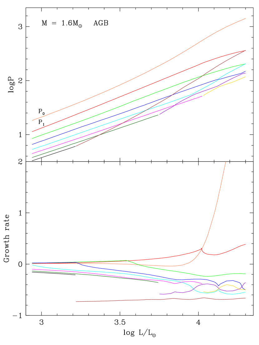
Figure 1: The periods (top panel) and growth rates (bottom panel) for the first 8 radial modes in a series of AGB models with $M=1.6\,{\rm M}_{\odot}$ plotted against luminosity. The growth rate is defined as $exp(-\omega_{\rm i}P)-1$ and it is the fractional growth in amplitude per period ($\omega_{\rm i}$ is the imaginary part of the complex eigenvalue $\omega$). A given mode is defined by its colour with the modal colour being the same in both panels. See the online version for the colours.

Figure 1 shows the period and growth rate for the first 8 radial pulsation modes in a star with $M=1.6\,{\rm M}_{\odot}$ as the luminosity is varied. The optical depth to the centre of the outer zone is set to $\log\tau_{\rm c}=-3$. The maximum luminosity examined for these models with metallicity Z=0.008 is $\log L/{\rm L}_{\odot}=4.3$. This is somewhat larger than the maximum observed luminosity of $\log L/{\rm L}_{\odot}\approx 4$ for stars with $M\approx 1.6\,{\rm M}_{\odot}$ and metallicity ${\rm Z}\approx 0.008$ in the the Magellanic Clouds (Kamath et al., 2010).

At the lowest luminosities ($\log L/L_{\odot}<3.2$), the periods and growth rates of all modes behave smoothly as the luminosity changes. These modes correspond to the normal modes of radial pulsation. We refer to the normal fundamental mode as $P_{0}$, the normal first overtone as $P_{1}$, the normal second overtone as $P_{2}$ and so on. As the luminosity increases past $\log L/{\rm L}_{\odot}\approx 3.2$, a mode appears with a period equal to that of $P_{7}$. The damping rate of this new mode is much higher than that of the normal mode so that the complex eigenvalues $\omega$ of the two modes are very different. As the luminosity of the star increases, the period of the new mode increases more rapidly than that of the normal modes so that the period of the new mode successively equals that of $P_{6}$, $P_{5}$, $P_{4}$, $P_{3}$, $P_{2}$ and $P_{1}$. However, in each case of period equality, the growth rates and hence complex eigenvalues of the two modes are different.

The new mode belongs to the group of modes known as strange modes. Their behaviour is explained lucidly in the paper by Buchler et al. (1997) who show that the strange modes are essentially surface modes with low interior amplitudes. Figure 2 shows the amplitude as a function of radius for a normal and strange mode of identical period (these two modes have $\log L/{\rm L}_{\odot}=4.03$ and they lie at the position where the brown and green lines cross in Figure 1). It can be seen that the strange mode is indeed more concentrated to the stellar surface than the normal mode. In their analysis, Buchler et al. (1997) claimed that the periods of normal modes and a strange modes always avoided crossing but we see no need for this since the eigenvalues of both modes move continuously around the complex $\omega$ plane as separate quantities.

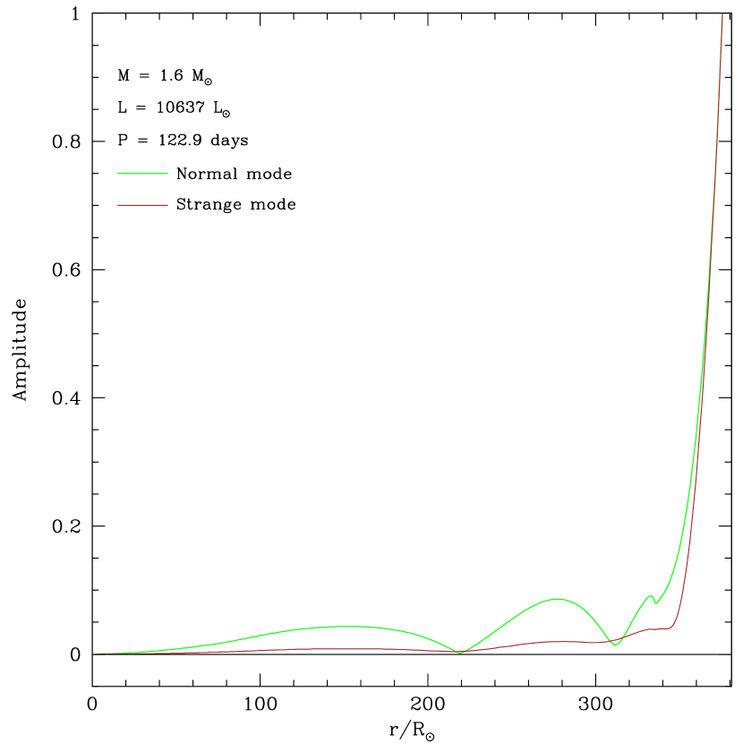
Figure 2: The amplitude of the radius perturbation eigenfunctions for a normal and strange mode of identical period plotted against the radius $r$. The amplitude is $(\delta_{\rm r}^{2}+\delta_{\rm i}^{2})^{\frac{1}{2}}$ where $\delta_{\rm r}$ and $\delta_{\rm i}$ are the real and imaginary parts of radius perturbation $\delta$, respectively. For nonadiabatic pulsation, the amplitude is not necessarily zero at a node. The bump in the curves at $r=335\,{\rm R}_{\odot}$ is caused by the hydrogen ionization zone.

However, avoided crossings do occur. Following $P_{4}$ (the cyan line) from low luminosities in Figure 1, we see that near $\log L/{\rm L}_{\odot}=3.97$ the normal mode $P_{4}$ comes close in period to a second strange mode (purple line). In this case, the two lines avoid crossing in period but they do cross in growth rate. The effect of this is to convert the normal mode into a strange mode and vica versa. In fact, as the luminosity increases further, the mode shown by the purple line undergoes another avoided crossing and converts back from normal mode characteristics to strange mode characteristics. At this time, this strange mode is the third strange mode at these luminosities (where we order the strange modes by decreasing period).

There are also intermediate cases where strange and normal mode periods do cross while at the same time the growth rates are influenced by the other mode. The growth rates tend to be attracted to each other by mode interaction. Examples of this behaviour are the pink and purple modes that cross in period at $\log L/{\rm L}_{\odot}\approx 3.85$ and the blue and cyan modes that cross in period at $\log L/{\rm L}_{\odot}\approx 4.12$. We note that at the high luminosity end of the sequence of $1.6\,{\rm M}_{\odot}$ models, there seems to be a strict alternation between normal and strange modes as one moves to shorter periods. This behaviour does not seem to apply strictly at lower luminosities.

We have found no cases where strange modes have positive growth rates. In fact, Figure 1 shows that the strange modes are always more highly damped than the normal modes. Thus, when considering self-excited modes, we should only expect to see the normal modes of oscillation in real stars. The strange modes may, however, influence both the growth rate and period of normal modes in the case of near-resonance.

It is possible that the strange modes could be stochastically excited by convective motions and thus become observable as part of the solar-like oscillation spectrum which has been detected in red giants at lower luminosity (e.g. Bedding et al., 2010). The peak power of a strange mode in a solar-like oscillation power spectrum will be determined largely by the way in which the convective perturbations can couple to the mode in question. In addition, the peak power will decrease as the damping of the mode increases.

An estimation of the relative amplitudes of stochastically excited normal and strange modes is beyond the scope of this paper. We note that the results in Bányai et al. (2013) show that modes in red giants which have periods $P>10$ days have relatively large amplitudes, which suggests that these modes are self-excitated. On the other hand, the shorter period, lower amplitude modes appear to be stochastically excited. Thus in the luminous red giants considered here, which have $P>10$ days for at least the first two modes, it may be difficult to find the signal of a very damped strange mode in the overall power spectrum where excited modes are likely to dominate. However, if the signal of a strange mode could be detected in a given star, its strange mode nature could possibly be determined by its frequency spacing relative to nearby radial ($\ell=0$) modes.

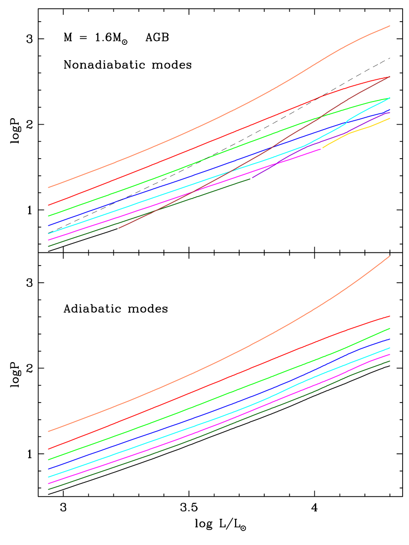
Figure 3: Top panel: Similar to the top panel in Figure 1 but also showing the acoustic cutoff period corresponding to the acoustic cutoff frequency $\sigma_{\rm ac}$ at the surface of the star (dashed black line). Bottom panel: The periods of the first 8 adiabatic radial modes.

Although strange modes and normal modes can have equal periods in the nonadiabatic case, for adiabatic pulsation the Sturm-Liouville theorem requires that the eigenvalues $\omega$ remain distinct. This is shown in Figure 3. However, strange mode behaviour still influences the periods to some extent as seen most prominently for $P_{2}$ and $P_{3}$ (the green and blue modes) near $\log L/{\rm L}_{\odot}\approx 4.15$. A full discussion of the origin of strange mode behaviour in the adiabatic case in given in Buchler et al. (1997).

3.2 The effect of the position of the outer boundary

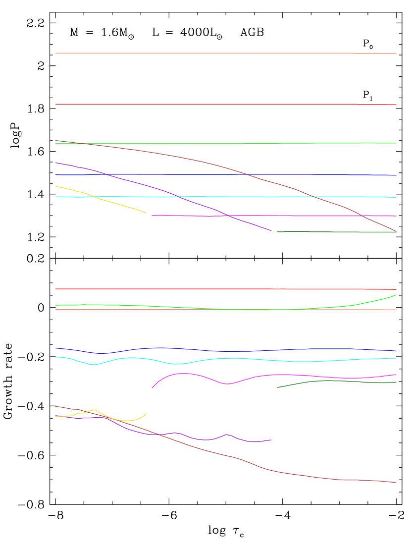
Figure 4: Similar to Figure 1 except that all models have $L=4000\,{\rm L}_{\odot}$ and the periods and growth rates are plotted against $\log\tau_{\rm c}$ rather than $\log L/{\rm L}_{\odot}$.

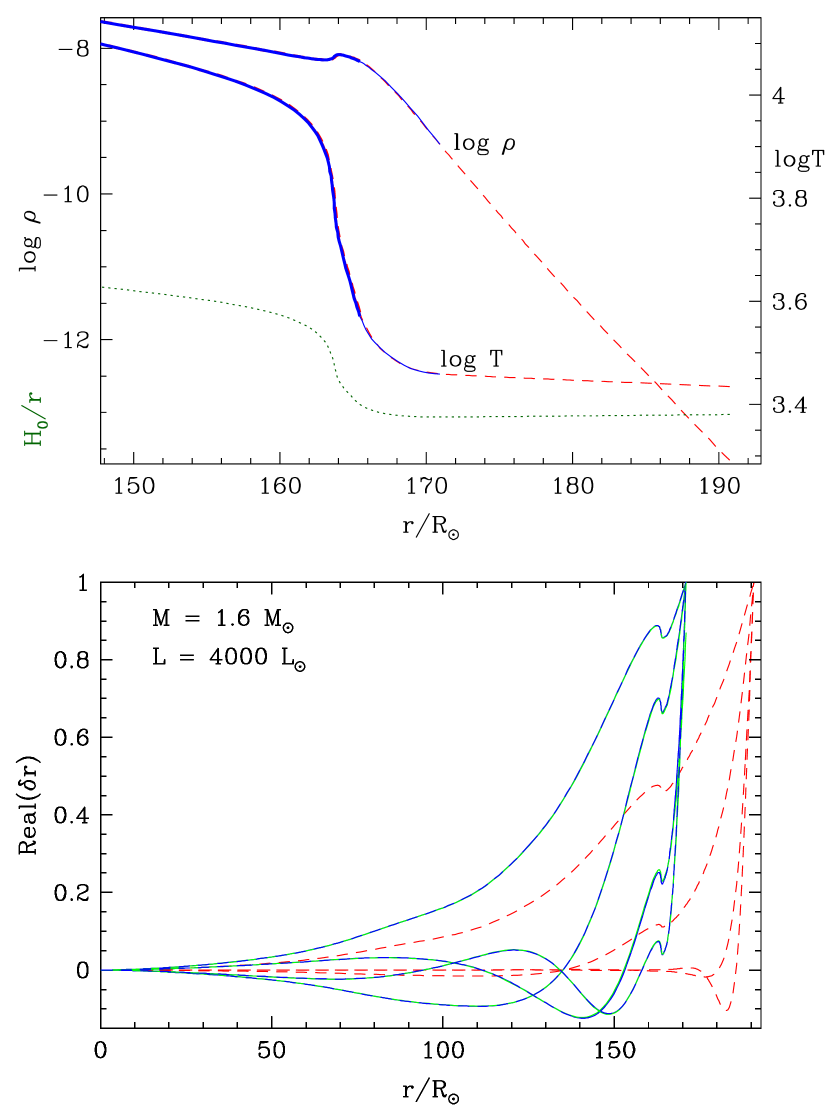
Figure 5: Surface structure and eigenfunctions for models with $M=1.6\,{\rm M}_{\odot}$ and $L=4000\,{\rm L}_{\odot}$. Top panel: $\log\rho$ and $\log T$ plotted against $r$/R_⊙ for a model with $\log\tau_{\rm c}=-3$ (solid blue lines) and a model with $\log\tau_{\rm c}=-8$ (dashed red lines). The thick parts of the line correspond to regions that are convective. The green dotted line shows the ratio of the pressure scale height H₀ to $r$, with a vertical axis scale from 0 to 1. Bottom panel: the real part of the radius eigenfunctions for the first 4 modes of pulsation plotted against the radius $r$. Blue solid lines show the eigenfunctions for the model with $\log\tau_{\rm c}=-3$ while the red dashed lines show the eigenfunctions for the model with $\log\tau_{\rm c}=-8$. These complex eigenfunctions are normalized to 1.0 at the surface for both models. The green dashed lines show the eigenfunctions for the model with $\log\tau_{\rm c}=-8$ normalized to 1.0 at a radius which corresponds to the surface of the model with $\log\tau_{\rm c}=-3$.

We now show how the placement of the outer boundary influences the pulsation periods of red giants. The periods of the eight lowest order modes in a star with $M=1.6\,{\rm M}_{\odot}$ and $L=4000\,{\rm L}_{\odot}$ are plotted against $\log\tau_{\rm c}$ in the Figure 4. Note that a decrease in $\tau_{\rm c}$ means that the surface radius is placed further out in the stellar atmosphere (see below). We restricted $\log\tau_{\rm c}<-2$ since for larger values of $\tau_{\rm c}$ the outer boundary is placed in a region where the temperature gradient starts to become significant and the periods of all modes become dependent of $\tau_{\rm c}$.

It is clear that the periods of the normal modes are independent of $\log\tau_{\rm c}$ i.e. they are independent of the placement of the stellar surface. For the strange modes, the periods vary markedly with $\log\tau_{\rm c}$. This is consistent with the fact that the strange modes are predominantly surface modes largely confined to the region between the hydrogen ionization zone and the stellar surface (Buchler et al., 1997; Saio et al., 1998). The reason that the periods of the strange modes increase as the outer boundary is placed at larger radii is that the ratio $z_{0}$ of the radius of the hydrogen ionization zone to the stellar surface decreases. As shown in the toy models of Buchler et al. (1997) (see their Figure 13), decreasing $z_{0}$ causes the strange mode period to increase relative to the normal mode periods. Note also that it is the decrease in $z_{0}$ with luminosity in the sequence of 1.6 M_⊙ models shown in Figure 1 that causes the strange mode periods to increase faster with luminosity than the normal mode periods.

The strange modes in Figure 4 all have lower growth rates (larger damping rates) than the normal modes. They also cross the periods of the normal modes and in each case it can be seen that mode interaction influences the growth rate as the modes come in and out of resonance.

The top panel of Figure 5 shows the outer structure of a typical luminous red giant from the centre to the surface for two placements of the outer boundary, corresponding to $\log\tau_{\rm c}=-3$ and $\log\tau_{\rm c}=-8$. The model with $\log\tau_{\rm c}=-8$ has a considerably larger surface radius than the model with $\log\tau_{\rm c}=-3$. The physical structure of the two models is essentially indistinguishable at common radii.

The eigenfunctions of the radius perturbation for the 4 lowest order modes are shown in the bottom panel of Figure 5 for the two placements of the outer boundary. At first sight, the eigenfunctions of the corresponding modes in the two models with different surface radii look very different. However, this is not so. To compare the eigenfunctions with the same normalization, the eigenfunctions for the more extended model were multiplied by a complex constant which caused the eigenfunction to be normalized to a value of 1.0 at a radius corresponding to the surface radius of the smaller model. These transformed eigenfunctions are shown as green dashed lines in Figure 5. It can be seen that these transformed eigenfunctions are essentially indistinguishable from those of the less extended model (blue lines) at common radii.

It is not clear to us where the outer boundary should be placed. Clearly, it should be at $\log\tau_{\rm c}<-2$ since the periods of all modes are affected if the outermost model point is deeper in the star than the surface point of the model with $\log\tau_{\rm c}=-2$. Since the periods of the normal modes are essentially independent of the position adopted for the stellar surface, we have adopted $\log\tau_{\rm c}=-3$ as the criterion by which our outer boundary is defined. This value of $\tau_{\rm c}$ also means that the growth rates of the normal modes are not greatly affected by mode interaction with strange modes. As seen in Figure 4, these interactions can become significant for very small $\tau_{\rm c}$ values when the eigenfunctions extend high into the stellar atmosphere.

The strong dependence of strange mode periods on the adopted surface radius means that if strange modes could be detected in the spectrum of solar-like oscillations in a red giant, then the detected periods could be used to determine the outer radius of the red giant as experienced by strange modes.

4 Summary and conclusions

We have shown that in luminous red giant stars, a series of radial strange modes exists in addition to the series of radial normal modes of pulsation. At high luminosities, strange modes can have periods as long as that of the first overtone for plausible luminosities, especially if an extended outer atmosphere in included in the calculations. The periods of the strange modes increase faster with $\log L/{\rm L}_{\odot}$ (and hence surface radius) than the periods of the normal modes. This means that normal and strange modes in a given star can have identical periods at certain luminosities. In some cases, avoided crossings in period occur leading to a given mode (identified by continuity as the luminosity is varied) changing back and forth between a normal and strange mode character as the luminosity changes. In cases where the modes cross in period, the growth rates of each mode is affected by the near-resonance condition. The strange modes are always damped, and more so than the normal modes. We should not expect to see self-excited strange modes in real stars but strange modes may be observed in the spectrum of solar-like oscillations. The periods and growth rates of normal modes may be influened by resonances with strange modes. Fortunately, the normal modes periods are essentially unaffected by the placement of the outer boundary. On the other hand, the strange mode periods increase as the outer boundary is placed at larger radii. Finally, we note that although these calculations were performed for radial modes, we expect that strange modes should also exist in the nonradial case.

References

- Baker & Kippenhahn (1965) Baker N., Kippenhahn R., 1965, ApJ, 142, 868
- Bányai et al. (2013) Bányai E., et al., 2013, MNRAS, 436, 1576
- Bedding et al. (2010) Bedding T. R., et al., 2010, ApJ, 713, L176
- Bertelli et al. (2008) Bertelli G., Girardi L., Marigo P., Nasi E., 2008, A&A, 484, 815
- Buchler et al. (1997) Buchler J. R., Yecko P. A., Kollath Z., 1997, A&A, 326, 669
- Buchler & Kollath (2001) Buchler J. R., Kollath Z., 2001, ApJ, 555, 961
- Fox & Wood (1982) Fox M. W., Wood P. R., 1982, ApJ, 259, 198
- Fraser et al. (2005) Fraser O. J., Hawley S. L., Cook K. H., Keller S. C., 2005, AJ, 129, 768
- Iglesias & Rogers (1996) Iglesias C. A., Rogers F. J., 1996, ApJ, 464, 943
- Ita et al. (2004) Ita Y., et al., 2004, MNRAS, 347, 720
- Kamath et al. (2010) Kamath D., Wood P. R., Soszyński I., Lebzelter T., 2010, MNRAS, 408, 522
- Keller & Wood (2006) Keller, S. C., Wood, P. R., 2006, ApJ, 642, 834
- Marigo & Aringer (2009) Marigo P., Aringer B., 2009, A&A, 508, 1539
- Saio et al. (1998) Saio H., Baker N. H., Gautschy A., 1998, MNRAS, 294, 622
- Soszynski et al. (2007) Soszynski I., et al., 2007, AcA, 57, 201
- Takayama, Saio & Ita (2013) Takayama M., Saio H., Ita Y., 2013, MNRAS, 431, 3189
- Wood et al. (1999) Wood P. R., et al., 1999, IAUS, 191, 151
- Wood & Zarro (1981) Wood P. R., Zarro D. M., 1981, ApJ, 247, 247