SE-106 91 Stockholm, Swedenddinstitutetext: Bethe Center for Theoretical Physics, Bonn University, Germanyeeinstitutetext: Deutsches Elektronen-Synchrotron DESY, Notkestraße 85, D-22607 Hamburg, Germany
Probing the Standard Model with Higgs signal rates from the Tevatron, the LHC and a future ILC
Abstract
We explore the room for possible deviations from the Standard Model (SM) Higgs boson coupling structure in a systematic study of Higgs coupling scale factor () benchmark scenarios using the latest signal rate measurements from the Tevatron and LHC experiments. We employ fits performed with HiggsSignals, which takes into account detailed information on signal efficiencies and major correlations of theoretical and experimental uncertainties. All considered scenarios allow for additional non-standard Higgs boson decay modes, and various assumptions for constraining the total decay width are discussed. No significant deviations from the SM Higgs boson coupling structure are found in any of the investigated benchmark scenarios. We derive upper limits on an additional (undetectable) Higgs decay mode under the assumption that the Higgs couplings to weak gauge bosons do not exceed the SM prediction. We furthermore discuss the capabilities of future facilities for probing deviations from the SM Higgs couplings, comparing the high luminosity upgrade of the LHC with a future International Linear Collider (ILC), where for the latter various energy and luminosity scenarios are considered. At the ILC model-independent measurements of the coupling structure can be performed, and we provide estimates of the precision that can be achieved.
Keywords:
Higgs Physics, Beyond Standard Model1 Introduction
On July 4, 2012 the discovery of a narrow resonance, with a mass near , in the search for the Standard Model (SM) Higgs boson at the Large Hadron Collider (LHC) was announced at CERN by both the ATLAS and CMS experiments Aad:2012tfa ; Chatrchyan:2012ufa . The initial discovery was based on the data collected at the LHC until June 2012, and these results have since been confirmed and refined using the full 2012 data set ATLAS:2013sla ; ATLAS:2013mla ; CMS:yva ; CMS:2013wda . Results from the Tevatron experiments Aaltonen:2013kxa support the findings. Within the current experimental and theoretical uncertainties the properties of the newly discovered particle are thus far in very good agreement with the predictions for a SM Higgs boson, including the measurements of signal rates as well as further properties such as spin.
In order to test the compatibility of the newly observed boson with the predictions for the Higgs boson of the SM based on the data accumulated up to 2012, the LHC Higgs Cross Section Working Group (LHCHXSWG) proposed several benchmark scenarios within an “interim framework” employing Higgs coupling scale factors LHCHiggsCrossSectionWorkingGroup:2012nn ; Heinemeyer:2013tqa . This approach is based on earlier studies of the LHC sensitivity to Higgs couplings initiated in Refs. Zeppenfeld:2000td ; Duhrssen:2003tba ; Duhrssen:2004cv ; Duhrssen:2004uu and has been influenced by further analyses as described in Refs. LHCHiggsCrossSectionWorkingGroup:2012nn ; Heinemeyer:2013tqa , see also Ref. LHCHiggsCrossSectionWorkingGroup:2012nn concerning the discussion of a more general framework based on suitable effective Lagrangians. The coupling scale factors have been analyzed by the experimental collaborations ATLAS:2013sla ; CMS:yva as well as in further phenomenological studies where Higgs coupling fits have been carried out Lafaye:2009vr ; Klute:2012pu ; Plehn:2012iz ; Klute:2013cx ; Dobrescu:2012td ; Espinosa:2012im ; Cacciapaglia:2012wb ; Belanger:2012gc ; Ellis:2013lra ; Djouadi:2013qya ; Cheung:2013kla ; Holdom:2013axa ; Chpoi:2013wga ; Bechtle:2013xfa ; Belanger:2013xza . The results of those analyses show no significant deviations from SM Higgs couplings.
The total Higgs decay width for a Higgs boson mass around is not expected to be directly observable at the LHC. In the SM, a total width around is predicted, which is several orders of magnitude smaller than the experimental mass resolution. Suggestions to achieve more sensitive constraints on the total width other than the ones limited by the experimental mass resolution have been made. These are based on the analysis of off-shell contributions from above the Higgs resonance in Higgs decays to or final states Caola:2013yja ; Campbell:2011cu ; Campbell:2013wga ; Campbell:2013una and of interference effects between the signal and the background continuum Dixon:2013haa . However, the ultimate sensitivities are expected to remain about one order of magnitude above the level of the SM width. The limited access of the LHC to the Higgs width implies that only ratios of couplings can be determined at the LHC, rather than couplings themselves, unless additional theory assumptions are made.
Looking beyond the SM, a generic property of many theories with extended Higgs sectors is that the lightest scalar can have nearly identical properties to the SM Higgs boson. In this so-called decoupling limit, additional states of the Higgs sector are heavy and may be difficult to detect in collider searches. Deviations from the Higgs properties in the SM can arise from an extended structure of the Higgs sector, for instance if there is more than one Higgs doublet. Another source of possible deviations from the SM Higgs properties are loop effects from new particles. The potential for deciphering the physics of electroweak symmetry breaking is directly related to the sensitivity for observing deviations from the SM. Given the far-reaching consequences for our understanding of the fundamental structure of matter and the basic laws of nature, it is of the highest priority to probe the properties of the newly discovered particle with a comprehensive set of high-precision measurements. In particular, the determination of its couplings to other particles with the highest possible precision is crucial.
The aim of this paper is to investigate whether there are hints of deviations from the SM Higgs couplings based on a combined picture of all the latest results from the Tevatron and LHC experiments. By investigating a complete selection of possible scale factor parametrizations of Higgs coupling strengths ranging from highly constrained to very generic parametrizations, we systematically study potential tendencies in the signal rates and correlations among the fit parameters. In all considered scenarios we allow for additional Higgs decay modes that are either assumed to be altogether invisible Higgs decay modes, thus yielding a missing energy collider signature, or considered to be undetectable decay modes. In the latter case, additional model assumptions have to be imposed to constrain the total width at the LHC. Based on those assumptions an upper limit on the branching ratio of the undetectable decay mode can be derived for each parametrization.
Going beyond the present status, we analyze the prospects of Higgs coupling determination at future LHC runs with and of integrated luminosity, as well as with a future International Linear Collider (ILC). The estimated ILC capabilities are presented both for a model-dependent and model-independent fit framework. In the first case, the total width is constrained by imposing the same assumptions as required for the LHC, and we compare the ILC capabilities directly with those of the high-luminosity LHC (HL–LHC) with . In the latter case, the total width is only constrained by the total cross section measurement of the process at the ILC, thus enabling measurements of coupling scale factors free from theoretical prejudice.
Finding significant deviations in any Higgs coupling scale factors would provide a strong motivation for studying full models which exhibit a corresponding coupling pattern. However, the fit results obtained within the framework of coupling scale factors can in general not be directly translated into realistic new physics models, see Sect. 2.1 for a discussion. Concerning the investigation of particular models of new physics, the most reliable and complete results are obtained by performing a dedicated fit of the Higgs signal rates within the considered model. Such model-dependent fits, see e.g. Buckley:2012em ; Arbey:2012na ; Arbey:2012dq ; Akula:2012kk ; Cao:2012yn ; Howe:2012xe ; Drees:2012fb ; Haisch:2012re ; Bechtle:2012jw ; Arbey:2012bp ; Ke:2012zq ; Chakraborty:2013si ; Carmona:2013cq ; Arbey:2013jla ; Cao:2013wqa ; Bhattacherjee:2013vga ; Lopez-Val:2013yba ; Belyaev:2013ida ; Cao:2013gba ; Bharucha:2013ela ; Cheung:2013rva ; Bechtle:2013mda ; Cao:2013mqa ; Djouadi:2013lra ; Enberg:2013jba ; Cao:2013cfa ; Wang:2013sha ; Fan:2014txa ; Belanger:2014roa ; Stal:2014sua for recent studies, can easily be performed with the generic code HiggsSignals Bechtle:2013xfa ; Stal:2013hwa that has been used to perform this work.
This paper is organized as follows. Sect. 2 introduces the fit methodology and the statistical treatment employed in HiggsSignals. This section also contains a discussion of the experimental input and and the treatment of theoretical uncertainties, with further details given in the Appendix. In Sect. 3 we present the fit results for the various benchmark parametrizations of Higgs coupling scale factors using all the currently available data from the LHC and the Tevatron. Results for future expectations are presented in Sect. 4. Here the current data is replaced by the projections for the future precision at the HL–LHC and the ILC, and we discuss the accuracy to which the Higgs coupling scale factors can be determined in the various scenarios. The conclusions are given in Sect. 5. Additional information can be found in the three appendices. Appendix A presents the experimental dataset that is used (and its validation). Appendix B contains a discussion of the statistical -value derived from tests of model predictions against measurements of Higgs boson signal rates. Finally, Appendix C contains further details on how we treat the theoretical uncertainties of Higgs production and decay rates.
2 Methodology
2.1 Coupling scale factors
The SM predicts the couplings of the Higgs boson to all other known particles. These couplings directly influence the rates and kinematic properties of the production and decay of the Higgs boson. Therefore, measurements of the production and decay rates of the observed state, as well as their angular correlations, yield information that can be used to probe whether data is compatible with the SM predictions.
In the SM, once the numerical value of the Higgs mass is specified, all the couplings of the Higgs boson to fermions, gauge bosons and to itself are specified within the model. It is therefore in general not possible to perform a fit to experimental data within the context of the SM where Higgs couplings are treated as free parameters Cornwall:1973tb ; LlewellynSmith:1973ey . In order to test the compatibility of the newly observed boson with the predictions for the SM Higgs boson and potentially to find evidence for deviations in the 2012 data, the LHC Higgs Cross Section Working Group (LHCHXSWG) proposed several benchmark scenarios containing Higgs coupling scale factors within an “interim framework” LHCHiggsCrossSectionWorkingGroup:2012nn ; Heinemeyer:2013tqa . This framework is based on several assumptions. In particular, all deviations from the SM are computed assuming that there is only one underlying state at . It is assumed that this state is a Higgs boson, and that it is SM-like, in the sense that the experimental results so far are compatible with the SM Higgs boson hypothesis. Also the coupling tensor structures are assumed to be as in the SM, meaning in particular that the state is CP-even scalar. Furthermore, the zero width approximation is assumed to be valid, allowing for a clear separation and simple handling of production and decay of the Higgs particle.
In order to take into account the currently best available SM predictions for Higgs cross sections and partial widths, which include higher-order QCD and EW corrections Dittmaier:2011ti ; Dittmaier:2012vm ; Heinemeyer:2013tqa , while at the same time introducing possible deviations from the SM values of the couplings, the predicted SM Higgs cross sections and partial decay widths are dressed with scale factors . The scale factors are defined in such a way that the cross sections or the partial decay widths associated with the SM particle scale with the factor when compared to the corresponding SM prediction.111Note, that in this interim framework, slight dependencies of the derived collider observables (cross sections , partial widths ) on the remaining Higgs coupling scale factors, , are often neglected. For instance, the cross section of the Higgs-strahlung process features a small dependence on the top-Yukawa coupling scale factor entering via the NNLO process Harlander:2013mla . However, for scale factor ranges, , this effect is negligible. Hence, the cross section can be simply rescaled by . The most relevant coupling scale factors are , , , , , …In the various benchmark scenarios defined in Ref. LHCHiggsCrossSectionWorkingGroup:2012nn ; Heinemeyer:2013tqa several assumptions are made on the relations of these scale factors in order to investigate certain aspects of the Higgs boson couplings, as will be discussed here in Sect. 3.
One should keep in mind that the inherent simplifications in the framework make it rarely possible to directly map the obtained results onto realistic models beyond the SM (BSM). The scale factor benchmark scenarios typically have more freedom to adjust the predicted signal rates to the measurements than realistic, renormalizable models. The latter generally feature specific correlations among the predicted rates, which furthermore can depend non-trivially and non-linearly on the model parameters. Moreover, constraints from the electroweak precision data and possibly other sectors, such as dark matter, collider searches, vacuum stability, etc., can further restrict the allowed parameter space and thus the room for Higgs coupling deviations. Preferred values and confidence regions of the scale factors obtained from profiling over regions in the parameter space, which are not covered by the allowed parameter space of the full model, cannot be transferred to the full model. The implications of the Higgs signal rate measurements for the full model can then only be investigated consistently in a dedicated, model-dependent analysis. In that sense, such analyses of realistic BSM models are complementary to the approach followed here, and can easily be performed with the same tools and statistical methods as employed here.
One limitation at the LHC, but not at the ILC, is the fact that the total width cannot be determined experimentally without additional theory assumptions. In the absence of a total width measurement only ratios of ’s can be determined from experimental data. In order to go beyond the measurement of ratios of coupling scale factors to the determination of absolute coupling scale factors additional assumptions are necessary to remove one degree of freedom. One possible and simple assumption is that there are no new Higgs decay modes besides those with SM particles in the final state. Another possibility is to assume the final state of potentially present additional Higgs decay(s) to be purely invisible, leading to a boson recoiling against missing transverse energy in the Higgs-strahlung process at the LHC Eboli:2000ze . By employing constraints from dedicated LHC searches for this signature the total width can be constrained. In both cases, further assumptions need to be imposed on the partial widths of Higgs decays to SM particles which are unobservable at the LHC, like for instance . As a third possibility, an assumption can be made on the couplings of the Higgs to the SM gauge bosons, Duhrssen:2004cv ; Duhrssen:2004uu . This assumption is theoretically well-motivated as it holds in a wide class of models. For instance, they hold in any model with an arbitrary number of Higgs doublets, with and without additional Higgs singlets, or in certain classes of composite Higgs models. We will partly make use of these assumptions in our analysis below. More details will be given in Sect. 3.
2.2 The statistical analysis using HiggsSignals
We use the public computer program HiggsSignals Bechtle:2013xfa ; Stal:2013hwa , based on the HiggsBounds-4 library Bechtle:2008jh ; Bechtle:2011sb ; Bechtle:2013gu ; Bechtle:2013wla , which is a dedicated tool to test model predictions of arbitrary Higgs sectors against the mass and signal rate measurements from Higgs searches at the LHC and the Tevatron. For both types of measurement a statistical value can be evaluated, denoted as for the signal rates and for the Higgs mass. In this work we are only interested in the contribution from the signal rates and fix the Higgs mass to .
The Higgs signal rate measurement performed in an analysis , denoted by , is given by the experiments as a SM normalized quantity. It contains all relevant Higgs collider processes, where each process is comprised of a production mode and a decay mode , and features a specific efficiency . The observed signal strength modifier can thus be understood as a universal scale factor for the SM predicted signal rates of all involved Higgs processes. The corresponding model-predicted signal rates are calculated as
| (1) |
In general, the efficiencies can be different from the SM for models where the influence of Higgs boson interaction terms with a non-standard (higher-dimensional or CP-odd) tensor-structure cannot be neglected Banerjee:2013apa ; Anderson:2013afp ; Azatov:2013xha ; Boos:2013mqa ; Chen:2013waa ; Buchalla:2013mpa ; Dumont:2013wma . In this paper, the efficiencies are assumed to be identical for the SM and the unknown model predicting the rescaled signal rates. This assumption is valid for small deviations from the SM Higgs couplings, where kinematic effects changing the efficiencies can be neglected. However, if significant deviations from the SM are found from the analysis, a more careful investigation of anomalous Higgs couplings Buchmuller:1985jz ; Contino:2013kra ; Pomarol:2013zra becomes necessary, including a detailed study of their effects on the efficiencies. On the experimental side, the publication of differential fiducial cross sections should then be considered Boudjema:2013qla .
In this work we employ hybrid Bayesian-frequentist fits based on the value derived from HiggsSignals. In this approach the systematic uncertainties are parametrized using Gaussian probability density functions, while all model parameters are treated in a frequentist manner. In order to determine the uncertainties on individual model parameters in multi-dimensional fits we profile over the remaining model parameters. A “naive” -value, i.e. the probability of falsely rejecting a specific model assuming it is true, is quoted based on the agreement between the minimal value found in the fit and the number of degrees of freedom (ndf). However, the value evaluated by HiggsSignals does not generically fulfill the prerequisite for this simple -value estimation: Firstly, HiggsSignals uses asymmetric uncertainties in order to take into account remaining non-Gaussian effects in the measurements. Secondly, the signal rate uncertainties are comprised of constant and relative parts. The latter include the theoretical uncertainties on the cross sections and branching ratios, which are proportional to the signal rate prediction, as well as the luminosity uncertainty, which is proportional to the measured signal rate. These features are necessary in order to effectively reproduce the properties of the full likelihood implementation as done by the experimental collaborations and ensure the correct scaling behavior when testing models different from the SM Bechtle:2013xfa .
These features potentially introduce deviations from the naive behavior, which could affect both the extraction of preferred parameter ranges at a certain confidence level (C.L.) as well as the calculation of the -value. In order to estimate the impact of these effects, we performed a Monte Carlo (MC) toy study for a simple one-dimensional scale factor model, which is presented in Appendix B. From this study two important conclusions can be drawn: Firstly, the central value and uncertainties of the estimated fit parameter extracted from the full toy study do indicate a small variation from the naive values extracted from profiling. However, these variations are each less than . Hence, we are confident that the uncertainties and best fit values quoted later for the profile likelihood scans are valid to a good approximation. Secondly, the -value obtained in the full MC toy study can be different to the naive distribution. For an example of a change in the shape of the observed probability density function in toy experiments, see Fig. 23 in Appendix B, which indicates that the actual -value may be higher than expected when assuming an ideal distribution. This effect could be significant and should be taken into account once this technique is used to exclude models, e.g. once the probability comes close to 5%. As will be discussed later in this work, we find naive -values for the best-fit points of all considered models in the range of 25 – 35%, which are far away from any critical border. Therefore, we are confident that the conclusions drawn from the naive -values in the remainder of the paper would not change in any significant way if a full toy study or, even better, a full likelihood analysis by the experimental collaborations, was done for every fit.
Within HiggsSignals the correlations of theoretical cross section, branching ratio and luminosity uncertainties among different observables are taken into account Bechtle:2013xfa . For this work, we further develop this implementation to also take into account major correlations of experimental systematic uncertainties for a few important analyses where the necessary information is provided. Specifically, this is the case for the CMS analysis CMS:ril and the ATLAS analysis ATLAS-CONF-2013-108 . More details are given in Sect. 2.3 and Appendix A, including a comparison with official results.
We want to note that an alternative approach for transferring the experimental results into global Higgs coupling or model fits exists Belanger:2013xza ; Boudjema:2013qla . This approach suggests that the experiments provide combined higher-dimensional likelihood distributions for scale factors of the Higgs boson production modes. On first sight, an appealing feature is that correlations among the combined analyses of the experimental and theoretical uncertainties for the model investigated by the analysis (usually the SM) are automatically taken care of by the collaborations. However, when going beyond the combination of that specific selection of analyses, e.g. when combining ATLAS and CMS results, or already when combining the likelihoods of different decay modes, detailed knowledge of the correlations of common uncertainty sources is again required. Moreover, a careful treatment of these correlations in a combination, as is done for the simple one-dimensional signal strength measurements in HiggsSignals, is far more complicated for higher-dimensional likelihoods. We therefore advise the collaborations to continue providing one-dimensional signal strength measurements, including detailed information on signal efficiencies and correlations, since then the amount of model-dependence in the experimental results is rather minimal CorrSystDoc . Nevertheless, we also support the suggestions made in Refs. Boudjema:2013qla , since these higher-dimensional likelihoods are still useful on their own and for validation. Note also recently proposed attempts to disentangle theoretical uncertainties from signal strength measurements Cranmer:2013hia .
The technical details of the profiled likelihood scans performed in this work are as follows. For an efficient sampling of the parameter space the scans are performed with an adaptive Metropolis (AM) algorithm haario2001ama with flat prior probability distributions using the Markov-Chain Monte Carlo (MCMC) python package PyMC Patil:Huard:Fonnesbeck:2010 . Appropriate initial values for the MCMC chains are found using the maximum a posteriori estimate (MAP) class of PyMC. The scans contain around – points, depending on the dimensionality of the parameter space. For each scan, several Markov chains are run independently of each other, featuring a typical length of scan points. The results are presented in a purely frequentist’s interpretation based on the global derived from HiggsSignals and, optionally, further contributions arising from constraints from invisible Higgs searches at the LHC. Hence, the Markov Chains merely serve as a sampling method of the parameter space and no Bayesian interpretation is employed. This resulting higher-dimensional distribution is then profiled in order to obtain one- and two-dimensional likelihoods for the fit parameters and related quantities. The parameter regions around the best-fit point are then obtained for values of the difference to the minimal value, , of for the one-dimensional, and for the two-dimensional profiles, respectively. As discussed above, we also quote for each benchmark scenario the fit quality at the best-fit point, given by , and the corresponding (naively estimated) -value.
2.3 Experimental input from the Tevatron and the LHC
In the analysis of the present status of potential deviations in the Higgs couplings, presented in Sect. 3, we use the latest available signal strength measurements from the Tevatron and LHC experiments, which are included in HiggsSignals-1.2.0. Detailed information on these in total signal strength measurements and the assumed signal composition of the production modes is given in Appendix A. Notably, these measurements include the recently published results from ATLAS in the channel ATLAS-CONF-2013-108 , for which we implement correlations of experimental systematic uncertainties in HiggsSignals, cf. Appendix A. Based on the comparison of a six-dimensional scale factor fit to the official CMS results CMS:yva , we perform an approximate rescaling of the CMS measurements CMS:ril from the published Higgs mass value of to the best-fit combined mass of . Using the rescaled measurements, we find very good agreement with the official CMS fit results, see Appendix A.2 for details.
2.4 Treatment of theoretical uncertainties
We attempt to account for various correlations among the theoretical uncertainties of the cross section and branching ratio predictions. Correlations of theoretical uncertainties among different signal strength observables, as well as correlations among the theoretical uncertainties themselves induced by e.g. common parametric dependencies, are taken into account in HiggsSignals since version 1.1.0 HSreleasenote . Here we outline how the latter type of correlations is evaluated. More details are given in Appendix C.
The contributions of the major parametric and theoretical (higher-order) uncertainty sources to the total uncertainties of the partial decay widths and production cross sections are given separately by the LHCHXSWG in Refs. Denner:2011mq ; Heinemeyer:2013tqa . However, there is unfortunately no consensus on how these contributions can be properly combined since the shapes of the underlying probability distributions are unknown. Hence, thus far, the use of conservative maximum error estimates is recommended. Nevertheless, such a prescription is needed in order to account for the correlations. In this work we employ covariance matrices evaluated by a Monte Carlo (MC) simulation, which combines the parametric and theoretical uncertainties in a correlated way. The importance of a combination prescription for precision Higgs coupling determination in the future ILC era is briefly discussed in Appendix C.
The relative parametric uncertainties (PU) on the partial Higgs decay widths, , from the strong coupling, , and the charm, bottom and top quark mass, , and , respectively, as well as the theoretical uncertainties (THU) from missing higher order corrections, , are given in Tab. 1 of Ref. Heinemeyer:2013tqa . The PUs are given for each decay mode for both positive and negative variation of the parameter. From this response to the parameter variation we can deduce the correlations among the various decay modes resulting from the PUs. More importantly, correlations between the branching ratio uncertainties are introduced by the total decay width, .
The covariance matrix for the Higgs branching ratios is then evaluated with a toy MC: all PUs are smeared by a Gaussian of width , where the derived correlations are taken into account. Similarly, the THUs are smeared by a Gaussian or a uniform distribution within their uncertainties. Hereby, we treat all THUs as uncorrelated, except for those of and production. These are treated as fully correlated due to their common higher-order QCD effects. We find that both probability distributions give approximately the same covariance matrix. A detailed description of our procedure is given in Appendix C, including a comparison of different implementations and assumptions on the theoretical uncertainties in the light of future data from the high luminosity LHC and ILC. Overall, we find slightly smaller estimates for the uncertainties than those advocated by the LHCHXSWG, cf. Appendix C. This is not surprising, since the (very conservative) recommendation is to combine the uncertainties linearly.
Using the present uncertainty estimates Heinemeyer:2013tqa , the correlation matrix for the branching ratios in the basis () is given by
| (2) |
As can be seen, strong correlations are introduced via the total width. As a result, the channel, which dominates the total width, as well as the channel are anti-correlated with the remaining decay modes.
For the production modes at the LHC with a center-of-mass energy of the correlation matrix in the basis (ggH, VBF, , , ) is given by
| (3) |
Significant correlations appear between the gluon fusion (ggH) and production processes due to common uncertainties from the parton distributions and QCD-scale dependencies, as well as among the vector boson fusion (VBF) and associate Higgs-vector boson production (, ) channels.
These correlations are taken into account in all fits presented in this work. The numerical values presented in Eqs. (2) and (3) are evaluated for the setting used in the fits to current measurements, cf. Sect. 3, as well as in the conservative future LHC scenario (S1), see Sect. 4.1. For the other future scenarios discussed in Sect. 4, we re-evaluate the covariance matrices based on the assumptions on future improvements of parametric and theoretical (higher-order) uncertainties. However, while the magnitude of the uncertainties changes in the various scenarios discussed later, we find that the correlations encoded in Eqs. (2) and (3) are rather universal. A comparison of uncertainty estimates among all future scenarios we discuss, as well as with the recommended values from the LHCHXSWG, can be found in Appendix C.
3 Current status of Higgs boson couplings
In this section we explore the room for possible deviations from the SM Higgs boson couplings for various benchmark models, each targeting slightly different aspects of the Higgs sector. We follow the LHCHXSWG interim framework LHCHiggsCrossSectionWorkingGroup:2012nn ; Heinemeyer:2013tqa for probing (small) deviations from the SM Higgs boson couplings by employing simple scale factors for the production and decay rates. Hereby, we assume that the LHC Higgs signal is due to a single narrow resonance with a mass of . The experimental signal efficiencies of the various analyses are assumed to be unchanged with respect to the SM Higgs signal. This corresponds to the underlying assumption that the tensor structure of the couplings is the same as in the SM, i.e. we investigate the coupling structure of a -even, scalar boson.
The LHC signal rate measurements, i.e. measurements of the product of a production cross section times the branching ratio to a certain final state, do not provide direct information about the total width of the Higgs boson. Hence, the LHC is regarded as being insensitive to probe the total Higgs width, , unless it features a very broad resonance, . The current best limit, at , is obtained by CMS using the channel Chatrchyan:2013mxa . An even more recent proposal is to exploit the invariant mass spectrum in the process , where the total Higgs decay width can be constrained due to strongly enhanced contributions from off-shell Higgs production. This has been projected to yield a upper limit of using current data, and a potential future sensitivity of is claimed for increased integrated luminosity Caola:2013yja ; Campbell:2013una . A total width of that order still allows for a significant branching fraction to undetectable/invisible final states and sizable coupling modifications. SM-like signal rates for a Higgs boson with an increased total width can always be obtained by a simultaneous increase of the branching fraction to undetectable particles and the Higgs couplings to SM particles, if both are allowed to vary and no further assumptions are imposed Duhrssen:2004cv ; Duhrssen:2004uu ; Belanger:2013kya .222Although the scale factor framework technically features a perfect degeneracy between an increasing and increasing scale factors of the Higgs couplings to SM particles if no additional constraints are imposed, the validity of the underlying model assumptions — in particular the assumption of identical signal efficiencies as in the SM — need to be scrutinized carefully in parameter regions with significant deviations from the SM Higgs couplings. In general, effects leading to such large coupling deviations within the underlying (unknown) model may potentially also lead to different kinematical distributions and hence to changed signal efficiencies. Furthermore, the narrow width approximation will become worse for an increasing total width. Given the signal rate measurements from the experiments at the Tevatron and the LHC, this degeneracy can only be overcome by additional model assumptions and constraints.
In our analysis, we generally allow for an additional branching fraction to new physics, . Concerning the assumptions needed to constrain the total width, we distinguish the two cases of the additional branching fraction being comprised of either invisible or undetectable Higgs decays. The invisible decays are considered to measurable/detectable via e.g. the Higgs-strahlung process, leading to a boson recoiling against missing transverse energy at the LHC Eboli:2000ze . Invisible Higgs decays can appear in models where the Higgs boson couples to a light dark matter (DM) candidate, as for instance in light singlet DM models Cline:2013gha or supersymmetry with a stable neutralino as the lightest supersymmetric particle (LSP). In contrast, the undetectable decays cannot be constrained by any present LHC analysis. Possible examples are or other light flavored hadronic Higgs decays as these signatures are considered indistinguishable from the background. Other examples can be found in theories beyond the SM, like for instance, decays to supersymmetric particles that further decay via SUSY cascades or via -parity violating interactions Dreiner:1997uz ; Barbier:2004ez , which also potentially leading to detached vertices. In this work we investigate the following two options to overcome this degeneracy:
-
(i)
All additional Higgs decay modes yield an invisible final state, i.e.
(4) Hence, results from ATLAS and CMS searches measuring the recoil of a boson against missing transverse energy in the production can be used to constrain .
-
(ii)
The Higgs-vector boson coupling scale factor is required to be . The Higgs production in the and VBF channels is then constrained from above Duhrssen:2004cv ; Duhrssen:2004uu . In this case, no assumption on additional Higgs decay modes needs to be imposed. Hence, an upper limit on can be derived from the fit result Belanger:2013xza . This assumption is valid for models that contain only singlet and doublet Higgs fields. However, in models with higher Higgs field representations Georgi1985 ; Chanowitz1985 ; Gunion1990 ; oai:arXiv.org:hep-ph/0306034 ; oai:arXiv.org:1202.1532 ; Chang2012 ; Hisano:2013sn ; Kanemura:2013mc this assumption does generally not hold.
As will be discussed in Sect. 4.2, both assumptions become obsolete once the direct cross section measurement for becomes available from the ILC.
In the following Sections 3.1–3.6 we discuss several fits to benchmark parametrizations of Higgs coupling deviations, where we also allow for an additional Higgs boson decay mode leading to an invisible final state (i). In this case, we further constrain the product by adding the profile likelihood, , from the ATLAS search ATLAS:2013pma to the global obtained from HiggsSignals.333CMS carried out similar searches for the process and obtained upper limits corresponding to (for ) CMS:2013yda and (for ) CMS-PAS-HIG-13-028 . However, unlike ATLAS, CMS does not provide a profile likelihood that can be incorporated into our fit. In Sect. 3.7 we instead employ the theoretical constraint (ii) to constrain the total width. Under this condition we derive for each benchmark parametrization upper limits on a new Higgs decay mode, which apply irrespectively of whether the final state is truly invisible or just undetectable.
If the individual scale factors for the loop-induced Higgs couplings to gluons and photons, and , respectively, are not treated as individual free parameters in the fit, they can be derived from the fundamental Higgs coupling scale factors. We generally denote such derived scale factors as . Additional genuine loop contributions from BSM particles to these effective couplings are then assumed to be absent. The Higgs-gluon scale factor is then given in terms of and as LHCHiggsCrossSectionWorkingGroup:2012nn ; Heinemeyer:2013tqa
| (5) |
Here, , and denote the contributions to the cross section from the top-quark loop, the bottom-quark loop and the top-bottom interference, respectively. For a Higgs mass around the interference term is negative for positive scale factors. Details about state-of-the-art calculations have been summarized in Refs. Dittmaier:2011ti ; Dittmaier:2012vm ; Heinemeyer:2013tqa . We use numerical values for the different contributions to Eq. (5) extracted from FeynHiggs-2.9.4 Heinemeyer:1998yj ; Hahn:2009zz for a center-of-mass energy of . These evaluations are based on the calculations presented in Ref. Aglietti:2006tp ; Bonciani:2007ex . The top Yukawa contributions are calculated up to NNLO, whereas the bottom Yukawa contributions are evaluated up to NLO. These calculations agree well with the numbers used so far by the experimental collaborations Dittmaier:2011ti .
Similarly to , the scale factor for the loop-induced Higgs-photon coupling, , is derived from the coupling scale factors and contributions to the partial width of the involved particles in the loop,
| (6) |
where loops over the particles , , , , , ,, , , . The have been evaluated with HDECAY Djouadi:1997yw ; Spira:1997dg . The partial widths are derived by setting , (). Then the cross terms are derived by first calculating with and , and then subtracting and . Despite the absence of a sensitive observable probing the Higgs coupling to directly, we also derive the coupling scale factor in order to infer indirect constraints on this quantity and to evaluate its contribution to the total decay width. This scale factor coupling is derived in complete analogy to .
In the following benchmark fits, we choose to parametrize our results in terms of the absolute scale factors, , and an additional branching ratio to new particles, . These parameters can be transformed into the total width scale factor used in the benchmark model proposals from the LHCHXSWG LHCHiggsCrossSectionWorkingGroup:2012nn ; Heinemeyer:2013tqa ,
| (7) |
where is the derived scale factor for the SM total width as induced by the modified Higgs couplings to SM particles, (both including the fundamental and loop-induced couplings). For an allowed range , the total width scale factor, , thus ranges from to infinity.
Before we study potential deviations from the SM Higgs couplings it is worthwhile to look at the fit quality of the SM itself: Tested against the 80 signal rate measurements we find which corresponds to a (naive) -value of .444For the SM, where we have no additional invisible or undetectable decay modes, we do not count the ATLAS limit into the ndfs. Thus, the the measurements are in good agreement with the SM predictions. However, coupling variations may be able to improve the fit quality if the signal rates actually feature systematic under- or over-fluctuations, indicating possible deviations in some of the Higgs couplings from their SM values. It is the goal of the next sections to systematically search for such tendencies as well as to determine the viable parameter space of possible deviations. Note that, if we slightly modify the SM by only adding new Higgs decay modes while keeping the couplings at their SM predictions (), we obtain upper limits of in the case of purely invisible final states of the additional decay modes, and in the case of undetectable decay modes.
3.1 Universal coupling modification
The first benchmark model that we consider contains only one universal Higgs coupling scale factor, , in addition to the invisible Higgs decay mode. Hence, all Higgs production cross sections and partial widths to SM particles are universally scaled by . Although this scenario seems to be overly simplistic it actually represents realistic physics models, such as the extension of the SM Higgs sector by a real or complex scalar singlet Cline:2013gha ; Schabinger:2005ei ; Patt:2006fw ; Barger:2007im ; Barger:2008jx ; Bhattacharyya:2007pb ; Bock:2010nz ; Englert:2011yb ; Englert:2011aa ; Pruna:2013bma . In the presence of singlet-doublet mixing can be identified with the mixing angle. Another example arises from strongly interacting Higgs sectors, which typically lead to a universal form factor correction to all Higgs couplings Giudice:2007fh . Both undetectable and invisible Higgs decays are potentially present in these models.
| Fit parameter | best-fit value | range (1D) | range (1D) |
|---|---|---|---|
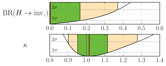
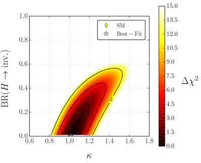
We show the fit results obtained under the assumption of a fully invisible additional Higgs decay mode as one- and two-dimensional profiled distributions in Figs. 1 and 2(a), respectively. The best fit point is found at with a , which corresponds to a -value of . The and ranges are also listed in Tab. 1, along with the corresponding range for the total width scale factor . The two-dimensional distribution in Fig. 2(a) shows a strong positive correlation between and . This reflects the fact that a suppression of the branching ratios to SM particles introduced by an additional invisible decay mode needs to be compensated by an increase of the production rates. The allowed region is however bounded at increasing by the limit from the invisible Higgs search from ATLAS.
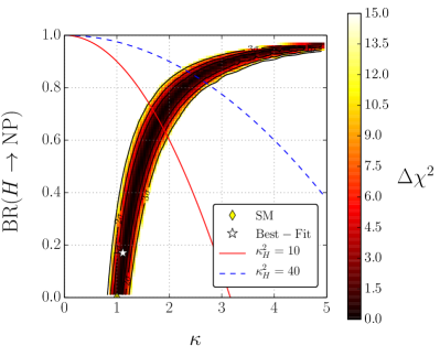
In Fig. 2(b) we illustrate what happens if this constraint is absent, i.e. if no assumptions on the additional Higgs decay mode or model parameters, such as , are imposed. The allowed parameter range then extends towards arbitrarily large values of , and due to the perfect degeneracy mentioned above. In the same figure we indicate present () and potential future () LHC constraints on the total width that could be derived from off-shell Higgs production in Caola:2013yja ; Campbell:2013una . Such upper limits on the total width scale factor, , can be used to infer indirect bounds on and the coupling scale factor .555Note, that this argument applies also for more general, higher-dimensional scale factor models since all scale factors are identical in the degenerate case. Using Eq. (7), the limit can be parametrized by
| (8) |
while SM signal rates are obtained for
| (9) |
For a given upper limit of the total width scale factor, , we can thus infer the indirect bounds
| (10) |
For a current (prospective) upper limit of at the (high-luminosity) LHC, this would translate into and . However, even when taking these constraints into account there remains a quite large parameter space with possibly sizable . Hence, the LHC will not be capable to determine absolute values of the Higgs couplings in a model-independent way. This is reserved for future experiments like the ILC, cf. Sect. 4.2.
Returning to the current fit results displayed in Fig. 2, we can also infer from this fit a lower limit on the total signal strength into known final states (normalized to the SM):
| (11) |
Note, that this limit is irrespective of the final state(s) of the additional Higgs decay mode(s).
3.2 Couplings to gauge bosons and fermions
The next benchmark model contains one universal scale factor for all Higgs couplings to fermions, , and one for the gauge bosons, (). This coupling pattern occurs, for example, in minimal composite Higgs models Agashe:2004rs ; Contino:2006qr ; Giudice:2007fh , where the Higgs couplings to fermions and vector bosons can be suppressed with different factors. The loop-induced coupling scale factors are scaled as expected from the SM structure, Eqs. (5) and (6). Note that scales trivially like in this case, whereas depends on the relative sign of and due to the boson-top quark interference term, giving a negative contribution for equal signs of the fundamental scale factors. Due to this sign dependence we allow for negative values of in the fit, while we restrict . The assumption of universality of the Higgs-gauge boson couplings, , corresponds to the (approximately fulfilled) custodial global symmetry of the SM Higgs sector. We will explore the possibility of non-universal Higgs-gauge boson couplings in the next section.
| Fit parameter | best-fit value | range (1D) | range (1D) |
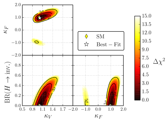
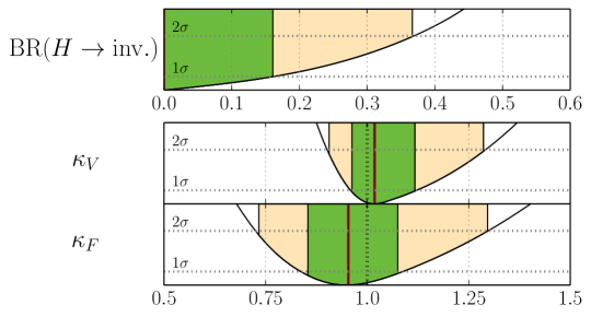
We show the one- and two-dimensional profiled distributions in Figs. 3 and 4, respectively. At the best-fit point we have , corresponding to a -value of . The best-fit values of the fit parameters and the (derived) scale factors for the total width and loop-induced couplings are listed in Tab. 2 including the one-dimensional and ranges. Both the Higgs-fermion couplings and Higgs-gauge boson couplings are very close to their SM values. At most, indicates a very weak tendency to a slight suppression. We can obtain upper limits on the branching ratio to invisible final states, , and the total decay width .
From the two-dimensional profiles, shown in Fig. 4, we see that the sector with negative is disfavored by more than . In the positive sector, and show a strong positive correlation to preserve SM-like relations among the production cross sections and branching ratios. At this stage, due to the assumed scaling universality of all Higgs couplings to fermions and gauge bosons, the fit does not have enough freedom to resolve small potentially present tendencies in the Higgs signal rates, but rather reflects the overall global picture. Hence, we expect the correlation of with the Higgs fermion coupling scale factor(s) to diminish once more freedom is introduced in the Yukawa coupling sector. This will be discussed in Sect. 3.4. Furthermore, Fig. 4 shows that both and are positively correlated with , similarly to the case with an overall coupling scale factor (cf. Fig. 2).
3.3 Probing custodial symmetry
| Fit parameter | best-fit value | range (1D) | range (1D) |
|---|---|---|---|
Experimentally, deviations from the custodial global symmetry are strongly constrained by the oblique (Peskin-Takeuchi) parameter Altarelli:1990zd ; Peskin:1991sw obtained in global electroweak fits Baak:2012kk ; Ciuchini:2013pca . Nevertheless, as an independent and complementary test, it is important to investigate the universality of the Higgs-gauge boson couplings directly using the signal rate measurements.
Here, we restrict the analysis to the simplest benchmark model probing the custodial symmetry, consisting of individual scale factors for the Higgs couplings to and -bosons, and , respectively, and a universal scale factor for the Higgs-fermion couplings, . Again, we also allow for an additional invisible decay mode, . Note that, besides the direct signal rate measurements in the channels and , different constraints apply to the scale factors and : The loop-induced coupling scale factors and are only affected by and , hence plays a subdominant role in the important channel by only affecting the less important production modes and VBF. In contrast, the invisible Higgs search does not constrain at all, but only the product . Since the – boson interference term in the vector boson fusion channel is neglected, we can impose without loss of information. As in Sect. 3.2, we furthermore impose and accommodate the sign dependence in the loop-induced couplings by allowing to take on negative values.
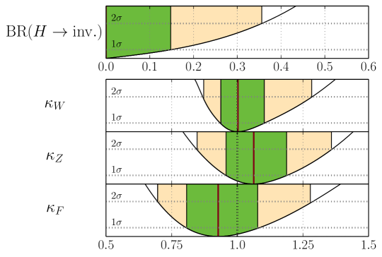
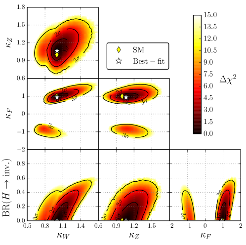
The results of the fit are shown in Figs. 5 and 6 as one- and two-dimensional profiles in the fit parameters. The best-fit values and the (1D) and C.L. intervals of the fit parameters and derived scale factors are listed in Tab. 3. The best fit point features , corresponding to a -value of . Similar as in the previous fit, a very small non-significant suppression of the Higgs-fermion coupling scale factor can be observed. Furthermore, the fit has a small tendency towards slightly enhanced , whereas is very close to the SM value.666A stronger tendency like this was also seen in the official ATLAS result ATLAS:2013sla . Due to the combination with measurements from other experiments, the tendency observed in our fit is much weaker. The Higgs-gauge boson coupling scale factors both agree well with the SM predictions, and also with being equal to each other. Since the fit shows excellent agreement of the data with the assumption of custodial symmetry, we will assume in the following.
As can be seen from the two-dimensional profiles, Fig. 6, the sector with negative is less disfavored than in the previous fit, albeit still by more than . Since the connection between and is dissolved, the signal rates of can be accommodated more easily in the negative sector than before. It can be seen in Fig. 6 that the least constrained region for negative favors values of and , i.e. a much larger discrepancy between and than in the positive sector, where we found the overall best fit.
3.4 Probing the Yukawa structure
| Fit parameter | best-fit value | range (1D) | range (1D) |
|---|---|---|---|
We will now have a closer look at the Higgs-fermion coupling structure. In fact, assuming that all Higgs-fermion couplings can be described by one common scale factor — as we have done until now — is motivated in only a few special BSM realizations. A splitting of up- and down-type Yukawa couplings appears in many BSM models, e.g. Two-Higgs-Doublet Models (2HDM) Lee:1973iz ; Glashow:1976nt ; Deshpande:1977rw ; Donoghue:1978cj ; Haber:1978jt ; Hall:1981bc ; Gunion:2002zf ; Branco:2011iw ; Cheng:1987rs of Type II or in the minimal supersymmetric extension of the SM (MSSM) Haber:1984rc ; Gunion:1984yn ; Gunion:1986nh ; Gunion:1989we . Moreover, realistic 2HDMs with more generic Yukawa couplings featuring additional freedom for the Higgs-charged lepton coupling can be constructed to be consistent with constraints from flavor-changing neutral currents (FCNCs) Cheng:1987rs ; Mahmoudi:2009zx ; Crivellin:2012ye ; Crivellin:2013wna . Also in the MSSM, the degeneracy of bottom-type quarks and leptons can be abrogated by radiative SUSY QCD corrections (so-called corrections) Hempfling:1993kv ; Hall:1993gn ; Carena:1994bv . Therefore, we now relax the assumption of a universal Higgs-fermion coupling scale factor and introduce common scale factors for all up-type quarks, , all down-type quarks, , and all charged leptons, . All Higgs-fermion coupling scale factors are allowed to take positive and negative values. The parameters and remain from before.
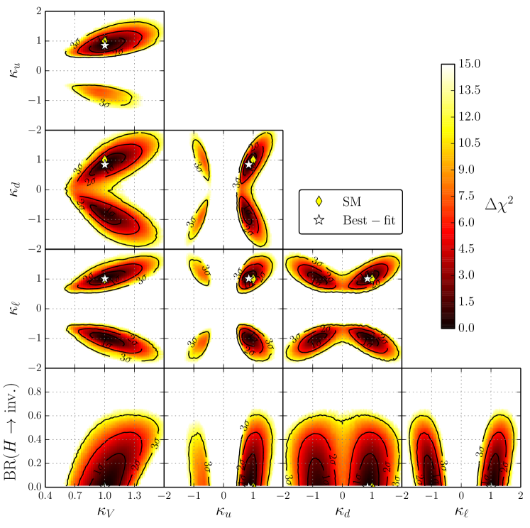
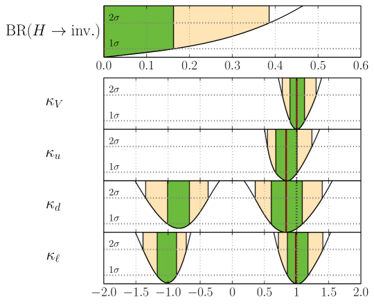
The one-dimensional profiles of the fit parameters are shown in Fig. 7. The parameter values of the best-fit point, which is found in the sector with all scale factors being positive, are given in Tab. 4 along with the (1D) and C.L. intervals. The fit quality is corresponding to a -value of . As can be clearly seen in Fig. 7, negative values of and are still consistent with the measurements within due to their small influence on the loop-induced Higgs couplings to gluons and/or photons. In particular the sign discrimination of is very weak. In contrast, negative values of are disfavored by more than due to the influence on the Higgs-photon effective coupling in the convention . The fit prefers slightly suppressed values of since , Eq. (5), which is sensitively probed by the LHC measurements via the gluon fusion production mode. Due to the recent results from ATLAS ATLAS-CONF-2013-108 and CMS CMS:utj ; Chatrchyan:2014nva ; Chatrchyan:2014vua , is determined to be very close to its SM value with a precision of . We observe a slight but non-signifcant suppression of the Higgs-down type quark coupling, . This scale factor has the worst precision of the fitted parameters, about . The sign degeneracy of is slightly broken via the sensitivity of the Higgs-gluon coupling scale factor to the relative sign of and , cf. Eq. (5).
The correlation of the fitted coupling scale factors can be seen from the shape of the ellipses in the two-dimensional profiles, shown in Fig. 8. The slope of the major axis of the ellipse in the positive sector of the () plane is and thus much shallower than the slopes in the () and () planes, approximately given by and , respectively. Therefore, this parameterization exhibits more freedom to adjust the predicted signal rates to the Tevatron and LHC measurements. Nevertheless, the best-fit point and favored region is in perfect agreement with the SM and thus the additional freedom does not improve the fit quality. Once more precise measurements of the and channels become available, this parametrization can be expected to provide a good test of the SM due to the different correlations among and the Higgs-fermion coupling scale factors.
3.5 Probing new physics in loop-induced couplings
Up to now we have investigated possible modifications of the fundamental tree-level Higgs boson couplings to SM particles and derived the loop-induced couplings to gluons and photons using Eq. (5) and (6), respectively. In this section, we modify these coupling scale factors, and , directly. Such modifications could be introduced by unknown new physics loop contributions, while the tree-level Higgs boson couplings are unaffected. Triggered by the hints in the experimental data for a possible enhancement, new physics sources for modifications of the Higgs-photon coupling have been subject to many recent studies. For instance, charged supersymmetric particles such as light staus Carena:2011aa ; Carena:2012gp ; Basso:2012tr ; Buckley:2012em ; Bechtle:2012jw ; Carena:2013qia and charginos SchmidtHoberg:2012yy ; Hemeda:2013hha could give potentially substantial contributions. In 2HDMs the Higgs-photon coupling can be altered due to contributions from the charged Higgs boson Posch:2010hx ; Drozd:2012vf ; Cordero-Cid:2013sxa , and in the special case of the Inert Doublet Model Arhrib:2012ia ; Goudelis:2013uca ; Krawczyk:2013jta ; Krawczyk:2013pea , modifications of and are indeed the only possible change to the Higgs coupling structure. In addition, many of these models can also feature invisible or undetectable Higgs decays. The effective Higgs-gluon coupling can be modified in supersymmetric models by stop contributions, where one can easily find rate predictions for Higgs production in gluon fusion corresponding to Carena:2013qia ; oai:arXiv.org:hep-ph/9806315 ; oai:arXiv.org:hep-ph/0202167 .
Our fit parametrization represents the case where indirect new physics effects may be visible only in the loop-induced Higgs-gluon and Higgs-photon couplings. Direct modifications to the tree-level couplings, as introduced e.g. if the observed Higgs boson is a mixed state, are neglected. The more general case where all couplings are allowed to vary will be discussed in the next section. Due to the very small branching ratio in the SM, the LHC is not yet sensitive to probe . We therefore set . In addition, here we assume that any additional Higgs decays lead to invisible final states. Undetectable Higgs decays are discussed in Sect. 3.7.
| Fit parameter | best-fit value | range (1D) | range (1D) |
|---|---|---|---|
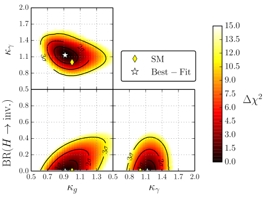
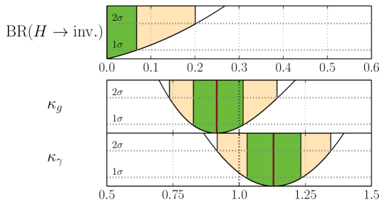
The fit results are shown as one- and two-dimensional profiles in the fit parameters in Fig. 9 and 10, respectively. The (1D) preferred parameter values are also provided in Tab. 5. In this scenario, the best fit indicates a slight suppression of the Higgs-gluon coupling, , with a simultaneous enhancement in the Higgs-photon coupling, . The anti-correlation of these two parameters can be seen in Fig. 10. It is generated by the necessity of having roughly SM-like signal rates. The best fit point, which has , is compatible with the SM expectation at the level, as can be seen in Fig. 10. The estimated -value is . Note that is much stronger constrained to (at ) in this parametrization than in the previous fits. The reason being that the suppression of the SM decay modes with an increasing cannot be fully compensated by an increasing production cross sections since the tree-level Higgs couplings are fixed. The partial compensation that is possible with an increased gluon fusion cross section is reflected in the strong correlation between and , which can be seen in Fig. 10.
3.6 General Higgs couplings
We now allow for genuine new physics contributions to the loop-induced couplings by treating and as free fit parameters in addition to a general parametrization of the Yukawa sector as employed in Sect. 3.4. This gives in total seven free fit parameters, , , , , , and . Note, that this parametrization features a sign degeneracy in all coupling scale factors, since the only derived scale factor, , depends only on the squared coupling scale factors. For practical purposes, we thus restrict ourselves to the sector where all scale factors are positive. Furthermore, it can be illustrative to decompose and into scale factors for the calculable contributions from SM particles, with rescaled couplings, appearing in the loop, as described by Eqs. (5)–(6), and a scale factor for the genuine new physics contributions:
| (12) | ||||
| (13) |
This decomposition assumes that the unknown new physics does not alter the loop contributions from SM particles, Eqs. (5)–(6). Technically, the are used as fit parameters, and the derived are evaluated for each scan point. can thus be extracted for each point, and by this construction, the likelihood distribution in includes the full correlations.
| Fit parameter | best-fit value | range (1D) | range (1D) |
|---|---|---|---|
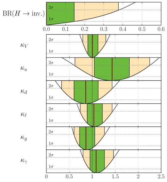
The one-dimensional profiles in the fit parameters are shown in Fig. 11. Their best-fit values and preferred parameter ranges are listed together with those of derived scale factors in Tab. 6. The best-fit point features a fit quality of and thus a -value of . Due to the dissolved dependence between the Yukawa couplings and the effective Higgs-gluon and Higgs-photon couplings, is significantly less accurately determined than in previous more constrained fits. In fact, it is now dominantly influenced by the recent CMS measurements targeting production CMS:2013tfa ; CMS:2013sea ; CMS:2013fda , which give a combined signal strength of CMStthcombination . Hence, the fit prefers slightly enhanced values, , albeit with very large uncertainties. The scale factors and can now be freely adjusted to match the combined rates of Higgs production in gluon fusion and , respectively. Here we observe the same tendencies as in the previous fit, cf. Sect. 3.5. Due to the slight preference for enhanced and suppressed , the fitted new physics contribution to the Higgs-gluon coupling is quite sizable and negative, . In contrast, the Higgs-photon coupling is fairly well described by the rescaled contributions from SM particles alone because the enhanced also enhances slightly. The favored magnitude for the genuine new physics contribution to the Higgs-photon coupling is .
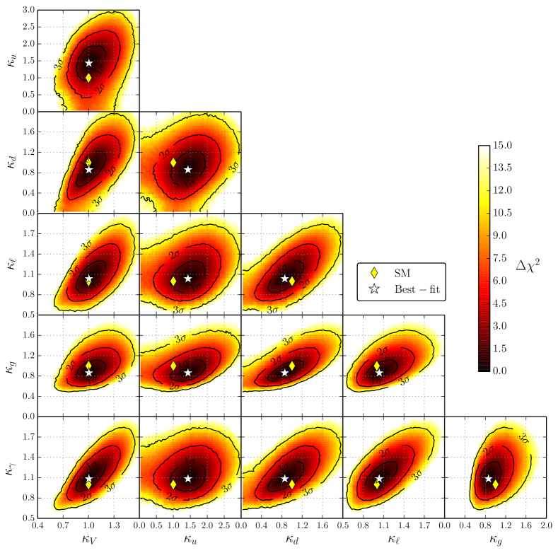
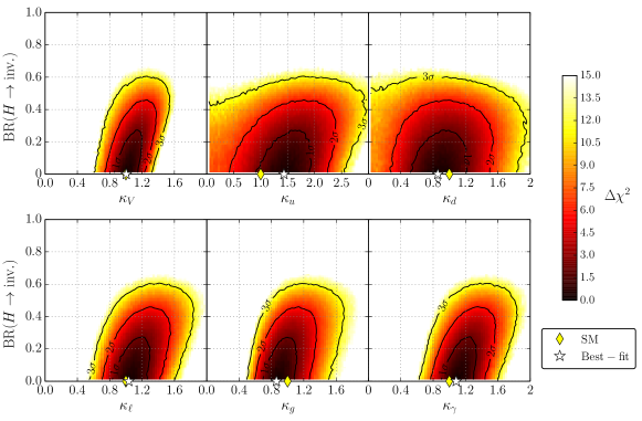
The two-dimensional profiles of the fitted Higgs coupling scale factors are shown Fig. 12 and their correlations with are given in Fig. 13. Similarly as in the fit to the Yukawa structure in Sect. 3.4, all fundamental coupling scale factors are positively correlated. However, the correlations here are much weaker due to the additional freedom introduced for the loop-induced Higgs couplings. In the projection planes for and the Higgs-fermion coupling scale factors, the ellipses are tilted in comparison to the previous fit in Sect. 3.4, now featuring larger slopes of the major axes, which are roughly given by , and for the (), () and () planes, respectively. This represents the fact that , and are less accurately determined since they are now only probed by the poorly measured , and rates, respectively, while is still strongly constrained by both the VBF and production modes and the decay modes and .
The correlations of the fundamental coupling scale factors to the loop-induced couplings scale factors and also turn out to be positive. Here the strongest correlation is observed among and , which govern the dominant production and decay modes, respectively. Since the decay is not yet probed to any reasonable accuracy at the LHC, the fit allows for an enhanced decay rate if at the same time the dominant production cross section is also increased in order to compensate for the reduced branching ratios of the remaining decay modes.777A similar correlation was found in the fit presented in Sect. 3.4 for and , because there was dominantly influencing the derived Higgs-gluon coupling. Nevertheless, the preferred fit region is found for slightly suppressed values of both and . A strong positive correlation is also found between and .
It should be noted that the correlation of the loop-induced couplings scale factors and has changed with respect to the previous fit, Sect. 3.5. They now show a weak positive correlation. This is because the general parametrization features again the degeneracy of increasing scale factors and the additional decay mode, which is only broken by the constraint. This leads to a positive correlation among all which dominates over the small anti-correlations needed to adjust the small tendencies in the observed signal rates. This is also reflected in Fig. 13, where all scale factors show a positive correlation with .
| Fit | precision of the Higgs coupling scale factors [in ] | |||||
|---|---|---|---|---|---|---|
| CMS Moriond 2013 | ||||||
| HiggsSignals (LHC Tev.) | ||||||
Comparing the relative () precision on the individual scale factors obtained here with the results of an official CMS fit analysis888The CMS fit parametrizes the Higgs couplings via the same scale factors as used here, however, the fit does not allow for an additional Higgs decay mode. We furthermore used the CMS fit results to validate our fit procedure, see Appendix A.2. presented at the Moriond 2013 conference CMS:yva , we assert the improvements listed in Tab. 7. Here only rough symmetrical estimates of the sometimes quite asymmetrical uncertainties are given. With a common interpretation of the latest data from ATLAS, CMS and the Tevatron experiments, a significant improvement of the scale factor determination is achieved. Moreover, the strong improvement in the precision of is due to the dedicated CMS tagged analyses CMS:2013tfa ; CMS:2013sea ; CMS:2013fda which had not been included in the CMS fit. With the latest measurement by ATLAS the precision of has also improved significantly. Nevertheless, for all scale factors potential deviations within or even more are still allowed at the level within this benchmark model.
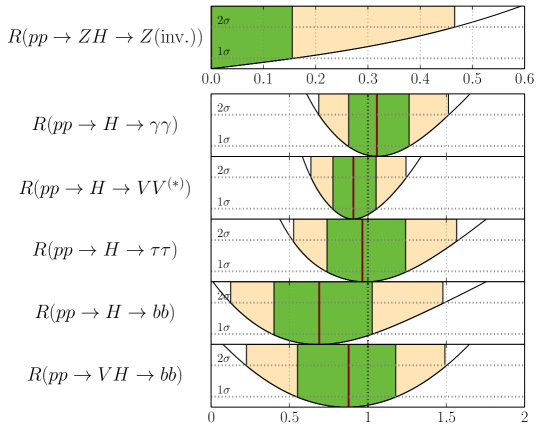
For this most general fit we also show the predicted signal rates for the preferred parameter space in Fig. 14. The rates are idealized LHC signal rates where all included channels contribute with the same efficiency , i.e.,
| (14) |
where is defined in Eq. (1). The production mode denotes inclusive production, i.e. we include all five LHC Higgs production modes at their (rescaled) SM values, whereas the rates denoted by include only production through Higgs-strahlung [and production]. It can be seen from the figure that all rates agree with the SM expectation at A very weak enhancement of the rate is observed, while the remaining channels with fermionic or weak gauge boson final states are slightly suppressed.
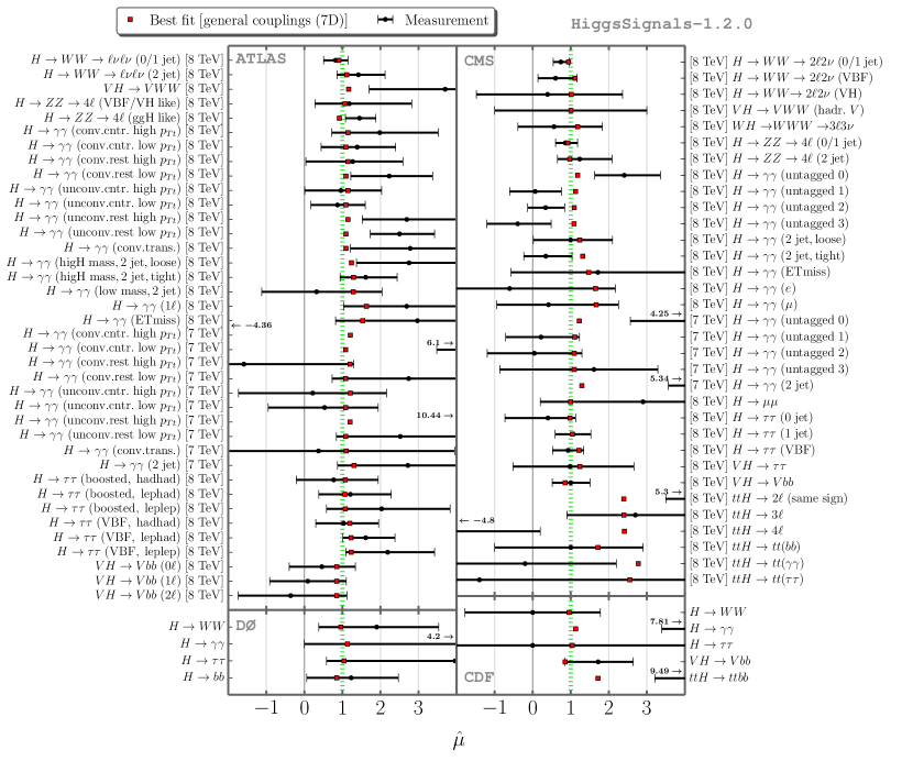
Finally, in Fig. 15 we show the actual signal rates predicted by the best fit point, depicted as red squares, compared to all 80 measurements from the Tevatron and LHC experiments that went into our analysis. The latter are given by the black dots and the error bars indicate the uncertainty. In the left column we show the ATLAS and DØ results, whereas in the right column the CMS and CDF observables are given. The SM, located at , is marked as a green dashed line. It can be seen that most signal rates are predicted to be very close to the SM, note however the relatively large range shown for . An exception can be observed for the channels which comprise a substantial component. Moreover, we find a slight enhancement in channels with a significant contribution from vector boson fusion and/or associated Higgs-weak gauge boson production. Overall, Fig. 15 demonstrates again that despite the large available freedom to adjust the signal rates in this very general parametrization, the preferred region agrees remarkably well with the SM. No significant improvement of the fit quality is gained by allowing the additional freedom. This implies that no significant, genuine tendencies of deviations in the SM Higgs coupling structure can be found.
3.7 Upper limits on additional undetectable Higgs decay modes
We now discuss the case where the additional Higgs decay modes are not detectable with the current Higgs analyses, i.e. their final states do not lead to the missing transverse energy signature, as discussed in the beginning of Sect. 3. As discussed earlier, SM-like Higgs signal rates can be achieved even with a sizable branching fraction to undetectable final states, if at the same time the Higgs boson production rates are enhanced. In the absence of direct measurements of the Higgs total width or absolute cross sections the degeneracy between simultaneously increasing and coupling scale factors can only be ameliorated with further model assumptions. Recall that in general refers to any Higgs decays that are undetectable at present collider experiments, and can in general have both SM or BSM particles in the final state. Requiring that (or and ), an upper limit on can be derived for each investigated benchmark model without assuming that the additional decay modes leads to a missing energy signature.
Remarkably, we find that some of the six benchmark parametrizations discussed in Sect. 3.1–3.6 yield very similar limits on . We therefore categorize them in three Types:
- Type 1:
-
Type 2:
Benchmark models with fixed tree-level couplings but free loop-induced couplings, cf. Sect. 3.5.
- Type 3:
| category | SM | Type 1 | Type 2 | Type 3 |
|---|---|---|---|---|
| Fitted coupling scale factors | - | |||
| () | ||||
| () |
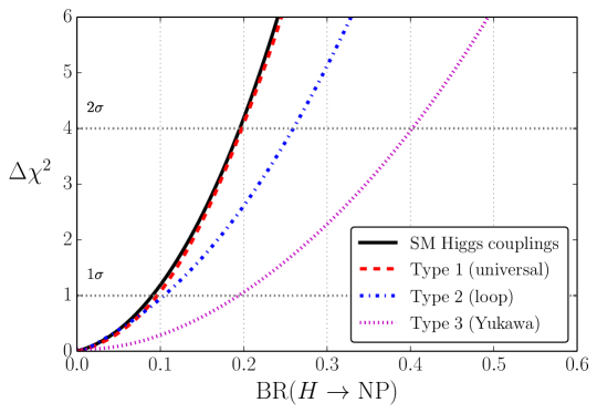
The resulting upper limits on are given in Tab. 8. The corresponding profiled distributions are displayed in Fig. 16. The most stringent limits are obtained for Type 1, where the limit is nearly identical to what is obtained with fixed SM Higgs couplings. The weakest limits are obtained for Type 3. But even in the latter, least restricted case a at the is found.
For some of the benchmark fits considered here a similar study has been performed in Ref. Belanger:2013xza using Moriond 2013 results. The limits presented there are in good agreement with our results.
4 Future precision of Higgs coupling determinations
4.1 Prospective Higgs coupling determination at the LHC
The LHC experiments ATLAS and CMS have provided estimates of the future precision for the Higgs signal rate measurements in most of the relevant channels for integrated luminosities of and at EuropeanStrategyforParticlePhysicsPreparatoryGroup:2013fia . The first numbers (from 2012) have recently been updated ATLAS:2013hta ; ATL-PHYS-PUB-2013-014 ; CMS:2013xfa . In this section we use these updated projections to determine the accuracy of future Higgs coupling determination at the LHC. Similar studies based on the updated projections were recently performed in Refs. Dawson:2013bba ; Peskin:2013xra , using a slightly different methodology and parametrization of the Higgs couplings. For earlier studies see also Refs. Zeppenfeld:2000td ; Duhrssen:2004cv ; Duhrssen:2004uu ; Lafaye:2009vr ; Klute:2012pu ; Klute:2013cx .
Concerning the projected sensitivities for rate measurements from ATLAS, a detailed compilation has been provided in Refs. ATLAS:2013hta ; ATL-PHYS-PUB-2013-014 which in most cases contains information on the signal composition, and the projections are given with and without theoretical uncertainties. ATLAS has also provided projections for sub-channels including tags for the different production modes. Unfortunately, a projection for the important channel is not yet available. This channel plays an important role in any global fit, since the partial decay width for dominates the total width in the SM. Moreover, the ATLAS projection is based on an older analysis, and one could expect a potential improvement from an updated study.
CMS has provided estimates for the capabilities to measure the Higgs signal rates only for inclusive channels CMS:2013xfa . Unfortunately, detailed information about the signal composition is missing. We are therefore forced here to assume typical values for the signal efficiencies guided by present LHC measurements. Moreover, the treatment of theoretical uncertainties in the CMS projections is not very transparent.999See also Ref. Peskin:2013xra for a discussion of this issue. CMS discusses two scenarios: Scenario 1 uses current systematic and theoretical uncertainties.101010Note that improvements of systematical uncertainties that can be reduced with increasing statistics in the data control regions are however taken into account. Furthermore, even the assumption that the same systematical uncertainties as at present can be reached for the harsher experimental conditions in future is based on a projection involving a certain degree of improvement. In Scenario 2 the theoretical uncertainties are reduced by , whereas the experimental systematic uncertainties are decreased with the square root of the integrated luminosity. No projections without theoretical uncertainties are provided by CMS. However, the Scenario 2 projections appear quite aggressive since they are of the same order as — or even more precise than — the purely experimental projections from ATLAS. Furthermore, our estimates of theoretical uncertainties, rescaled under the assumptions of Scenario 2, yield in some cases, e.g. in the and channels with , values that are larger than the CMS estimates of the total (i.e., theoretical and experimental) uncertainties of the measurements, at least when assuming that the main production mechanism for the signal is gluon fusion. Following a conservative approach, we therefore use the projected CMS rate measurements given for Scenario 2, but interpret the uncertainties as being purely experimental.111111Another way to circumvent this problem is discussed in Ref. Peskin:2013xra , where an alternative set of projected CMS measurements is proposed. However, it should be noted that the dominant effect leading to differences between our results and the official CMS estimates of prospective Higgs coupling determination is the absence of publicly available CMS projections of the category measurements. Using only the inclusive measurements generally leads to lower precision estimates in higher-dimensional scale factor fits.
[b] Future scenario PDF , , THU constraint LHC300 (S1) all conservative, Eq. (16) LHC300 (S2, csv.) all conservative, Eq. (16) LHC300 (S2, opt.) all optimistic, Eq. (18) HL–LHC (S1) all conservative, Eq. (17) HL–LHC (S2, csv.) all conservative, Eq. (17) HL–LHC (S2, opt.) all optimistic, Eq. (19) ILC250 - all (cf. Tab. 16) ILC500 - all (cf. Tab. 16) ILC1000 - all (cf. Tab. 16) ILC1000 (LumiUp) - all (cf. Tab. 16) HL–LHC ILC250 () all HL–LHC ILC250 all HL–LHC ILC500 all HL–LHC ILC1000 all HL–LHC ILC1000 (LumiUp) all
-
Affects the theoretical uncertainties (THU) of all partial widths except for the decay modes and (kept unchanged) as well as the uncertainties from missing higher-order QCD corrections, often estimated via a scale variation, and missing higher-order EW corrections for all LHC production modes.
-
In this scenario only the direct ILC measurement of with at is added to the HL–LHC projections to constrain the total width.
-
*
For the HL–LHC ILC combinations we do not use the assumption .
The ATLAS and CMS estimates of the experimental precision used in our analysis are listed in Tab. 15 in Appendix A.3, which also gives the assumed signal composition for each channel. For both experiments we assume that the experimental precision includes a systematic uncertainty on the integrated luminosity, which is treated as fully correlated among each experiment.
On top of these experimental precisions we add theoretical rate uncertainties within HiggsSignals. We discuss two future scenarios for the LHC-only projections: In the first scenario (S1) we take the current theoretical uncertainties as already used in the previous fits in Sect. 3. This scenario thus represents the rather pessimistic — or conservative — case that no improvement in the theoretical uncertainties can be achieved. With increasing integrated luminosity, however, the uncertainty from the parton density functions (PDF) can be expected to decrease Campbell:2013qaa . Future progress can also be expected in calculations of higher-order corrections to the Higgs production cross sections and decay widths, which may further decrease the theoretical uncertainties, in particular the QCD scale dependence and remaining uncertainties from unknown electroweak (EW) corrections. Hence, in the second scenario (S2) we assume that uncertainties from the PDFs, as well as most121212This includes uncertainties from missing higher-order QCD corrections, often estimated by scale variation, and unknown EW corrections for the LHC Higgs production modes, as well as the uncertainties of all partial decay widths except the decays to and bosons where higher-order EW corrections are already known with high accuracy. theoretical uncertainties, are halved. In both scenarios, the parametric uncertainties from the strong coupling constant, , and the heavy quark masses, , and , are unchanged. The different future scenarios considered in our analysis together with the respective assumptions on the future uncertainties and constraints are summarized in Tab. 9. The entry “100%” in Tab. 9 corresponds to the present value of the considered quantity, and accordingly, “50%” denotes an improvement by a factor of two. More details and estimates of the cross section and branching ratio uncertainties for these scenarios are given in Appendix C.
ATLAS and CMS also provide projections for the upper limit on the rate of an invisibly decaying Higgs boson in the Higgs-strahlung process, . Assuming, like we have done in Sect. 3.1–3.6, that additional Higgs decay modes give rise to purely invisible final states131313We state explicitly in Tab. 9 which constraint on the additional decay modes is applied, if purely invisible final states are assumed., these constraints are incorporated in our fit as ideal likelihoods of the form
| (15) |
The quantity corresponds to the product , i.e the cross section of normalized to the SM cross section for . Both ATLAS and CMS consider two scenarios for the projected limits ATL-PHYS-PUB-2013-014 ; CMS:2013xfa : The conservative (csv.) scenario,
| (16) | ||||
| (17) |
and the optimistic (opt.) scenario,
| (18) | ||||
| (19) |
We combine the projected ATLAS and CMS limits by adding their respective contributions. For the scenario S1 we only employ the conservative constraints, Eqs. (16) and (17), whereas for the scenario S2 with reduced uncertainties we compare fits using either the conservative or the optimistic constraint. These cases are denoted by (S2, csv.) and (S2, opt.), respectively.
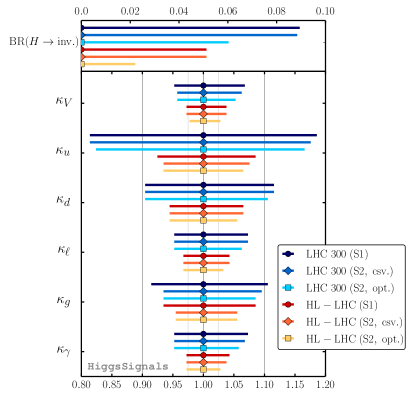
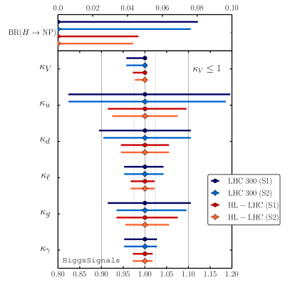
For the LHC projections we employ the same seven-dimensional scale factor parametrization as discussed in Sect. 3.6. The resulting precision estimates obtained under the assumption that the additional decay mode are displayed in Fig. 17(a) and listed in Tab. 10. The plot includes all six LHC-only scenarios as listed in Tab. 9.
In general the obtained limit on is weaker than the limit obtained from a Gaussian combination of the limits in Eqs. (16)–(19), because the fit has the freedom to adjust to values . Improvements in the theoretical uncertainties will mostly affect the effective Higgs-gluon coupling. At an integrated luminosity of we obtain a precision estimate for the scale factor of the effective Higgs-gluon coupling of in the more conservative scenario S1,141414Here and in the following the Higgs coupling precision at is denoted by . The values quoted in the text usually correspond to symmetric averages. For the exact asymmetric values see the corresponding tables, e.g. here Tab. 10. which is improved to in the most optimistic scenario S2. At the high luminosity LHC with the corresponding projections are for the scenario S1 and for the scenario S2, irrespective of the assumed precision of the constraint. The assumed improvements of the theoretical uncertainties hence lead to a significant increase of the precision at the HL–LHC, while the precision at is still mostly limited by statistics.
The impact of more optimistic limits on the invisible Higgs decays, Eqs. (18)–(19), can directly be seen in the projected upper limit on in Fig. 17(a). Since this improved constraint also applies to the Higgs– boson coupling the precision of the Higgs–vector-boson coupling scale factor, , also improves from [] to [] at [], assuming the improved theoretical uncertainties of Scenario S2. The impact on the remaining scale factors is rather insignificant and results mostly from their positive correlation with and . Hence, these are slightly more constrained from above if a more optimistic limit on the invisible Higgs decays can be achieved.
| Higgs coupling scale factor precision [in ] | ||||||
| LHC 300 | HL–LHC | |||||
| \rowfont Scenario | S1 | S2, csv. | S2, opt. | S1 | S2, csv. | S2, opt. |
| \rowfont | ||||||
| Higgs coupling scale factor precision [in ] | ||||
| LHC 300 | HL–LHC | |||
| \rowfont Scenario | S1 | S2 | S1 | S2 |
| \rowfont | ||||
Taking into account the possibility that an additional Higgs decay mode may result in an undetectable final state, we show the fit results obtained under the assumption in Fig. 17(b) and Tab. 11. Overall, the achievable precision in the Higgs coupling scale factors with this assumption on the Higgs coupling to gauge bosons is very similar to what was obtained with the assumption of allowing only additional Higgs decays into invisible final states, cf. Fig. 17(a). A notable difference is, however, that in particular the scale factors and are more strongly constrained from above due to their positive correlation with , which is forced to be by assumption in this case. The obtained limit projection on can be regarded as an independent limit projection inferred from the model assumption on and the chosen parametrization, see also the discussion in Sect. 3.7. Remarkably, the limit projections obtained here are stronger than the allowed range for in the previous fits in Fig. 17(a) where the constraints from searches for an invisibly decaying Higgs boson have been applied.
Overall, we find estimates of Higgs coupling scale factor precisions within at and at obtained under the assumption . These estimates improve slightly if one assumes instead. Comparisons with results in the literature based on the same projections of the future capabilities provided by ATLAS and CMS, our results agree quite well with those presented in Ref. Dawson:2013bba . A comparison of our results with Ref. Peskin:2013xra would need to take into account the different approaches of implementing the CMS projections. In view of this fact, we also find reasonable agreement with the results presented in Ref. Peskin:2013xra .
It should be noted that this seven-parameter fit within the “interim framework” of Higgs-coupling scale factors still contains important simplifying assumptions and restrictions, which one would want to avoid as much as possible in a realistic analysis at the time when or of integrated luminosity will have been collected, see the discussion in Refs. LHCHiggsCrossSectionWorkingGroup:2012nn ; Heinemeyer:2013tqa .
4.2 Prospective Higgs coupling determination at the ILC
Looking beyond the LHC, an linear collider (LC) with a center-of-mass energy that can be raised at least up to is widely regarded to be ideally suited for studying the properties of the discovered new particle with high precision. The Technical Design Report for the International Linear Collider, ILC, has recently been submitted Baer:2013cma , and there are encouraging signs that a timely realisation of this project may become possible due to the strong interest of the Japanese scientific community and the Japanese government to host the ILC.
The ILC offers a clean experimental environment enabling precision measurements of the Higgs boson mass, width, its quantum numbers and -properties as well as the signal rates of a variety of production and decay channels, including a high-precision measurement of the decay rate into invisible final states. The highest statistics can be accumulated at the highest energy, , from the -channel process where a Higgs boson is produced in fusion (). At an absolute measurement of the production cross section can be performed from the Higgs-strahlung process () near threshold using the recoil of the Higgs boson against the boson, decaying via or , without having to consider the actual pattern of the Higgs decay. The absolute measurement of the production cross section can be exploited to obtain absolute measurements of the decay branching ratios and of the total width of the decaying particle. Consequently, no additional model assumptions are necessary to constrain the total width and thus the Higgs boson couplings. For an integrated luminosity of will result in Higgs bosons. The ILC will provide high-precision measurements of channels that are known to be difficult (such as ) or may even be impossible (such as ) at the LHC. At the weak boson fusion process already dominates over the Higgs-strahlung process for a SM-like Higgs boson, and the two production channels together provide data with very high statistics. Starting from this energy, the top Yukawa coupling and, for sufficiently high luminosity, the trilinear self-coupling will become accessible.
In this section we study the capabilities of Higgs coupling determinations at the ILC. Similar studies have been performed in Ref. Klute:2013cx ; Han:2013kya ; Dawson:2013bba ; Peskin:2013xra . We discuss fit results using prospective ILC measurements both alone and in combination with measurements from the HL–LHC. Since the two major Higgs production modes, Higgs-strahlung and fusion, are governed by the Higgs-- and Higgs-- couplings, respectively, from now on we abandon the assumption of custodial symmetry. In comparison to the LHC, the sensitivity to probe custodial symmetry is greatly enhanced at the ILC, since clean measurements of the two main production modes can be performed individually at high precision. Instead of the previous parametrization, we fit individual scale factors for the Higgs-- and Higgs-- couplings from now on. Thus, we employ an eight-dimensional fit in the parameters , , , , , , and .
The projected ILC measurements have been presented in Ref. Baer:2013cma and recently updated in a Snowmass White paper Asner:2013psa . These updated numbers, which we use in our fits, are summarized in Tab. 16 in Appendix A.3. In particular, we include the measurements of the total cross section, cf. Tab. 16, which constrain the total width and enable a model-independent determination of the Higgs couplings. An assumed luminosity uncertainty of and theoretical uncertainties of the , and cross section predictions of , and , respectively, are treated as fully correlated in our fit. We assume the same improvements of the theoretical uncertainties for the Higgs decay modes as in Scenario S2 of the LHC projections. In addition, we assume that the parametric uncertainties from dependences on and the heavy quark masses , and can also be reduced by with prospective ILC measurements and lattice calculations Campbell:2013qaa . A further reduction of the top quark mass uncertainty — anticipated to improve by a factor of with respect to the current precision Baer:2013cma — has negligible impact on the partial width uncertainties is and therefore not further considered here. A summary of all future scenarios that we consider in our analysis is given in Tab. 9. Estimates of the theoretical uncertainties on the Higgs branching ratios that we apply for the ILC scenarios are provided in Appendix C.
In our analysis of the ILC projections we consider three stages of center-of-mass energies, namely (stage 1), (stage 2) and (stage 3). For the integrated luminosities at those energy stages we investigate both a baseline program with integrated luminosities of at stage 1, at stage 2 and at stage 3, as well as a scenario corresponding to a luminosity upgrade (LumiUp). For the latter the integrated luminosities of at stage 1, at stage 2 and at stage 3 are assumed, see Ref. Asner:2013psa .
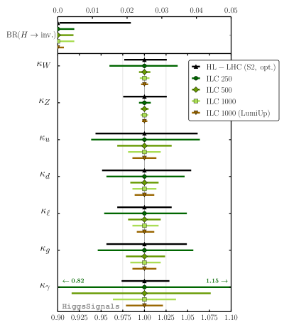
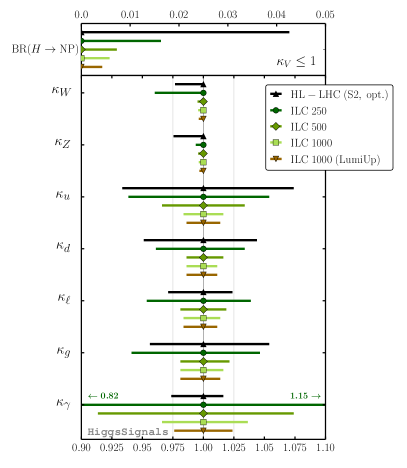
In Fig. 18 we show the estimated accuracies of the Higgs coupling scale factors at the ILC obtained under model-dependent assumptions, in analogy to the analyses performed above for the projections of future accuracies at the LHC: In Fig. 18(a) we assume that any additional Higgs decay results in invisible final states; accordingly we also take into account the projected ILC upper limit on , cf. Tab. 16 (or Tab. 9). In Fig. 18(b) we apply the theoretical constraint . For comparison we also show the fit results for the optimistic HL–LHC scenario (S2, opt) obtained under these assumptions.
Overall, the scale factor precisions achieved under those two assumptions are very similar to each other. Comparing the results of the first ILC stage, where just a ‘baseline’ value for the integrated luminosity of is assumed (ILC250), with the ultimate precision that can be reached at the LHC, we see already at this stage a substantial improvement in the precision of the scale factor (from to ). This is already a crucial improvement since this coupling is of central importance in the experimental test of the electroweak symmetry breaking mechanism. Furthermore, the ILC provides at this stage important measurements that are complementary to the HL–LHC measurements. For instance, the independent determination of the Higgs coupling to gluons via the decay is advantageous in order to eliminate the dependence of this quantity on the remaining PDF uncertainties of the LHC gluon fusion process. In addition, the measurement of the rate with 1.2% accuracy, see Tab. 16, together with the absolute cross section measurement of the production process with a precision of , give important constraints on the decay mode, which dominantly contributes to the total width of a SM-like Higgs boson. However, the corresponding scale factors and are still strongly correlated. Another independent measurement of the mode with similar precision — as it is provided e.g. at the ILC stage 2 with in fusion (see below) — is required to abrogate this correlation, thus allowing for a precise determination of .
The most striking improvement that the ILC already provides at the first stage with , however, is the model-independent measurement of the production process and correspondingly model-independent determinations of Higgs branching ratios. Combining this input from the ILC with the measurements performed at the HL–LHC leads to a significant improvement of the latter, as will be discussed below (see Fig. 19).
While can be probed already quite accurately at the early ILC stage at due to the dominant Higgs-strahlung process, the determination is less precise, . This picture changes at the later stages of the ILC with higher center-of-mass energies, denoted as ILC500 and ILC1000, where the ‘baseline’ integrated luminosities of and , respectively, have been assumed. At ILC500 and ILC1000 the fusion becomes the dominant production mode. Here, all scale factors in this parametrization except can be determined to a precision of better than using only ILC measurements. With the ultimate ILC integrated luminosity, denoted as ILC1000 (LumiUp), even the coupling can be probed with an accuracy of , and the remaining couplings are determined at the level, again using ILC measurements only. In the case where is imposed instead of assuming non-standard Higgs decays to result in invisible final states, the sensitivity for setting an upper limit on inferred from the fit improves significantly at the ILC from to at the .
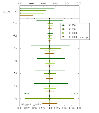
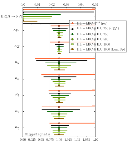
As stated earlier, the assumptions made in the previous fits are actually unnecessary at the ILC once the total cross section measurement of the process is taken into account. Therefore, model-independent estimates of the Higgs coupling accuracies can be obtained, which are shown in Fig. 19(a) and (b) for the ILC only and HL–LHC ILC combined measurements, respectively. The values are also listed in Tab. 12. The estimated accuracies obtained for the ILC-only measurements in this model-independent approach are only slightly weaker than the ones obtained above under additional model assumptions, cf. Fig. 18. At the early ILC stage (ILC250) the sensitivity for setting a model-independent upper limit on of is obtained from the fit. This sensitivity improves to at the later baseline ILC stages. The more precise measurement of the cross section at with the ILC luminosity upgrade improves the sensitivity further, such that at can be reached at the ultimate ILC stage at .
For the combination of HL–LHC and ILC measurements for a model-independent Higgs coupling determination, as shown in Fig. 19(b), it is illustrative to consider first the results obtained using the HL–LHC only or with a minimal amount of ILC input, i.e. by only adding the total cross section measurement of the process. In the first case, as already demonstrated in Sect. 3.1, the unconstrained fit (HL–LHC ( free) in Fig. 19(b)) features a degeneracy of increasing and increasing scale factors , until the LHC is finally capable to observe broad width effects via off-shell Higgs production. As a result, there is virtually no sensitivity in determining an upper limit for very large values of the scale factors.151515The fact that the error bars for the scenario HL–LHC ( free) extend to values far outside of the right-hand side of Fig. 19(b) is indicated by little arrows in the plot.
| Higgs coupling scale factor precision [in ] | |||||||||
| ILC only | HL–LHC ILC | ||||||||
| \rowfont Scenario | 250 | 500 | 1000 | 1000 (LumiUp) | 250 () | 250 | 500 | 1000 | 1000 (LumiUp) |
| \rowfont | |||||||||
By adding only the total cross section measurement from the baseline ILC250 run to the HL–LHC observables the degeneracy is broken. This leads to a very significant improvement in the determination of all Higgs coupling scale factors. Besides this effect one can see that the combination with this single input value from the ILC leads to further significant improvements affecting also the lower limits on the scale factors. In particular, the precision on the lower limit of improves from to . Moreover, the upper limit on inferred from this fit without any additional assumptions is . This is roughly comparable to what has been obtained under the additional model assumptions in the LHC-only fit, cf. Fig. 18(b). With the inclusion of the remaining ILC measurements from the baseline run all scale factors except and can be measured at the level. and can be determined with a precision of and , respectively. The only scale factor that is dominantly constrained by the LHC data is that for the Higgs-photon coupling, , which remains the case even at the later ILC stages at and . With the ultimate ILC luminosity, including the upgrade, and combining all available measurements from the HL–LHC and ILC, all Higgs coupling scale factors are probed to at least a precision of . The Higgs-weak gauge boson couplings can even be probed at the per-mille level. At this level the estimated accuracies are dominated by the assumed (reduced) theory uncertainties. We find that our estimates for the later ILC stages have a slight tendency to be more conservative than those of e.g. Refs. Dawson:2013bba ; Peskin:2013xra , since we include larger theoretical uncertainties for the ILC production cross sections and their correlations.
5 Conclusions
In this paper we have investigated in detail whether the coupling properties of the discovered new particle show any significant deviations from the predictions for a SM Higgs boson at the present level of accuracy. We have further analyzed the room for potential coupling deviations, which remain consistent with the current measurements, and the associated parameter correlations. The study has been carried out within a consistent statistical framework using all available Higgs signal rate measurements from the LHC and Tevatron experiments by employing profile likelihood fits of Higgs coupling scale factors by means of the public program HiggsSignals. The fits have been done both for highly constrained and very generic scale factor parametrizations of the Higgs couplings. All benchmark fits allow for additional Higgs decays to non-standard final states and various assumptions are discussed for constraining the total Higgs decay width at the LHC. In contrast to other investigations in the literature, we have paid particular attention to the treatment of the general case where no constraint on the total Higgs width — or on the branching fraction of Higgs decays to potentially undetectable final states of new physics — is assumed.
We have employed the “interim framework” of Higgs coupling scale factors as a means to parametrize the relations between the physical collider observables (cross sections, branching ratios) and the possible deviations in the couplings of the new state from the predictions for a SM Higgs boson. While the scale factors probe different possible aspects of deviations from the SM predictions, their inherent simplifications and restrictions make it non-trivial to directly map the results obtained in terms of Higgs coupling scale factors onto realistic models of physics beyond the SM. The latter typically predict certain correlations that differ from those assumed for the Higgs coupling scale factors. The investigation of particular models is therefore complementary to the analysis of Higgs coupling scale factors. The tool HiggsSignals, which has been used in the present analysis, has been specifically designed for this purpose, and the statistical methods employed here can be directly taken over for fits of realistic new physics models.
The program HiggsSignals is a well-validated and accurate tool for the evaluation based on the signal rate predictions and the currently 80 included measurements from ATLAS, CMS, CDF and DØ. It takes into account the correlations of luminosity, cross section and branching ratio uncertainties among the signal rate measurements, as well as intrinsic correlations among the cross section and branching ratio uncertainties induced by common parametric uncertainties. For this study, we have further included the correlations of the remaining major experimental systematics for the ATLAS and CMS measurements. We validated the implementation against an official six-dimensional scale factor fit performed by CMS, yielding very good agreement. All these new developments, as documented here, will be provided with HiggsSignals version 1.2.0.
For all considered scale factor benchmark models we find very good agreement between the LHC and Tevatron measurements and the signal rates predicted for the SM. For the SM itself, i.e. all scale factors are set to unity, we find a naive -value of , showing good agreement between data and theory. Thus, it is not surprising that the benchmark models achieve similar -values, which we have found to be typically slightly lower than the SM -value due to the smaller number of degrees of freedom at similar minimal . The lowest -value of is obtained for the fit probing the Yukawa structure in Sect. 3.4, while the best -value, excluding the SM -value, is found with for the benchmark fit probing the loop-induced Higgs couplings to gluons and photons, cf. Sect. 3.5.
We find no indicative hint for deviations from the SM in any of the fits. Indeed, all central values of the fitted Higgs coupling scale factors are compatible with their SM values. The fitted values of an additional Higgs branching fraction, , are also compatible with zero. Uncertainties on the fitted scale factors range from around in the most constrained case, i.e. a fit of only one universal scaling parameter, up to for the top Yukawa scale factor, , in the seven-dimensional fit discussed in Sect. 3.6. Comparing these results with the latest official scale factor determination performed by CMS for the Moriond 2013 conference, we find significant improvements in all scale factor precisions. This illustrates the power of a common interpretation of ATLAS and CMS (and Tevatron) measurements, as well as the importance of the recent measurements in the ATLAS and CMS -tagged searches.
The corresponding weakest observed limit from the fits on the invisible Higgs decay is at the , also taking into account direct searches for at the LHC. We furthermore find for the total signal strength to known SM final states a lower limit of at the CL, employing the benchmark fit with one universal Higgs coupling scale factor . This limit is independent of any further assumption, such as e.g. . Moreover, under the assumption that holds, we find from the most general fit to the present data, which has seven free parameters, the limit at the C.L., where the final state(s) of such Higgs decay(s) may be undetectable to current LHC experiments.
Beyond the current measurements from the LHC and the Tevatron, we have explored the capabilities of future Higgs coupling determinations using projections of the signal rate measurements for the LHC with (LHC 300) and (HL–LHC) at , as well as for various scenarios of an International Linear Collider (ILC). At the LHC 300 we find estimated precisions for the determination of the Higgs coupling scale factors within under the assumption . Possible improvements of theoretical uncertainties on the cross sections and branching ratios turn out to have only a marginal effect on those estimated precisions. This changes at the HL–LHC, where the achievable precision of the Higgs-gluon coupling scale factor is significantly limited by the theoretical uncertainty. The precision estimates of the remaining scale factors, however, are hardly affected by varying assumptions on the theoretical uncertainties. Overall, assuming , we find scale factor precisions of at the HL–LHC. If we make the model assumption instead of the assumption that additional non-standard Higgs decays result only in invisible final states, then most of the estimated scale factor precisions marginally improve.
Concerning the prospects at the ILC, we have compared the ILC capabilities of determining Higgs couplings with those of the HL–LHC first for a model-dependent approach, i.e. using the same assumptions as for the HL–LHC analyses, namely assuming either or as a means to constrain the total width. We find that already ILC measurements at for ‘baseline’ assumptions on the integrated luminosity provide significant improvements compared to the most optimistic scenario for the HL–LHC along with complementary measurements that are of similar or slightly worse accuracy compared with the projections for the HL–LHC. Starting from a center-of-mass energy of for the corresponding ‘baseline’ luminosity assumption the ILC in fact has the potential to considerably improve upon all measurements of the HL–LHC apart from the coupling of the Higgs to photons. At , the fusion channel can be measured significantly better than at , which leads to a significantly higher statistics for all considered quantities and in particular to a further improvement in the determination of the total width. The further improvements from ILC running at and from exploiting the ultimate ILC luminosity (LumiUp) turn out to be rather moderate for the considered case of a model-dependent 8-parameter fit, which is related to our fairly conservative estimates of the future theoretical uncertainties.
The impact of the ILC on improving the determination of the Higgs couplings becomes apparent most strikingly for the model-independent analyses. Without employing additional theoretical assumptions the scale factors at the LHC are essentially unconstrained from above. However, taking into account a single measurement of the ILC — the decay-mode independent recoil analysis of the total Higgs production rate at — in conjunction with the HL–LHC measurements already allows to perform a significantly less model-dependent and more precise fit than with the HL–LHC alone. In particular, with this ILC measurement the assumptions on the additional Higgs decay modes and on can be dropped.
From prospective measurements at the ILC up to with the ‘baseline’ assumptions for the integrated luminosity together with those from the HL–LHC, we find precision estimates for all fitted Higgs coupling scale factors of better than . For some scale factors a precision better than is achieved. These estimates are obtained with the least amount of model assumptions and 8 free fit parameters. With the ultimate ILC luminosity (LumiUp) this precision would further increase significantly, reaching a level of better than for all scale factors.
The Higgs coupling scale factor benchmark scenarios considered in this study typically have more freedom to adjust the predicted signal rates to the measurements than realistic models. Realistic model generally feature specific correlations among the predicted rates which depend non-trivially on the model parameters. Moreover, limits from the electroweak precision data and other sectors, such as dark matter, collider searches, etc., may further restrict the allowed parameter space and thus the room for Higgs coupling deviations. The fact that the exploration of the Higgs couplings with those rather general parametrizations does not improve the fit quality with respect to the SM is a clear indication of the good agreement of the data with the SM predictions. On the basis of this analysis one would not expect a significant improvement in the description of the data from a realistic model of physics beyond the SM. Thus, the full set of the present public measurements from ATLAS, CMS, CDF and DØ in the Higgs sector does not show any indications for physics beyond the SM.
Despite the lack of a concrete hint for any deviation from the SM in the current measurements, there still is ample room for future discoveries of deviations from the SM predictions for the Higgs couplings. In fact, the current uncertainties are still rather large and thus still allow for sizable deviations from the SM at the level of at the level, even when making additional theory assumptions, namely or . Comparing those accuracies with the typical deviations expected in realistic models of physics beyond the SM, a large improvement in the experimental precision will be needed in order to sensitively probe the parameter space of the most popular extensions of the SM. The measurements at an ILC-like machine, in conjunction with the HL–LHC, will be crucial in this context for model-independent determinations of absolute Higgs couplings with precisions at the percent level or better, offering great prospects for identifying the underlying mechanism of electroweak symmetry breaking.
Acknowledgements.
We thank Andre David, Ansgar Denner, Klaus Desch, Manuel Drees, Michael Duehrssen, Howie Haber, Alex Read, Björn Sarrazin, Daniel Schmeier and Tom Zirke for helpful discussions. Part of the numerical calculations were performed using the computing infrastructure Campos:2012vb at the “Instituto de Física de Cantabria”. This work was partially supported by the Helmholtz Alliance “Physics at the Terascale”, the Collaborative Research Center SFB676 of the DFG, “Particles, Strings and the early Universe”, and by the European Commission through the “HiggsTools” Initial Training Network PITN-GA-2012-316704. The work of T.S. was supported by the BMBF Grant No. 00160200 and the Bonn-Cologne Graduate School (BCGS). S.H. was supported by CICYT (Grant No. FPA 2010–22163-C02-01) and by the Spanish MICINN’s Consolider-Ingenio 2010 Program under Grant MultiDark No. CSD2009-00064. O.S. is supported by the Swedish Research Council (VR) through the Oskar Klein Centre. Since one of the authors (P.B.) is also an ATLAS member, we would like to clarify that the work presented here is the responsibility of the individual authors and does not represent an ATLAS result. This phenomenological analysis is purely based on public information.Appendix A Experimental data
A.1 Implementation of current signal strength measurements
Tables 13 and 14 list the signal strength measurements from ATLAS, CDF, CMS and DØ as implemented in HiggsSignals-1.2.0; there are 80 observables in total. The tables also provide numbers for the assumed signal composition of a SM Higgs boson for all measurements. Most of these results are used directly in the fits in Sect. 3, except for a few cases where a more careful treatment is required as described in detail below.
[b] Analysis energy SM signal composition [in %] ggH VBF WH ZH ATL (0/1jet) ATLAS:2013wla ; Aad:2013wqa ATL (VBF) ATLAS:2013wla ; Aad:2013wqa ATL (VBF/VH-like) ATLAS:2013nma ; Aad:2013wqa ATL (ggH-like) ATLAS:2013nma ; Aad:2013wqa ATL (unconv.-central-low ) ATLAS:2012goa ATL (unconv.-central-high ) ATLAS:2012goa ATL (unconv.-rest-low ) ATLAS:2012goa ATL (unconv.-rest-high ) ATLAS:2012goa ATL (conv.-central-low ) ATLAS:2012goa ATL (conv.-central-high ) ATLAS:2012goa ATL (conv.-rest-low ) ATLAS:2012goa ATL (conv.-rest-high ) ATLAS:2012goa ATL (conv.-trans.) ATLAS:2012goa ATL (2 jet) ATLAS:2012goa ATL (unconv.-central-low ) ATLAS:2013oma ATL (unconv.-central-high ) ATLAS:2013oma ATL (unconv.-rest-low ) ATLAS:2013oma ATL (unconv.-rest-high ) ATLAS:2013oma ATL (conv.-central-low ) ATLAS:2013oma ATL (conv.-central-high ) ATLAS:2013oma ATL (conv.-rest-low ) ATLAS:2013oma ATL (conv.-rest-high ) ATLAS:2013oma ATL (conv.-trans.) ATLAS:2013oma ATL (high mass, 2 jet, loose) ATLAS:2013oma ATL (high mass, 2 jet, tight) ATLAS:2013oma ATL (low mass, 2 jet) ATLAS:2013oma ATL ATLAS:2013oma ATL ATLAS:2013oma ATL (VBF, had-had) ATLAS-CONF-2013-108 ATL (boosted, had-had) ATLAS-CONF-2013-108 ATL (VBF, lep-had) ATLAS-CONF-2013-108 ATL (boosted, lep-had) ATLAS-CONF-2013-108 ATL (VBF, lep-lep) ATLAS-CONF-2013-108 ATL (boosted, lep-lep) ATLAS-CONF-2013-108 ATL TheATLAScollaboration:2013lia ATL TheATLAScollaboration:2013lia ATL TheATLAScollaboration:2013lia ATL TheATLAScollaboration:2013hia CDF Aaltonen:2013ipa CDF Aaltonen:2013ipa CDF Aaltonen:2013ipa CDF Aaltonen:2013ipa CDF Aaltonen:2013ipa
[b] Analysis energy SM signal composition [in %] ggH VBF WH ZH CMS (0/1 jet) Chatrchyan:2013iaa CMS (VBF) Chatrchyan:2013iaa CMS (VH) Chatrchyan:2013iaa CMS (WH) Chatrchyan:2013iaa 1 CMS (hadronic ) CMS:2013xda CMS (0/1 jet) CMS:xwa CMS (2 jet) CMS:xwa CMS (untagged 0) CMS:2012paa ; CMS:ril CMS (untagged 1) CMS:2012paa ; CMS:ril CMS (untagged 2) CMS:2012paa ; CMS:ril CMS (untagged 3) CMS:2012paa ; CMS:ril CMS (2 jet) CMS:2012paa ; CMS:ril CMS (untagged 0) CMS:ril CMS (untagged 1) CMS:ril CMS (untagged 2) CMS:ril CMS (untagged 3) CMS:ril CMS (2 jet, tight) CMS:ril CMS (2 jet, loose) CMS:ril CMS CMS:ril CMS CMS:ril CMS CMS:ril CMS CMS:2013aga CMS (0 jet) CMS:utj ; Chatrchyan:2014nva CMS (1 jet) CMS:utj ; Chatrchyan:2014nva CMS (VBF) CMS:utj ; Chatrchyan:2014nva CMS CMS:utj ; Chatrchyan:2014nva 2 2 CMS CMS:2013dda CMS (same-sign) CMS:2013tfa 3 CMS CMS:2013tfa 4 CMS CMS:2013tfa 5 CMS CMS:2013sea CMS CMS:2013sea CMS CMS:2013fda DØ Abazov:2013gmz DØ Abazov:2013gmz DØ Abazov:2013gmz DØ Abazov:2013gmz
-
1
The signal is contaminated to by in the SM.
-
2
The signal is contaminated to [] by [] in the SM.
-
3
The signal is comprised of the final states (), () and (21.7%) in the SM.
-
4
The signal is comprised of the final states (), () and (22.5%) in the SM.
-
5
The signal is comprised of the final states (), () and (28.5%) in the SM.
For the six signal strength category measurements of the ATLAS SM search we implement additional correlations inspired by the information given in Ref. ATLAS-CONF-2013-108 , following the procedure outlined in Ref. CorrSystDoc . This includes
-
•
correlated uncertainties of in the VBF (boosted) categories of the gluon fusion signal component, mostly representing the uncertainties of the differential distribution of this signal process,
-
•
correlated normalization uncertainties of the top and background of among the leptonic-leptonic and leptonic-hadronic categories,
-
•
correlated uncertainties from hadronic identification of in the leptonic-hadronic (hadronic-hadronic) categories,
-
•
correlated di-hadronic trigger efficiency uncertainties of among the two hadronic-hadronic channels,
-
•
correlated background normalization uncertainties of among the hadronic-leptonic and leptonic-leptonic categories.
The effect of including these correlations is shown in Fig. 20 for a fit in a two-dimensional scaling model. Here the gluon fusion and production cross sections are scaled by and the VBF, and production cross sections by . Both the original ATLAS result and the likelihood reconstructed using HiggsSignals are shown. It can clearly be seen that the agreement between the reconstructed and official likelihood is significantly improved by including the additional correlations.
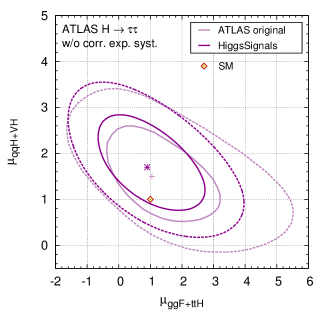
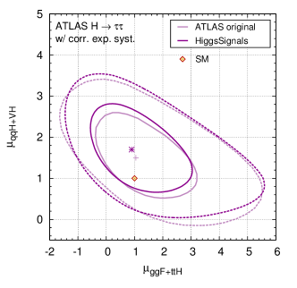
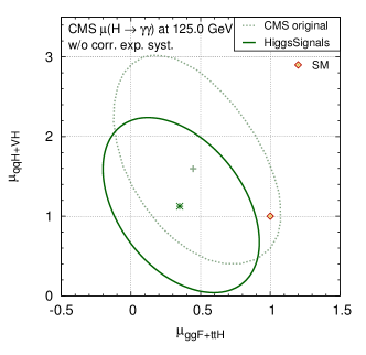
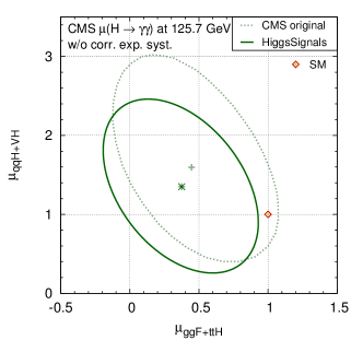
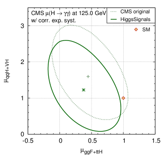
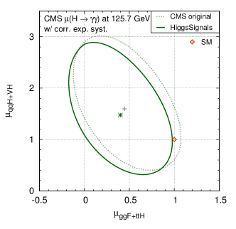
In earlier validation fits Bechtle:2013xfa using the CMS CMS:ril ; CMS:2012paa results we found some discrepancies if only a simple test was performed. In this case the correlations among these observables introduced by common sources of experimental systematic uncertainties are non-negligible. Guided by the information given in Ref. CMS:ril , we therefore introduce the following correlations for the CMS category measurements:
-
•
Event migration of between neighboring untagged categories for each and ,
-
•
Event migration of between the loose and tight dijet category at ,
-
•
For the dijet categories, we include a dijet tagging efficiency uncertainty, corresponding to an anti-correlated uncertainty among the ggH and VBF channels, of and , respectively.
-
•
cut efficiency uncertainty in the selection at of for the ggH and VBF channels and for the , , channels, respectively.
One more complication arises because the signal rate measurements in the various categories of the analysis are only publicly available for a mass value of . On the contrary, Ref. CMS:yva provides only fit results at for the signal strengths
| (20) | |||
| (21) | |||
| (22) |
combining the untagged, dijet and remaining leptonic/missing energy categories, respectively. Furthermore, the official scale factor fit results given by CMS, which can be used to validate our implementation, see Sect. A.2, assume a Higgs mass of CMS:yva . Given the category measurements at (based on the MVA analysis), cf. Tab. 14, we repeat these fits with HiggsSignals to obtain
| (23) | |||
| (24) | |||
| (25) |
We approximate the unknown category measurements at by rescaling the category measurements at by the ratio of the corresponding combined fit results.
In Fig. 21 we show the effects of including the correlations of systematic experimental uncertainties and the rescaling of the category measurements to for a 2D fit to common scale factors for the gluon fusion and cross section, , and for the vector boson fusion and () cross sections, , using only results from the CMS analysis CMS:2012paa ; CMS:ril . The original CMS result obtained for is overlaid in the figure. It can be seen that both effects have a sizable impact on the result. Acceptable agreement with the official CMS result can be obtained if both the correlations and the rescaling is taken into account, as shown in Fig. 21(d). We therefore use this setup of the CMS measurements for the fits presented in this paper.
A.2 Validation fit using CMS data only
We validate the fit procedure by performing a six-dimensional fit to the CMS Moriond 2013 data and comparing the results to the official fit results presented by CMS CMS:yva . The model parameters are identical to the scale factors of our general fit, i.e. , , , , and , but the total width is obtained from the rescaled effective couplings direcly (no additional Higgs decay modes). The CMS fit was performed assuming a Higgs boson mass of . The results are shown in Fig. 22, where the blue curves indicate the original CMS resultsCMS:yva . With the corrected implementation of the CMS measurements, as discussed above, the fit shows excellent agreement.
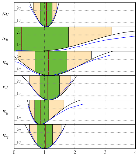
A.3 Projected sensitivity of future signal rate measurements
The future estimates of signal strength measurements in various channels at the LHC for integrated luminosities of and are given in Tab. 15 for ATLAS ATL-PHYS-PUB-2013-014 and CMS CMS:2013xfa . In Tab. 16 we list the estimated cross section and signal rate measurements at the ILC Asner:2013psa . These values are used for the study of the LHC and ILC capabilities of Higgs coupling determination presented in Sect. 4.
[b] Analysis C.L. precision Assumed signal composition [in %] ggH VBF WH ZH ATL ATL-PHYS-PUB-2013-014 ATL ATL-PHYS-PUB-2013-014 ATL ATL-PHYS-PUB-2013-014 ATL EuropeanStrategyforParticlePhysicsPreparatoryGroup:2013fia ATL EuropeanStrategyforParticlePhysicsPreparatoryGroup:2013fia ATL ATL-PHYS-PUB-2013-014 ATL ATL-PHYS-PUB-2013-014 ATL EuropeanStrategyforParticlePhysicsPreparatoryGroup:2013fia ATL ATL-PHYS-PUB-2013-014 ATL ATL-PHYS-PUB-2013-014 ATL ATL-PHYS-PUB-2013-014 ATL ATL-PHYS-PUB-2013-014 ATL ATL-PHYS-PUB-2013-014 ATL ATL-PHYS-PUB-2013-014 ATL EuropeanStrategyforParticlePhysicsPreparatoryGroup:2013fia ATL ATL-PHYS-PUB-2013-014 CMS CMS:2013xfa CMS CMS:2013xfa CMS CMS:2013xfa CMS CMS:2013xfa CMS CMS:2013xfa CMS CMS:2013xfa CMS CMS:2013xfa
| and | at | at | at | ||||
| - | - | - | - | - | |||
| - | - | - | - | - | - | ||
| mode | |||||||
| - | - | - | |||||
| - | - | - | |||||
| - | - | - | |||||
| - | - | - | |||||
| - | - | - | |||||
| - | - | - | |||||
| - | - | - | - | - | |||
| and | at | at | at | ||||
| - | - | - | - | - | |||
| - | - | - | - | - | - | ||
| mode | |||||||
| - | - | - | |||||
| - | - | - | |||||
| - | - | - | |||||
| - | - | - | |||||
| - | - | - | |||||
| - | - | - | |||||
| - | - | - | - | - | |||
Appendix B Investigating the -value of fits to measured Higgs signal rates
As outlined in Sect. 2.2 and explained in detail in Ref. Bechtle:2013xfa , HiggsSignals employs a approximation to allow for a very fast evaluation of the model compatibility with public results from Higgs rate and mass measurements in arbitrary models. Comparisons to the results from ATLAS and CMS show that this implementation yields a good approximation to the official results Bechtle:2013xfa (see also Appendices A.1 and A.2 above). This allows for a reliable phenomenological analysis of a very large variety of models of new physics against the Higgs search results. In such studies, the -value, i.e. the statistical agreement of the measured results with the predictions from a theory, is of high interest. This can be evaluated using toy Monte Carlo techniques. In this section we study to what extent the specific implementation of the evaluation in HiggsSignals impacts the -value calculation. This is also of interest for other implementations of tests against Higgs mass and rate measurements Lafaye:2009vr ; Klute:2012pu ; Plehn:2012iz ; Klute:2013cx ; Dobrescu:2012td ; Espinosa:2012im ; Cacciapaglia:2012wb ; Belanger:2012gc ; Ellis:2013lra ; Djouadi:2013qya ; Cheung:2013kla ; Holdom:2013axa ; Chpoi:2013wga ; Bechtle:2013xfa ; Belanger:2013xza ; Buckley:2012em ; Arbey:2012na ; Arbey:2012dq ; Akula:2012kk ; Cao:2012yn ; Howe:2012xe ; Drees:2012fb ; Haisch:2012re ; Bechtle:2012jw ; Arbey:2012bp ; Ke:2012zq ; Chakraborty:2013si ; Carmona:2013cq ; Arbey:2013jla ; Cao:2013wqa ; Bhattacherjee:2013vga ; Lopez-Val:2013yba ; Belyaev:2013ida ; Cao:2013gba ; Bharucha:2013ela ; Cheung:2013rva ; Bechtle:2013mda ; Cao:2013mqa ; Djouadi:2013lra ; Enberg:2013jba ; Cao:2013cfa ; Wang:2013sha ; Fan:2014txa ; Belanger:2014roa ; Stal:2014sua , which employ different levels of detail concerning the implementation of uncertainties (correlated/uncorrelated, relative/absolute, symmetric/asymmetric, etc.). In order to evaluate the impact of the calculation of uncertainties and correlations on the , we investigate the -value of a SM-like Higgs boson modified by a global scale parameter . It is tested against the latest rate measurements from ATLAS, CMS, CDF and DØ, see Appendix A for details. Using a toy Monte Carlo technique the -value is then evaluated from the HiggsSignals calculated for sets of pseudo-measurements thrown around the best fit point and according to the covariance matrix, which we obtain at the best fit point. The exact -value based on the full likelihood distribution can of course only be calculated by the experimental collaborations. However, no combination of the experiments at LHC and the Tevatron is available, such that an approximate calculation is of interest.
The default treatment of uncertainties in HiggsSignals suggests a deviation from the ideal distribution in both the signal strength part, , and the Higgs mass part, . Therefore, the -value can only approximately be extracted from the observed at the best fit point and the number of degrees of freedom (ndf) assuming an ideal distribution. Instead, toy measurements have to be employed to take into account the following effects in the -value evaluation:
-
1.
The usage of asymmetric (upper and lower) uncertainties in the rate measurements instead of averaged (symmetric) uncertainties. The choice for the observed rate uncertainty entering the evaluation, , is dependent on the relative position of the model-predicted signal rate with respect to the observed value :
(28) -
2.
The usage of relative instead of absolute rate uncertainties. The luminosity uncertainty is scaled with the observed value, while the theoretical rate uncertainties are scaled with the predicted value in HiggsSignals. Where the experimental systematics can not be attributed to either signal or background, they are treated as background-related and kept constant. This combination generally provides a good approximation of the experimental results.
In case that the mass is also fitted, two additional effects arise:
-
3.
Theoretical mass uncertainties can be treated as (anti-)correlated Gaussian errors in the evaluation. The theory mass uncertainty of two mass observables, , , is anti-correlated if the predicted mass lies in between these measurements, .
-
4.
The automatic assignment of the Higgs boson to the observables introduces a highly non-trivial deviation from the ideal shape in both and . This procedure takes care that the comparison of the predicted signal rate (at mass ) with the measured signal strength (at mass ) is still approximately valid, or otherwise adds a penalty to . In the latter case, the mass measurement associated with the unassigned observable does not enter anymore. This issue is of course only relevant if a model with more than one Higgs boson is studied. It is not further studied in the examples below.
The items (1, 2) lead to a dependence of the covariance matrix in the calculation on both the observed signal rate values, , and the model-predicted signal rate values, . Hence, it changes for each set of pseudo-measurements and depends on the tested model. The items (3, 4) are of relevance only in the case of a non-trivial model prediction of the Higgs mass. Here, we choose a fixed Higgs mass of . We ensure a full assignment of all observables within HiggsSignals, while the actual constant contribution from the Higgs mass measurements is of no further relevance in this study. It should be noted, however, that we hereby make the approximation/assumption, that all signal rates measured by the experiments for the Higgs signal at various mass positions between and can be compared with the hypothesized Higgs state at .
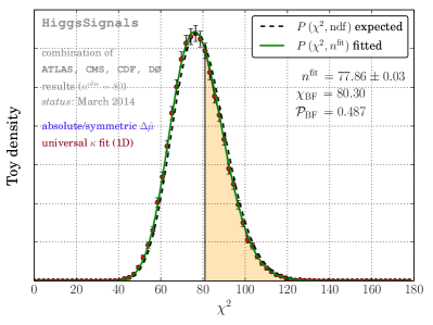
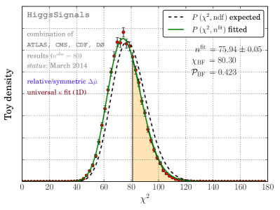
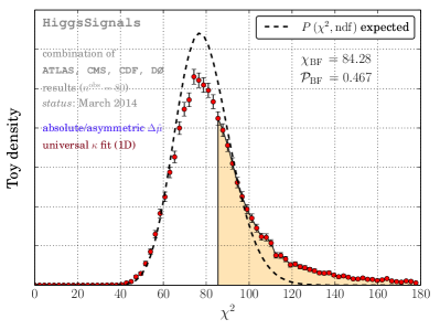
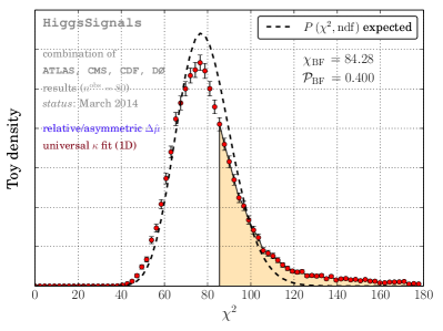
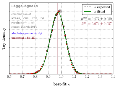
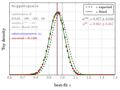
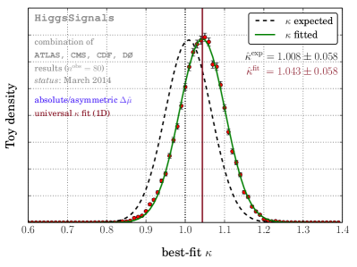
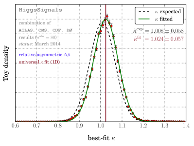
As a simple generic toy model we employ a fit with only one free parameter, namely a global Higgs coupling scale factor affecting all Higgs couplings to bosons and fermions in the same way, thus the SM predictions for the Higgs boson signal rates are universally scaled by . The toy data is created using the covariance matrix constructed under the principles outlined above and evaluated at the best fit point. The resulting distributions of the minimal from the toy experiments thrown around the best fit point in is shown in Fig. 23. In Fig. 23 (a), the main effects leading to a deviation from the naive -distribution are deactivated: Absolute rate uncertainties are used instead of relative ones for all statistical and systematic errors, and the experimental uncertainties are symmetrized. As expected, a nearly perfect shape is obtained. The original best fit point is located at with . The -value is given by the area under the obtained distribution for . In this treatment we obtain , indicating very good agreement of all Higgs rate measurements with the toy model chosen here. Note, that the best fit point is extremely close to the SM (with ), which features a in this treatment and thus a very similar -value.
The more realistic treatment of the uncertainties, however, has significant impact on the -value, as shown in Fig. 23(d). The full model dependence of the covariance matrix is used including relative errors and asymmetric experimental uncertainties. This is the most accurate approximation to the real likelihood distribution and thus provides a more accurate guess of the -value than the naive calculation above, where these effects have been ignored. The result differs from the previously obtained . More importantly, the shape of the histogram of the obtained values from the toy fits does not follow an ideal distribution anymore. More toy outcomes accumulate in the tail of the distribution at larger values, thus leading to a slightly improved -value of the original best fit point than expected when assuming an ideal shape. Toy MC studies like this will be of greater importance once the data is more precise, and in particular if significant deviations between the SM and the data emerge. analyses that do not take into account the effects described above might thus lead to conclusion significantly deviating from the full results.
In order to show the origin of the deviation of the -value from the idealized implementation, Fig. 23(a), the two major effects yielding deviations from the naive expectation are singled out in Fig. 23(b) and (c). In Fig. 23(b), only the effect of relative errors, cf. item (2) above, is applied while the uncertainties are kept symmetrized. It can be seen that the treatment of relative uncertainties by itself has rather small effects. This is because the preferred range of the global scale factor is with already quite narrow. Hence, varies only in a small range and the impact from uncertainties varying with is rather insignificant. However, the picture will change in more complex models with more freedom in the variation of individual rates, including some of the benchmark scale factor fits that are discussed in Sect. 3.
In Fig. 23(c) the effect of asymmetric errors, cf. item (1) above, is studied. In this case we hold the values of the uncertainties fixed for every toy measurement (absolute uncertainties). It can be seen that for the -value this effect fully dominates the full implementation in Fig. 23(d) and should not be omitted in any implementation, since it could have a significant effect on the conclusion.
In Fig. 24 we show the toy distribution of the best fit global scale factor for the four different settings discussed above. Again, Fig. 24(a) shows the idealized result with absolute and symmetrized uncertainties and (d) shows the result from the full implementation of relative and asymmetric uncertainties. The same variations as explained for the -value can also be observed in the distribution of the best fit points. A small negative bias of about in the universal coupling scale factor estimator is introduced by the relative uncertainties, as can be seen in Fig. 24(b). A much larger positive bias of the order of , however, results from the correct treatment of asymmetric errors, cf. Fig. 24 (c). This stems from the fact that the experimental uncertainties are typically larger for variations in the upward direction as a direct consequence of the likelihood shape. As expected the full result in Fig. 24(d) is in between (b) and (c) since both biases apply, leading to an upward shift between expected and fitted universal scale factor of . Note also, that the best-fit distribution happens to be systematically slightly narrower than what is expected from the naive comparison, but in this case by only , which corresponds to a change of only . We thus conclude that the Gaussian shape of the uncertainties is approximately preserved, and that the uncertainties derived from the profile likelihood in the main part of this paper are expected to be reliable estimates of the uncertainties obtained in a full MC toy based treatment, or even the full likelihood analysis in the experimental collaborations.
In summary, this simple toy model study shows that there are potentially significant effects affecting the evaluation of -values of arbitrary Higgs models tested against the signal rate measurements. These effects stem from non-Gaussian likelihood effects such as asymmetric uncertainties as well as different scaling behavior of systematic uncertainties with either the measured or predicted rates. Both effects are approximately accounted for in the evaluation in HiggsSignals, leading to an outcome that does not strictly follow the naive expectation of an ideal probability distribution with due to visible changes in the probability density function. In a detailed evaluation of the -value we therefore advice to take these effects into account by using toy experiments.
Appendix C Theoretical uncertainties of Higgs production and decay modes
The (correlated) uncertainties of the Higgs production and decay rates induced by the dependence on (common) parameters are evaluated as follows. We introduce a random variable following a Normal distribution,
| (29) |
for each common parametric dependence . In particular, the following common parametric dependencies are of relevance:
-
•
for the partial width uncertainties of all Higgs decay modes,
-
•
for the ggH and cross section uncertainties,
The smearing of the common parameter, described by , thus affects the resulting uncertainties of the corresponding production or decay modes in a fully correlated way (see also below). For the remaining parametric dependencies , individual Normal-distributed random variables are introduced per production or decay mode , thus these uncertainty sources are regarded as uncorrelated. Similarly, the theoretical uncertainties corresponding to estimates of the missing higher-order corrections are described by individual (and thus uncorrelated) Normal-distributed variations, , except in the case of and production which are treated as fully correlated.
In Eq. (29), is introduced as an artificial scale factor of the standard deviation of the parametric uncertainties. Usually, we choose , corresponding to a interpretation of the quoted uncertainties. For comparison, however, we define the setting ‘LHCHXSWG-matched’, where we adjust for the cross section [partial width] uncertainties in order to approximately match with the uncertainty estimates given by the LHCHXSWG. Note that all (theoretical, correlated or uncorrelated parametric) variations are described by Eq. (29), hence, for simplicity, the scale factor affects all variations in the same way.
[b] Mode LHCHXSWG1 LHCHXSWG LHC-S1 LHC-S2 ILC from Ref. Heinemeyer:2013tqa matched2 (ggH) - (VBF) - - - - - - - - - - - - - - - - Using a Gaussian-shaped parameter variation
-
1
Taken from Ref. Heinemeyer:2013tqa , using (always the larger) uncertainty estimates for , . Theoretical and parametric uncertainties are added linearly. In our naive fit, we use these numbers as maximum error estimates and neglect all correlations of common parametric uncertainty sources, total width, etc..
-
2
Using an artificially enlarged range for the parametric variation of and for the production cross section and partial width uncertainties, respectively.
We now employ a Monte-Carlo (MC) calculation, where each iteration (also called “toy”) is defined by throwing random numbers for the parametric and theoretical uncertainty variations, . Then, the production cross sections and partial widths predicted for this toy are evaluated as
| (30) | ||||
| (31) |
where and are the central values of the production cross sections and partial widths in the SM, respectively, and and their parametric or theoretical uncertainties as given in Ref. Heinemeyer:2013tqa . We take into account possibly asymmetric uncertainties:
| (34) |
Note, that and can also be negative, depending on the response of the calculated quantity to the parameter variation. From the partial widths we can simply derive for each toy the total decay width, , and branching ratios, . The covariance matrices are then given by
| (35) |
where denotes the arithmetic mean for the full toy MC sample and or .
In Tab. 17 we give the relative uncorrelated uncertainties, given by , for the LHC production cross sections and Higgs branching ratios for the future scenarios ‘LHC-S1’, ‘LHC-S2’ and ‘ILC’ discussed in Tab. 9. These are compared with the uncertainty estimates given by the LHCHXSWG Heinemeyer:2013tqa , where the parametric and theoretical uncertainties for a Higgs mass of and a center-of-mass energy of are added linearly. For the scenario ‘LHCHXSWG-matched’ we employ the toy MC procedure with the artificial scale factor and for the uncertainties of the production cross sections and branching ratios, respectively. We furthermore compared these uncertainty estimates with those obtained when using a uniform (box-shaped) smearing of the parametric and theoretical uncertainties instead of Eq. (29). The deviations found are rather small, being typically .
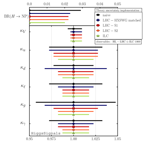
In order to investigate the impact of the different theoretical uncertainty implementations on the precision estimates of the Higgs coupling scale factors we perform the seven-dimensional scale factor fit, cf. Sect. 3.6 and 4.1, to the same combined future projections for the high-luminosity LHC and all baseline ILC stages up to , , for all implementations. The result is shown in Fig. 25. Comparing the ‘naive’ implementation, where simply the estimates from the LHCHXSWG are taken (cf. Tab. 17) and all correlations among the cross section and branching ratio predictions are neglected, with the ‘LHC-HXSWG matched’ implementation, we see that for the latter, and all scale factors except can be determined more precisely. Note, however, that the major effect causing these differences is actually the remaining mismatch of the uncertainty estimates, cf. Tab. 17, and not the inclusion of correlations. Nevertheless, as we have argued in this work, we find it more consistent to evaluate the covariances of the cross section and branching ratio predictions directly via the toy MC outlined above, leading to the uncertainty estimates denoted by ‘LHC-S1’. Here, we find the largest differences to the ‘naive’ implementation in the achievable precisions of , , and , being . As expected, in the scenarios with improved theoretical uncertainties the Higgs coupling precision is further improved, indicating that in this high-statistics scenario the theoretical uncertainties are a dominant limiting factor for the achievable precision.
References
- (1) ATLAS Collaboration, Observation of a new particle in the search for the Standard Model Higgs boson with the ATLAS detector at the LHC, Phys. Lett. B 716 (2012) 1, [arXiv:1207.7214].
- (2) CMS Collaboration, Observation of a new boson at a mass of 125 GeV with the CMS experiment at the LHC, Phys. Lett. B 716 (2012) 30, [arXiv:1207.7235].
- (3) ATLAS Collaboration, Combined coupling measurements of the Higgs-like boson with the ATLAS detector using up to 25 fb-1 of proton-proton collision data, ATLAS-CONF-2013-034, ATLAS-COM-CONF-2013-035.
- (4) ATLAS Collaboration, Study of the spin of the new boson with up to 25 fb-1 of ATLAS data, ATLAS-CONF-2013-040, ATLAS-COM-CONF-2013-048.
- (5) CMS Collaboration, Combination of standard model Higgs boson searches and measurements of the properties of the new boson with a mass near 125 GeV, CMS-PAS-HIG-13-005.
- (6) CMS Collaboration, Properties of the observed Higgs-like resonance using the diphoton channel, CMS-PAS-HIG-13-016.
- (7) CDF and DØ Collaborations, Higgs Boson Studies at the Tevatron, Phys. Rev. D 88 (2013) 052014, [arXiv:1303.6346].
- (8) A. David, A. Denner, M. Duehrssen, M. Grazzini, et al., LHC HXSWG interim recommendations to explore the coupling structure of a Higgs-like particle, arXiv:1209.0040.
- (9) S. Heinemeyer et al., Handbook of LHC Higgs Cross Sections: 3. Higgs Properties, arXiv:1307.1347.
- (10) D. Zeppenfeld, R. Kinnunen, A. Nikitenko, and E. Richter-Was, Measuring Higgs boson couplings at the CERN LHC, Phys. Rev. D 62 (2000) 013009, [hep-ph/0002036].
- (11) M. Duhrssen, Prospects for the measurement of Higgs boson coupling parameters in the mass range from 110–190 GeV, ATL-PHYS-2003-030.
- (12) M. Duhrssen, S. Heinemeyer, H. Logan, D. Rainwater, G. Weiglein, et al., Extracting Higgs boson couplings from CERN LHC data, Phys. Rev. D 70 (2004) 113009, [hep-ph/0406323].
- (13) M. Duhrssen, S. Heinemeyer, H. Logan, D. Rainwater, G. Weiglein, et al., Determination of Higgs-boson couplings at the LHC, hep-ph/0407190.
- (14) R. Lafaye, T. Plehn, M. Rauch, D. Zerwas, and M. Duhrssen, Measuring the Higgs Sector, JHEP 0908 (2009) 009, [arXiv:0904.3866].
- (15) M. Klute, R. Lafaye, T. Plehn, M. Rauch, and D. Zerwas, Measuring Higgs Couplings from LHC Data, Phys. Rev. Lett. 109 (2012) 101801, [arXiv:1205.2699].
- (16) T. Plehn and M. Rauch, Higgs Couplings after the Discovery, Europhys. Lett. 100 (2012) 11002, [arXiv:1207.6108].
- (17) M. Klute, R. Lafaye, T. Plehn, M. Rauch, and D. Zerwas, Measuring Higgs Couplings at a Linear Collider, Europhys. Lett. 101 (2013) 51001, [arXiv:1301.1322].
- (18) B. A. Dobrescu and J. D. Lykken, Coupling spans of the Higgs-like boson, JHEP 1302 (2013) 073, [arXiv:1210.3342].
- (19) J. Espinosa, C. Grojean, M. Mühlleitner, and M. Trott, First Glimpses at Higgs’ face, JHEP 1212 (2012) 045, [arXiv:1207.1717].
- (20) G. Cacciapaglia, A. Deandrea, G. D. La Rochelle, and J.-B. Flament, Higgs couplings beyond the Standard Model, JHEP 1303 (2013) 029, [arXiv:1210.8120].
- (21) G. Belanger, B. Dumont, U. Ellwanger, J. Gunion, and S. Kraml, Higgs Couplings at the End of 2012, JHEP 1302 (2013) 053, [arXiv:1212.5244].
- (22) J. Ellis and T. You, Updated Global Analysis of Higgs Couplings, JHEP 1306 (2013) 103, [arXiv:1303.3879].
- (23) A. Djouadi and G. Moreau, The couplings of the Higgs boson and its CP properties from fits of the signal strengths and their ratios at the 7+8 TeV LHC, arXiv:1303.6591.
- (24) K. Cheung, J. S. Lee, and P.-Y. Tseng, Higgs Precision (Higgcision) Era begins, JHEP 1305 (2013) 134, [arXiv:1302.3794].
- (25) B. Holdom, Far from standard Higgs couplings, arXiv:1306.1564.
- (26) S. Choi, S. Jung, and P. Ko, Implications of LHC data on 125 GeV Higgs-like boson for the Standard Model and its various extensions, JHEP 1310 (2013) 225, [arXiv:1307.3948].
- (27) P. Bechtle, S. Heinemeyer, O. Stål, T. Stefaniak, and G. Weiglein, HiggsSignals: Confronting arbitrary Higgs sectors with measurements at the Tevatron and the LHC, Eur. Phys. J. C 74 (2013) 2711, [arXiv:1305.1933].
- (28) G. Belanger, B. Dumont, U. Ellwanger, J. Gunion, and S. Kraml, Global fit to Higgs signal strengths and couplings and implications for extended Higgs sectors, Phys. Rev. D 88 (2013) 075008, [arXiv:1306.2941].
- (29) F. Caola and K. Melnikov, Constraining the Higgs boson width with ZZ production at the LHC, Phys. Rev. D 88 (2013) 054024, [arXiv:1307.4935].
- (30) J. M. Campbell, R. K. Ellis, and C. Williams, Gluon-Gluon Contributions to W+ W- Production and Higgs Interference Effects, JHEP 1110 (2011) 005, [arXiv:1107.5569].
- (31) J. M. Campbell, R. K. Ellis, and C. Williams, Bounding the Higgs width at the LHC: complementary results from , arXiv:1312.1628.
- (32) J. M. Campbell, R. K. Ellis, and C. Williams, Bounding the Higgs width at the LHC using full analytic results for , arXiv:1311.3589.
- (33) L. J. Dixon and Y. Li, Bounding the Higgs Boson Width Through Interferometry, Phys. Rev. Lett. 111 (2013) 111802, [arXiv:1305.3854].
- (34) M. R. Buckley and D. Hooper, Are There Hints of Light Stops in Recent Higgs Search Results?, Phys. Rev. D 86 (2012) 075008, [arXiv:1207.1445].
- (35) A. Arbey, M. Battaglia, and F. Mahmoudi, Light Neutralino Dark Matter in the pMSSM: Implications of LEP, LHC and Dark Matter Searches on SUSY Particle Spectra, Eur. Phys. J. C 72 (2012) 2169, [arXiv:1205.2557].
- (36) A. Arbey, M. Battaglia, A. Djouadi, and F. Mahmoudi, The Higgs sector of the phenomenological MSSM in the light of the Higgs boson discovery, JHEP 1209 (2012) 107, [arXiv:1207.1348].
- (37) S. Akula, P. Nath, and G. Peim, Implications of the Higgs Boson Discovery for mSUGRA, Phys. Lett. B 717 (2012) 188, [arXiv:1207.1839].
- (38) J. Cao, Z. Heng, J. M. Yang, and J. Zhu, Status of low energy SUSY models confronted with the LHC 125 GeV Higgs data, JHEP 1210 (2012) 079, [arXiv:1207.3698].
- (39) K. Howe and P. Saraswat, Excess Higgs Production in Neutralino Decays, JHEP 1210 (2012) 065, [arXiv:1208.1542].
- (40) M. Drees, A Supersymmetric Explanation of the Excess of Higgs–Like Events at the LHC and at LEP, Phys. Rev. D 86 (2012) 115018, [arXiv:1210.6507].
- (41) U. Haisch and F. Mahmoudi, MSSM: Cornered and Correlated, JHEP 1301 (2013) 061, [arXiv:1210.7806].
- (42) P. Bechtle, S. Heinemeyer, O. Stål, T. Stefaniak, G. Weiglein, and L. Zeune, MSSM Interpretations of the LHC Discovery: Light or Heavy Higgs?, Eur. Phys. J. C 73 (2013) 2354, [arXiv:1211.1955].
- (43) A. Arbey, M. Battaglia, A. Djouadi, and F. Mahmoudi, An update on the constraints on the phenomenological MSSM from the new LHC Higgs results, Phys. Lett. B 720 (2013) 153, [arXiv:1211.4004].
- (44) J. Ke, H. Luo, M.-x. Luo, K. Wang, L. Wang, et al., Revisit to Non-decoupling MSSM, Phys. Lett. B 723 (2013) 113, [arXiv:1211.2427].
- (45) A. Chakraborty, B. Das, J. L. Diaz-Cruz, D. K. Ghosh, S. Moretti, et al., The 125 GeV Higgs signal at the LHC in the CP Violating MSSM, arXiv:1301.2745.
- (46) A. Carmona and F. Goertz, Custodial Leptons and Higgs Decays, JHEP 1304 (2013) 163, [arXiv:1301.5856].
- (47) A. Arbey, M. Battaglia, and F. Mahmoudi, Supersymmetric Heavy Higgs Bosons at the LHC, Phys. Rev. D 88 (2013) 015007, [arXiv:1303.7450].
- (48) J. Cao, P. Wan, J. M. Yang, and J. Zhu, The SM extension with color-octet scalars: diphoton enhancement and global fit of LHC Higgs data, JHEP 1308 (2013) 009, [arXiv:1303.2426].
- (49) B. Bhattacherjee, M. Chakraborti, A. Chakraborty, U. Chattopadhyay, D. Das, et al., Implications of 98 GeV and 125 GeV Higgs scenario in non-decoupling SUSY with updated ATLAS, CMS and PLANCK data, Phys. Rev. D 88 (2013) 035011, [arXiv:1305.4020].
- (50) D. Lopez-Val, T. Plehn, and M. Rauch, Measuring extended Higgs sectors as a consistent free couplings model, JHEP 1310 (2013) 134, [arXiv:1308.1979].
- (51) A. Belyaev, M. S. Brown, R. Foadi, and M. T. Frandsen, The Technicolor Higgs in the Light of LHC Data, arXiv:1309.2097.
- (52) J. Cao, F. Ding, C. Han, J. M. Yang, and J. Zhu, A light Higgs scalar in the NMSSM confronted with the latest LHC Higgs data, JHEP 1311 (2013) 018, [arXiv:1309.4939].
- (53) A. Bharucha, A. Goudelis, and M. McGarrie, En-gauging Naturalness, arXiv:1310.4500.
- (54) K. Cheung, J. S. Lee, and P.-Y. Tseng, Higgcision in the Two-Higgs Doublet Models, JHEP 1401 (2014) 085, [arXiv:1310.3937].
- (55) P. Bechtle, K. Desch, H. K. Dreiner, M. Hamer, M. Krämer, et al., Constrained Supersymmetry after the Higgs Boson Discovery: A global analysis with Fittino, arXiv:1310.3045.
- (56) J. Cao, C. Han, L. Wu, P. Wu, and J. M. Yang, A light SUSY dark matter after CDMS-II, LUX and LHC Higgs data, arXiv:1311.0678.
- (57) A. Djouadi, Implications of the Higgs discovery for the MSSM, arXiv:1311.0720.
- (58) R. Enberg, J. Rathsman, and G. Wouda, Higgs phenomenology in the Stealth Doublet Model, arXiv:1311.4367.
- (59) J. Cao, Y. He, P. Wu, M. Zhang, and J. Zhu, Higgs Phenomenology in the Minimal Dilaton Model after Run I of the LHC, JHEP 1401 (2014) 150, [arXiv:1311.6661].
- (60) L. Wang and X.-F. Han, Status of the aligned two-Higgs-doublet model confronted with the Higgs data, arXiv:1312.4759.
- (61) J. Fan and M. Reece, A New Look at Higgs Constraints on Stops, arXiv:1401.7671.
- (62) G. Belanger, V. Bizouard, and G. Chalons, Boosting Higgs decays into gamma and a Z in the NMSSM, arXiv:1402.3522.
- (63) O. Stål, Prospects for Higgs boson scenarios beyond the Standard Model, arXiv:1402.6732.
- (64) O. Stål and T. Stefaniak, Constraining extended Higgs sectors with HiggsSignals, PoS EPS-HEP (2013) 314, [arXiv:1310.4039].
- (65) J. M. Cornwall, D. N. Levin, and G. Tiktopoulos, Uniqueness of spontaneously broken gauge theories, Phys. Rev. Lett. 30 (1973) 1268.
- (66) C. Llewellyn Smith, High-Energy Behavior and Gauge Symmetry, Phys. Lett. B 46 (1973) 233.
- (67) S. Dittmaier et al., Handbook of LHC Higgs Cross Sections: 1. Inclusive Observables, arXiv:1101.0593.
- (68) S. Dittmaier et al., Handbook of LHC Higgs Cross Sections: 2. Differential Distributions, arXiv:1201.3084.
- (69) R. V. Harlander, S. Liebler, and T. Zirke, Higgs Strahlung at the Large Hadron Collider in the 2-Higgs-Doublet Model, arXiv:1307.8122.
- (70) O. J. Eboli and D. Zeppenfeld, Observing an invisible Higgs boson, Phys.Lett. B495 (2000) 147–154, [hep-ph/0009158].
- (71) P. Bechtle, O. Brein, S. Heinemeyer, G. Weiglein, and K. E. Williams, HiggsBounds: Confronting Arbitrary Higgs Sectors with Exclusion Bounds from LEP and the Tevatron, Comput. Phys. Commun. 181 (2010) 138, [arXiv:0811.4169].
- (72) P. Bechtle, O. Brein, S. Heinemeyer, G. Weiglein, and K. E. Williams, HiggsBounds 2.0.0: Confronting Neutral and Charged Higgs Sector Predictions with Exclusion Bounds from LEP and the Tevatron, Comput. Phys. Commun. 182 (2011) 2605, [arXiv:1102.1898].
- (73) P. Bechtle, O. Brein, S. Heinemeyer, O. Stål, T. Stefaniak, et al., Recent Developments in HiggsBounds and a Preview of HiggsSignals, PoS CHARGED2012 (2012) 024, [arXiv:1301.2345].
- (74) P. Bechtle, O. Brein, S. Heinemeyer, O. Stål, T. Stefaniak, et al., HiggsBounds-4: Improved Tests of Extended Higgs Sectors against Exclusion Bounds from LEP, the Tevatron and the LHC, Eur. Phys. J. C 74 (2013) 2693, [arXiv:1311.0055].
- (75) S. Banerjee, S. Mukhopadhyay, and B. Mukhopadhyaya, Higher dimensional operators and LHC Higgs data : the role of modified kinematics, arXiv:1308.4860.
- (76) I. Anderson, S. Bolognesi, F. Caola, Y. Gao, A. V. Gritsan, et al., Constraining anomalous HVV interactions at proton and lepton colliders, arXiv:1309.4819.
- (77) A. Azatov and A. Paul, Probing Higgs couplings with high Higgs production, arXiv:1309.5273.
- (78) E. Boos, V. Bunichev, M. Dubinin, and Y. Kurihara, Higgs boson signal at complete tree level in the SM extension by dimension-six operators, arXiv:1309.5410.
- (79) M. Chen, T. Cheng, J. S. Gainer, A. Korytov, K. T. Matchev, et al., The role of interference in unraveling the ZZ-couplings of the newly discovered boson at the LHC, arXiv:1310.1397.
- (80) G. Buchalla, O. Cata, and G. D’Ambrosio, Nonstandard Higgs Couplings from Angular Distributions in , arXiv:1310.2574.
- (81) B. Dumont, S. Fichet, and G. von Gersdorff, A Bayesian view of the Higgs sector with higher dimensional operators, JHEP 1307 (2013) 065, [arXiv:1304.3369].
- (82) W. Buchmüller and D. Wyler, Effective Lagrangian Analysis of New Interactions and Flavor Conservation, Nucl. Phys. B 268 (1986) 621.
- (83) R. Contino, M. Ghezzi, C. Grojean, M. Mühlleitner, and M. Spira, Effective Lagrangian for a light Higgs-like scalar, JHEP 1307 (2013) 035, [arXiv:1303.3876].
- (84) A. Pomarol and F. Riva, Towards the Ultimate SM Fit to Close in on Higgs Physics, JHEP 1401 (2014) 151, [arXiv:1308.2803].
- (85) F. Boudjema, G. Cacciapaglia, K. Cranmer, G. Dissertori, A. Deandrea, et al., On the presentation of the LHC Higgs Results, arXiv:1307.5865.
- (86) CMS Collaboration, Updated measurements of the Higgs boson at 125 GeV in the two photon decay channel, CMS-PAS-HIG-13-001.
- (87) ATLAS Collaboration, Evidence for Higgs Boson Decays to the Final State with the ATLAS Detector, ATLAS-CONF-2013-108, ATLAS-COM-CONF-2013-095.
- (88) P. Bechtle and T. Stefaniak, “On the presentation of correlated systematic uncertainties in Higgs boson rate measurements.” available online at http://higgsbounds.hepforge.org.
- (89) K. Cranmer, S. Kreiss, D. Lopez-Val, and T. Plehn, A Novel Approach to Higgs Coupling Measurements, arXiv:1401.0080.
- (90) H. Haario, E. Saksman, and J. Tamminen, An adaptive Metropolis algorithm, Bernoulli 7 (2001), no. 2 223.
- (91) A. Patil, D. Huard, and C. J. Fonnesbeck, PyMC: Bayesian Stochastic Modelling in Python, Journal of Statistical Software 35 (2010), no. 4 1.
- (92) P. Bechtle, S. Heinemeyer, O. Stål, T. Stefaniak, and G. Weiglein, “Release Note for HiggsSignals-1.1.” available online at http://higgsbounds.hepforge.org.
- (93) A. Denner, S. Heinemeyer, I. Puljak, D. Rebuzzi, and M. Spira, Standard Model Higgs-Boson Branching Ratios with Uncertainties, Eur. Phys. J. C 71 (2011) 1753, [arXiv:1107.5909].
- (94) CMS Collaboration, Measurement of the properties of a Higgs boson in the four-lepton final state, arXiv:1312.5353.
- (95) G. Belanger, B. Dumont, U. Ellwanger, J. Gunion, and S. Kraml, Status of invisible Higgs decays, Phys. Lett. B 723 (2013) 340–347, [arXiv:1302.5694].
- (96) J. M. Cline, K. Kainulainen, P. Scott, and C. Weniger, Update on scalar singlet dark matter, Phys. Rev. D 88 (2013) 055025, [arXiv:1306.4710].
- (97) H. K. Dreiner, An Introduction to explicit R-parity violation, hep-ph/9707435.
- (98) R. Barbier, C. Berat, M. Besancon, M. Chemtob, A. Deandrea, et al., R-parity violating supersymmetry, Phys. Rept. 420 (2005) 1, [hep-ph/0406039].
- (99) H. Georgi and M. Machacek, DOUBLY CHARGED HIGGS BOSONS, Nucl. Phys. B 262 (1985) 463.
- (100) M. S. Chanowitz and M. Golden, Higgs Boson Triplets With M () = M () , Phys. Lett. B 165 (1985) 105.
- (101) J. Gunion, R. Vega, and J. Wudka, Higgs triplets in the standard model, Phys. Rev. D 42 (1990) 1673.
- (102) S. Chang, A ’Littlest Higgs’ model with custodial SU(2) symmetry, JHEP 0312 (2003) 057, [hep-ph/0306034].
- (103) A. Falkowski, S. Rychkov, and A. Urbano, What if the Higgs couplings to W and Z bosons are larger than in the Standard Model?, JHEP 1204 (2012) 073, [arXiv:1202.1532].
- (104) S. Chang, C. A. Newby, N. Raj, and C. Wanotayaroj, Revisiting Theories with Enhanced Higgs Couplings to Weak Gauge Bosons, Phys. Rev. D 86 (2012) 095015, [arXiv:1207.0493].
- (105) J. Hisano and K. Tsumura, Higgs boson mixes with an SU(2) septet representation, Phys. Rev. D 87 (2013) 053004, [arXiv:1301.6455].
- (106) S. Kanemura, M. Kikuchi, and K. Yagyu, Probing exotic Higgs sectors from the precise measurement of Higgs boson couplings, Phys. Rev. D 88 (2013) 015020, [arXiv:1301.7303].
- (107) ATLAS Collaboration, Search for invisible decays of a Higgs boson produced in association with a Z boson in ATLAS, ATLAS-CONF-2013-011, ATLAS-COM-CONF-2013-013.
- (108) CMS Collaboration, Search for invisible Higgs produced in association with a Z boson, CMS-PAS-HIG-13-018.
- (109) CMS Collaboration, Search for the Higgs boson decaying to invisible particles produced in association with Z bosons decaying to bottom quarks, CMS-PAS-HIG-13-028.
- (110) S. Heinemeyer, W. Hollik, and G. Weiglein, FeynHiggs: A Program for the calculation of the masses of the neutral CP even Higgs bosons in the MSSM, Comput. Phys. Commun. 124 (2000) 76, [hep-ph/9812320].
- (111) T. Hahn, S. Heinemeyer, W. Hollik, H. Rzehak, and G. Weiglein, FeynHiggs: A program for the calculation of MSSM Higgs-boson observables - Version 2.6.5, Comput. Phys. Commun. 180 (2009) 1426.
- (112) U. Aglietti, R. Bonciani, G. Degrassi, and A. Vicini, Analytic Results for Virtual QCD Corrections to Higgs Production and Decay, JHEP 0701 (2007) 021, [hep-ph/0611266].
- (113) R. Bonciani, G. Degrassi, and A. Vicini, Scalar particle contribution to Higgs production via gluon fusion at NLO, JHEP 0711 (2007) 095, [arXiv:0709.4227].
- (114) A. Djouadi, J. Kalinowski, and M. Spira, HDECAY: A Program for Higgs boson decays in the standard model and its supersymmetric extension, Comput. Phys. Commun. 108 (1998) 56, [hep-ph/9704448].
- (115) M. Spira, QCD effects in Higgs physics, Fortsch. Phys. 46 (1998) 203, [hep-ph/9705337].
- (116) R. Schabinger and J. D. Wells, A Minimal spontaneously broken hidden sector and its impact on Higgs boson physics at the large hadron collider, Phys. Rev. D 72 (2005) 093007, [hep-ph/0509209].
- (117) B. Patt and F. Wilczek, Higgs-field portal into hidden sectors, hep-ph/0605188.
- (118) V. Barger, P. Langacker, M. McCaskey, M. J. Ramsey-Musolf, and G. Shaughnessy, LHC Phenomenology of an Extended Standard Model with a Real Scalar Singlet, Phys. Rev. D 77 (2008) 035005, [arXiv:0706.4311].
- (119) V. Barger, P. Langacker, M. McCaskey, M. Ramsey-Musolf, and G. Shaughnessy, Complex Singlet Extension of the Standard Model, Phys. Rev. D 79 (2009) 015018, [arXiv:0811.0393].
- (120) G. Bhattacharyya, G. C. Branco, and S. Nandi, Universal Doublet-Singlet Higgs Couplings and phenomenology at the CERN Large Hadron Collider, Phys. Rev. D 77 (2008) 117701, [arXiv:0712.2693].
- (121) S. Bock, R. Lafaye, T. Plehn, M. Rauch, D. Zerwas, et al., Measuring Hidden Higgs and Strongly-Interacting Higgs Scenarios, Phys. Lett. B 694 (2010) 44, [arXiv:1007.2645].
- (122) C. Englert, T. Plehn, D. Zerwas, and P. M. Zerwas, Exploring the Higgs portal, Phys. Lett. B 703 (2011) 298, [arXiv:1106.3097].
- (123) C. Englert, T. Plehn, M. Rauch, D. Zerwas, and P. M. Zerwas, LHC: Standard Higgs and Hidden Higgs, Phys. Lett. B 707 (2012) 512, [arXiv:1112.3007].
- (124) G. M. Pruna and T. Robens, The Higgs Singlet extension parameter space in the light of the LHC discovery, Phys. Rev. D 88 (2013) 115012, [arXiv:1303.1150].
- (125) G. Giudice, C. Grojean, A. Pomarol, and R. Rattazzi, The Strongly-Interacting Light Higgs, JHEP 0706 (2007) 045, [hep-ph/0703164].
- (126) K. Agashe, R. Contino, and A. Pomarol, The Minimal composite Higgs model, Nucl. Phys. B 719 (2005) 165, [hep-ph/0412089].
- (127) R. Contino, L. Da Rold, and A. Pomarol, Light custodians in natural composite Higgs models, Phys. Rev. D 75 (2007) 055014, [hep-ph/0612048].
- (128) G. Altarelli and R. Barbieri, Vacuum polarization effects of new physics on electroweak processes, Phys. Lett. B 253 (1991) 161.
- (129) M. E. Peskin and T. Takeuchi, Estimation of oblique electroweak corrections, Phys. Rev. D 46 (1992) 381.
- (130) M. Baak, M. Goebel, J. Haller, A. Hoecker, D. Kennedy, et al., The Electroweak Fit of the Standard Model after the Discovery of a New Boson at the LHC, Eur. Phys. J. C 72 (2012) 2205, [arXiv:1209.2716].
- (131) M. Ciuchini, E. Franco, S. Mishima, and L. Silvestrini, Electroweak Precision Observables, New Physics and the Nature of a 126 GeV Higgs Boson, arXiv:1306.4644.
- (132) T. Lee, A Theory of Spontaneous T Violation, Phys. Rev. D 8 (1973) 1226.
- (133) S. L. Glashow and S. Weinberg, Natural Conservation Laws for Neutral Currents, Phys. Rev. D 15 (1977) 1958.
- (134) N. G. Deshpande and E. Ma, Pattern of Symmetry Breaking with Two Higgs Doublets, Phys. Rev. D 18 (1978) 2574.
- (135) J. F. Donoghue and L. F. Li, Properties of Charged Higgs Bosons, Phys. Rev. D 19 (1979) 945.
- (136) H. Haber, G. L. Kane, and T. Sterling, The Fermion Mass Scale and Possible Effects of Higgs Bosons on Experimental Observables, Nucl. Phys. B 161 (1979) 493.
- (137) L. J. Hall and M. B. Wise, FLAVOR CHANGING HIGGS - BOSON COUPLINGS, Nucl. Phys. B 187 (1981) 397.
- (138) J. F. Gunion and H. E. Haber, The CP conserving two Higgs doublet model: The Approach to the decoupling limit, Phys. Rev. D 67 (2003) 075019, [hep-ph/0207010].
- (139) G. Branco, P. Ferreira, L. Lavoura, M. Rebelo, M. Sher, et al., Theory and phenomenology of two-Higgs-doublet models, Phys. Rept. 516 (2012) 1, [arXiv:1106.0034].
- (140) T. Cheng and M. Sher, Mass Matrix Ansatz and Flavor Nonconservation in Models with Multiple Higgs Doublets, Phys. Rev. D 35 (1987) 3484.
- (141) H. E. Haber and G. L. Kane, The Search for Supersymmetry: Probing Physics Beyond the Standard Model, Phys. Rept. 117 (1985) 75–263.
- (142) J. Gunion and H. E. Haber, Higgs Bosons in Supersymmetric Models. 1., Nucl. Phys. B 272 (1986) 1.
- (143) J. Gunion and H. E. Haber, Higgs Bosons in Supersymmetric Models. 2. Implications for Phenomenology, Nucl. Phys. 278 (1986) 449.
- (144) J. F. Gunion, H. E. Haber, G. L. Kane, and S. Dawson, The Higgs Hunter’s Guide, Front. Phys. 80 (2000) 1.
- (145) F. Mahmoudi and O. Stål, Flavor constraints on the two-Higgs-doublet model with general Yukawa couplings, Phys. Rev. D 81 (2010) 035016, [arXiv:0907.1791].
- (146) A. Crivellin, C. Greub, and A. Kokulu, Explaining , and in a 2HDM of type III, Phys. Rev. D 86 (2012) 054014, [arXiv:1206.2634].
- (147) A. Crivellin, A. Kokulu, and C. Greub, Flavor-phenomenology of two-Higgs-doublet models with generic Yukawa structure, Phys. Rev. D 87 (2013) 094031, [arXiv:1303.5877].
- (148) R. Hempfling, Yukawa coupling unification with supersymmetric threshold corrections, Phys. Rev. D 49 (1994) 6168.
- (149) L. J. Hall, R. Rattazzi, and U. Sarid, The Top quark mass in supersymmetric SO(10) unification, Phys. Rev. D 50 (1994) 7048, [hep-ph/9306309].
- (150) M. S. Carena, M. Olechowski, S. Pokorski, and C. Wagner, Electroweak symmetry breaking and bottom - top Yukawa unification, Nucl. Phys. B 426 (1994) 269, [hep-ph/9402253].
- (151) CMS Collaboration, Search for the Standard-Model Higgs boson decaying to tau pairs in proton-proton collisions at sqrt(s) = 7 and 8 TeV, CMS-PAS-HIG-13-004. Updated results (dated Dec 2013) taken from TWiki page: https://twiki.cern.ch/twiki/bin/view/CMSPublic/Hig13004TWikiUpdate.
- (152) CMS Collaboration, Evidence for the 125 GeV Higgs boson decaying to a pair of leptons, arXiv:1401.5041.
- (153) CMS Collaboration, Evidence for the direct decay of the 125 GeV Higgs boson to fermions, arXiv:1401.6527.
- (154) M. Carena, S. Gori, N. R. Shah, and C. E. Wagner, A 125 GeV SM-like Higgs in the MSSM and the rate, JHEP 1203 (2012) 014, [arXiv:1112.3336].
- (155) M. Carena, S. Gori, N. R. Shah, C. E. Wagner, and L.-T. Wang, Light Stau Phenomenology and the Higgs Rate, JHEP 1207 (2012) 175, [arXiv:1205.5842].
- (156) L. Basso and F. Staub, Enhancing with staus in SUSY models with extended gauge sector, Phys. Rev. D 87 (2013) 015011, [arXiv:1210.7946].
- (157) M. Carena, S. Heinemeyer, O. Stål, C. Wagner, and G. Weiglein, MSSM Higgs Boson Searches at the LHC: Benchmark Scenarios after the Discovery of a Higgs-like Particle, Eur. Phys. J. C 73 (2013) 2552, [arXiv:1302.7033].
- (158) K. Schmidt-Hoberg and F. Staub, Enhanced rate in MSSM singlet extensions, JHEP 1210 (2012) 195, [arXiv:1208.1683].
- (159) M. Hemeda, S. Khalil, and S. Moretti, Light Chargino Effects onto in the MSSM, arXiv:1312.2504.
- (160) P. Posch, Enhancement of in the Two Higgs Doublet Model Type I, Phys. Lett. B 696 (2011) 447, [arXiv:1001.1759].
- (161) A. Drozd, B. Grzadkowski, J. F. Gunion, and Y. Jiang, Two-Higgs-Doublet Models and Enhanced Rates for a 125 GeV Higgs, JHEP 1305 (2013) 072, [arXiv:1211.3580].
- (162) A. Cordero-Cid, J. Hernandez-Sanchez, C. Honorato, S. Moretti, M. Perez, et al., Impact of a four-zero Yukawa texture on and in the framework of the 2-Higgs Doublet Model Type III, arXiv:1312.5614.
- (163) A. Arhrib, R. Benbrik, and N. Gaur, in Inert Higgs Doublet Model, Phys. Rev. D 85 (2012) 095021, [arXiv:1201.2644].
- (164) A. Goudelis, B. Herrmann, and O. Stål, Dark matter in the Inert Doublet Model after the discovery of a Higgs-like boson at the LHC, JHEP 1309 (2013) 106, [arXiv:1303.3010].
- (165) M. Krawczyk, D. Sokolowska, P. Swaczyna, and B. Swiezewska, Constraining Inert Dark Matter by and WMAP data, JHEP 1309 (2013) 055, [arXiv:1305.6266].
- (166) M. Krawczyk, D. Sokolowska, P. Swaczyna, and B. Swiezewska, Higgs , in the Inert Doublet Model, Acta Phys. Polon. B 44 (2013) 2163, [arXiv:1309.7880].
- (167) A. Djouadi, Squark effects on Higgs boson production and decay at the LHC, Phys. Lett. B 435 (1998) 101, [hep-ph/9806315].
- (168) M. S. Carena, S. Heinemeyer, C. Wagner, and G. Weiglein, Suggestions for benchmark scenarios for MSSM Higgs boson searches at hadron colliders, Eur. Phys. J. C 26 (2003) 601, [hep-ph/0202167].
- (169) CMS Collaboration, Search for the standard model Higgs boson produced in association with top quarks in multilepton final states, CMS-PAS-HIG-13-020.
- (170) CMS Collaboration, Search for Higgs Boson Production in Association with a Top-Quark Pair and Decaying to Bottom Quarks or Tau Leptons, CMS-PAS-HIG-13-019.
- (171) CMS Collaboration, Search for ttH production in events where H decays to photons at 8 TeV collisions, CMS-PAS-HIG-13-015.
- (172) CMS Collaboration, “Combination of search results for higgs boson production in association with a top-quark pair.” https://twiki.cern.ch/twiki/bin/view/CMSPublic/ttHCombinationTWiki.
- (173) R. Aleksan et al., Physics Briefing Book: Input for the Strategy Group to draft the update of the European Strategy for Particle Physics, .
- (174) ATLAS Collaboration, Physics at a High-Luminosity LHC with ATLAS, arXiv:1307.7292.
- (175) ATLAS Collaboration, Projections for measurements of Higgs boson cross sections, branching ratios and coupling parameters with the ATLAS detector at a HL-LHC, ATL-PHYS-PUB-2013-014.
- (176) CMS Collaboration, Projected Performance of an Upgraded CMS Detector at the LHC and HL-LHC: Contribution to the Snowmass Process, arXiv:1307.7135.
- (177) S. Dawson, A. Gritsan, H. Logan, J. Qian, C. Tully, et al., Higgs Working Group Report of the Snowmass 2013 Community Planning Study, arXiv:1310.8361.
- (178) M. E. Peskin, Estimation of LHC and ILC Capabilities for Precision Higgs Boson Coupling Measurements, arXiv:1312.4974.
- (179) D. Asner, T. Barklow, C. Calancha, K. Fujii, N. Graf, et al., ILC Higgs White Paper, arXiv:1310.0763.
- (180) J. Campbell, K. Hatakeyama, J. Huston, F. Petriello, J. R. Andersen, et al., Report of the Snowmass 2013 energy frontier QCD working group, arXiv:1310.5189.
- (181) H. Baer, T. Barklow, K. Fujii, Y. Gao, A. Hoang, et al., The International Linear Collider Technical Design Report - Volume 2: Physics, arXiv:1306.6352.
- (182) T. Han, Z. Liu, and J. Sayre, Potential Precision on Higgs Couplings and Total Width at the ILC, arXiv:1311.7155.
- (183) I. Campos et al., Phenomenology Tools on Cloud Infrastructures using OpenStack, Eur. Phys. J. C 73 (2013) 2375, [arXiv:1212.4784].
- (184) ATLAS Collaboration, Measurements of the properties of the Higgs-like boson in the decay channel with the ATLAS detector using 25 fb-1 of proton-proton collision data, ATLAS-CONF-2013-030, ATLAS-COM-CONF-2013-028.
- (185) ATLAS Collaboration, Measurements of Higgs boson production and couplings in diboson final states with the ATLAS detector at the LHC, Phys. Lett. B 726 (2013) 88, [arXiv:1307.1427].
- (186) ATLAS Collaboration, Measurements of the properties of the Higgs-like boson in the four lepton decay channel with the ATLAS detector using 25 fb?1 of proton-proton collision data, ATLAS-CONF-2013-013, ATLAS-COM-CONF-2013-018.
- (187) ATLAS Collaboration, Observation of an excess of events in the search for the Standard Model Higgs boson in the gamma-gamma channel with the ATLAS detector, ATLAS-CONF-2012-091, ATLAS-COM-CONF-2012-109.
- (188) ATLAS Collaboration, Measurements of the properties of the Higgs-like boson in the two photon decay channel with the ATLAS detector using 25 of proton-proton collision data, ATLAS-CONF-2013-012, ATLAS-COM-CONF-2013-015.
- (189) ATLAS collaboration, Search for the bb decay of the Standard Model Higgs boson in associated W/ZH production with the ATLAS detector, ATLAS-CONF-2013-079, ATLAS-COM-CONF-2013-080.
- (190) ATLAS Collaboration, Search for associated production of the Higgs boson in the and channels with the ATLAS detector at the LHC, ATLAS-CONF-2013-075, ATLAS-COM-CONF-2013-069.
- (191) CDF Collaboration, Combination of searches for the Higgs boson using the full CDF data set, Phys. Rev. D 88 (2013) 052013, [arXiv:1301.6668].
- (192) CMS Collaboration, Measurement of Higgs boson production and properties in the WW decay channel with leptonic final states, arXiv:1312.1129.
- (193) CMS Collaboration, VH with HWW and Vjj, CMS-PAS-HIG-13-017.
- (194) CMS Collaboration, Properties of the Higgs-like boson in the decay in collisions at and TeV, CMS-PAS-HIG-13-002.
- (195) CMS Collaboration, Evidence for a new state decaying into two photons in the search for the standard model Higgs boson in pp collisions, CMS-PAS-HIG-12-015.
- (196) CMS Collaboration, Search for the standard model Higgs boson in the dimuon decay channel in pp collisions at sqrt(s)= 7 and 8 TeV, CMS-PAS-HIG-13-007.
- (197) CMS Collaboration, Search for the standard model Higgs boson produced in association with W or Z bosons, and decaying to bottom quarks for LHCp 2013, CMS-PAS-HIG-13-012.
- (198) DØ Collaboration, Combined search for the Higgs boson with the D0 experiment, Phys. Rev. D 88 (2013) 052011, [arXiv:1303.0823].