Measuring and modeling correlations in multiplex networks

Abstract

The interactions among the elementary components of many complex systems can be qualitatively different. Such systems are therefore naturally described in terms of multiplex or multi-layer networks, i.e. networks where each layer stands for a different type of interaction between the same set of nodes. There is today a growing interest in understanding when and why a description in terms of a multiplex network is necessary and more informative than a single-layer projection. Here, we contribute to this debate by presenting a comprehensive study of correlations in multiplex networks. Correlations in node properties, especially degree-degree correlations, have been thoroughly studied in single-layer networks. Here we extend this idea to investigate and characterize correlations between the different layers of a multiplex network. Such correlations are intrinsically multiplex, and we first study them empirically by constructing and analyzing several multiplex networks from the real-world. In particular, we introduce various measures to characterize correlations in the activity of the nodes and in their degree at the different layers, and between activities and degrees. We show that real-world networks exhibit indeed non-trivial multiplex correlations. For instance, we find cases where two layers of the same multiplex network are positively correlated in terms of node degrees, while other two layers are negatively correlated. We then focus on constructing synthetic multiplex networks, proposing a series of models to reproduce the correlations observed empirically and/or to assess their relevance.

I Introduction

Since its origins, the new science of complex networks has been primarily driven by the need to characterize the properties of real-world systems Newman2003rev ; Boccaletti2006 . The introduction of new ideas and concepts in the field has been very often associated to the availability of new, more accurate, or larger data sets, and to the discovery of new structural properties of complex systems from the real world Watts1998 ; Barabasi1999 ; Amaral2000 ; Barrat2004 ; Pastor-Satorras2001 ; Vespignani2001 ; Latora2001 ; Newman2001c ; Newman2002 ; Girvan2002 . This is the reason why a lot of interest has been recently devoted to the study of multiplex networks, i.e. networks in which the same set of nodes can be connected by means of links of qualitatively different type or nature.

Several data sets of real-world systems that can be represented and studied as multiplex networks have appeared in the recent literature Szell2010 ; Cardillo2013_Emergence ; Cardillo2013_Airports ; Battiston2014 , and we expect that many more will arrive in the next few years. The first papers on the subject have focused on the characterization of the structure of multiplex networks DeDomenico2013_tensor ; DeDomenico2013_Centrality ; Menichetti2014 ; Battiston2014 ; Sola2013 ; Cozzo2013_Clustering ; Estrada2013 ; Corominas2013 ; Radicchi2013 ; Bianconi2014_component ; Bianconi2013 ; Halu2013 ; DeDomenico2015structural , and on modeling the basic mechanisms of their growth Nicosia2013 ; Kim2013 ; Nicosia2014 ; Klimek2013 ; Fotouhi2015 . In parallel to this, some effort has been also devoted on investigating various kinds of dynamical processes on multiplex topologies, including diffusion Gomez2013 ; DeDomenico2013_RW ; Sole2013_Spectral ; Halu2013_Pagerank ; Battiston2015_biased , epidemic spreading Granell2013 ; Zhao2013 ; Saumell2012 ; Buono2013 ; Min2013_epidemic ; Cozzo2013_epidemic , cooperation GomezGardenes2012 ; Min2013_coop ; Jiang2013 ; Wang2013 , opinion formation Diakonova2014 ; Chmiel2015 ; Battiston2015_ising ; Diakonova2015 , and percolation Cellai2013 ; Baxter2013 ; Min2013_coop ; Bianconi2014_percolation ; Radicchi2015 .

There is today a general agreement on the fact that multiplex networks represent the ideal framework to study a large variety of complex systems of different nature. And there are already some numerical and analytical results showing that the dynamics of processes on multiplex networks is far richer than in networks with a single layer. A comprehensive review of the main advances in this new vibrant field of research can be found in a few recent survey papers Kivela2014 ; Boccaletti2014 ; Lee2015 .

In this Article we focus on an issue that has revealed of great importance in single-layer networks, but has not yet been investigated thoroughly in multiplex networks, i.e. that of correlations Parshani2010 ; Lee2012 ; Min2013_coop ; Nicosia2014 . In networks with a single layer it has been found that there are correlations in the properties of connected nodes. Namely, the degree of a node can be either positively or negatively correlated with the degree of its first neighbors. In the first case, the hubs of the networks are preferentially linked to each others, while in the second case they are preferentially connected to low-degree nodes Pastor-Satorras2001 ; Newman2002 .

In multiplex networks the very same concept of correlations is far richer than in a network with a single layer. In fact, on one hand it is still possible to explore the standard degree-degree correlations at the level of each layer of the network, but on the other hand it is more interesting to introduce a truly multiplex definition of correlations, for instance by looking at how a certain property of a node at a given layer is correlated to the same or other properties of the same node at another layer. We present here a complete and self-consistent study of correlations of node properties in multiplex networks. In doing this, we follow the usual steps of the typical approach to complex networks: i) we first explore empirically correlations in real multiplex networks, ii) we introduce various measures to characterize and quantify correlations in multiplex networks, iii) we propose a series of models to reproduce the correlations found in real multiplex systems, or to assess their relevance.

We find that multiplexity introduces novel levels of complexity. In particular, in real-world multiplex networks the patterns of presence and involvement of the nodes at the different layers are characterized by strong correlations. And this has to be taken into account when it comes to model such systems.

The Article is organized as follows. In Sect. II we focus on two small real-world networks and we use them as examples to explain why a description in terms of multiplex networks captures more information on a system than a single-layer projection. In the remaining sections we study the structure of five real-world multiplex networks (additional information about the networks are provided in Appendix), with the main attention to the concept of correlations. In particular, in Sect. III we focus on the patterns of node activity and involvement at the various layers. We say that a node is active at a given layer if it has at least one link at that layer, and we introduce various quantities to characterize the distribution and the correlations of node activities. We also investigate the activity correlations between pairs of layers. We find that real-world multiplex networks are quite sparse, with only a few nodes active in many layers, and are characterized by strong correlations: interestingly, the activity of a node in a particular layer is very often correlated with its activity in some other layer.

In Sect. IV we introduce the first null-models to assess the significance of the observed patterns of node activity. In Sect. V we investigate correlations between the activity and the degree of the nodes of a multiplex network, while in Sect. VI we show how to quantify inter-layer degree correlations (degree correlations between layers). In particular, we focus our attention on measuring correlation in the node degrees of a pair of layers, either by using the Spearman’s rank correlation coefficient of the two degree sequences, or by plotting, as a function of $k$, the average degree $\bar{q}(k)$ at one layer of nodes having degree $k$ at the other layer. We find that there exist significant correlations among the degree of the same node at different layers, and such correlations can be either positive, meaning that nodes tend to have similar roles across layers, or negative, meaning that nodes with a large degree in one layer tend to have small degrees in another layer.

Finally, in Sect.VII, we propose two algorithms based on simulated annealing which allow to construct multiplex networks with tunable inter-layer degree-degree correlations, and in Sect. VIII we report our conclusions. The details on the five multiplex networks constructed from data sets of biological, technological and social complex systems, and analyzed in the paper, are describe in the Appendix. The networks and the software implementations of the algorithms described in this paper are available at url .

Figure 1: (Color online) In a multiplex representation different types of relationships correspond to the distinct layers of a multi-layer network. For instance, in the case of the neural system of the C.elegans two neurons can communicate either by means of electrical signals, which are propagated through synapses and neuronal dendrites, or by means of the diffusion of ions and small molecules, which travel through inter-cellular channels called gap junctions. The two types of communication are encoded in the two layers of a multiplex network.

II Why a description in terms of a multiplex network?

The aim of this work is to identify, measure and model the different kinds of correlations among node properties which can be found in a multiplex network. For such a reason we constructed

Network	$N$	$M$	$\langle N^{[\alpha]}\rangle$
C.elegans	281	2	267
BIOGRID	54549	2	32143
Airlines - Africa	235	84	9.8
Airlines - Asia	792	213	24.4
Airlines - Europe	593	175	21.8
Airlines - North America	1020	143	24.9
Airlines - Oceania	261	37	14.1
Airlines - South America	296	58	15.1
APS	170385	10	43188
IMDb	2158300	28	229330

Table 1: Number of nodes $N$, number of layers $M$ and average number of active nodes $\langle N^{[\alpha]}\rangle$ of the multiplex networks analyzed in this study.

several multiplex networks from five data sets of real-world systems. The systems we consider are: the nervous system of a roundworm at the cellular level (C.elegans), a systems of interactions between proteins (BIOGRID), the routes of continental airlines (OpenFlight), the papers published in the journals of the American Physical Society (APS), and the movies in the Internet Movie Database (IMDb). These data sets are representative of the major classes of complex systems, namely social, technological and biological, and their sizes range from hundreds of nodes and just two kinds of interactions in the case of C.elegans up to millions of nodes and dozens of layers in IMDb. We provide in this way the reader with some novel multiplex data sets, in addition to those already appeared in the recent literature Cardillo2013_Emergence ; Cardillo2013_Airports ; Battiston2014 ; DeDomenico2015structural , also showing that some well-known networks, such as the neural system of the C.elegans, and the collaboration network of movie actors, can indeed be better represented as multiplex networks. Basic characteristics of the networks we have constructed, such as number of nodes $N$, number of layers $M$ and average number of active nodes per layer $\langle N^{[\alpha]}\rangle$ are shown in Table 1. Additional details about the original data sets and the procedure used to construct the networks can be found in Appendix. All the data sets are available for download at url .

Layer	$N^{[\alpha]}$	$K^{[\alpha]}$	$\langle k^{[\alpha]}\rangle$	$N_{C}^{[\alpha]}$	$S_{1}^{[\alpha]},S_{2}^{[\alpha]},S_{3}^{[\alpha]}$
C.elegans
Synapses	281	1962	13.9	2	279,2,–
Gap junctions	281	517	3.7	31	248,3,2
Aggregated	281	2291	16.3	2	279,2,–
BIOGRID
Genetic	$12590$	$203328$	$32.3$	$163$	9784, 1110, 979
Physical	51697	299722	11.56	664	50213, 20, 20
Aggregated	54549	500239	18.34	607	52879, 304, 20

Table 2: The number of active nodes $N^{[\alpha]}$, the number of edges $K^{[\alpha]}$, the average degree $\langle k^{[\alpha]}\rangle$, the number of components $N_{C}^{[\alpha]}$ and the size of the three largest components at the two layers of the C.elegans neural network, and at the two layers of the BIOGRID protein interaction network. We report for reference also the values corresponding to the networks obtained by aggregating the two layers together.

Before moving to the main topic of our work and to the various ways of formalizing and measuring correlations in a multiplex network, we focus in this section on what we gain by studying a system as a multiplex network, instead of aggregating together its different layers. We will do this by considering two of the real-world multiplex networks we have introduced, namely the two two-layer biological systems reported in Table. 2: the C.elegans neural system and the BIOGRID protein-gene interaction network. The first thing we notice from a component analysis of such systems at the two layers is that not all the nodes are connected in both layers. For instance, the synaptic layer (Syn) of the C.elegans neural network consists of two connected components of $279$ and $2$ nodes, while in the gap-junction layer (Gap) we observe a large connected component containing 248 nodes, two small components respectively with three and two nodes, and 28 isolated nodes. Secondly, the two layers of the C.elegans have largely different densities. The synaptic layer has an average degree equal to $\langle k^{[Syn]}\rangle=13.9$, while the gap-junction layer has $\langle k^{[Gap]}\rangle=3.7$ only. Additionally, each node can play a very different role in the two layers. As an example, we report in Table 3 the list of the top ten nodes ranked by degree centrality in each of the two layers. Despite some nodes have similar positions in the two rankings (e.g., AVAL, AVAR, AVBR), in general a node with a high degree in the synaptic layer might have just a few links in the other layer, as in the case of node AVDR, which is ranked fourth in the synaptic layer, with 53 edges, but has only 4 edges in the gap-junction layer. For reference, we also report in the same table the ranking induced by the degree on the aggregated graph, which is in turn different from the rankings corresponding to the two single layers, especially from that at the gap-junctions level.

rank	Syn	$k^{[Syn]}$	Gap	$k^{[Gap]}$	Syn+Gap	$k$
1	AVAR	85	AVAL	40	AVAL	123
2	AVAL	83	AVAR	34	AVAR	119
3	AVBL	56	AVBR	29	AVBR	80
4	AVDR	53	AVBL	24	AVBL	80
5	PVCL	52	RIBR	17	PVCR	60
6	AVBR	51	RIBL	17	PVCL	60
7	AVER	50	AVKL	14	AVDR	57
8	AVEL	50	RIGL	14	AVER	56
9	PVCR	49	VA08	11	AVEL	55
10	DVA	48	RIGR	11	DVA	53

Table 3: The nodes ranked in the first ten positions according to their degree at the synapse layer, at the gap-junction layer and at the single-layer network obtained by aggregating the two layers. Notice that some neurons are present in one of the two layer-based ranking and not in the other, e.g. PVCL and RIBR, indicating node can play different roles at the two layers. Moreover, also the ranking based on the degree of the aggregated network is different from the rankings at the two layers.

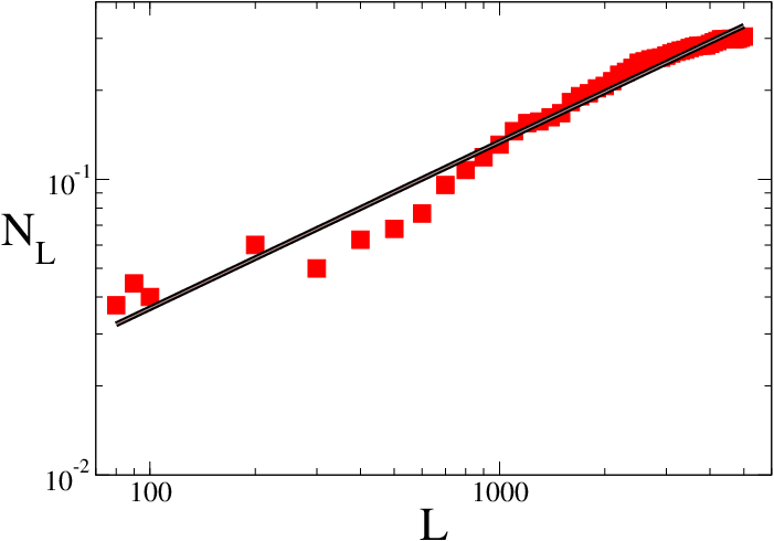
Also the two layers of the BIOGRID network, respectively representing physical (Phys) and genetic (Gen) interactions among proteins, have radically different structures. First of all, the two layers have a different number of non-isolated nodes and a different distribution of the sizes of connected components, with Phys having $N=51697$ non-isolated nodes, while Gen only $N=12590$. Of these nodes, only $9738$ are non-isolated on both layers, meaning that more than $80\%$ of the nodes are active in just one of the two layers, and not in the other. Despite having a smaller number of non-isolated nodes, the Gen layer is much denser than Phys, with an average degree $\langle k^{[Gen]}\rangle\simeq 32$ compared to $\langle k^{[Phys]}\rangle\simeq 11$. Also in this case there is no correspondence between the hubs at the two layers, as shown by the plot in Fig. 2 which reports the fraction $N_{L}$ of those nodes which are found in the top-L ranking of both layers according to the degree. Notice that $N_{L}$ is much smaller than $10\%$ for a wide range of values of $L$ (i.e., up to $L\simeq 600$), meaning that if a node is a hub on one layer there is a quite small probability that it will also be a hub on the other layer. This result is due to the fundamental difference between physical interactions, which produce new protein compounds, with respect to genetic interactions, which trigger the production of other proteins.

Summing up, if we take into account the multi-layered nature of the C.elegans neuronal network and of the BIOGRID protein interaction network we discover new structural patterns, and in particular a poor correspondence of the roles of a node across layers, with a large fraction of the nodes being isolated at least in one of the two layers. These results suggest that representing a system as a multiplex network allows to retain important information, since multi-layer real-world systems are often characterized by non-trivial patterns of node involvement across layers. In the rest of the paper we propose some metrics to quantify these patterns, and we introduce a few models to reproduce and to assess their significance.

Figure 2: (Color online) The fraction $N_{L}$ of nodes which appear in the top $L$ positions according to degree in both layers (Phys and Gen) of the BIOGRID network (squares) scales approximately as a power law $N_{L}\sim L^{0.56}$ (solid line, $r^{2}=0.96$). In particular, less than $20$ nodes appear in both rankings up to $L\simeq 300$, meaning that there is almost no correlation between the degrees of the a node at the two layers, and that it is very unlikely that a node is a hub on both Gen and Phys.

Figure 3: (color online) Distributions of node-activity for (a) the six multiplex networks of continental airlines and for (b) APS and IMDb. In all airline networks $P(B_{i})$ can be fitted by power-laws with exponents ranging from $1.8$ to $2.3$ (the exponents, together with the corresponding p-values in parenthesis, are reported in the legend). This means that the typical number of layers in which a node is active is subject to unbounded fluctuations. The plots in panel (a) have been vertically displaced to enhance readability.

III Correlations of node activity

Let us consider a multiplex network with $N$ nodes and $M$ layers. Such a network can be naturally described by giving a set of $M$ adjacency matrices, one for each layer, $\{A^{[1]},A^{[2]},\ldots,A^{[M]}\}\in\mathbb{R}^{N\times N\times M}$, so that the element $a^{[\alpha]}_{ij}=1$ if node $i$ and $j$ are connected at layer $\alpha$, while $a^{[\alpha]}_{ij}=0$ otherwise. Notice that in this particular kind of multiplex networks, a node $i$ effectively consists of $M$ replicas, one for each layer, and inter-layer connections among these replicas have no explicit cost associated Battiston2014 . These multiplexes are sometimes referred in the literature as colored-edge networks Kivela2014 . In this framework, the properties of the nodes are represented by vectorial variables. For instance, we can associate to each node $i$ of the multiplex a multi-degree, i.e. a $M$-dimensional vector

$$\bm{k}_{i}=\left\{k^{[1]}_{i},k^{[2]}_{i},\ldots,k^{[M]}_{i}\right\}$$ (1)

such that $k^{[\alpha]}_{i}$ denotes the degree of $i$ at layer $\alpha$. A node can in fact participate with a different number of edges to each layer, and can also be isolated in some of the layers. Intuitively, the presence and number of edges incident in a node is a first indication of the activity or importance of that node at that layer. But there is another level of complexity, typical of multiplex structures, which is related to the importance or role of one layer with respect to another in terms of the fraction of connected nodes and of the relative number of edges of a certain kind. For example, in the APS multiplex the number of active nodes in the two Condensed Matter layers (layer 6 and layer 7) account for more than one third of the total number of active nodes at all layers, while the number of edges connecting authors working in General Physics, Particle Physics, Nuclear Physics and Astronomy account for more than 99% of all the edges in the multiplex (see Table A-V for details). The additional complexity added by the presence of multiple layers allows for the exploration of several kinds of structural properties. In particular, we are interested here in detecting, quantifying and modeling the existence of correlations of node activity across layers (vertical analysis) and of correlations among layer structures (horizontal analysis). To this aim, we define in the following some basic quantities which characterize, respectively, the activity of nodes and layers.

III.1 Node activity

We say that node $i$, with $i=1,2,\ldots,N$, is active at layer $\alpha$ if $k^{[\alpha]}_{i}>0$. We can then associate to each node $i$ a node-activity vector

$$\bm{b}_{i}=\left\{b^{[1]}_{i},b^{[2]}_{i},\ldots,b^{[M]}_{i}\right\}$$ (2)

where

$$b^{[\alpha]}_{i}=1-\delta_{0,k^{[\alpha]}_{i}}$$

i.e., $b^{[\alpha]}_{i}=1$ if node $i$ has at least one edge at layer $\alpha$, and is 0 otherwise. We call node-activity $B_{i}$ of node $i$ the number of layers on which node $i$ is active:

$$B_{i}=\sum_{\alpha}b^{[\alpha]}_{i}$$ (3)

By definition we have $0\leq B_{i}\leq M$. Notice that the node-activity vector $\bm{b}_{i}$ provides a compact, yet incomplete (because it does not take into account the number of links) representation of the involvement of node $i$ at the different layers of the multiplex. However, we will show that it contains useful information.

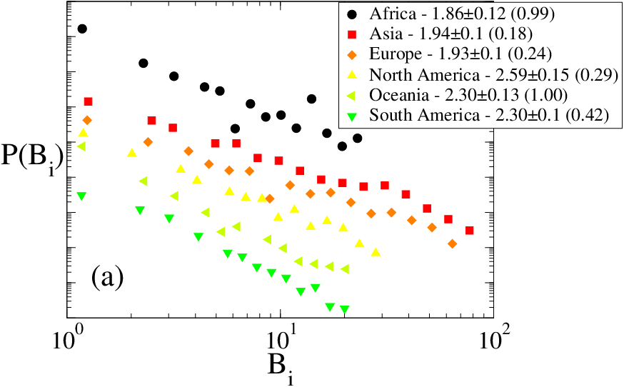
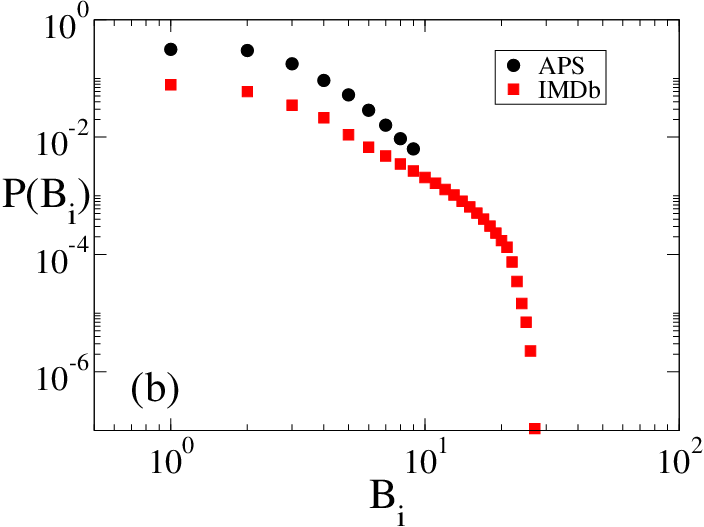
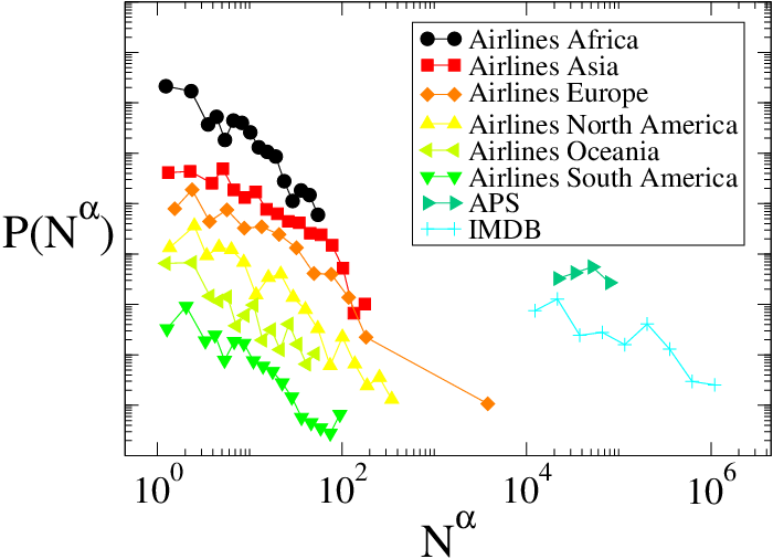
Distribution of node-activity. — In Fig. 3 we report the distributions of node-activity obtained for the multiplex networks constructed from OpenFlight, APS and IMDb. Interestingly, in the airport networks the distributions are well fitted by a power-law function $P(B_{i})\sim B_{i}^{-\delta}$, with exponents $\delta$ in the range $[1.8,2.4]$. The values of the exponents were obtained through the maximum-likelihood estimator Clauset2007 . The most heterogenous distribution is that of the African airplane multiplex network ($\delta\simeq 1.86$), reported as black circles in Fig. 3(a), while the two most homogeneous distributions are those of the airline networks of South America and Oceania (both characterised by $\delta\simeq 2.3$). The power-law behaviour of node-activity indicates that there is no meaningful typical number of layers on which a node is active, since for $\delta<3.0$ the fluctuations on this number are unbound as $M$ grows. A scale-free distribution of node-activity in the airport multiplex networks indicates that the majority of airports usually tend to be connected only by a relatively small number of airlines (between $68\%$ and $89\%$ of all the airports in each multiplex are active in less than $5$ layers), but some “outliers” exist which are connected by a relatively large number of different airlines (at least one airport in each multiplex is active in $10\%$ to $30\%$ of the layers). Similar considerations can be made for APS and IMDb, where the vast majority of authors and actors are active in just one or a few layers, while a few outliers are found active in almost all layers.

In the same spirit of what is done in single-layer networks, where nodes having a relatively high number of connections in a network are called hubs, we call multi-active hubs those outlier nodes of a multiplex which are active in a large fraction of layers. However, as we will better see in Section V, in real-world systems node-activity is not strictly correlated to the total number of edges incident in a node, so that a node might be a multi-active hub without being a hub in the classical sense (of having many links) in any of the layers. In particular, there exist nodes having, at the same time, a large number of incident edges and a small node-activity (e.g., they might be active in just a few layers, or even in one layer only), and also nodes having a relatively small number of edges which are instead active on almost all layers.

Distribution of node-activity vectors. — The node-activity $B_{i}$ accounts only for the number of layers at which node $i$ is active, discarding any information about which are these layers. As a matter of fact, two nodes $i$ and $j$ might have the same value of node-activity but they can be involved in different layers. So it is interesting to look also at how the node-activity vectors ${\bf b}_{i},i=1,2,\ldots,N$, are distributed, to see the relevant frequency of different node-activity patterns. First of all it is important to notice that the actual number of distinct node-activity vectors observed in a multiplex can in general be much smaller than the total possible number of such vectors, which is equal to $2^{M}-1$ (if we take into account only nodes that are active on at least one layer). For instance, while in the APS multiplex we observe $981$ out of the $1023$ possible node-activity vectors (with an average of $173.6$ nodes having the same vector), in IMDb we observe only around $123000$ out of more than $2.6\times 10^{8}$ possible vectors (with an average of around $17.4$ nodes having the same vector).

In Fig. 4(a) we show the Zipf’s plot of the node-activity vectors for the APS and IMDb multiplex networks. In both cases the distribution of $\bm{b}_{i}$ is a power-law (with a clear exponential cut-off in the case of APS), with an exponent respectively equal to $1.53$ and $1.2$. This means that the majority of the nodes have similar activity patterns, with the highest values of $P({\bf b}_{i})$ always corresponding to nodes active on just one or two layers, while some other node-activity vectors are more rare.

Figure 4: (color online) (a) The Zipf’s plot of the node-activity vectors is a power-law, both for APS and for IMDb. Also the rank distribution $P(\bm{b}_{i}|B_{i})$ restricted to nodes having a given value of node-activity $B_{i}$, for (b) APS and (c) IMDb, are power-laws with exponential cut-off. The esponents of the power-laws range between $0.5$ (dot-dashed blue line) and $1.0$ (dashed black line).

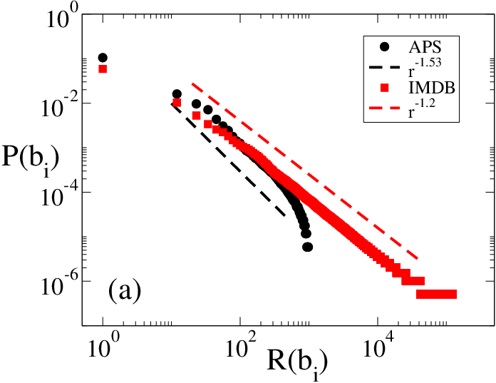
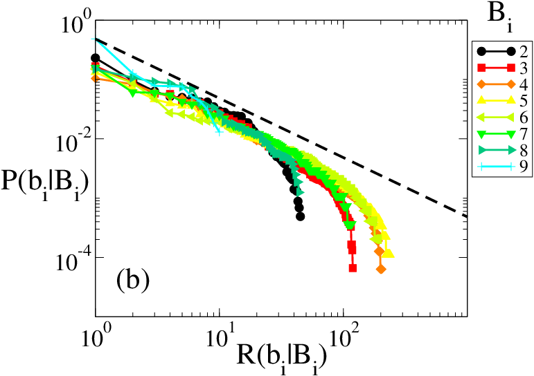
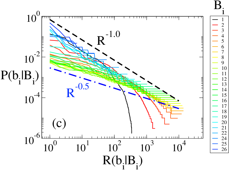
This result is also confirmed by Fig. 4(b) and 4(c) where we report, respectively for APS and IMDb, the rank distributions, i.e., the Zipf’s plots of the probability $P(\bm{b}_{i}|B_{i})$ of node-activity vectors $\bm{b}_{i}$ restricted to nodes active on exactly $B_{i}$ layers, as a function of the rank $R(\bm{b}_{i}|B_{i})$.

The various curves correspond to different values of $B_{i}$. Notice that in general $P(\bm{b}_{i}|B_{i})$ is heterogeneous and is a power-law for the large majority of values of $B_{i}$. This means that a large fraction of the nodes having the same value of node-activity share also the same activity pattern across layers, while some outlier nodes have quite peculiar activity patterns. In the case of IMDb, for instance, of all the actors who have worked on exactly two genres, around $20\%$ are specialised in Short and Drama (layers 23 and 9) or Short and Comedy (layer 23 and 6), while only one actor has acted both on Fantasy and War movies (respectively layer 11 and 27) and only two have acted both in an Adult movie and in a Family movie.

Figure 5: (color online) Distribution of layer-activity for the continental airline networks, APS and IMDb. In the six multiplex of continental airlines, which consist of $O(10^{2})$ layers, $P(N^{\alpha})$ has a clear power-law shape. A somehow heterogeneous behaviour is also observed for IMDb, although the number of layers is not large enough to allow a meaningful fit. The plots were vertically displaced to enhance readability.

III.2 Layer activity

The activity of a given layer $\alpha$, with $\alpha=1,2,\ldots,M$, depends on the patterns of node activities at that layer, and can be represented by the layer-activity vector:

$${\bf d}^{[\alpha]}=\left\{b^{[\alpha]}_{1},b^{[\alpha]}_{2},\ldots,b^{[\alpha]}_{N}\right\}.$$ (4)

We define the layer-activity of layer $\alpha$ as the number $N^{[\alpha]}$ of active nodes in $\alpha$, which is equal to the number of non-zero elements of ${\bf d}^{[\alpha]}$:

$$N^{[\alpha]}=\sum_{i}b^{[\alpha]}_{i}$$ (5)

By definition we have $0\leq N^{[\alpha]}\leq N$.

Distribution of layer-activity. — In Fig. 5 we show the distributions of $N^{[\alpha]}$ for all the multiplex networks with more than two layers. Interestingly, as found for $B_{i}$, also the distribution of $N^{[\alpha]}$ is heterogeneous, and has a marked power-law behavior for the continental airlines networks, which have a larger number of layers. This confirms that, not only the activity of nodes across layers is heterogeneous, but also that not all layers have the same importance in the overall organisation of the system. For instance, a large fraction of all the layers of the continental airlines multiplexes have no more than $N^{[\alpha]}=10$ active nodes. However, some layers contain up to a few hundred active nodes (which account for $10\%$ up to $30\%$ of all the nodes). This means that, on average, the removal of one layer at random from the system, i.e., the removal of all the routes operated by one airline company, will cause only minor disruptions, but in some specific cases such a removal might break the system apart.

Figure 6: (color online) The pairwise multiplexity has a power-law behavior in (a) airline networks, while it is exponential in (b) APS and IMDb. In panel (c) we report a graph of the first 20 airlines in Europe by number of covered airports. Each node of this graph represents a layer of the original multiplex network, while the weight of the edge connecting two nodes is proportional to the fraction of nodes present in both layers. The size of a node is proportional to the number of airports in which the corresponding company operates, while the color (from yellow to red) corresponds to the node strength, which in this case is proportional to the total node overlap with other airlines.

Correlations of layer-activity. — We define here some simple measures to detect and characterize the correlations among layer activities. The first measure we propose is the pairwise multiplexity $Q_{\alpha,\beta}$ of two layers $\alpha$ and $\beta$ defined as:

$$Q_{\alpha,\beta}=\frac{1}{N}\sum_{i}b^{[\alpha]}_{i}b^{[\beta]}_{i}$$ (6)

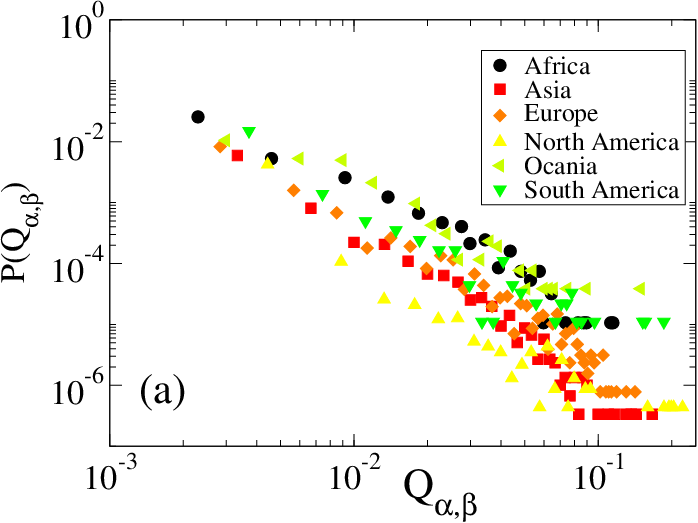
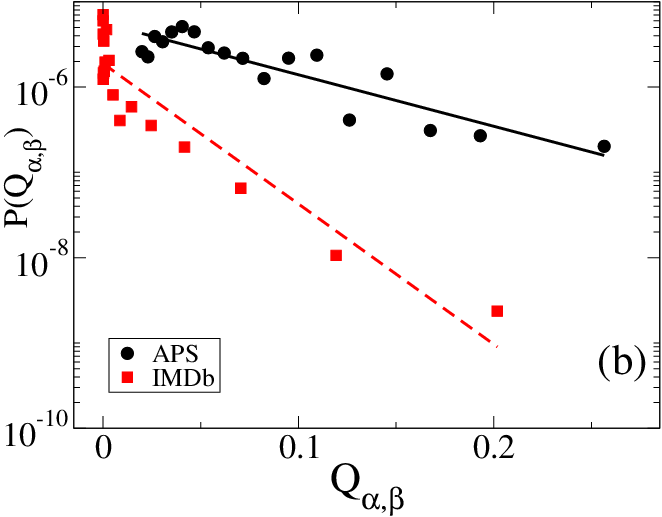
Notice that this quantity is equal to the fraction of nodes of the multiplex which are active on both layers $\alpha$ and $\beta$, and therefore takes values in the range $[0,1]$. The more similar the activity pattern of the nodes at two layers, the higher the multiplexity of two layers is. The distribution of the values of the pairwise multiplexity $P(Q_{\alpha,\beta})$ among all the possible pairs of layers $\alpha$ and $\beta$ is reported in Fig. 6(a)-(b), respectively for the continental airports networks and for APS and IMDb. We first notice that in all the multiplex networks considered only a relatively small fraction of nodes are active at the same time on at least two layers. In particular, in the case of continental airlines the multiplexity has a broad distribution, so that the majority of couples of layers have less than $1\%$ of the nodes in common, while in a few cases the multiplexity can be as high as $20\%$. Also in APS and IMDb the values of pairwise multiplexity are usually below $20\%$, but in this case the distributions exhibit an exponential decay, indicating that there exists a typical scale of pairwise layer multiplexity.

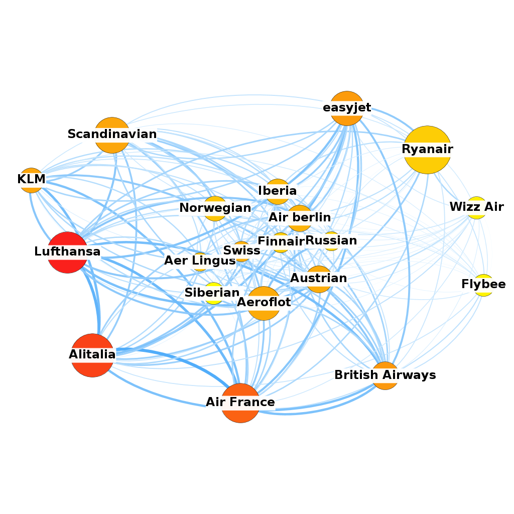
The different behaviour of $P(Q_{\alpha,\beta})$ in the airport networks, with respect to the collaboration networks is probably due to the different meaning of activity at each layer, and also to the different dynamics of node activation in the two cases. In particular, for the airport network, we expect that the competition between airlines operating in the same area produces a small overlap in the activity pattern of the corresponding layers. This is clear shown in Fig. 6(c), where we report the graph representing relationships among the first 20 airlines in Europe operating in the largest number of airports. In this graph each node represents a layer of the original multiplex network, its size is proportional to the corresponding value $N^{[\alpha]}$, the width of an edge is proportional to the pairwise multiplexity of the corresponding layers, i.e. the fraction of nodes active on both layers, and the color of nodes indicates the total multiplexity, i.e. the sum of the values of pairwise multiplexity incident on a node (red is maximum, yellow is minimum). Notice that national companies, like Lufthansa, Alitalia and Air France, tend to have a large overlap with other airlines, i.e. to serve similar sets of airports, while low-cost airlines, like easyJet, Ryanair, Wizz Air and Flybee, systematically tend to avoid overlaps with other companies. The relatively small values of pairwise multiplexity found in these real-world multiplex networks may have an impact on the dynamics of processes occurring over them, such as opinion formation, epidemic spreading, percolation or immunization Radicchi2015 ; Diakonova2015 . Indeed, since only a relatively small fraction of nodes are active on two layers at the same time then the removal of just a few of these nodes might result in a massive disruption of the multiplex network, and can thus slow down dramatically either the spreading of an epidemic or the diffusion of information. This aspect has to be properly taken into account when considering dynamical processes on multiplex networks.

Figure 7: (color online) The distribution of the normalised Hamming distance $H_{\alpha,\beta}$ between all the possible pairs of layers on various multiplex networks. Notice that $P(H)$ increases exponentially for the continental airlines networks.

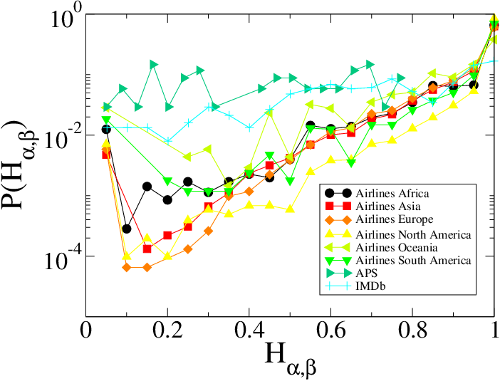
Another measure to quantify the relative overlap between two layers at the level of node activity is the normalised Hamming distance between the two corresponding layer-activity vectors:

$$H_{\alpha,\beta}=\frac{\sum_{i}b^{[\alpha]}_{i}(1-b^{[\beta]}_{i})+(1-b^{[\alpha]}_{i})b^{[\beta]}_{i}}{\min(N^{[\alpha]}+N^{[\beta]},N)}$$ (7)

$H_{\alpha,\beta}$ is equal to the number of differences in the activities of the two layers divided by the maximum possible number of such differences, and takes values in $[0,1]$. In particular, $H_{\alpha,\beta}=0$ if ${\bf d}^{[\alpha]}={\bf d}^{[\beta]}$, while $H_{\alpha,\beta}=1$ when all the active nodes at layer $\alpha$ are not active at layer $\beta$. In Fig. 7 we report the distributions of $H_{\alpha,\beta}$ for the continental airlines, for APS and for IMDb. In all the networks considered the measured values of $H_{\alpha,\beta}$ are distributed throughout the whole $[0,1]$ range. However, in the continental networks the distributions have an increasing exponential behaviour, meaning that the normalised Hamming distance is quite large for the vast majority of layer pairs, in accordance with the observation that airports generally have small node-activity (Fig. 5(a)). Conversely, for APS and IMDb the distributions are more homogeneous. It is interesting to notice that in all the systems around $1\%$ of the layer pairs have a normalised distance smaller than $0.05$, corresponding to large overlaps of node activity.

Figure 8: (color online) Distribution of pairwise multiplexity (a) and Zipf’s plot of node-activity (b) for the European airlines multiplex network (solid black line) and the corresponding synthetic networks obtained by four different models, namely: HM (red circles), MDM (orange squares), MSM (green diamonds) and LGM (blue triangles). Notice that LGM fits well the distribution of pairwise multiplexity, and performs better than HM in reproducing the rank distribution of node-activity. The shape of $P(B_{i})$ in MDM and MSM is identical to that of the original multiplex by construction.

IV Models of node and layer activity

The empirical results of Section III suggest that the patterns of node and layer activity in real-world multiplex networks can be quite heterogeneous. In general, real-world multiplex systems tend to be quite sparse, meaning that the majority of nodes participate to only a small subset of all the layers, and given two layers only a small fraction of their nodes are active on both. It is therefore natural to ask whether similar patterns might naturallly arise from a random distribution of node activity across layers or not. Or, in other words, if there is anything special at all in the power-law distributions of node-activity, node-activity vectors, and layer activity, and if the observed behaviour of multiplexity and normalised Hamming distance among layers can be just the result of the juxtaposition of independent layers. We propose here four different multiplex network models and we compare the correlations in node and layer activity observed in real-world multiplexes with those produced by those models. The first three models are null-models to assess the significance of the heterogeneity of the distributions $P(N^{[\alpha]})$, $P(B_{i})$ and $P(\bm{b}_{i})$. The fourth model is instead a generative model which proposes a possible explanation for the observed distributions of pairwise multiplexity and normalised Hamming distance among layers. A software implementation of the four models is available for download at url .

Hypergeometric model (HM). — In this model we fix the numbers $N^{[\alpha]}$ of active nodes at each layer $\alpha$ to be equal to those observed in the original multiplex network. The $N^{[\alpha]}$ nodes to be actived at each layer $\alpha$ are then randomly sampled with a uniform probability from the $N$ nodes of the graph. In this way, the activity of a node at a given layer is uncorrelated from its activity at another layer and, given two layers $\alpha$ and $\beta$, with $N^{[\alpha]}$ active at the first layer and $N^{[\beta]}$ active at the second layer, the probability $p(m;N,N^{[\alpha]},N^{[\beta]})$ that exactly $m$ nodes, with $m=0,\ldots,\min(N^{[\alpha]},N^{[\beta]})$, are active at both layers follows a hypergeometric distribution:

$$p\left(m;N,N^{[\alpha]},N^{[\beta]}\right)=\frac{\displaystyle\binom{N^{[\alpha]}}{m}\binom{N-N^{[\alpha]}}{N^{[\beta]}-m}}{\displaystyle\binom{N}{N^{[\beta]}}}.$$ (8)

Consequently, the average number of nodes active at both layers is equal to ${N^{[\alpha]}N^{[\beta]}}/{N}$, and the expected pairwise multiplexity of the two layers is:

$$\widetilde{Q}_{\alpha,\beta}=\frac{N^{[\alpha]}N^{[\beta]}}{N^{2}}$$ (9)

Similarly, the expected value of the normalised Hamming distance between two layers $\alpha$ and $\beta$ is equal to:

$$\widetilde{H}_{\alpha,\beta}=\frac{\displaystyle\sum_{m=0}^{N^{[\beta]}}\left(N^{[\alpha]}+N^{[\beta]}-2m\right)\times p\left(m;N,N^{[\alpha]},N^{[\beta]}\right)}{\displaystyle\min(N,N^{[\alpha]}+N^{[\beta]})}$$ (10)

Figure 9: (color online) The rank distribution of node-activity vectors in APS (a) and IMDb (b), compared with those of synthetic multiplex networks genrated using MDM and MSM.

Multi-activity Deterministic Model (MDM). — In this model we costruct networks with the same number of layers $M$ and the same number of active nodes $N$ as in a given real-world multiplex network. We consider a node active if it is active at at least one of the $M$ layers of the original network. Then, we associate to each active node $i$ a node-activity vector sampled at random among the $\binom{M}{B_{i}}$ $M$-dimensional binary vectors having exactly $B_{i}$ non-zero entries, where $B_{i}$ is the number of layers in which node $i$ is active in the original network. We name the model Multi-activity Deterministic Model, since the distribution of $B_{i}$ of the original multiplex is preserved, although the correlations in layer activity and the distribution of node-activity vectors are destroyed. The uniform assignment of node-activity vectors also implies that all the layers will have, on average, the same number of active nodes, since the probability that a given node $i$ is active on a given layer $\alpha$ is equal to $B_{i}/M$ and does not depend on $\alpha$. In particular, the expected number of active nodes at layer $\alpha$ is:

$$\widetilde{N}^{[\alpha]}=\frac{1}{M}{\sum_{i}B_{i}},\quad\forall\alpha.$$ (11)

Multi-activity Stochastic Model (MSM). — In this model, we activate node $i$ at layer $\alpha$ with probability $\overline{B_{i}}=B_{i}/M$, where $B_{i}$ is the node-activity of $i$ in the original network. Also in this case the expected activity of each layer is equal to $M^{-1}\sum_{i}B_{i}$, but the node-activity of each node $i$ is a binomially distributed random variable centered around $B_{i}$, so that, differently from MDM, the node-activity distribution is not preserved.

Layer Growth with Preferential Activation Model (LGM). — This model takes into account the fact that real-world multiplex networks exhibit fat-tailed distributions of layer activity, and aims at explaining the power-law distribution of node-activity reported in Fig. 3. The main assumption of the model which is certainly valid for some networks such as the continental airlines, is that a multiplex network grows through the addition of entire layers, each arriving with a certain number of nodes to be activated. Then, each node $i$ of a newly arrived layer is activated (at that layer) with a probability that increases linearly with the number of other layers in which $i$ is already active. From an operational point of view, we start from a multiplex consisting of $N$ nodes (either active or inactive) and $M_{0}$ layers, and we add a layer at each time step. Therefore, at time $t$ the multiplex has $M_{0}+t$ layers. We assume that in the newly arrived layer $\alpha$ there are $N^{[\alpha]}$ nodes to be activated, where $N^{[\alpha]}$ is set equal to the number of active nodes at layer $\alpha$ observed in the original multiplex. Then, we consider all the nodes and activate each node $i$ with probability:

$$P_{i}(t)\propto A+B_{i}(t)$$ (12)

where $A>0$ is a tunable real-valued parameter and $B_{i}(t)$ is the number of layers (among the $M_{0}+t$ existing ones) in which node $i$ is already active. The parameter $A$ is an intrinsic attractiveness which guarantees that also nodes not yet active in the existing layers have a non-zero probability of being activated at a new layer.

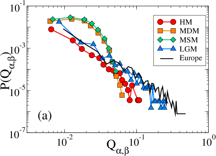
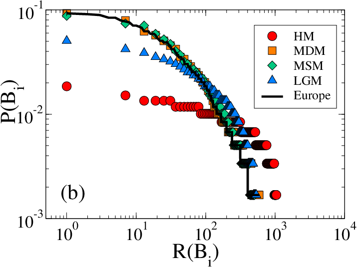
In Figures  8 and  9 we compare the results of the models with some measured quantities in real-world multiplex networks. In particular in Fig. 8(a) we show the distribution of pairwise multiplexity for the European continental airlines and those obtained with the four synthetic models. Remarkably, the distribution of multiplexity of the real system is pretty different from those obtained through HM, MDM and MSM. In particular, both MDM and MSM produce multiplex networks with an exponential-like distribution of multiplexity, while in the original system $Q_{\alpha,\beta}$ is a power-law. HM can somehow reproduce the heterogeneity of $P(Q_{\alpha,\beta})$, even if the typical values of $Q_{\alpha,\beta}$ are much smaller than those observed in the European airline network. The best approximation is obtained through the LGM, which reproduces quite accurately both the shape and the slope of $P(Q_{\alpha,\beta})$. Similarly, in Fig. 8(b) we show the distribution $P(B_{i})$ of node-activity for the original European airlines multiplex and the corresponding synthetic networks. Taking aside MDM and MSM, for which the distribution of node-activity is equal to that of the original network by construction, also in this case LGM is the model which better approximates $P(B_{i})$.

Figure 10: (color online) Density plots of overlapping degree, participation coefficient and node-activity, for APS (top panels) and IMDb (bottom panels). On average, node-activity is positively correlated with both overlapping degree and participation coefficient (the solid line shows the average $\langle B_{i}\rangle$ computed over all the nodes having a certain value of $o_{i}$). However, the fluctuations in the values of $B_{i}$ are quite large in all the cases.

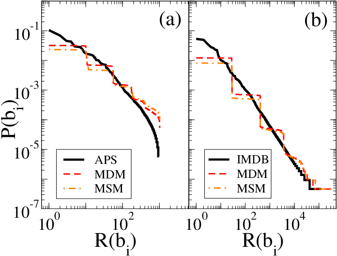
Finally, in Fig. 9 we compare the rank distribution of node-activity vectors in APS and IMDb with those obtained through MDM and MSM (we did not consider LGM since these multiplex have a relatively small number of layers). We notice that the Zipf’s plots of the distributions produced by both MDM and MSM are step-wise constant functions, in which each step corresponds to node-activity vectors having the same value of non-null entries (i.e., of node-activity $B_{i}$). This is due to the fact that in MDM and MSM the probability for a certain node-activity vector to be produced depends only on the corresponding node-activity value $B_{i}$.

The results shown in Fig. 9 suggest that the pattern of node activity across layers in real-world multiplex networks can be quite heterogeneous, and that indeed the activity of a node at a certain layer is often highly correlated with its activity (and inactivity) at other layers. This means that by studying the properties of each layer separately, or, even worse, by aggregating all layers in a single graph, one obtains only a partial picture of the system, while a comprehensive understanding of a multi-layer system requires to take into account the different layers altogether.

V Correlation between activity and degree

In this section we investigate the existence of correlations between the activity of a node and its multidegree, i.e. the number of edges incident in the node at each layer. To a first approximation, the information contained in the multidegree of a node is well described by only two quantities, the overlapping degree and the partecipation coefficient of a node Battiston2014 . Following the definition given in Battiston2014 , we denote the overlapping degree of node $i$ as:

$$o_{i}=\sum_{\alpha}k^{[\alpha]}_{i}$$ (13)

that is the total number of edges incident on $i$. Notice that $o_{i}$ is sometimes called the total degree of node $i$. As the degree is a proxy for the importance of a node in a single-layer network, the overlapping degree of $i$ is a proxy for the overall involvement of node $i$ in the multiplex network. However, the overlapping degree measures only an aspect of the role played by a node in a multiplex system. In fact, if we consider two nodes $i$ and $j$, so that $i$ is active in all the $M$ layers and has $m$ links on each of them, while $j$ is active only on one layer with $m\times M$ links, then we will have $o_{i}=o_{j}=m\times M$. Nevertheless, $i$ and $j$ have quite different roles in the multiplex, since the removal of node $j$ from the system will directly affect the structure of just one layer (namely, the only layer in which $j$ is active), while the removal of $i$ will potentially cause disruptions at all layers. In order to quantify the heterogeneity of the distribution of the links of a node across the layers, one can make use of the multiplex participation coefficient Battiston2014 :

$$P_{i}=\frac{M}{M-1}\left[1-\sum_{\alpha=1}^{M}\biggl{(}\frac{k_{i}^{[\alpha]}}{o_{i}}\biggr{)}^{2}\right].$$ (14)

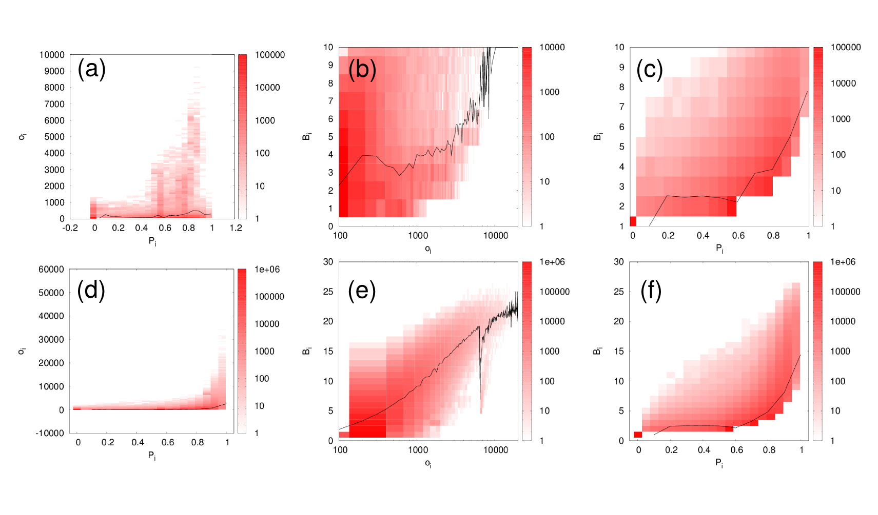
which takes values in $[0,1]$, is equal to $0$ if node $i$ is active in exactly one layer, and tends to $1$ only if the edges of $i$ are equally distributed across all the layers. It has been shown in Refs. Battiston2014 ; Nicosia2014 that important information on the node properties of a multiplex can be obtained by a scatter plot or a density plot of the participation coefficient as a function of overlapping degree. Such diagram have been called multiplex cartography diagrams. In Fig. 10 panels (a) and (d) we plot the multiplex cartography diagrams for APS and IMDb. According to the values of the participation coefficient, nodes can be divided into focused ($P_{i}<1/3$), mixed ($1/3<P_{i}<2/3$) and truly multiplex ($2/3<P_{i}\leq 1$). It is worth noticing that this classification of nodes according to the value of their participation coefficient is in line with the definition of network cartography originally proposed in Ref. Guimera2005 to characterise the role played by single nodes in the organisation in communities, and was adapted to multiplex networks in Ref. Battiston2014 . More principled ways to define the boundaries of the three regions might be based, for instance, on the selection of percentiles of the distribution of participation coefficients, e.g., by setting the boundary between focused and mixed at the $50$-th percentile and the boundary between mixed and multiplex at the $95$-th or $99$-th percentile. However, such a choice would make difficult the comparison of multiplex cartography diagrams associated to distinct multiplex networks.

Nodes with relatively high values of $o_{i}$ are considered hubs. By construction, we do not expect a correlation between $o_{i}$ and $P_{i}$, since the two quantities identify two different aspects of node connectivity. And in fact, the diagrams shown in Fig. 10 exhibit a large variety of patterns. For instance, APS is characterised by a relatively large fraction of mixed hubs (nodes with high $o_{i}$ and intermediate values of $P_{i}$), while almost all the hubs in the IMDb data set are truly multiplex (high values of $P_{i}$).

In a similar way, we can quantify the existence of correlations between the node-activity $B_{i}$ of a node $i$ and the corresponding values of overlapping degree $o_{i}$ and participation coefficient $P_{i}$. In Fig. 10 panel (b) and (e) we report the density plots of node-activity and overlapping degree, respectively for APS and IMDb. As expected, we observe positive correlations between the two quantities $B_{i}$ and $o_{i}$, so that nodes with many links tend to be active on more layers. This is reasonable because a node with a small number of edges cannot be active on a large number of layers. However, the fluctuations around the average value of node-activity for a certain value of overlapping degree (marked by the black solid line in the plots) are quite large.

Figure 11: (color online) Different degree correlation coefficients, namely (a) Pearson’s $r$, (b) Spearman’s $\rho$ and (c) Kendall’s $\tau$ for different couples of layers, and the corresponding distributions (d) are reported for the APS, and show that inter-layer correlations in this system tend to be assortative. A similar pattern is observed in IMDb (panels (e)-(h)). However, some movie genres, like Adult and Talk-Show (respectively corresponding to layer number 2 and number 25 in the diagram) have marked negative inter-layer correlations with almost all the other layers.

Similar relationships exist between node-activity and participation coefficient as shown in Fig. 10(c) and Fig. 10(f), despite the existence of large fluctuations. Namely, nodes having a higher value of participation coefficient usually are active on more layers than nodes having small values of $P_{i}$. This is indeed not surprising, sincethe edges of a node with a higher value of participation coefficient are more uniformly distributed across layers, hence the node will be active on more layers.

VI Inter-layer degree correlations

It has been extensively shown in the literature that single-layer networks are characterised by the presence of degree-degree correlations, meaning that nodes having a certain degree are preferentially connected to other nodes having similar (assortative correlations) or dissimilar degree (disassortative correlations). Social and communication networks are the most remarkable examples of assortative networks, while the vast majority of technological and biological networks exhibit disassortative degree correlations. In addition to the classical intra-layer degree-degree correlations, in a multiplex network we can also define the concept of inter-layer degree-degree correlations.

VI.1 Inter-layer correlation coefficients

A compact way to quantify the presence of inter-layer degree correlations is to make use of one of the standard correlation coefficients to measure how the degree sequences of two layers are correlated. One possibility is the Pearson’s linear correlation coefficient Parshani2010 ; Lee2012 ; Min2013_coop ; Nicosia2014 . If we denote as $k_{i}^{[\alpha]}$ and $k_{i}^{[\beta]}$ the degrees of node $i$ respectively at layer $\alpha$ and layer $\beta$, the Pearson’s correlation coefficient of the two degree sequences is defined as:

$$r_{\alpha,\beta}=\frac{\langle k_{i}^{[\alpha]}k_{i}^{[\beta]}\rangle-\langle k_{i}^{[\alpha]}\rangle\langle k_{i}^{[\beta]}\rangle}{\sigma_{k^{[\alpha]}}\sigma_{k^{[\beta]}}}$$ (15)

To avoid the bias due to the relatively small multiplexity of real-world systems, the averages are taken over all the nodes which are active on both layers. Another possibility is to use the Spearman’s rank correlation coefficient $\rho$ Nicosia2014 :

$$\rho_{\alpha,\beta}=\frac{\sum_{i}\left(R^{[\alpha]}_{i}-\overline{R^{[\alpha]}}\right)\left(R^{[\beta]}_{i}-\overline{R^{[\beta]}}\right)}{\sqrt{\sum_{i}\left(R^{[\alpha]}_{i}-\overline{R^{[\alpha]}}\right)^{2}\sum_{j}\left(R^{[\beta]}_{j}-\overline{R^{[\beta]}}\right)^{2}}}$$ (16)

where $R^{[\alpha]}_{i}$ is the rank of node $i$ due to its degree on layer $\alpha$, and $\overline{R^{[\alpha]}}$ and $\overline{R^{[\beta]}}$ are the average ranks of nodes respectively at layer $\alpha$ and layer $\beta$. Also in this case, only nodes active on both layers are considered in the computation of $\rho_{\alpha,\beta}$. A third option is to use the Kendall’s $\tau$ rank correlation coefficient Nicosia2014 :

$$\tau_{\alpha,\beta}=\frac{n_{c}^{\alpha,\beta}-n_{d}^{\alpha,\beta}}{\sqrt{(n_{0}-n_{\alpha})(n_{0}-n_{\beta})}}.$$ (17)

where $n_{0}=1/2\times NQ_{\alpha,\beta}(NQ_{\alpha,\beta}-1)$ , and $n_{c}^{\alpha,\beta}$ and $n_{d}^{\alpha,\beta}$ are, respectively, the number of concordant pairs and the number of discordant pairs in the two rankings. We say that the two nodes $i$ and $j$ are a concordant pair if the ranks of the two nodes at the two layers agree, i.e. if both $R^{[\alpha]}_{i}>R^{[\alpha]}_{j}$ and $R^{[\beta]}_{i}>R^{[\beta]}_{j}$, or both $R^{[\alpha]}_{i}<R^{[\alpha]}_{j}$ and $R^{[\beta]}_{i}<R^{[\beta]}_{j}$. If a pair of nodes is not concordant, then it is said discordant. Finally, $n_{\alpha}$ and $n_{\beta}$ account for the number of rank ties in the two layers.

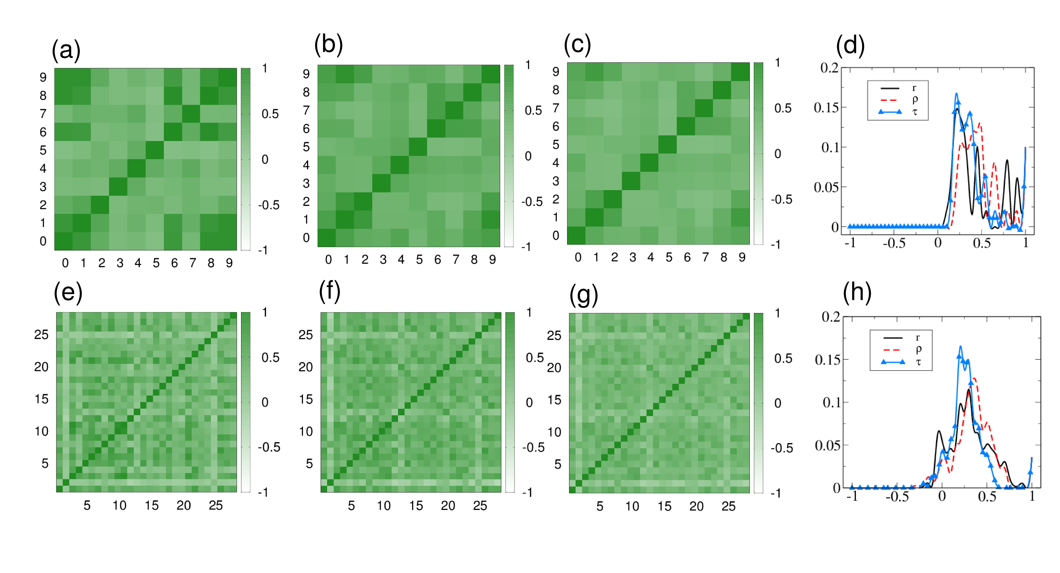
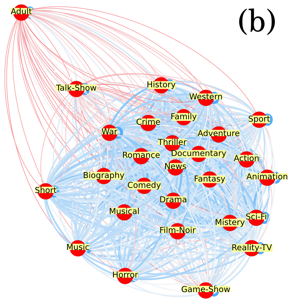
We have computed the three above pairwise correlation coefficients for the APS and for the IMDb multiplex networks. The results are shown in Fig. 11. We notice that each of the three coefficients show a slightly different behaviour. Nevertheless, it is clear from the Figure that inter-layer correlations in APS are exclusively assortative, while in IMDb we can observe both positive and negative correlations. In particular, the degree of nodes at layer 2 (Adult movies) and at layer 25 (Talk-Shows) are negatively correlated with the degree on all the other layers, whilst being positively correlated to each other. These results indicate that it is pretty uncommon —even if not impossible— for an actor of Adult movies, to take part in a Family movie or in a Thriller. In addition to this, the large majority of actors usually prefer to avoid talk-shows, the main exception being porn stars. The presence of negative inter-layer degree correlations in the IMDb multiplex network is highlighted in the distributions of the three correlation coefficients reported in panel (h). It is interesting that, in most of the cases, also the inter-layer degree correlations in multiplex social networks are assortative. This is in agreement with the common belief that intra-layer degree-degree correlations in single-layer social systems are always of the assortative type. However, cases such as the IMDb are an example that disassortativity is possible in social networks when they are not aggregated, and treated as multiplex networks.

It is important to stress that, although the Spearman’s and Kendall’s rank correlation coefficients are able to capture, at least to some extent, the presence of non-linear correlations in the rankings induced by two degree distributions, the choice of which coefficient is more appropriate to quantify inter-layer correlations might in general depend on the actual system under study. As we will see in the following, a more accurate way of measuring such correlations is by means of inter-layer degree correlation functions.

VI.2 Inter-layer correlation functions

The complete information on degree correlations in single-layer networks is contained in the joint degree distribution function $P(k,k^{\prime})$ or, equivalently, in the conditional degree distribution $P(k^{\prime}|k)$, which respectively denote the probability that a randomly chosen link connects a node of degree $k$ to a node of degree $k^{\prime}$, and the probability that a link from a node of degree $k$ connects a node of degree $k^{\prime}$. A convenient quantity that is commonly used to detect degree correlations is the degree correlation function, defined as the average degree of the first neighbours of a node having a certain degree $k$:

$$k_{nn}(k)=\overline{k^{\prime}}(k)=\sum_{k^{\prime}}k^{\prime}P(k^{\prime}|k)$$

In fact, in single-layer networks with assortative degree correlations $k_{nn}(k)$ will be an increasing function of $k$, while in disassortative networks $k_{nn}(k)$ will decrease with $k$. An interesting result is that in many cases of real-world complex networks we have $k_{nn}(k)\sim k^{\nu}$, so that the correlation exponent $\nu$ can be used to quantify the sign and intensity of degree-degree correlations Vespignani2001 ; Pastor-Satorras2001 .

Figure 12: (color online) The Zipf’s plot of the distribution of multi-degree in (a) APS and (b) IMDb have a power-law tail with exponent close to $1.0$. However, the multi-degree distribution might be affected by large fluctuations. In fact, in both cases around $90\%$ of the multi-degree vectors are present only once, and more than $95\%$ are observed less than four times.

Figure 13: (color online) The inter-layer pairwise degree correlation function $\overline{k^{[\beta]}}(k^{[\alpha]})$ is shown for (a) C.elegans and BIOGRID and for various couples of layers $\alpha$ and $\beta$, respectively, in (b) APS and (c) IMDb. The lines reported are fit obtained by a power law of the form $\overline{k^{[\beta]}}(k^{[\alpha]})\sim({k^{[\alpha]}})^{\mu}$. The plots are vertically displaced to enhance readability.

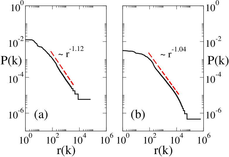
In a multiplex network the complete information about inter-layer correlations is contained in the joint probability $P(k^{[1]},\ldots,k^{[M]})$, which represents the probability that a randomly chosen node has degree $k^{[1]}$ at layer 1, degree $k^{[2]}$ at layer 2, and so on, and is nothing else than the multi-degree distribution of the system $P(\bm{k})$. As an example, we report in Fig.12 the Zipf’s plot of the distribution of multi-degree for APS and IMDb. Interestingly, both distributions exhibit a power-law behavior with a negative exponent around $-1.0$. The inter-layer correlations between layers $\alpha$ and $\beta$ can be studied by constructing the pairwise joint and conditional probability distributions

$$P(k^{[\alpha]},k^{[\beta]})\quad\text{and}\quad P(k^{[\beta]}|k^{[\alpha]})$$

The first quantity denotes the probability that a randomly chosen node has degree $k^{[\alpha]}$ at layer $\alpha$ and degree $k^{[\beta]}$ at layer $\beta$, while the latter denotes the probability that a node having a given degree $k^{[\alpha]}$ at layer $\alpha$ has degree $k^{[\beta]}$ at layer $\beta$. In the same spirit of the degree correlation function defined for single-layer networks, given two layers $\alpha$ and $\beta$ we can define the two inter-layer degree correlation functions:

$$\overline{k^{[\beta]}}(k^{[\alpha]})=\sum_{k^{[\beta]}}k^{[\beta]}P(k^{[\beta]}|k^{[\alpha]})$$ (18)

and

$$\overline{k^{[\alpha]}}(k^{[\beta]})=\sum_{k^{[\alpha]}}k^{[\alpha]}P(k^{[\alpha]}|k^{[\beta]}).$$ (19)

These two quantities quantify the average degree at layer $\beta$ (resp. $\alpha$) of a node having a degree equal to $k^{[\alpha]}$ (resp. $k^{[\beta]}$) at layer $\alpha$ (resp. $\beta$). Being average quantities, we expect smaller fluctuations than if we directly plotted the two-dimensional functions $P(k^{[\alpha]},k^{[\beta]})$ and $P(k^{[\beta]}|k^{[\alpha]})$. Again, the idea is that an increase (decrease) of $\overline{k^{[\beta]}}(k^{[\alpha]})$ as a function of $k^{[\alpha]}$ is a sign of the presence of assortative (disassortative) inter-layer degree correlations between $\alpha$ and $\beta$.

Figure 14: (color online) The inter-layer correlation pattern of (a) APS and (b) IMDB is evident by considering a graph whose nodes correspond to layers and the weight of the edges is the value of the inter-layer correlation exponent $\mu$. In the figure blu weights correspond to positive correlations while red weights to negative ones. Panel (c): the distribution of the values of the inter-layer correlation exponent $\mu$ in APS (solid black line) and in IMBd (dashed red line). Notice that while inter-layer degree correlations are always positive in APS, the layers of IMDb might be either positively or negatively correlated.

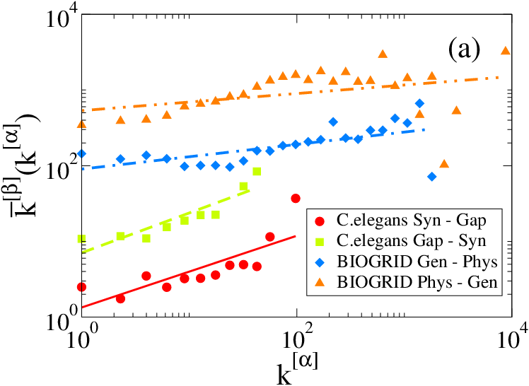
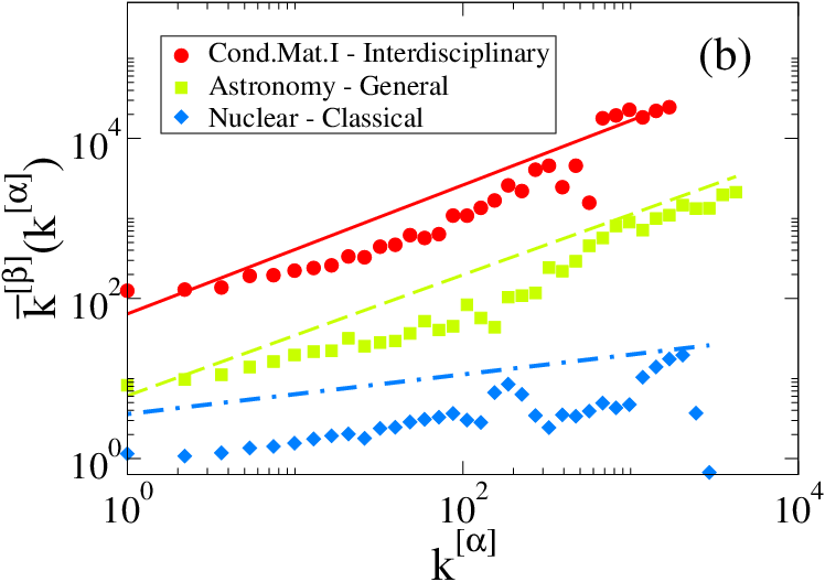
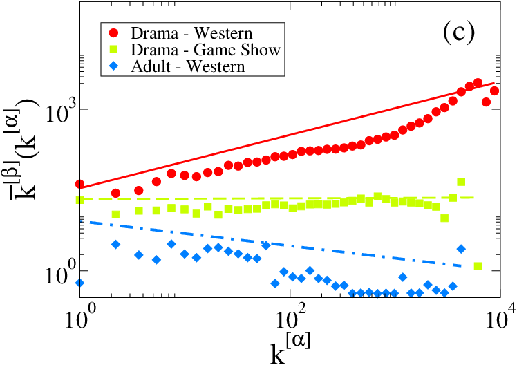
In Fig. 13 we show some typical examples of pairwise inter-layer degree correlation functions in C.elegans, BIOGRID, APS and IMDb. Both in the two biological networks and in APS we observe an increasing behavior of $\overline{k^{[\beta]}}(k^{[\alpha]})$ as a function of $k^{[\alpha]}$, denoting the presence of assortative inter-layer degree correlations. For the multiplex network of movie actor collaborations we find instead pairs of layers with assortative or disassortative inter-layer degree correlations, and also pairs of uncorrelated layers. As an example of positively correlated genres in the IMDb we report the couple Drama-Western. The couple Adult-Western is instead negatively correlated, while Drama Movies are not correlated with Game Show, as witnessed by the fact that $\overline{k^{[\beta]}}(k^{[\alpha]})$ shows no dependence on $k^{[\alpha]}$. It is worth noticing that also inter-layer correlation functions can be well fitted, in most of the cases, by power-laws in the form $\overline{k^{[\beta]}}(k^{[\alpha]})\sim({k^{[\alpha]}})^{\mu}$, so that for each network, and for each ordered pair of layers $(\alpha,\beta)$, it is possible to extract the inter-layer correlation exponent $\mu$. We can therefore say that we observe assortative, neutral or disassortative correlations, depending on the fact that the sign of $\mu$ is respectively positive, null or negative. The absolute value of $\mu$ then give information on the intensity of the correlations. Notice that in general, according to the definition of $\overline{k^{[\alpha]}}(k^{[\beta]})$, the exponent of $\overline{k^{[\beta]}}(k^{[\alpha]})$ might be diffrent from the esponent of $\overline{k^{[\alpha]}}(k^{[\beta]})$, as happens for instance in Fig. 13(a) for the layers of C.elegans and BIOGRID.

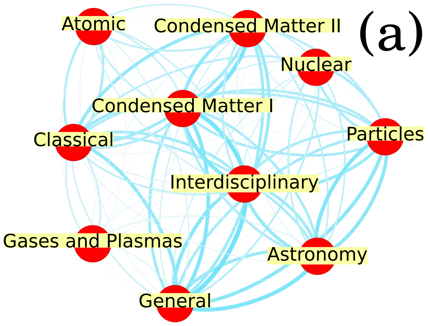
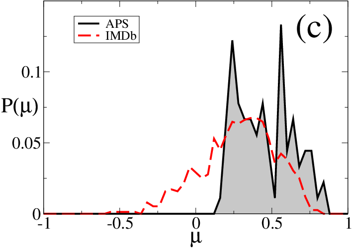
In Fig. 14 we report a graphical representation of the inter-layer degree correlation patterns in APS and in IMDB and we also show the corresponding distribution of inter-layer correlation exponents observed in the two systems. Each node of the graphs shown in Fig. 14(a)-(b) corresponds to a layer of the multiplex, and the color of a link represents the sign and magnitude of the exponent of the inter-layer correlation function between two layers (red for negative exponents and blue for positive ones). It is evident that while in APS inter-layer degree correlations are always positive, in IMDb they might be either positive or negative. Notice also that the only layers in IMDB having negative degree correlations with the others are those corresponding to Adult movies and Talk-Shows.

VII Models of inter-layer degree correlations

We propose here two different models to reproduce the observed patterns of pairwise inter-layer degree correlations. The first model is based on the tuning of the Spearman rank correlation coefficient $\rho_{\alpha,\beta}$, while the second one allows to obtain an inter-layer correlation function $\overline{k^{[\beta]}}(k^{[\alpha]})\sim({k^{[\alpha]}})^{\mu}$. with a prescribed value of the correlation exponent $\mu$. Both models are based on simulated annealing.

VII.1 Model for $\rho$

Let us consider two graphs with the same number of nodes $N$. If we want to construct a two-layer multiplex network using the two graphs respectively as layer $\alpha$ and layer $\beta$ of the multiplex, we need to couple the nodes of the two graphs in such a way that each node of layer $\alpha$ is connected with exactly one node on the other layer $\beta$. Such a coupling can be realized in many different ways, and in particular it can be chosen in order to obtain a given level of inter-layer degree correlation, for instance a given value of the Spearman rank correlation coefficient $\rho_{\alpha,\beta}$. The coupling/correspondence between the nodes of the two graphs can be described by a $N\times N$ matrix $\mathcal{S}=\{s_{ij}\}$ that we call assignment. Entry $s_{ij}=1$ if node $i$ in layer $\alpha$ corresponds to node $j$ in layer $\beta$. Since we have a one-to-one correspondence between the nodes of the two graphs we have to impose $\sum_{j}s_{ij}=1,\>\forall i$. For simplicity in the notation, let us denote by $x_{i}$ the rank of node $i$ in layer $\alpha$, as induced by the degree sequence $\{k^{[\alpha]}_{i}\}$, and by $y_{i}$ the rank of node $i$ in layer $\beta$, as induced by $\{k^{[\beta]}_{i}\}$. In this case the Spearman’s rank correlation coefficient corresponding to the assignment $\mathcal{S}$ can be written as

$$\rho=\frac{\sum_{i,j}s_{ij}(x_{i}-\bar{x})(y_{j}-\bar{y})}{\sqrt{\sum_{i}(x_{i}-\bar{x})^{2}\sum_{j}(y_{j}-\bar{y})^{2}}}$$ (20)

This equation can be also expressed in the form

$$\frac{\sum_{ij}s_{ij}x_{i}y_{j}+C}{D}$$ (21)

where

$$C=N\bar{x}\bar{y}-\bar{y}\sum_{i}x_{i}-\bar{x}\sum_{i}y_{i}$$ (22)

and

$$D=\sqrt{\sum_{i}(x_{i}-\bar{x})^{2}\sum_{j}(y_{j}-\bar{y})^{2}}$$ (23)

are two constants which depends only on the two rankings $\{x_{i}\}$ and $\{y_{i}\}$, and not on the actual assignment $\mathcal{S}$. Therefore, the Spearman’s correlation coefficient is uniquely determined by the term $\sum_{i,j}s_{ij}x_{i}y_{j}$, i.e. by the adjacency matrix $\mathcal{S}$. Consequently, one should in principle be able to obtain any prescribed value ${\rho}^{*}$ of the Spearman rank correlation coefficient by appropriately changing the assignment, i.e. by finding a matrix ${\mathcal{S}}^{*}=\{{s^{*}}_{ij}\}$ so that

$$\frac{\sum_{i,j}{s^{*}}_{ij}x_{i}y_{j}+C}{D}={\rho^{*}}$$ (24)

For a generic assignment $\mathcal{S}$ we have:

$$\frac{\sum_{i,j}s_{ij}x_{i}y_{j}+C}{D}=\rho_{\mathcal{S}}\neq{\rho^{*}}$$

which is associated to the cost function $F(\mathcal{S})=|\rho_{\mathcal{S}}-{\rho^{*}}|$.

Algorithm 1 Simulated annealing for ${\rho^{*}}$

0:  $\{\bm{k}_{i}\}$, $\mathcal{S}=\{s_{ij}\}$, ${\rho^{*}}$, $\varepsilon$

0:  $\mathcal{S^{\prime}}=\{s^{\prime}_{ij}\}$ so that $\rho={\rho^{*}}$

1:  compute $\rho_{\mathcal{S}}$

2:  $F(\mathcal{S})$ $\leftarrow$ $|\rho_{\mathcal{S}}-{\rho^{*}}|$

3:  while $F(\mathcal{S})>\varepsilon$ do

4:     select two inter-layer edges, $(i,j)$ and $(k,\ell)$, at random

5:     replace $(i,j)$ with $(i,\ell)$ and $(k,\ell)$ with $(k,j)$

6:     compute $\rho_{\mathcal{S}^{\prime}}$

7:     $F(\mathcal{S}^{\prime})$ $\leftarrow$ $|\rho_{\mathcal{S}^{\prime}}-{\rho^{*}}|$

8:     if $F(\mathcal{S}^{\prime})<F(\mathcal{S})$ then

9:        $\mathcal{S}$ $\leftarrow$ $\mathcal{S}^{\prime}$

10:     else

11:        swap $F(\mathcal{S})$ and $F(\mathcal{S}^{\prime})$ with probability $p=e^{-(F(\mathcal{S}^{\prime})-F(\mathcal{S}))/\gamma}$

12:     end if

13:     $F(\mathcal{S})$ $\leftarrow$ $|\rho_{\mathcal{S}}-{\rho^{*}}|$

14:  end while

15:  return  $\mathcal{S}$

The basic idea is then to subsequently modify the structure of the assignment in order to minimize $F(\mathcal{S})$. We will make use of a simulated annealing algorithm which works as follows. We start from an initial random assignment $\mathcal{S}$, and we compute its associated cost function $F(\mathcal{S})$. Then, we select two edges $e_{1}=(i,j)$ and $e_{2}=(k,\ell)$ of $\mathcal{S}$, uniformly at random so that $e_{1}\neq e_{2}$, and we consider the adjacency matrix associated to the assignment $\mathcal{S}^{\prime}$ obtained from $\mathcal{S}$ by replacing $e_{1}$ and $e_{2}$ with $e_{1}^{\prime}=(i,\ell)$ and $e_{2}^{\prime}=(k,j)$. We compute $F(\mathcal{S}^{\prime})$, and we accept the new assignment $\mathcal{S}^{\prime}$ with a probability

$$p=\begin{cases}1&\text{ if }F(\mathcal{S}^{\prime})<F(\mathcal{S})\\ e^{-\frac{F(\mathcal{S}^{\prime})-F(\mathcal{S})}{\gamma}}&\text{otherwise}\end{cases}$$ (25)

where $\gamma$ is a parameter. This scheme, whose pseudo-code is reported in Algorithm 1, will favour changes to the adjancency matrix which contribute to minimize the function $F$, but it also allows to explore ergodically all the possible configurations of $\mathcal{S}$, by accepting unfavourable changes with a finite probability. Notice that, due to the discrete nature of the assignment problem and depending on the characteristics of the two rankings under consideration, it might happen that there exists no assignment which produces exactly the desired value ${\rho^{*}}$. Consequently, the algorithm will stop when $F(\mathcal{S})<\varepsilon$, where $\varepsilon$ is a threshold set by the user. Moreover, in order to avoid any bias due to the relatively small multiplexity of real-world systems (i.e., to the relatively small fraction of nodes which are active on both $\alpha$ and $\beta$, for any choice of $\alpha$ and $\beta$), it is usually better to run the algorithm only on the nodes which are active on both the layers considered. In the generic case of $M$-layer multiplex networks one can iterate this algorithm in order to set the values of $\rho_{\alpha,\beta}$ for up to $M-1$ pairs of layers.

As an example, we report in Fig. 15 the values of $\rho_{\alpha,\beta}$ measured for the APS and for the IMDb, together with those obtained in the synthetic multiplex networks constructed by using the proposed algorithm. Each synthetic network was constructued by keeping the distribution of node-activity vectors of the original multiplex, and by reassigning at random the degrees of the active nodes at each layer, sampling them from the same distribution observed in the real multiplex. We considered the $M-1$ pairs of layers having consecutive IDs (e.g., couples of layers $(\alpha,\beta)$ such that $\beta=\alpha+1$, for instance $(0,1)$, $(1,2)$ and so on), and we measured the observed inter-layer rank correlation coefficients $\rho_{\alpha,\beta}$. Then, we iterated Algorithm 1, starting from the first two layers, setting ${\rho^{*}}=\rho_{\alpha,\beta}$ and obtaining an optimal assignment of the nodes in $\alpha$ and $\beta$. Keeping fixed this assignment, we run again Algorithm 1 on the second and the third layer of the multiplex, and we obtained the optimal assignment between their nodes, and so forth. By looking at Fig. 15 it is evident that there is a qualitative correspondence between the distributions of $\rho$ in real and synthetic networks, mostly due to the fact that partial ordering is a transitive relation, but in general the difference between the two might be relatively high (up to $0.4$ in APS and up to $0.5$ in IMDb).

Figure 15: (color online) The values of the Spearman correlation coefficient in the original multiplex (left panels) and in that obtained through Algorithm 1 (middle panels) respectively for APS (top) and IMDb (bottom). In the rightmost panel we show the difference between the original distribution of $\rho$ and that obtained in the synthetic network. In both cases, the overall shape of the distribution of inter-layer correlations in the synthetic multiplex looks very similar to the original one. However, the differences in the obtained value of $\rho$ might be quite high. This is due to the fact that Algorithm 1 allows to set only $M-1$ pairs or correlations, over the total $M(M-1)/2$.

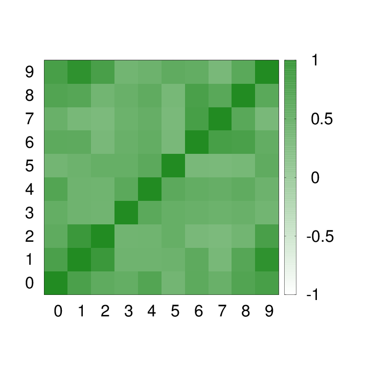
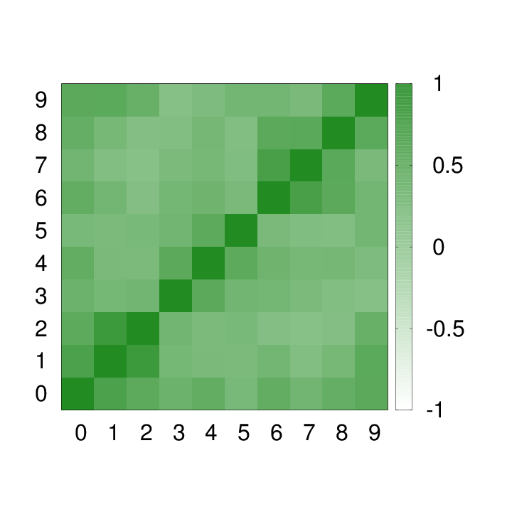
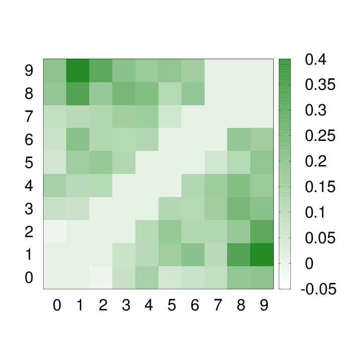
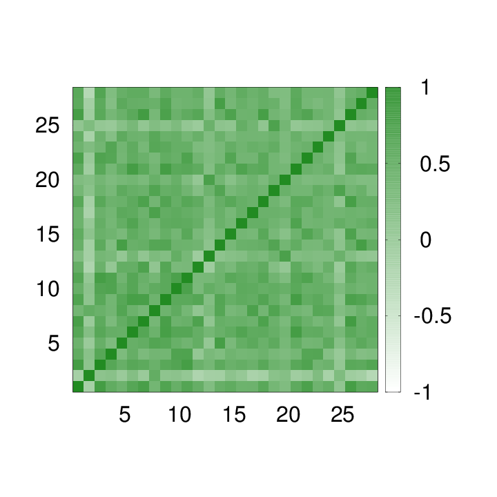
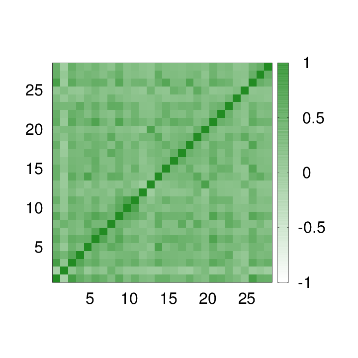
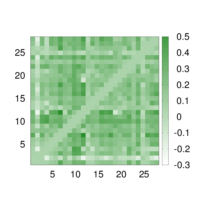
It is important to stress here that Algorithm 1 can be straightforwardly generalized to work with any other node property. In fact the algorithm is based on the comparison of rankings induced by node properties, independently from the fact that these rankings are induced by degree sequences or by any other node attribute. Consequently, the same procedure can be employed to set the magnitude and sign of inter-layer correlations with respect to any real-valued pairs of node properties, such as the clustering coefficient, the betweenness, or the size of the community to which a node belongs. Notice that it would also be possible to consider multi-objective functions which allow to set the correlations for all the $M(M-1)/2$ pairs of layers at the same time. Such variants of Algorithm 1 will be the subject of another work currently in preparation. A software implementation of Algorithm 1 is available for download at url .

Algorithm 2 Simulated annealing for $\bar{q}=ak^{\mu}$

0:  $\{k_{i}\}$, $\{q_{i}\}$, $\{s_{ij}\}$, $\mu$, $\varepsilon$

0:  $\{s^{\prime}_{ij}\}$ so that $|\bar{q}-ak^{\mu}|<\varepsilon$

1:  continue $\leftarrow$ True

2:  while continue is True do

3:     select two nodes, $i$ and $j$, at random

4:     $\Delta_{1}^{\rm old}\leftarrow|\log(q_{i})-\log(a)-\mu\log(k_{i})|$

5:     $\Delta_{2}^{\rm old}\leftarrow|\log(q_{j})-\log(a)-\mu\log(k_{j})|$

6:     $\Delta_{1}^{\rm new}\leftarrow|\log(q_{j})-\log(a)-\mu\log(k_{i})|$

7:     $\Delta_{2}^{\rm new}\leftarrow|\log(q_{i})-\log(a)-\mu\log(k_{j})|$

8:     $F_{\rm old}\leftarrow\Delta_{1}^{\rm old}+\Delta_{2}^{\rm old}$

9:     $F_{\rm new}=\Delta_{1}^{\rm new}+\Delta_{2}^{\rm new}$

10:     if $F_{\rm new}<F_{\rm old}$ then

11:        swap $i$ and $j$ in the second layer and obtain $\{s^{\prime}_{ij}\}$

12:     else

13:        swap $i$ and $j$ with probability $p=e^{-(F_{\rm new}-F_{\rm old})/\gamma}$

14:     end if

15:     compute the best power-law fit $a^{\prime}k^{\mu^{\prime}}$ of $\bar{q}$

16:     if $|\mu-\mu^{\prime}|<\varepsilon$  then

17:        continue $\leftarrow$ False

18:     end if

19:  end while

20:  return  $\{s^{\prime}_{ij}\}$

VII.2 Model for $\overline{k^{[\beta]}}(k^{[\alpha]})$

Analogously to what done in the previous subsection, here we propose an algorithm to tune the assignment of the nodes of two layers $\alpha$ and $\beta$ in order to set a prescribed inter-layer degree correlation function. In particular, we will assume that the desired correlation function is a power-law, i.e. $\overline{k^{[\beta]}}(k^{[\alpha]})=a({k^{[\alpha]}})^{\mu}$, as those observed in real-world multiplex networks. To simplify the notation here we will indicate as $q$ the degree of the node at layer $\beta$ and as $k$ the degree of the node at layer $\alpha$. Then the desired correlation function has the form $\overline{q}(k)=ak^{\mu}$ where the value of $\mu$ is that obtained empirically for a given real network, while $a$ is a constant to be determined. The algorithm is similar to that proposed for the adjustment of the Spearman’s $\rho$ coefficient. We start from a random assignment of nodes $\mathcal{S}$, we select two edges of $\mathcal{S}$ uniformly at random and we try to swap their endpoints in order to locally minimize the difference $\Delta$ between the actual function $\overline{q}(k)$ and the desired one $k^{\mu}$. Favorable swaps, i.e. those which produce smaller values of $\Delta$, are always accepted, while unfavorable ones, i.e. those which produce a local increase in $\Delta$, are accepted with a probability which decays exponentially with the difference in $\Delta$. The main steps of the procedure are summarized in Algorithm 2. There are some technical subtleties to take into account for the implementation of Algorithm 2. First of all, the fact that the coefficient $a$ which multiplies $k^{\mu}$ is in general unknown. Consequently, $a$ is initially set to an arbitrary positive value and then it is adaptively changed as the algorithm proceeds, by setting it equal to the coefficient obtained through the best power-law fit of $\bar{q}(k)$. Updates of $a$ are performed once every $t_{a}$ steps of the algorithm, where $t_{a}$ is a parameter set by the user. A software implementation of Algorithm 2 is available at url .

Figure 16: (color online) The values of the inter-layer degree correlation exponent $\mu$ in the APS multiplex (left) and in a synthetic multiplex network generated through Algorithm 2 (middle). The rightmost panel shows the difference between the exponents observed in the original system and those measured in the synthetic network. Although the left and the middle panel look qualitatively similar, the right panel reveals that the difference in the actual inter-layer degree correlation exponent $\mu$ of the synthetic network might be as high as $0.7$.

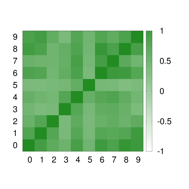
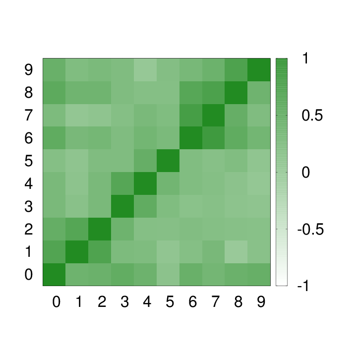
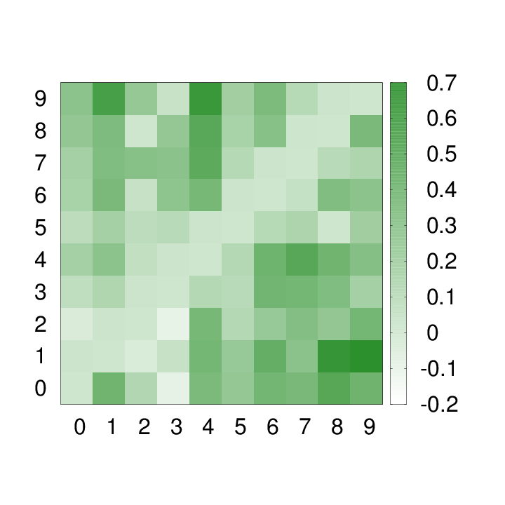
In Fig. 16 we compare the values of the inter-layer degree correlation exponent $\mu$ observed in the APS multiplex and in the synthetic network obtained through Algorithm 2. Despite the distribution of $\mu$ in the synthetic multiplex looks qualitatively similar to that of the original system, the difference in the actual value of $\mu$ can be quite large. Remember that by using Algorithm 2 one can set the value of $\mu$ only for $M-1$ pairs of layers, so the poor agreement of the pattern of correlation observed in the model with that of the original system suggests that inter-layer degree correlations of the APS multiplex network are not just due to the superposition of pairwise inter-layer correlations.

VIII Conclusions

In the last fifteen years complex networks theory has shed new lights on the structure, organization, dynamics and evolution of complex systems, providing a unifying framework to characterize and model diverse natural and man-made systems. However, a complex network is rarely an isolated object, since its constituent nodes can belong to different systems at the same time and can be connected through a variety of different relationships. Despite being still in its infancy, the multiplex network approach, which consists in representing the different kinds of relationships among nodes as separate layers of a multi-layer graph, provides a promising framework to understand and model the structure of multi-layer interconnected systems.

In this work we have analyzed multiplex networks obtained from real-world biological, technological and social systems, and spanning a wide range of sizes. We showed that real-world multiplex networks tend to be quite sparse, meaning that only a few nodes are active on more than one layer, and that the patterns of presence and involvement of nodes through the layers are characterized by inter-layer correlations, as clearly shown by the heterogeneous distributions of node-activity and by the non-trivial inter-layer degree correlation functions. The observation of such non-trivial patterns indicates that a multiplex is more than the sum of its layers and cannot be described by a single-layer network obtained by aggregating the layers. Recent results in the field actually confirm that such multiplex patterns play a fundamental role in many dynamical processes taking place on multiplex networks, and can indeed be responsible of completely new physical phenomena, unobservable in single-layer projections Radicchi2015 ; Diakonova2015 .

Finally, it is interesting to notice that the large majority of models for multiplex networks proposed so far are based on the assumption that each node of a multiplex is active at all layers, and that all layers have the same number of nodes. In the light of the results of this paper, these assumptions result too simplistic for the modeling of real-world multiplex systems. Despite some recent attempts to take into account heterogeneities of node and layer activities Cellai2015 , we believe that further research is needed in this direction to better understanding the elementary processes which might be responsible for the formation of such interesting structural patterns.

APPENDIX

Appendix A Multiplex network data sets

We provide here a detailed description of the data sets studied in the paper, illustrating how the associated multiplex networks were constructed. All the data sets are available for download at url . Notice that, for most of the data sets considered, it is also possible to associate a weight to each edge of the network, measuring the strength of the corresponding interaction. However, given that the focus of the current work is on the characterization of correlations in the activity of nodes and in their degrees, we have considered all these multiplexes as unweighted. A study of the correlations between degrees and weights in multiplex networks can be found for instance in Ref. Menichetti2014 .

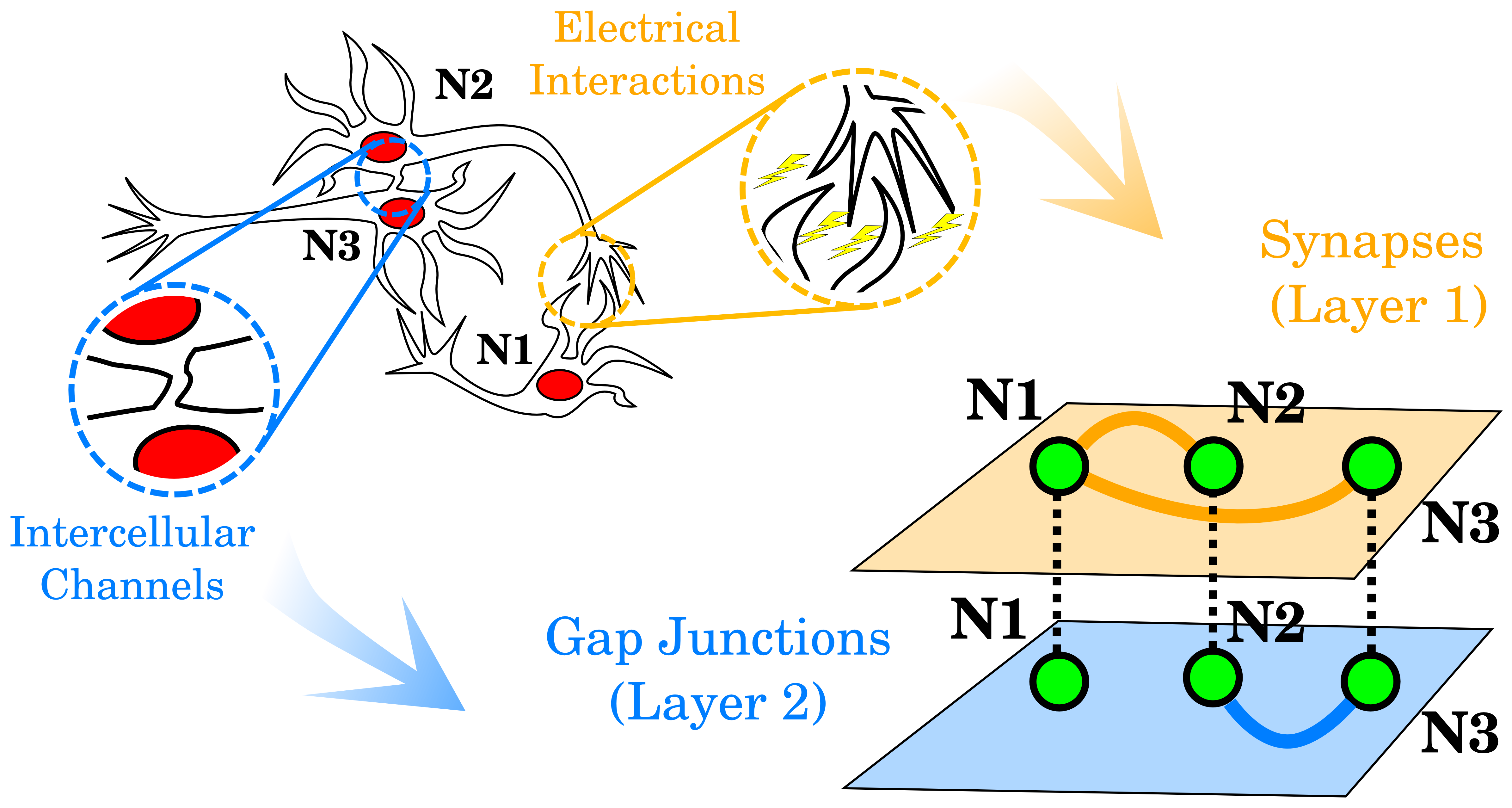
C.elegans. — The Caenorhabditis elegans is a small nematode, the first multicellular organism whose genome has been completely sequenced Celegans_genome . Thanks to the fact that its body is transparent, scientists have had the opportunity to study with unprecedented accuracy each and every cell of the C.elegans, and in particular its neural network, which is to date the only fully mapped brain of a living organism White1986 . The network, consisting of 281 neurons and around two thousands connections among them, was first analyzed as a complex network by Watts and Strogatz in their seminal paper on small-world networks Watts1998 , and has since then been thoroughly studied Latora2001 ; Arenas2008 ; NicosiaPNAS2013 . One important aspect of this network, which has been not considered in most of the analyses so far, is that the neurons can be connected either by a chemical link, a synapse, or by an ionic channel, the so-called gap junction. These two types of connection have completely different dynamics and function. Consequently, the neural network of the C.elegans can be naturally represented as a multiplex networks with $N=281$ nodes and two layers, respectively for synapses and gap junctions (see Fig. 1). Details of this multiplex, such as the number $N^{[\alpha]}$ of active nodes at each layer, i.e. nodes with at least one link at that layer, are shown in Table 2. In this particular network we have two layers, hence $\alpha=1$ or $\alpha=2$.

Genetic-Protein Network. — As another example of biological system we considered BIOGRID BIOGRID , a public database which collects and makes available for research genetic and protein interaction data from several organisms, including humans. The whole data set consists of around 500000 registered interactions among proteins in more than 40 different species. At the highest possible level, such interactions may be of two distinct types, namely physical and genetic. Two proteins A and B are said to interact physically if they can establish a physical contact to form a larger complex C, while they interact genetically if one of the two proteins, say A, regulates B, i.e. if A can trigger the activation (or repression) of the gene responsible for the production of B. It is worth mentioning that a more fine-grained classification of gene-protein interactions allows to identify up to seven different layers, as already shown in Refs. DeDomenico2015structural ; DeDomenico2014muxviz .

Also in this case, the research has been mostly focused on the study of the structural properties either of physical or of genetic interactions among proteins. We propose to study here the protein interaction networks as a multiplex network and, starting from the BIOGRID data set, we have constructed a network with two undirected and unweighted layers corresponding, respectively, to physical and genetic interactions among proteins. The resulting multiplex networks has $N=54549$ nodes, and the basic properties of the two layers are summarized in Table 2.

OpenFlight. — Another system which has been thoroughly investigated as a single-layer complex network is the airport transport system  Barrat2004 ; Colizza2006 . In this case the nodes of the network stand for airports and a link represents the existence of at least one direct flight between two airports. More fine-grained information about the airport transportation network has been recently made available Cardillo2013_Airports ; Cardillo2013_Emergence . Here we use a data set of aerial routes provided by OpenFlight OpenFlight , a collaborative free online tool which allows to map flights all around the world. Registered users of the website can upload information about their trips and share this information with friends. The maintainers of the website made available a dump of the data set which contains information about 59036 routes between 3209 airports operated by 531 different airlines spanning the whole globe. For each route we have information about the start point, the end point and the company which operates the flight. Starting from this data set, we constructed $6$ different multiplex networks. Each multiplex network represents the routes of a continent (Africa, Asia, Europe, North America, Oceania, South America) and consists of as many layers as airlines operating in that continent. The active nodes on each layer are the airports from which the corresponding airline company has at least one flight, and links represent the routes provided by that airline. In Table A-IV we report the basic features of each of the six continental multiplexes.

Network	M	$\bm{\eta}$	p-value
Africa	84	$1.64\pm 0.16$	0.20
Asia	213	$1.71\pm 0.12$	1.00
Europe	175	$1.48\pm 0.11$	0.11
North America	143	$1.52\pm 0.12$	0.99
Oceania	37	$1.37\pm 0.10$	0.04
South America	58	$1.58\pm 0.18$	0.90

Table A-IV: For each of the six continental airplane multiplex networks constructed from the OpenFlight database, we report the number of layers $M$ and the exponent $\eta$ of the distribution $P(N^{[\alpha]})\sim(N^{[\alpha]})^{-\eta}$ of the number of non-isolated nodes in each layer. The values of $\eta$ and the corresponding standard deviations were determined using the maximum likelihood estimator for power-law distributions Clauset2007 , while the p-value is based on the maximization of the Kolmogorov-Smirnov statistics over 1000 bootstrapped realizations (higher values of p-value are more significant).

APS Coauthorship. — Coauthorship networks are commonly constructed by connecting with an edge two researchers if they have published one or more papers together. We used a data set made available by the American Physical Society (APS) which reports information about all the papers published in any of the journals edited by APS since 1893 and up to 2009. In this data set, each paper published after 1975 is associated to up to four numeric codes, in the format XX.YY.ZZ, which identify a sub-field or research area according to the Physics and Astronomy Classification Scheme (PACS). At the highest level, PACS codes are organized into ten groups, respectively corresponding to sub-fields of physics. Starting from this data set, we constructed a multiplex collaboration network consisting of 10 layers, in which nodes represent authors and links connect authors having co-authored at least one paper. Authors with identical first and last name are considered the same authors. Please refer to Ref. disambiguation for a more comprehensive introduction on the problem of disambiguating authors in collaboration networks. Each layer corresponds to the collaborations identified by papers whose PACS codes are in one of the 10 high-level categories. In Table A-V we report the properties of the layers of this network. Each layer has up to around $79000$ active nodes, and the density varies across layers, according to the typical publication policy of each area of physics. For instance, papers in condensed matter and interdisciplinary physics are usually authored by just a few authors, while papers produced by large collaborations, including up to several hundred authors, are typical in particle physics, nuclear physics and astronomy.

Layer	Field	$N^{[\alpha]}$	$K^{[\alpha]}$	$\langle k^{[\alpha]}\rangle$
0	General	53170	1268045	47.7
1	Particles	37861	4865557	257.0
2	Nuclear	32792	1747892	106.6
3	Atomic	33649	189674	11.27
4	Classical	40269	222328	11.04
5	Gases and Plasmas	14237	179786	25.3
6	Condensed Matter I	63560	611765	19.3
7	Condensed Matter II	79416	631159	15.9
8	Interdisciplinary	45385	509058	22.4
9	Astronomy	31540	2467703	156.5
-	Aggregated	170397	6950611	81.6

Table A-V: The APS multiplex collaboration network consists of ten layers, one for each field of physics. For each layer $\alpha$ we report the number of active nodes $N^{[\alpha]}$, the number of edges $K^{[\alpha]}$ and the average degree $\langle k^{[\alpha]}\rangle$. We also report for reference the number of nodes, the number of edges and the average degree of the single-layer network obtained by aggregating all the layers.

IMDb. — The Internet Movie Database (IMDb) IMDb is a Web site providing comprehensive information about all the movie productions around the world. The data set is maintained and updated by volunteers, and made available for research use. It contains information about casts, producers, directors, etc. of several million movies belonging to 30 different genres. We constructed a multiplex network of collaborations among actors in which nodes represent actors and an edge exists between two nodes if the corresponding actors have co-acted in at least one movie. Each of the 30 categories represents a layer of the multiplex, so that if two actors have played a role in the same horror movie, they will be connected by an edge at the corresponding layer. In Table A-VI we show the basic characteristics of each layer of the multiplex. Notice that only 28 of the 30 layers are reported, since two of the layers, namely those corresponding to Experimental and Lifestyle movies, were deliberately left out of this study, since they contained less than 20 actors each. Notice also the wide variety of ranges in the number of active nodes. For instance Film-Noir has about 7 thousand active nodes, while Drama, have more than one million active nodes and more than 43 millions edges.

Layer	Genre	$N^{[\alpha]}$	$K^{[\alpha]}$	$\langle k^{[\alpha]}\rangle$
1	Action	330333	11800436	71.4
2	Adult	66756	1691208	50.7
3	Adventure	210293	7390148	70.3
4	Animation	55376	1120523	40.5
5	Biography	128552	4272197	66.5
6	Comedy	810693	30118775	74.3
7	Crime	297554	10051325	67.6
8	Documentary	313019	6850670	43.8
9	Drama	1091789	43352371	79.4
10	Family	198301	5432262	54.8
11	Fantasy	176080	5096872	57.9
12	Film-Noir	7035	399548	113.6
13	Game-Show	15222	282942	37.2
14	History	124803	4137162	66.3
15	Horror	263290	5428250	41.2
16	Musical	121471	4118346	67.8
17	Music	165110	4977063	60.3
18	Mystery	168898	4226618	50.0
19	News	21530	406166	37.7
20	Reality-TV	29112	465244	32.0
21	Romance	364042	13325687	73.2
22	Sci-Fi	164468	4147689	50.4
23	Short	644430	5117780	15.9
24	Sport	101006	3643330	72.1
25	Talk-Show	19700	516943	52.5
26	Thriller	356776	10757551	60.3
27	War	118960	3967033	66.7
28	Western	56638	2101057	74.2
-	Aggregated	2158300	$\sim 1.2\times 10^{8}$	$\sim 100$

Table A-VI: Basic features on each of 28 layers of the IMDb multiplex network and of the corresponding aggregated network. In this case, each layer corresponds to a movie genre.

References

- (1) M. E. J. Newman, “The structure and function of complex networks”, SIAM Review 45,, 167-256 (2003).
- (2) S. Boccaletti, V. Latora, Y. Moreno, M. Chavez and D.-U. Hwang, “Complex networks: structure and dynamics”, Phys. Rep. 424, 175 - 308 (2006).
- (3) D. J. Watts and S. H. Strogatz, “Collective dynamics of ’small–world’ networks”, Nature 393, 440–442 (1998).
- (4) A.-L. Barabasi and R. Albert, “Emergence of scaling in random networks”, Science 286, 509-512 (1999).
- (5) L. A. N. Amaral, A. Scala, M. Barthélémy and H. E. Stanley, “Classes of small–world networks”, Proc. Natl. Acad. Sci., USA 97, 11149-11152 (2000).
- (6) R. Pastor-Satorras, A. Vazquez and A. Vespignani, “Dynamical and correlation properties of the Internet”, Phys. Rev. Lett. 87, 258701 (2001).
- (7) R. Pastor-Satorras and A. Vespignani, “Epidemic spreading in scale–free networks”, Phys. Rev. Lett. 86, 3200 (2001).
- (8) V. Latora and M. Marchiori, “Efficient behavior of small–world networks”, Phys. Rev. Lett. 87, 198701 (2001).
- (9) M. E. J. Newman, “The structure of scientific collaboration networks”, Proc. Natl. Acad. Sci., USA 98, 404-409 (2001).
- (10) M. Girvan and M. E. J. Newman, “Community structure in social and biological networks”, Proc. Natl. Acad. Sci., USA 99, 7821-7826 (2002).
- (11) M. E. J. Newman, “Assortative mixing in networks”, Phys. Rev. Lett. 89, 208701 (2002).
- (12) A. Barrat, M. Barthelemy, R. Pastor-Satorras, A. Vespignani, “The architecture of complex weighted networks”, Proc. Natl. Acad. Sci. USA 101, 3747 (2004).
- (13) M. Szell, R. Lambiotte and S. Thurner, “Multirelational organization of large–scale social networks in an online world”, Proc. Natl. Acad. Sci., USA 107, 13636-13641 (2010).
- (14) A. Cardillo et al., “Emergence of network features from multiplexity”, Sci. Rep. 3, 1344 (2013).
- (15) A. Cardillo, M. Zanin, J. Gómez-Gardeñes, M. Romance, A. J. García del Amo, S. Boccaletti, “Modeling the Multi-layer Nature of the European Air Transport Network: Resilience and Passengers Re-scheduling under random failures” Eur. Phys. J. Spec. Top. 215, 23-33 (2013).
- (16) F. Battiston, V. Nicosia and V. Latora, “Structural measures for multiplex networks”, Phys. Rev. E 89, 032804 (2014).
- (17) M. De Domenico, A. Solé-Ribalta, E. Cozzo, M. Kivela, Y. Moreno, M. A. Porter, S. Gómez, A. Arenas, “Mathematical formulation for multi–layer networks”, Phys. Rev. X 3, 041022 (2013).
- (18) G. Menichetti, D. Remondini, P. Panzarasa, R. J. Mondragón, G. Bianconi, “Weighted multiplex networks”, PLoS ONE 9, e97857 (2014).
- (19) M. De Domenico, A. Solé-Ribalta, E. Omodei, S. Gómez, A. Arenas, “Ranking in interconnected multilayer networks reveals versatile nodes”, Nat. Commun. 6, 6868 (2015).
- (20) L. Solá, M. Romance, R. Criado, J. Flores, A. García del Amo, S. Boccaletti, “Eigenvector centrality of nodes in multiplex networks”, Chaos 23, 033131 (2013).
- (21) E. Cozzo, M. Kivelä, M. De Domenico, A. Solé, A. Arenas, S. Gómez, M. A. Porter, Y. Moreno, “Clustering coefficients in multiplex networks”, arXiv:1307.6780 (2013).
- (22) E. Estrada, J. Gómez-Gardeñes, “Communicability reveals a transition to coordinated behavior in multiplex networks”, Phys. Rev. E 89 042819 (2014).
- (23) B. Corominas-Murtra, B. Fuchs, S. Thurner, “Detection of the elite structure in a virtual multiplex social system by means of a generalized K-core”, PLoS ONE 9(12), e112606 (2014).
- (24) F. Radicchi, A. Arenas, “Abrupt transition in the structural formation of interconnected networks”, Nat. Phys. 9, 717-720 (2013).
- (25) G. Bianconi, S. N. Dorogovtsev, J. F. F. Mendes, “Mutually connected component of network of networks with replica nodes”, Phys. Rev. E 91, 012804 (2015).
- (26) G. Bianconi, “Statistical mechanics of multiplex networks: entropy and overlap”, Phys. Rev. E 87, 062806 (2013).
- (27) A. Halu, S. Mukherjee, G. Bianconi, “Emergence of overlap in ensembles of spatial multiplexes and statistical mechanics of spatial interacting networks ensembles”, Phys. Rev. E 89, 012806 (2014). (2013).
- (28) M. De Domenico, V. Nicosia, A. Arenas, V. Latora, “Structural reducibility of multilayer networks”, Nat. Commun. 6, 6864 (2015).
- (29) V. Nicosia, G. Bianconi, V. Latora and M. Barthélemy, “Growing multiplex networks”, Phys. Rev. Lett. 111, 058701 (2013).
- (30) J, Y. Kim and K.-I. Goh, “Coevolution and correlated multiplexity in multiplex networks”, Phys. Rev. Lett. 111, 058702 (2013).
- (31) V. Nicosia, G. Bianconi, V. Latora, M. Barthélemy, “Non-linear growth and condensation in multiplex networks”, Phys. Rev. E 90, 042807 (2014).
- (32) B. Fotouhi, N. Momeni, “Growing multiplex networks with arbitrary number of layers”, arXiv:1506.06278 (2015).
- (33) P. Klimek, S. Thurner, “Triadic closure dynamics explains scaling-exponents for preferential attachment-, degree- and clustering distributions in social multiplex data”, New J. Phys. 15 063008 (2013).
- (34) S. Gómez, A. Díaz-Guilera, J. Gómez-Gardeñes, C. J. Pérez-Vicente, Y. Moreno, A. Arenas, “Diffusion dynamics on multiplex networks”, Phys. Rev. Lett. 110, 028701 (2013).
- (35) M. De Domenico, A. Solé-Ribalta, S. Gómez, A. Arenas, “Navigability of interconnected networks under random failures”, Proc. Natl. Acad. Sci. USA 111(23), 8351–8356 (2014).
- (36) A. Solé-Ribalta, M. De Domenico, N. E. Kouvaris, A. Díaz-Guilera, S. Gómez, A. Arenas, “Spectral properties of the Laplacian of multiplex networks”, Phys. Rev. E 88 032807 (2013).
- (37) A. Halu, R. J. Mondragon, P. Panzarasa, G. Bianconi, “Multiplex PageRank”, PLoS ONE 8(10): e78293 (2013).
- (38) F. Battiston, V. Nicosia, V. Latora, “Biased random walks in multiplex networks”, arXiv:1505.01378 (2015)
- (39) C. Granell, S. Gómez, A. Arenas, “Dynamical interplay between awareness and epidemic spreading in multiplex networks”, Phys. Rev. Lett. 111 128701 (2013).
- (40) D. Zhao, L. Li, H. Peng, Q. Luo, Y. Yang, “Multiple routes transmitted epidemics on multiplex networks”, Phys. Lett. A378(10), 770-776 (2014).
- (41) A. Saumell-Mendiola, M. Á. Serrano and M. Boguñá, “Epidemic spreading on interconnected networks”, Phys. Rev. E 86, 026106 (2012).
- (42) C. Buono, L. G. Alvarez Zuzek, P. A. Macri, L. A. Braunstein, “Epidemics in partially overlapped multiplex networks”, PLoS ONE9(3), e92200 (2014).
- (43) B. Min, K.-I. Goh, “Layer-crossing overhead and information spreading in multiplex social networks”, arXiv:1307.2967 (2013).
- (44) E. Cozzo, R. A. Baños, S. Meloni, Y. Moreno, “Contact-based social contagion in multiplex networks”, Phys. Rev. E 89, 050801R (2013).
- (45) J. Gomez-Gardeñes, I. Reinares, A. Arenas and L. M. Floria, “Evolution of cooperation in multiplex networks”,Sci. Rep. 2, 620 (2012).
- (46) B. Min, S. Do Yi, K.-M. Lee, K.-I. Goh, “Network robustness of multiplex networks with interlayer degree correlations”, Phys. Rev. E 89, 042811 (2014).
- (47) L.-L. Jiang, M. Perc, “Spreading of cooperative behaviour across interdependent groups”, Sci. Rep. 3, 2483 (2013).
- (48) Z. Wang, A. Szolnoki, M. Perc, “Optimal interdependence between networks for the evolution of cooperation”, Sci. Rep. 3, 2470 (2013).
- (49) M. Diakonova, M. San Miguel, V. Eguiluz, “Absorbing and shattered fragmentation transitions in multilayer coevolution”, Phys. Rev. E 89, 062818 (2014).
- (50) A. Chmiel, K. Sznajd-Weron, “Phase transitions in the q-voter model with noise on a duplex clique”, arXiv:1503.01400 (2015).
- (51) F. Battiston, A. Cairoli, V. Nicosia, A. Baule, V. Latora, “Interplay between consensus and coherence in a model of interacting opinions”, arXiv:1506.04544 (2015).
- (52) M. Diakonova, V. Nicosia, V. Latora, M. San Miguel, “Irreducibility of multilayer network dynamics: the case of the voter model”, arXiv:1507.08940 (2015).
- (53) D. Cellai, E. López, J. Zhou, J. P. Gleeson, and G. Bianconi, “Percolation in multiplex networks with overlap”, Phys. Rev. E 88, 052811 (2013).
- (54) G. J. Baxter, S. N. Dorogovtsev, J. F. F. Mendes, D. Cellai, “Weak percolation on multiplex networks”, Phys. Rev. E89, 042801 (2014).
- (55) G. Bianconi, S. N. Dorogovtsev, “Multiple percolation transitions in a configuration model of network of networks”, Phys. Rev. E 89, 062814 (2014).
- (56) F. Radicchi, “Percolation in real interdependent networks”, Nat. Phys. 11, 597–602 (2015).
- (57) M. Kivela, A. Arenas, M. Barthélemy, J. P. Gleeson, Y. Moreno, M. A. Porter, “Multilayer networks”, J. Complex Net. 2, 203–271 (2014).
- (58) S. Boccaletti, G. Bianconi, R. Criado, C. del Genio, J. Gómez-Gardeñes, M. Romance, I. Sendiña-Nadal, Z. Wang, M. Zanin, “The structure and dynamics of multilayer networks”, Phys. Rep. 544(1), 1–122 (2014).
- (59) K.-M. Lee, B. Min, K.-I. Goh, “Towards real-world complexity: an introduction to multiplex networks”, Eur. Phys. J. B 88, 48 (2015).
- (60) R. Parshani, C. Rozenblat, D. Ietri, C. Ducruet, S. Havlin, “Inter-similarity between coupled networks”,EPL-Europhys. Lett. 92 68002 (2010).
- (61) K.-M. Lee, J. Y. Kim, W.-k. Cho, K.-I. Goh, and I.-M. Kim, “Correlated multiplexity and connectivity of multiplex random networks”, New J. Phys. 14, 033027 (2012).
- (62) http://www.maths.qmul.ac.uk/vnicosia
- (63) A. Clauset, C. R. Shalizi, M. E. J. Newman, “Power-law distributions in empirical data”, SIAM Review 51, 661–703 (2007).
- (64) R. Guimerá, L. A. N. Amarál, “Functional cartography of complex metabolic networks”, Nature 433, 895–900 (2005).
- (65) V. Colizza, A. Flammini, M.A. Serrano, A. Vespignani, “Detecting rich–club ordering in complex networks”, Nat. Phys. 2, 110 (2006).
- (66) D. Cellai, G. Bianconi, “Multiplex networks with heterogeneous activities of the nodes”, arXiv:1505.01220 (2015).
- (67) The C. elegans Sequencing Consortium ”Genome sequence of the nematode C. elegans: A platform for investigating biology”. Science 282(5396) 2012–2018 (1998).
- (68) J. G. White, E. Southgate, J. N. Thomson, S. Brenner, Phil. Trans. Royal Soc. London B, 314 (1165) 1-340 (1986).
- (69) A. Arenas, A. Fernández and S. Gómez, “Bio-Inspired Computing and Communication” Lect. Notes Comp. Sci., 5151, 9-18 (2008).
- (70) V. Nicosia, P. Vertés, W. Schafer, V. Latora, E. Bullmore, “Phase transition in the economically modeled growth of a cellular nervous system”, Proc. Natl. Acad. Sci., USA 110(19), 7880-7885 (2013).
- (71) C. Stark, B.J. Breitkreutz, T. Reguly, L .Boucher, A. Breitkreutz, M. Tyers, Nucleic Acids Res. Jan1; 34:D535-9 (2006).
- (72) M. De Domenico, M. A. Porter, A. Arenas, “MuxViz: a tool for multilayer analysis and visualization of networks”, J. Complex Net. 3, 159–176 (2015).
- (73) http://openflight.org
- (74) J. Kim, J. Diesner, “Distortive effects of initial-based name disambiguation on measurements of large-scale coauthorship networks”, J. Assn. Inf. Sci. Tec. doi:10.1002/asi.23489 (2015).
- (75) http://www.imbd.com