Reionization and CMB non-Gaussianity

Abstract

We show how cross-correlating a high redshift external tracer field, such as the 21cm neutral hydrogen distribution and product maps involving Cosmic Microwave Background (CMB) temperature and polarisation fields, that probe mixed bispectrum involving these fields, can help to determine the reionization history of the Universe, beyond what can be achieved from cross-spectrum analysis. Taking clues from recent studies for the detection of primordial non-Gaussianity (Munshi & Heavens, 2010), we develop a set of estimators that can study reionization using a power spectrum associated with the bispectrum (or skew-spectrum). We use the matched filtering inherent in this method to investigate different reionization histories. We check to what extent they can be used to rule out various models of reionization and study cross contamination from different sources such as the lensing of the CMB. The estimators can be fine-tuned to optimize study of a specific reionization history. We consider three different types of tracers in our study, namely: proto-galaxies; 21cm maps of neutral hydrogen; quasars. We also consider four alternative models of reionization. We find that the cumulative signal-to-noise (S/N) for detection at $\ell_{max}=2000$ can reach $\mathcal{O}(70)$ for cosmic variance limited all-sky experiments. Combining 100GHz, 143GHz and 217GHz channels of the Planck experiment, we find that the (S/N) lies in the range $\mathcal{O}(5)-\mathcal{O}(35)$. The (S/N) depends on the specific choice of a tracer field, and multiple tracers can be effectively used to map out the entire reionization history with reasonable S/N. Contamination from weak lensing is investigated and found to be negligible, and the effects of Thomson scattering from patchy reionization are also considered.

1 Introduction

Pinning down the details and controlling physics of the cosmological reionization history remains one of the important goals of present-day cosmology. It is well known, thanks to a large set of astrophysical observables, that after primordial recombination, which occurred at a redshift of $z\sim 1100$, the Universe reionized at a redshift $z>6$. The epoch-of-reionization (EoR) is related to many fundamental questions in cosmology, such as the properties of the first galaxies, physics of (mini-)quasars, formation of very metal-poor stars and a slew of other important research topics in astrophysics. Hence uncovering it will have far reaching implications on the study of structure formation in the early Universe (Loeb & Barkana, 2001). Observations of Lyman-$\alpha$ forests with high-resolution echelle spectrographs on large telescopes (such as HIRES on Keck, and UVES on ESO’s Very Large Telescope) are valuable for studying reionization at $z\approx 2.5-6.5$ (Fan et al., 2006; Fax, Carli & Keating, 2006). Redshifted 21cm observations are also a very important probe of the EoR and several instruments are either operational or in the construction phase. In the short term these consists of: The Low Frequency Array (LOFAR), the Murchison Widefield Array (MWA), Precision Array to Probe Epoch of Reionization (PAPER) and Giant Metrewave Radio Telescope (GMRT), while, on a somewhat longer time scale the Square Kilometre Array (SKA) will be operational.

In addition to Lyman-$\alpha$ and 21cm redshifted observations, CMB temperature and polarisation studies can also provide valuable information regarding the EoR. The polarisation signal in CMB is generated due to the scattering of the local CMB temperature quadrupole by the free-electron population. This signal peaks at angular scales corresponding to the horizon at the rescattering surface (at a few tens of degrees) and the amplitude depends on total optical depth. However, the large cosmic variance associated with the signal means it is impossible to discriminate among various reionization histories using cross-correlation of the CMB temperature and polarisation (Kaplinghat et al., 2003; Holder et al., 2008; Hu & Holder, 2008). The total optical depth to reionization using WMAP data is $\tau=0.08\pm 0.013$ (Bennett et al., 2013). Most current constraints from CMB data are analysed assuming a “sudden” and complete reionization at a redshift $z_{r}$ for WMAP this value of $\tau$ will correspond to $z_{r}=11$. However as mentioned before, the precise details of the reionization process are not very well known and clearly the reionization history of the universe at those redshifts could have easily been very different. The combination of temperature data and lensing reconstruction from the Planck data gives an optical depth $\tau=0.089\pm 0.032$ (Planck Collaboration, 2013d), consistent with WMAP9 estimates. The polarization data from Planck is expected to improve the accuracy of determination of $\tau$, however, it is important to keep in mind that CMB observations only provide integrated or projected information on reionization.

The process of reionization is expected to be patchy and inhomogeneous in scenarios where reionization is caused by UV emission from the first luminous objects (e.g. Meerburg, Dvorkin & Spergel, 2013), and the resulting fluctuations in visibility will generate extra anisotropy at arcminute scales. Even in scenarios when reionization is caused by energy injection from decaying particles or X-ray emission, inhomogeneities in electron density can cause fluctuations in visibility, but these fluctuations are too small to be detected in temperature and polarization power spectra or their cross-spectrum. Nevertheless, as one can imagine, additional signals due to inhomogeneneites in the free-electron density may imprint additional features at smaller angular scales (Hu, 2008; Santos et al., 2003), and the mixed bispectrum with external data sets was advocated to extract redshift information (Cooray, 2004; Alvarez et al., 2006; Adshead & Furlanetto, 2007; Tashiro et al., 2010; Holder, Iliev & Mellama, 2007).

In fact, what is required is the three-point correlation (or equivalently the bispectrum) involving temperature, polarisation and a tracer field for the free electron population can extract useful information on the ionization history of the Universe (Cooray, 2004). For details of the generation of secondary non-Gaussianity due to reionization see (Khatri & Wandelt, 2010).

The estimation of the bispectrum is a lot more complicated than the power spectrum due to the presence of additional degrees of freedom. As has been pointed out in many recent works, the mode-by-mode estimation of the bispectrum, though very attractive, is seldom useful because of the associated low signal-to-noise (e.g. Bartolo et al., 2004, for a review). Typically, this means, the entire information content of the bispectrum is often compressed into a single number which is used to distinguish various models of reionization. Though this has the advantage of increasing the (S/N), it also degrades the information content of the bispectrum.

A compromise solution was proposed recently by Munshi & Heavens (2010), who defined a power spectrum associated with a specific bispectrum. This power spectrum represents the cross-spectra of the product of two maps $[\rm X(\hat{\bf\Omega})Y(\hat{\bf\Omega})]$ against another map $\rm Z(\hat{\bf\Omega})$. It is a weighted sum of individual modes of the bispectrum keeping one of the index fixed while summing over the other two indices. Such an estimator can also be designed to work with an experiential mask for estimation in the presence of non-uniform noise and is relatively simple to implement. In the literature such estimators are known as pseudo-${\cal C}_{\ell}$ (PCL) estimators. However, such estimators are sub-optimal. With the recent attempts to detect primordial non-Gaussianity in the aftermath and leading up to the Planck data release (Planck Collaboration, 2013a, b) there has been an increased activity in the area of optimising estimators which can probe primordial non-Gaussianity (Heavens, 1998; Komatsu, Spergel & Wandelt, 2005; Creminelli et al., 2006; Creminelli, Senatore, & Zaldarriaga, 2007; Smith, Zahn & Dore, 2000; Smith & Zaldarriaga, 2006). Detection of secondary non-Gaussianity, can also benefit from using the Munshi & Heavens (2010) estimators to take into account inhomogeneous noise and partial sky coverage in an optimal way (Munshi et al., 2011). We will discuss these issues and other related optimisation problems in this paper for mixed data sets. Being able to probe the bispectrum in a scale-dependent way will provide a useful way to differentiate among different theories of reionization. The matched filtering inherent in these estimators are likely to be very useful in pinning down a specific reionization history. The formalism also provides a natural set-up to study cross-contamination from effects of weak lensing. The approach presented here has already been successfully implemented for Planck data analysis which resulted in the detection of non-Gaussianity from the correlation of the Integrated Sachs-Wolfe (ISW) effect with gravitational lensing, and from residual point sources in the maps (Planck Collaboration, 2013b).

We will define several set of different estimators. In addition to using the direct estimators, we will define, three dimensional constructs that require the use of appropriate weight functions to cross-correlate and probe the secondary non-Gaussianity. We will also point to computationally extensive estimators which can take into account all possible complications. These generalisations involve a set of fully optimal estimators which can work directly with harmonics of associated fields and carry out inverse covariance weighting using a direct brute force approach. Clearly, though such a direct approach is completely optimal it is prohibitively expensive to implement beyond a certain resolution. Nevertheless, for secondary bispectrum which we consider here, it will be important to maintain the optimality to a high resolution as most relevant information will be appear on small scales.

The results presented here can be seen as an extension of our earlier papers: for example, (Munshi & Heavens, 2010), where we presented skew-spectrum for primary non-Gaussianity; (Munshi et al., 2011), where results relevant to secondary non-Gaussianity were obtained. Here, we include polarization data in addition to the temperature maps and cross-correlate with external data sets in 3D to constrain various scenarios of reionization. In recent years we have extended the concept of skew-spectra to study topological properties of CMB maps (Munshi, Coles & Heavens, 2013a; Munshi et al., 2013b) as well as for other cosmological data sets such as frequency-cleaned thermal Sunyaev Zeldovich $y$-maps (Munshi et al., 2012a) or weak lensing maps (Munshi et al., 2012b).

This paper is organised as follows: In §2.1 we present many of our analytical results and include the description of reionization models and the tracer fields that we study. We introduce our estimators in §3. In §4 we discuss our results and §5 is devoted to concluding remarks. In Appendix A we outline how a skew-spectrum estimator can be constructed using minimum variance estimated of fluctuations in optical depth. In Appendix B we provide equivalent estimators for the reconstruction of the lensing potential.

2 Notations and Analytical Results

2.1 Mixed Bispectrum

Given a bispectrum involving three different fields $\rm X(\hat{\bf\Omega})$, $\rm Y(\hat{\bf\Omega})$ and $\rm Z(\hat{\bf\Omega})$, we can define a mixed bispectrum $B^{\rm XYZ}_{\ell_{1}\ell_{2}\ell_{3}}$ which encodes non-Gaussianity at the three-point level (see Munshi & Heavens (2010) for more discussion regarding definitions related to the bispectrum and its estimation).

$$\langle{\rm X}_{\ell_{1}m_{1}}{\rm Y}_{\ell_{2}m_{2}}{\rm Z}_{\ell_{3}m_{3}}\rangle_{c}=\sum_{m_{1}m_{2}m_{3}}B_{\ell_{1}\ell_{2}\ell_{3}}^{\rm XYZ}\left(\begin{array}[]{ c c c }\ell_{1}&\ell_{2}&\ell_{3}\\ m_{1}&m_{2}&m_{3}\end{array}\right);\qquad{\rm X,Y,Z}={(\Theta,E,S)}~{}{\rm or}~{}{(\Theta,B,S)}.$$ (1)

The matrices here represent 3j symbols (Edmonds, 1968) and reflect the rotational invariance of the three-point correlation function. We will specialize our discussion later to the case of cross-correlating temperature $\Theta$, polarisation fields ($E\pm iB$) with a tracer field $S$ that traces the fluctuations in the free electron density. The secondary polarisation is generated by rescattering of CMB photons at a much lower redshift than decoupling.

The polarisation field is

$$P_{\pm}(\hat{\bf\Omega})=(q\pm iu)(\hat{\bf\Omega})={\sqrt{24\pi}\over 10}\int drg(r)\sum_{m=-2}^{2}\delta\Theta_{2m}({\bf x}){}_{\pm 2}Y_{2m}(\hat{\bf\Omega});\\ \quad\quad\delta\Theta_{2m}=-{1\over 4\pi}\int d\hat{\bf\Omega}Y_{2m}\delta\Theta_{2m}({\bf x},\hat{\bf\Omega});$$ (2)

with

$$g(r)\equiv\dot{\tau}(r)\exp[{-\tau(r)}]=x_{\rm e}(z){H}_{0}\tau_{\rm H}(1+z)^{2}\exp({-\tau});\qquad\tau(r)=\int_{0}^{r}dr^{\prime}\;\dot{\tau}(r^{\prime});\qquad\tau_{\rm H}=0.0691(1-Y_{\rm p})\Omega_{b}h.$$ (3)

Here $g(r)$ is the visibility function which represents the probability of an electron being scattered within a distance $dr$ of $r$; $\tau(r)$ is the optical depth out to distance $r$ with $\tau_{H}$ denoting the optical depth to the Hubble distance today due to Thomson scattering, which assumes full hydrogen ionization and a primordial helium fraction $Y_{\rm p}=0.24$; $x_{\rm e}(z)$ is the ionization fraction as a function of redshift $z$. The conformal distance $r$ at redshift $z$ is given in terms of the Hubble parameter as $r(z)=\int_{0}^{z}{dz^{\prime}/H(z^{\prime})}$ with $H^{2}(z)=H_{0}^{2}[\Omega_{\rm M}(1+z)^{3}+\Omega_{\rm K}(1+z)^{2}+\Omega_{\Lambda}]$, parametrised in terms of the total cosmic matter density (cold dark matter + baryons) $\Omega_{\rm M}=\Omega_{c}+\Omega_{b}$, the cosmological constant density $\Omega_{\rm\Lambda}$ and the curvature $\Omega_{\rm K}=(1-\Omega_{\rm M}-\Omega_{\Lambda})$ in units of the critical density $3{\rm H}_{0}^{2}/8\pi\,G$. Here $H_{0}^{-1}=2997.9h^{-1}$Mpc is the inverse Hubble distance with $h=H_{0}/100$. In the following we will assume a standard flat LCDM cosmological model with $\Omega_{c}=0.30$, $\Omega_{b}=0.05$, $\Omega_{\Lambda}=0.65$ and $h=0.65$ respectively.

The primary effect of reionization is manifested by the suppression of the temperature power-spectrum ${\cal C}^{\Theta\Theta}_{\ell}$ by a factor $\exp(-2\tau)$ and enhancement of ${\cal C}^{\rm EE}_{\ell}$ power spectrum at small $\ell$ which scales as $\tau^{2}$. Most CMB calculations adopt an abrupt reionization. However low redshift studies involving Lyman-$\alpha$ optical depth related Gunn-Peterson troughs of the $z\sim 6$ quasars indicate a more complex reionization history; moreover the reionization can be patchy or inhomogeneous (Barkana & Loeb, 2001).

The mixed bispectrum $B_{\ell_{1}\ell_{2}\ell}^{S\Theta E}$ can be written as:

$$B_{\ell_{1}\ell_{2}\ell}^{E\Theta S}=\sqrt{\Sigma_{\ell_{1}}\Sigma_{\ell_{2}}\Sigma_{\ell}\over 4\pi}\left(\begin{array}[]{ c c c }\ell_{1}&\ell_{2}&\ell\\ 0&0&0\end{array}\right)b^{E}_{\ell_{2}\ell_{1}};\quad\quad\Sigma_{\ell}\equiv(2\ell+1),$$ (4)

where $b^{E}_{\ell_{2}\ell_{1}}$ is the reduced bispectrum, using the Limber’s approximation the latter reads as (see Cooray, 2004, for derivation and detailed discussion):

$$b^{E}_{\ell_{2}\ell_{3}}={2\over 9\pi}\int dr\;g(r)\;{G^{2}(r)\over d_{A}^{2}(r)}W_{S}(r)P_{gS}\left(k={\ell_{3}\over d_{A}}\right){\cal I}_{l_{2}}^{E}(r);\qquad{\cal I}_{\ell}^{E}(r)=\int k^{2}dkP_{\Phi\Phi}(k,r_{0})j_{\ell}(kr_{0})j_{2}(kr_{s})\epsilon^{E}_{\ell}(kr);\quad\quad$$ (5)

$$r_{s}\equiv r-r_{0};\quad\quad r_{0}=r\,(z=1100);$$ (6)

where $\epsilon_{\ell}^{E}(kr)$ can be written in terms of the spherical Bessel function $j_{\ell}(x)$ and its derivatives $j^{\prime}_{\ell}(x)$ and $j^{\prime\prime}_{\ell}(x)$:

$$\epsilon_{\ell}^{E}(x)=-j_{\ell}(x)+j_{\ell}^{\prime\prime}(x)+2j_{\ell}(x)/x^{2}+4j_{\ell}^{\prime}(x)/x.$$ (7)

In the above expression $d_{A}(r)=H_{0}^{-1}\Omega_{\rm K}\sinh[H_{0}\Omega_{\rm K}^{1/2}r]$ is the angular diameter distance which in a flat universe ($\Omega_{K}\rightarrow 0$) reduces to $d_{A}(r)\rightarrow r$. $W_{S}(r)$ represents the spatial distribution of the tracers and $G(r)$ is the linear growth factor defined such that the Fourier transform of the overdensity field grows as $\delta({\bf k},r)=G(r)\delta({\bf k},0)$ given by:

$$G(r)={H(z)\over H_{0}}\int_{z(r)}^{\infty}dz^{\prime}(1+z^{\prime})\left[H(z^{\prime})\right]^{-3}\Big{/}\int_{0}^{\infty}dz^{\prime\prime}(1+z^{\prime\prime})\left[H(z^{\prime\prime})\right]^{-3},$$ (8)

which we compute using a standard numerical integration algorithm.

Throughout we will be using the normalisation $\langle\Phi({\bf k})\Phi({\bf k^{\prime}})\rangle=(2\pi)^{3}\delta^{D}({\bf k}+{\bf k^{\prime}})P_{\Phi\Phi}(k)$ for the power spectrum $P_{\Phi\Phi}(k)$ of the primordial potential perturbation $\Phi$ and $\langle\delta_{g}({\bf k})\delta_{S}({\bf k^{\prime}})\rangle=(2\pi)^{3}\delta^{D}({\bf k}+{\bf k^{\prime}})P_{gS}(k)$, where $P_{gS}(k,z)$ is the cross-spectrum at a redshift $z$ between fluctuations in the scattering visibility function and the tracer field. In the following we assume a halo model such that $P_{gS}(k,z)=b_{g}(z)b_{S}(z)G^{2}(z)P^{\rm L}_{\delta\delta}(k)$ where $b_{g}(z)$ and $b_{S}(z)$ are the biases at large scales of the underlying fields and $P^{\rm L}_{\delta\delta}(k)$ is the linear matter power spectrum given by:

$$P_{\delta\delta}^{\rm L}(k)=2\pi^{2}A_{s}\left(\frac{k}{k_{p}}\right)^{n_{s}-1}k\,T^{2}(k),$$ (9)

where $A_{s}$ is the scalar amplitude, $n_{s}$ is the scalar spectral index, $k_{p}=0.05$ Mpc^-1 the pivot scale and $T(k)$ is the CDM transfer function which we compute from (Eisenstein & Hu, 1998). We assume $n_{\rm s}=0.9635$ and $A_{\rm s}=2.19\times 10^{-19}$. We will use these results to construct estimators based on the PCL approach or near optimal estimators based on generalisation of Munshi & Heavens (2010).

2.2 Tracer Distribution Models

We consider three different tracer sources corresponding to a population of proto-galaxies contributing to the IR background (a), 21cm-like tracers (b) and a quasar-like sources (c). In the case of tracer model (a) and (b) we assume a Gaussian redshift distribution:

$${\rm Model\;(a)\;and\;(b)}:W(z)={1\over\sqrt{2\pi\sigma_{z}^{2}}}\exp\left[-{1\over 2}{(z-\bar{z})^{2}\over\sigma_{z}^{2}}\right].$$ (10)

with parameters $\bar{z}=15$ and $\sigma_{z}=3$ for (a) and $\bar{z}=20$ and $\sigma_{z}=1$ for (b). In the case of quasar-like sources (c) we assume a broad redshift distribution

$${\rm Model\;(c)}:W(z)=\left({z\over{\bar{z}}}\right)^{\alpha}\left({\beta\over{\bar{z}}}\right)\exp\left[-\left({z\over{\bar{z}}}\right)^{\beta}\right].$$ (11)

with parameters $\bar{z}=3$, $\alpha=2$ and $\beta=1.5$. The normalised redshift distributions of the tracer fields are plotted in Fig. 2 (right-panel).

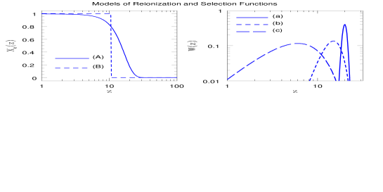
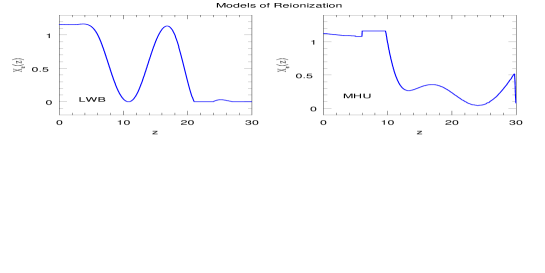
Figure 1: Left panel: ionization fraction $x_{\rm e}(z)$ for slow or smooth (A) and sudden (B) reionization models (see text). Right panel: redshift distribution of sources $W(z)$ for three different populations of tracers corresponding to proto-galaxies (a), 21cm-emitters (b) and quasar-like sources (c).

Figure 2: Ionization fraction $x_{\rm e}(z)$ for two different non-standard reionization models denoted as LWB (Lewis, Weller & Battye, 2006) (left panel) and MHU (Mortonson & Hu, 2008) (right panel). In the case of LWB a binned ionization history was considered, while a Principle Component Analysis (PCA) was employed in MHU.

2.3 Reionization Models

In order to test the potential of testing the reionization history through mixed bispectrum analyses we focus on different reionization history models which are indistinguishable from one another using CMB temperature, polarization and their cross-correlation spectra. These models are characterized by differention redshift dependencies of the ionization fraction:

$$\quad{\bf{\rm\underline{Model\;(A)}}}\;\;({\rm or\;the\;smooth\;model}):x_{\rm e}(z)=1-{1\over 2}{\rm Erfc}\left[{(z_{r}-z)\over\sigma_{z}}\right];\quad\quad z_{r}=15,\quad\sigma_{z}=7.5;$$ (12)

$$\quad{\bf{\rm\underline{Model\;(B)}}}\;\;({\rm or\;the\;sharp\;model}):x_{\rm e}(z)=\begin{cases}1&\text{if $z<z_{r}$}\\ 0&\text{otherwise}\end{cases};\quad\quad z_{r}=11.35$$ (13)

Model (LWB): this is double reionization scenario studied in Lewis, Weller & Battye (2006) which we implement by considering 12 redshift bins centered at $z={0,3,6,9,12,15,18,21,24,27,30,32}$ with values of $x_{\rm e}={1.16,1.16,1.0,0.2,0.1,0.9,1.0,0.002,0.002,0.002,0.002,0.002}$ respectively which we use to built a cubic spline interpolation of $x_{e}(z)$. The values of $x_{e}$ in the first two redshift bins take into account the effect of second helium reionization, while the third one only has the contribution from first hydrogen reionization. The total optical depth for this model is 0.14. For $z>18$ we set $x_{e}=2\times 10^{-4}$ which is the value of $x_{e}$ expected before reionization (following primordial recombination).

Model (MHU): this reionization scenario has been studied in (Mortonson & Hu, 2008) and is based on a parametrized reionization history built by decomposing $x_{e}(z)$ into its principal components $x_{e}(z)=x_{e}^{\rm fid}(z)+\sum_{\mu}m_{\mu}S_{\mu}(z)$, where the principal components, $S_{\mu}(z)$, are the eigenfunctions of the Fisher matrix that describes the dependence of the $C_{\ell}^{\rm EE}$ on $x_{e}(z)$, $m_{\mu}$ are the amplitudes of the principal components for a given reionization history, and $x_{e}^{\rm fid}(z)$ is the fiducial model at which the Fisher matrix is computed. For the MHU model we have used the first five principal components for the reconstruction of the reionization history (for more details see Pandolfi et al., 2010). The values of amplitudes are consistent with the one-sigma confidence level values around the best fit obtained using Planck data (Planck Collaboration, 2013c). The total optical depth for this model is $\tau=0.15$.

The smooth model (A) corresponds to reionization by UV light from star forming regions within collapsed halos (Cooray, 2004), while the instantaneous transition model (B) to a fully reionised Universe from a neutral one could arise e.g. in the presence of X-ray background (Oh, 2001) or from decaying particles (Hansen & Haiman, 2004; Chen & Kamionkowski, 2004; Kasuya, Kawasaki & Sugiyama, 2004). The redshift evolution of the ionization fraction for models (A) and (B) is shown in Fig. 2 (left-panel), while in Fig. 2 we plot the ionization fractions of LWB (left-panel) and MHU (right-panel).

In Fig. 4 and 4 we plot the temperature ${\cal C}^{\rm TT}_{\ell}$ (left panel), E-polarization ${\cal C}^{\rm EE}_{\ell}$ (middle panel) and cross temperature-polarization spectra ${\cal C}^{\rm T\rm E}_{\ell}$ (right panel) for the different reionization history models. We can see that despite the different redshift dependence of the ionization fraction these models are indistinguishable using only CMB measurements.

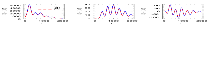
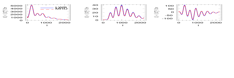
Figure 3: The CMB temperature power spectrum ${\cal C}^{\rm TT}_{\ell}$ (left panel), Electric or E-type polarization power-spectra ${\cal C}^{\rm EE}_{\ell}$ (middle panel) and temperature-polarization cross-spectrum ${\cal C}^{\rm T\rm E}_{\ell}$ (right panel) for models (A) “slow” and (B) “sudden”.

Figure 4: As in Fig. 4 for LWB and MHU models respectively.

We compute the reduced bispectrum for the different reionization history models using Eq. (6), for simplicity we set the bias functions $b_{g}(z)=b_{S}(z)=1$. In Fig. 5 we plot $b_{\ell_{2}\ell_{3}}$ as function $\ell_{2}$ at constant $\ell_{3}=10,100,100$, while Fig. 6 we plot $b_{\ell_{2}\ell_{3}}$ as function $\ell_{2}$ at constant $\ell_{3}=10,100,100$. We can see that differently from the CMB spectra the different models gives different predictions for the amplitude of the reduced bispectrum. Furthermore they show that information is encoded in the multipole structure of $b_{\ell_{2}\ell_{3}}$. As one may expected the overall amplitude of the signal depends on how well the tracers overalp with a non-vanishing value of the ionization fraction. In other words the larger the redshift interval where the convolution of the tracer distribution with the visibility function is non-vanishing and the larger is the signal. As an example let us look at the reduced bispectrum at constant $\ell_{3}$ values for the “slow” and “sudden” reionization models shown in two top-panels of Fig. 5. In the “sudden” case the visibility function vanishes at $z>11.35$, this implies that fluctuations of high-redshift tracer fields such as model (a) will be less correlated with fluctuations of the visibility function and the large angular scale polarization pattern of the CMB. In contrast, in the “slow” model the visibility function is still non-vanishing at high-redshift thus leading to a larger value of the reduced bispectrum. The multipole structure of the reduced bispectrum at constant $\ell_{2}$ values depends on the specific reionization model and the tracer field and it is harder to disentangle since other factors such as the projected matter power spectrum, the amplitude of the tracer distribution (i.e. the abundance of sources), the specific redshift evolution of the visibility function comes into play. Nevertheless, it is worth noticing that the amplitude changes between positive and negative values at different values of $\ell_{2}$. This is because the integral ${\cal I}_{l_{2}}^{E}(r)$ in Eq. (6) oscillates as function of $\ell_{2}$ and as we can see in Fig. 6 the change of sign depends on the reionization model. Overall, this suggests that the bispectrum of fields which correlates with reionization history carries a distinctive imprint of this process. In the next sections we will assess the detectability of such signal for Planck-like experiments using skew-spectra.

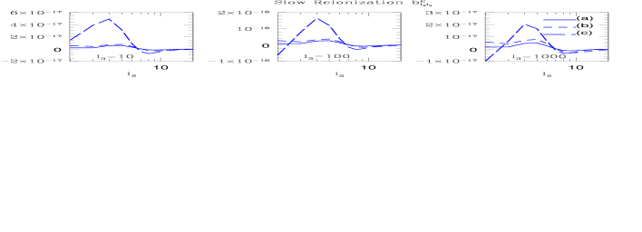
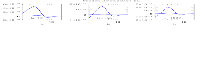
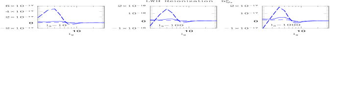
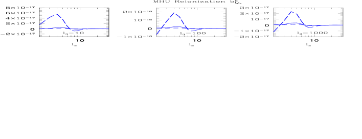
Figure 5: Reduced bispectrum as function of $\ell_{2}$ at constant $\ell_{3}=10,100,1000$ for different reionization history models.

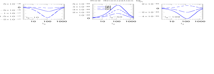
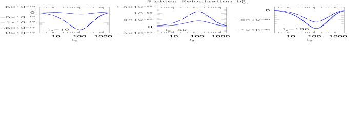
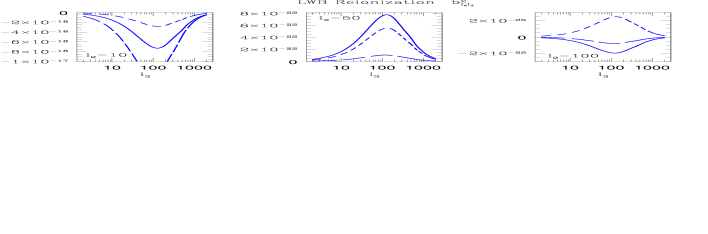
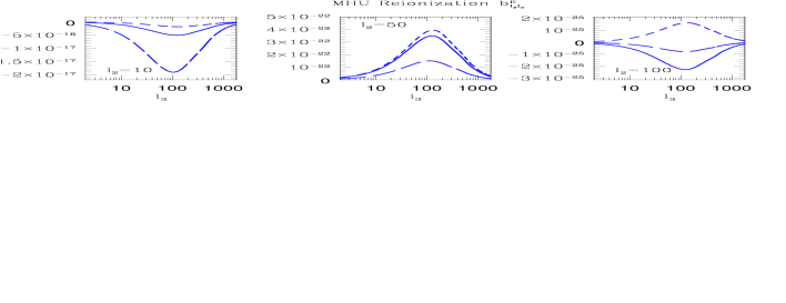
Figure 6: Reduced bispectrum as function of $\ell_{3}$ at constant $\ell_{2}=10,50,100$ for different reionization history models.

3 Estimators

In this section we will introduce the estimators for our skew-spectra. We first discuss the direct PCL estimator which is sub-optimal. Next we introduce the near-optimal skew-spectra that involves constructing 3D fields with appropriate weights. We will also discuss contamination from CMB lensing. The estimators presented here will be useful in probing patchy reionization scenarios.

3.1 Direct or Pseudo-${\cal C}_{\ell}$ Approach

In principle it is useful to study the bispectrum for every possible triplet of $(\ell_{1},\ell_{2},\ell_{3})$ represented by triangular configuration in the harmonic space. However, this is a challenging task due to the low signal-to-noise associated with individual modes. The usual practice is to sum all possible configurations and study the resulting skewness. However, this method of data compression is extreme and a trade-off can be reached by summing over two specific indices while keeping the other fixed. In real space this is equivalent to cross-correlating the product field $[{\rm X}(\hat{\bf\Omega}){\rm Y}(\hat{\bf\Omega})]$ against ${\rm Z}(\hat{\bf\Omega})$. The resulting power spectrum (called the skew spectrum) can be studied as a function of $\ell$. The usual skewness then can be expressed as a weighted sum of this skew-spectrum. In a recent work, Munshi & Heavens (2010) proposed a power-spectrum associated with a given bispectrum. This encodes more information compared to the one-point skewness often used in the literature. A PCL approach or its variants in real or harmonic space has been used in many areas, for analysing auto or mixed bispectrum from diverse dataset (Munshi et al., 2011):

$${\cal C}_{\ell}^{\rm XY,Z}=\sum_{\ell_{1}\ell_{2}}B_{\ell\ell_{1}\ell_{2}}^{\rm XYZ}\sqrt{\Sigma_{\ell_{1}}\Sigma_{\ell_{2}}\over\Sigma_{\ell}}\left(\begin{array}[]{ c c c }\ell&\ell_{1}&\ell_{2}\\ 0&0&0\end{array}\right);\qquad{\rm X,Y,Z}=(\Theta,{\bf E},{\bf S})\;or\;(\Theta,{\bf B},{\bf S}).$$ (14)

The different power spectra associated with this bispectrum correspond to various choices of two fields $\rm X$ and $\rm Y$ to correlate with the third field $\rm Z$. We can construct three different power spectra related to this given bispectra.

$${\cal C}_{\ell}^{S\Theta,E}=\sum_{\ell_{1}\ell_{2}}J_{\ell_{1}\ell_{2}\ell}[b^{E}_{\ell_{2}\ell_{1}}];\qquad{\cal C}_{\ell}^{SE,\Theta}=\sum_{\ell_{1}\ell_{3}}J_{\ell_{1}\ell\ell_{3}}[b^{E}_{\ell\ell_{1}}];\qquad{\cal C}_{\ell}^{E\Theta,S}=\sum_{\ell_{2}\ell_{3}}J_{\ell\ell_{2}\ell_{3}}[b^{E}_{\ell_{2}\ell}];\qquad$$ (15)

$$J_{\ell_{1}\ell_{2}\ell}=\left({\Sigma_{\ell_{1}}\Sigma_{\ell_{2}}\over 4\pi}\right)\left(\begin{array}[]{ c c c }\ell_{1}&\ell_{2}&\ell\\ 0&0&0\end{array}\right)^{2}.$$ (18)

Similar results will hold for expressions involving B-type polarisation. The advantage of using a PCL approach is related to the fact that it does not depend on detailed modelling of the target theoretical model. It is extremely fast and is only limited by the speed of harmonic transforms. In Fig. 7 we plot the PCL skew-spectra for different reionization history models. Here, we can see more clearly the dependence of the amplitude of the skew-spectra on the redshift distribution of the tracers discussed in the previous section.

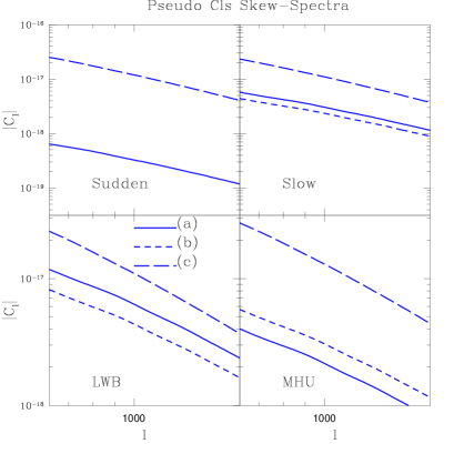
Figure 7: The pseudo-${\cal C}_{\ell}$ (PCL) estimator ${\cal C}^{\Theta\rm E,X}_{\ell}$ defined in Eq. (14) for various models of reionization: “slow” (upper-right panel), “sudden” (upper-left panel), LWB (lower-left panel) and MHU (lower-right panel). For each model we plot the PCL for the tracer model (a) (solid line), model (b) (short-dashed line) and model (c) (long-dashed line) respectively.

3.2 Defining optimal weights and Near-Optimal Esimators

The weights required for the construction of an optimal estimator need the theoretical modelling of the bispectra that is being probed.

$${S}_{\ell}^{\rm XY,Z}=\sum_{\ell_{1}\ell_{2}}{\hat{B}}^{\rm XYZ}_{\ell\ell_{1}\ell_{2}}B^{\rm XYZ}_{\ell\ell_{1}\ell_{2}}{1\over{\cal C}^{\rm XX}_{\ell}}{1\over{\cal C}^{\rm YY}_{\ell_{1}}}{1\over{\cal C}^{\rm ZZ}_{\ell_{2}}};\qquad{\rm X,Y,Z}=(\Theta,\rm E,S)\quad or\quad(\Theta,\rm B,S).$$ (19)

The model bispectrum $B^{\rm XYZ}_{\ell\ell_{1}\ell_{2}}$ is a function of reionization history. The estimator defined above is designed to maximise the power spectra $S_{\ell}^{\rm XY,Z}$ when data is closer to theoretical expectation. The framework also allows checks for cross-contribution from different alternative models of reionization and analysis of the extent to which they can be separated.

For the construction of these fields we define following set of fields:

$${\cal A}_{\ell m}(\hat{\bf\Omega})=\left[{1\over{{\cal C}_{\ell}^{\rm TT}}}\right]\Theta_{\ell m};\quad{\cal B}_{\ell m}(\hat{\bf\Omega})=\left[{1\over{{\cal C}_{\ell}^{\rm EE}}}\right];\quad{\cal C}_{\ell m}(\hat{\bf\Omega},r)=\left[{\Psi_{\ell}(r)\over{\cal C}_{\ell}^{\rm SS}}\right]S_{\ell m};$$

$$\Psi_{\ell}(r)=P_{gs}\left({\ell\over d_{A}(r)}\right)g(r)W(r){G^{2}(r)\over d^{2}_{A}(r)}I_{\ell}^{E}(r).$$ (20)

The weights used in constructing our estimator are displayed within square brackets above. The angular power spectra ${\cal C}_{\ell}^{\rm TT}$ appears due to approximate inverse variance weighting. The field ${\cal A}(\hat{\bf\Omega},r)$ is essentially the reconstituted CMB temperature field from the harmonics $\Theta_{\ell m}$, with no radial dependence. Likewise, the field ${\cal B}_{\ell m}(\hat{\bf\Omega},r)$, which is scaled $E_{\ell m}$ has no radial dependence either and depends only on the E-type polarization power-spectrum ${C_{\ell}^{\rm EE}}$. The third field is related to the tracer field, and by construction has a radial dependence through the weight $\Psi_{\ell}(r)$ introduced above. All power-spectra include signal and noise.

For generic fields if we compute the harmonic transform of their product field $[{\cal A}{\cal B}](\hat{\bf\Omega},r)$ we can write them in terms of individual harmonics:

$$[{\cal AB}]_{\ell m}(r)=I_{\ell\ell_{1}\ell_{2}}\left(\begin{array}[]{ c c c }\ell_{1}&\ell_{2}&\ell\\ m_{1}&m_{2}&m\end{array}\right)\left(\begin{array}[]{ c c c }\ell_{1}&\ell_{2}&\ell\\ 0&0&0\end{array}\right){\cal A}_{\ell m}(r){\cal B}_{\ell m}(r);\qquad I_{\ell_{1}\ell_{2}\ell}=\sqrt{\Sigma_{\ell_{1}}\Sigma_{\ell_{2}}\Sigma_{\ell}\over 4\pi}.$$ (21)

We have retained the radial dependence to keep the derivation generic. The required estimator is then constructed by simply cross-correlating it with the harmonics ${\cal C}_{\ell m}(r)$ of the third field and performing a line of sight integration.

$$S_{\ell}^{\cal AB,C}(r)={1\over\Sigma_{\ell}}\sum_{m}[{\cal AB}]_{\ell m}(r){\cal C}_{\ell m}(r);\qquad S_{\ell}^{\cal AB,C}=\int dr\;S_{\ell}^{\cal AB,C}(r).$$ (22)

The estimator described above is optimal for all-sky coverage and homogeneous noise, but it needs to be multiplied by a factor $f^{-1}_{\rm sky}$ in case of partial sky coverage to get an unbiased estimator. Here $f_{\rm sky}$ is the fraction of sky covered. An optimal estimator can be developed by weighting the observed harmonics using inverse covariance matrix $C^{-1}_{\ell m,\ell^{\prime}m^{\prime}}$ which encodes information about sky coverage and noise. Finally the estimator will also have to take into account the target bispectrum which is used for the required matched filtering. The expression quoted above is for all-sky, homogeneous noise case. In practice spherical symmetry will be broken due to either presence of inhomogeneous noise or partial sky coverage (Munshi & Heavens, 2010) which will require (linear) terms in addition to the cubic terms.

The one-point estimators that one can use are simply weighted sums of these skew-spectra $S^{\cal ABC}=\sum_{\ell}(2\ell+1)S_{\ell}^{\cal AB,C}$. It is also possible to use unoptimised one-point estimator $S_{3}^{\cal ABC}=\sum_{\ell}(2\ell+1)C_{\ell}^{\cal AB,C}$.

3.3 Optimal skew-spectra, lensing contamination and signal-to-noise

Gravitational lensing is the primary source of contamination affecting the study of reionization history using the mixed bispectrum $B_{\ell_{1}\ell_{2}\ell_{3}}^{\rm E\Theta S}$ since lensing couples to the tracer field. Following Cooray (2004) we have:

$${\cal B}_{\ell_{1}\ell_{2}\ell_{3}}^{\rm E\Theta S}={1\over 2}I_{\ell_{1}\ell_{2}\ell_{3}}\left[\left(\begin{array}[]{ c c c }\ell_{1}&\ell_{2}&\ell_{3}\\ 2&0&-2\end{array}\right)F(\ell_{1},\ell_{2},\ell_{3})C_{\ell_{2}}^{\Theta E}C_{\ell_{3}}^{\phi S}+\left(\begin{array}[]{ c c c }\ell_{1}&\ell_{2}&\ell_{3}\\ 0&0&0\end{array}\right)F(\ell_{1},\ell_{2},\ell_{3})C_{\ell_{1}}^{\Theta E}C_{\ell_{3}}^{\phi S}\right];$$ (27)

$$\qquad F(\ell_{1},\ell_{2},\ell_{3})=[\Pi_{\ell_{2}}+\Pi_{\ell_{3}}-\Pi_{\ell_{1}}];\quad\quad\Pi_{\ell_{i}}=\ell_{i}(\ell_{i}+1).$$ (28)

The cross-power spectra ${\cal C}_{\ell}^{\phi S}$ between lensing potential $\phi$ and the tracer field $S$ can be written as follows:

$${\cal C}_{\ell}^{\phi S}=\int dr{W^{S}(r)\over d_{A}^{2}(r)}W^{\phi}\left(k={\ell\over d_{A}(r)};r\right);\qquad W^{\phi}(k,r)={-3\Omega_{\rm M}}\left({H_{0}\over k}\right)^{2}{d_{A}(r_{0}-r)\over d_{A}(r)\;d_{A}(r_{0})};\qquad r_{0}=r(z=1000).$$ (29)

We can define PCL estimators associated with these lensing bispectra. At the level of optimal estimators it also possible to access amount of cross-contamination from lensing in an estimation of secondary non-Gaussianity. To this purpose we define the skew-spectra such as

$$S_{\ell}^{\rm E,\Theta S}={1\over\Sigma_{\ell}}\sum_{\ell_{2}\ell_{3}}{{\cal B}^{\rm E\Theta S}_{\ell\ell_{2}\ell_{3}}{\cal B}^{\rm E\Theta S}_{\ell\ell_{2}\ell_{3}}\over{\cal C}_{\ell}^{\Theta\Theta}{\cal C}_{\ell_{2}}^{\rm EE}{\cal C}_{\ell_{3}}^{\rm SS}}.$$ (30)

Other skew-spectra can also be defined in a similar manner. The ordinary power spectra that appear in the denominator include instrumental noise.

In the left panel of Fig. 8 we plot the optimal skew-spectrum $S^{\Theta\rm E,X}_{\ell}$ defined in Eq. (22) for different reionization history models. To compare to the lensing contamination effect we plot in the right panel Fig. 8 the mixed lensing skew-spectrum defined in Eq. (30) for the “slow” model case. Other reionization history models have similar magnitude. Therefore lensing can be ignored for all practical purposes.

As in (Cooray, 2004) we estimate the signal-to-noise of the bispectrum detection as

$$\left(\frac{S}{N}\right)^{2}={\color[rgb]{0,0,0}f_{\rm sky}}\sum^{\ell_{max}}_{\ell_{1}\ell_{2}\ell_{3}}\frac{(B_{\ell_{1}\ell_{2}\ell_{3}}^{\rm E\Theta S})^{2}}{C_{\ell}^{\Theta\Theta}{\cal C}_{\ell_{2}}^{\rm EE}{\cal C}_{\ell_{3}}^{\rm SS}}.$$ (31)

We compute the signal-to-noise for the different reionization models and tracer fields, the results are quoted in Table LABEL:table:s2n for an experiment without instrumental noise and detector noise for Planck type experiments: ${{\cal C}}_{\ell}^{\rm XX}={\cal C}_{\ell}^{\rm XX}+{N^{2}_{\ell,\rm X}};\,\,\,\,\rm X=\{\Theta,E\}$ with $N_{\ell}$ being the noise power spectrum that depends on the specific choice of channels which are specified by beam and noise characteristics (see Eq.32 below). We take the fraction of sky coverage $f_{\rm sky}=0.8$ and sky resolution is fixed at $\ell_{\rm max}=2000$.

$${\color[rgb]{0,0,0}N_{\ell,\rm X}^{2}=\sum_{c}{1\over(\sigma_{c,\rm X}\phi_{c})^{2}}\exp{[-\ell(\ell+1)\phi^{2}_{c}/(8\;\rm log\,2)]}.}$$ (32)

The beam and noise parameters $\phi_{c}$ and $\{\sigma_{c,\rm T},\sigma_{c,\rm E}\}$ used in our calculations for various channels are displayed in Table LABEL:table:Planck.

Table 1: Planck Survey Parameters

Frequency (GHz)	100	143	217
$\phi_{c}$ (arcmin)	10.0	7.1	5.0
$\sigma_{c,\rm T}(\mu\rm K)$	6.8	6.0	13.1
$\sigma_{c,\rm E}(\mu\rm K)$	10.9	11.4	26.7

4 Discussion

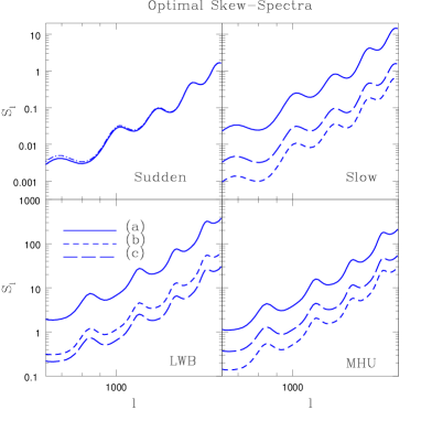
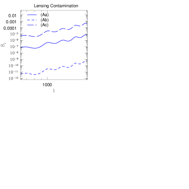
Figure 8: Left panel: optimum skew-spectrum, $S^{\Theta\rm E,X}_{\ell}$, defined in Eq.(22) for different reionization history models and tracer fields. The solid lines corresponds to model (a), short-dashed lines to model (b) and long-dashed lines to model (c). Right panel: lensing contamination to the optimum estimator evaluated using Eq. (30) in the case of the “slow” reionization history model, other scenarios have similar magnitudes.

Modelling of reionization history is important not only for astrophysical understanding of the process, but it is also crucial for accurate estimation of cosmological parameters, as inaccuracy can translate into strongly biased parameters. We have used the mixed bispectrum involving temperature, polarization and external tracers to map out the reionization history of the Universe.

Models and Tracers: We have used four different models of reionization (A) slow, (B) sudden, (C) LWB, (D) MHU to study non-Gaussianity induced by reionization. The ionization fraction corresponding to these scenarios are plotted in Fig. 2 (left-panel) and Fig. 2. The parametrization of the ionization fractions ${x}_{e}(r)$ is based on an average redshift of reionization $\bar{z}$ and a transition width $\sigma_{z}$. Note that we have applied our analysis not only to a single stage reionization, but also to more complicated scenarios involving multiple stages of reionization. For external tracer fields we include three different source populations: (a) proto-galaxy distribution, (b) 21cm-emitting neutral hydrogen sources, and (c) quasar distribution. We model the distribution of these sources with redshift (in 3D) using a simple parametric fit. The redshift dependence of these tracers is plotted in Fig. 2 (right-panel).

Estimators, Optimum and Sub-optimum: The cross-correlation of these 3D tracer fields with 2D temperature $\Theta$ and E-type polarization maps $E$ produces a 3D skew-spectrum $S_{\ell}(r)$ that is presented in Eq. (22). To construct the 3D skew-spectrum we construct the harmonics ${\cal A}_{\ell m}(r),{\cal B}_{\ell m}(r)$ and ${\cal C}_{\ell m}(r)$ from $\Theta_{\ell m}$, $E_{\ell m}$ and $S_{\ell m}$ with suitable weighting factors. The weights depends on the background cosmology and the spectrum of fields and relevant power-spectra ${\cal C}_{\ell}^{\Theta\rm E}$, ${\cal C}^{\rm EE}_{\ell}$ and ${\cal C}^{\Theta\rm S}_{\ell}$. The exact expressions are given in Eq. (20). The power spectra ${\cal C}_{\ell}^{\rm EE}$ and ${\cal C}_{\ell}^{\Theta E}$ are presented in Fig. 4. A line of sight integration is finally used to compute the projected 2D estimator $S_{\ell}$ from its 3D analogue $S_{\ell}(r)$. The other power spectra that are used are plotted in Fig. 4 and 4. The optimal estimator introduced in Eq.(19) generalize a direct PCL based estimator in Eq. (14). As shown in Eq.(15) depending on the indices that are summed over, we can in principle construct three different similar power-spectra. The three different estimators will carry complementary information and when collapsed to a one-point estimator (skewness) they can provide an important cross-check for systematics. In Eq. (22) we have used estimators that are optimal. Implementation of such estimator for inhomogeneous noise and partial sky coverage has already been worked out in detail and was adopted for analysis of data from Planck (Munshi & Heavens, 2010), mainly in search for primordial non-Gaussianity.

The results from the computation of the optimum skew-spectra $S^{\Theta\rm E,X}_{\ell}$ are presented in Fig. 8. The amplitude of the skew-spectrum correlates strongly with the redshift range covered by the tracers.

Scatter, Signal-to-Noise and Contamination: The signal-to-noise of detection for individual models are shown in Table LABEL:table:s2n. For some models it can actually reach $({\rm S/\rm N})\approx 70$ but typically remains at a level of $({\rm S/\rm N})\approx 20$, thus indicating that such measurements can distinguish among different reionization scenarios at high statistical significance. In Fig. 7 we present the optimal skew-spectra results for MHU and LWB models.

Table 2: The signal to noise $({\rm S/N})$ of the optimum skew-spectrum estimator for four different reionization scenarios up to $\ell_{\rm max}=2000$ (without detector noise) are shown for various tracer fields. In our estimation we assume all-sky coverage and PLANCK errors. In the top row, results for two different scenarios (A) and (B), which correspond to “slow” and “sudden” transitions are shown. The bottom row displays results for LWB and MHU reionization. The numbers in the parentheses correspond to the realistic values of $({\rm S/N})$ with Planck type noise and sky coverage $f_{\rm sky}=0.8$.

	a	b	c
A (slow)	68.6 (36.5)	14.5 (7.5)	23.0 (13.0)
B (sudden)	23.4 (12.6)	-	23.5 (13.2)
LWB	76.6 (39.0)	31.5 (15.8)	22.0 (12.2)
MHU	57.6 (29.1)	21.2 (10.5)	29.5 (15.7)

The main source of contamination to our estimator is from lensing of CMB. To compute the level of contamination we have used the “slow” model for various tracer fields. We find contamination to be several order of magnitude lower than the signal. For other models we expect similar result.

5 Conclusion

The free electron population during reionization epoch re-scatters the local CMB temperature quadrupole and generates an additional polarization signal at small angular (arcminutes) scale. Due to their small amplitude, this contribution cannot be studied using the CMB temperature-polarization cross-spectra. However, additional information regarding the temporal evolution of the spatial variation of the free electron density can be gained by studying the three-way correlation between temperature anisotropy, polarisation and an external field, which can act as a tracer field for the free electron density. In harmonic space the associated mixed bispectrum can be used to constrain models of reionization. Estimation of individual modes of bispectra are dominated by noise, so the majority of studies in the past have used the skewness, which compresses all available modes to a single high (S/N) number, but this may mask the reionization history. Here we have shown how the recently proposed skew-spectra can be used to discriminate between models of reionization. We find that the amplitude of the skew-spectra correlates strongly with the epoch of reionization as well as the redshift distribution of tracers. We have studied four different models of reionization and three realistic tracers. We find that the use of multiple tracers can be very powerful in probing the redshift evolution of the ionization fraction. Most of the signal comes from high $\ell$ hence surveys and tracers with limited sky coverage can also provide valuable information and all-sky coverage is not an absolute necessity. Our results correspond to a Planck-type beam but experiments with even higher angular resolution will be able to achieve higher (S/N). In principle with judicious choice of different tracers it will be possible to map out the entire ionization history.

We develop both the direct or PCL-based estimators as well as inverse covariance-weighted optimal estimators. For each choice of tracer field, we develop three set of estimators for cross-validation in Eq. (18). The contamination from weak-lensing was found to be negligible. In case of an ideal experiment without detector noise, depending on the redshift distribution of the tracer field, the (S/N) for detection of skew-spectra can reach relatively high values in most scenarios typically ${\cal O}(20)$, and even higher for some scenarios. For Planck type experiment the (S/N) for most scenarios is typically ${\cal O}(10)$.

In the text of the paper we have used the visibility function as our primary variable to describe the reionization history. In the Appendix we detail equivalent results for optical depth instead .The patchy reionization induces non-Gaussianity both due to patchy screening as well as Thomson scattering. We show that the estimators for reconstructing fluctuations in optical depth can be cross-correlated with external data sets, and the resulting estimators are similar to the skew-spectra but with different weights. These estimators that work with minimum variance reconstruction of optical depth are however are not optimal and differ from the corresponding PCL estimators. Cross-correlating with tracers which have redshift information has the advantage of distinguishing different histories of reionization. It is generally believed that the polarization from late-time reionization by patchy screening is small compared with polarization due to late-time Thomson scattering during reionization. However recent studies based on power-spectrum analysis have shown that at small angular scales both effects are comparable (Dvorkin, Hu & Smith, 2009). We derive the bispectrum generated by patchy screening of primary as well as by late-time Thomson scattering.

The primary motivation of this paper was to devise a method to distinguish between different reionization histories of the Universe, using non-Gaussianity induced by the fluctuations in optical depth. This has been achieved, using mixed bispectra of CMB temperature and polarisation fields, along with one or more foreground tracers of free electron density. Using skew-spectra, originally devised for studies of primordial non-Gaussianity, we find that different reionization history models can be distinguished with this method with high signal-to-noise.

We have assumed a perfect subtraction of all foregrounds to arrive at our results. Needless to say, that, as in any study using CMB data, unsubtracted residuals from the component separation step of the data reduction pipeline can seriously bias conclusion drawn using techniques presented here.

6 Acknowledgements

DM acknowledges support from the Science and Technology Facilities Council (grant numbers ST/L000652/1). We would like to thank Erminia Calabrese, Patrick Valageas, Asantha Cooray, Antony Lewis and Joseph Smidt for useful discussions. The Dark Cosmology Centre is funded by the Danish National Research Foundation. P.S.C. is supported by ERC Grant Agreement No. 279954.

Appendix A Bispectrum from patchy Reionization

In this appendix we show how the reconstruction of the optical depth $\tau$ and lensing potential $\phi$ studied in the literature (Dvorkin & Smith, 2009; Dvorkin, Hu & Smith, 2009; Meerburg, Dvorkin & Spergel, 2013) using quadratic potential is linked to our PCL estimator and the optimum estimator used in the text of the paper. We will consider contribution from patchy screening and lensing of the CMB. See e.g. Weller (1999); Liu et al. (2001); Dore et al. (2007) for various aspects of patchy reionization.

A.1 Patchy Reionization

Reionization can introduce screening of the temperature and polarization from the surface of last scattering (Dvorkin & Smith, 2009). Individual line of sight temperature and polarization gets multiplied by $e^{-\tau(\hat{\bf\Omega})}$ where $\tau$ is the optical depth towards the direction $\hat{\bf\Omega}$. In case of inhomogeneous reionization (IR) this effect is known to generate addition B-mode polarization (Dvorkin, Hu & Smith, 2009). In the text of the paper the visibility function $g(r)$ was treated primary variable. Equivalently, following Dvorkin & Smith (2009) the optical depth $\tau$ will be considered below as the primary variable instead. The optical depth to a radial comoving distance $r$ along the line of sight is given by:

$$\tau(\hat{\bf\Omega},z)=\sigma_{\rm T}n_{{\rm p},0}\int_{0}^{z}dz^{\prime}\;{(1+z^{\prime})^{2}\over H(z^{\prime})}\;x_{\rm e}(\hat{\bf\Omega},z^{\prime}).$$ (33)

Here $n_{{\rm p},0}$ is the number density of protons at redshift $z=0$ and $x_{\rm e}(\hat{\bf\Omega},z)$ is the ionization fraction.

$$p_{\pm}(\hat{\bf\Omega})=({q}\pm i{u})(\hat{\bf\Omega})=\int_{0}^{\infty}\,dr\,\dot{\tau}\,\exp[-\tau(\hat{\bf\Omega},r)]\,S^{\pm}_{\rm pol}(\hat{\bf\Omega},r);\quad\quad S^{\pm}_{\rm pol}(\hat{\bf\Omega},r)=-{\sqrt{24\pi}\over 10}\sum_{m=-2}^{2}{}_{\pm 2}Y_{2m}(\hat{\bf\Omega},r)\Theta_{2m}.$$ (34)

Writing $x_{\rm e}(\hat{\bf\Omega},r)$ as a sum of redshift dependent angular average $\bar{x}_{\rm e}(r)$ and a fluctuating term $\delta x_{\rm e}(\hat{\bf\Omega},r)$ i.e. $x_{\rm e}(\hat{\bf\Omega},r)=\bar{x}_{\rm e}(r)+\Delta x_{\rm e}(\hat{\bf\Omega},r)$. Expanding $p_{\pm}(\hat{\bf\Omega})$ in a functional Taylor series we can write:

$$p_{\pm}(\hat{\bf\Omega})=p_{\pm}^{(0)}(\hat{\bf\Omega})+\sigma_{\rm T}n_{e}\int{dr\over a^{2}}\Delta x_{\rm e}\;p^{(1)}_{\pm}(\hat{\bf\Omega},r).$$ (35)

The zeroth-order term $p_{\pm}^{(0)}(\hat{\bf\Omega})$ is the polarization from recombination and homogeneous reionization. The first-order correction $p_{\pm}^{(1)}(\hat{\bf\Omega})$ is due to inhomogeneous reionization:

$$p^{(1)}_{\pm}(\hat{\bf\Omega},r)=\int_{r}^{\infty}dr^{\prime}{\delta(P_{\pm}(\hat{\bf\Omega}))\over\delta\tau(r^{\prime})}=\left[e^{-\tau}S_{\pm}(\hat{\bf\Omega},r)-\int_{r}^{\infty}dr^{\prime}\dot{\tau}\;e^{-\tau}S(\hat{\bf\Omega},r^{\prime})\right].$$ (36)

The two terms correspond to screening and Thomson scattering respectively. For temperature and polarization we have:

$$p_{\pm}(\hat{\bf\Omega})=p_{\pm}^{(0)}(\hat{\bf\Omega})+\sum_{i}\delta\tau^{(i)}(\hat{\bf\Omega})\;[p^{(1)}_{\pm}(\hat{\bf\Omega})]^{(i)};\quad\quad\Theta(\hat{\bf\Omega})=\Theta_{0}(\hat{\bf\Omega})+\sum_{i}\delta\tau^{(i)}(\hat{\bf\Omega})\Theta^{(i)}_{1}(\hat{\bf\Omega}).$$ (37)

The discrete version of Eq.(36) that involves redshift binning can be introduced by restricting the integral in Eq.(33) into a particular redshift interval. The contributions from a particular tomographic bin is denoted as $\tau^{(i)}$, $\Theta^{(1)}$ and $[p^{(1)}_{\pm}]^{(i)}$. To define an estimator for $\tau$ we can write for arbitrary fields $\rm X$ and $\rm Y$:

$$\langle{\rm X}_{\ell_{1}m_{1}}{\rm Y}_{\ell_{2}m_{2}}\rangle=(-1)^{m_{2}}{\cal C}_{\ell_{1}}^{\rm XY}\delta_{\ell_{1}\ell_{2}}\delta_{m_{1}-m_{2}}+\sum_{\ell_{1}\ell_{2}}\Gamma^{\rm XY}_{\ell_{1}\ell_{2}\ell}\left(\begin{array}[]{ c c c }\ell_{1}&\ell_{2}&\ell\\ m_{1}&m_{2}&m\end{array}\right){\Delta\tau}_{\ell m};\quad({\rm X,Y})\in{\Theta,\rm E,B};$$ (40)

$$\hat{\tau}_{\ell m}={\rm N}_{\ell}\sum_{\ell_{1}m_{1}}\sum_{\ell_{2}m_{2}}\Gamma^{\rm XY}_{\ell_{1}\ell_{2}\ell}\left(\begin{array}[]{ c c c }\ell_{1}&\ell_{2}&\ell\\ m_{1}&m_{2}&m\end{array}\right){{\rm X}_{\ell_{1}m_{1}}\over{\cal C}^{\rm XX}_{\ell_{1}}}{{\rm Y}_{\ell_{2}m_{2}}\over{\cal C}^{\rm YY}_{\ell_{2}}}.$$ (43)

The power spectra ${\cal C}^{\rm XX}_{\ell}=\langle X_{\ell m}X^{*}_{\ell m}\rangle$ and ${\cal C}^{\rm YY}_{\ell}=\langle Y_{\ell m}Y^{*}_{\ell m}\rangle$ also include respective noise. The normalisation ${\rm N}_{\ell}$ is fixed by demanding that the estimator be unbiased. The mode coupling matrix $\Gamma$ for various choices of variables $\rm X$ and $\rm Y$ are listed below (Dvorkin & Smith, 2009):

$$\Gamma^{\rm\Theta\Theta}_{\ell_{1}\ell_{2}\ell}=\left[{\cal C}^{\rm\Theta_{0}\Theta_{1}}_{\ell_{1}}+{\cal C}_{\ell_{2}}^{\rm\Theta_{0}\Theta_{1}}\right]R^{000}_{\ell_{1}\ell_{2}\ell};$$ (44)

$$\Gamma^{\rm EE}_{\ell_{1}\ell_{2}\ell}=\left[{\cal C}^{\rm E_{0}E_{1}}_{\ell_{1}}+{\cal C}_{\ell_{2}}^{\rm E_{0}E_{1}}\right]\left[R^{-220}_{\ell_{1}\ell_{2}\ell}+R^{2-20}_{\ell_{1}\ell_{2}\ell}\right];$$ (45)

$$\Gamma^{\rm\Theta E}_{\ell_{1}\ell_{2}\ell}={{\cal C}_{\ell_{1}}^{\Theta_{0}E_{1}}\over 2}\left[R^{-220}_{\ell_{1}\ell_{2}\ell}+R^{2-20}_{\ell_{1}\ell_{2}\ell}\right]+{\cal C}^{\Theta_{1}E_{0}}_{\ell_{2}}R^{000}_{\ell_{1}\ell_{2}\ell};$$ (46)

$$\Gamma^{\rm\Theta B}_{\ell_{1}\ell_{2}\ell}={{\cal C}_{\ell_{1}}^{\Theta_{0}E_{1}}\over 2i}\left[R^{-220}_{\ell_{1}\ell_{2}\ell}-R^{2-20}_{\ell_{1}\ell_{2}\ell}\right]+{\cal C}^{T_{1}E_{0}}_{\ell_{2}}R^{000}_{\ell_{1}\ell_{2}\ell};$$ (47)

$$\Gamma^{\rm EB}_{\ell_{1}\ell_{2}\ell}={{\cal C}_{\ell_{1}}^{\Theta_{0}E_{1}}\over 2i}\left[R^{-220}_{\ell_{1}\ell_{2}\ell}-R^{2-20}_{\ell_{1}\ell_{2}\ell}\right];$$ (48)

$$R^{s_{1}s_{2}s_{3}}_{\ell_{1}\ell_{2}\ell}=\sqrt{\Sigma_{\ell_{1}}\Sigma_{\ell_{2}}\Sigma_{\ell_{3}}\over 4\pi}\left(\begin{array}[]{ c c c }\ell_{1}&\ell_{2}&\ell_{3}\\ s_{1}&s_{2}&s_{3}\end{array}\right).$$ (51)

In general a minimum variance estimator for $\tau$ can be obtained by including temperature and polarization maps and is expressed as:

$$\hat{\tau}_{\ell m}={{\rm N}_{\ell}\over 2}\sum_{\rm XY}\sum_{\rm X^{\prime}Y^{\prime}}\sum_{\ell_{1}m_{1}}\sum_{\ell_{2}m_{2}}\Gamma^{\rm XY}_{\ell_{1}\ell_{2}\ell}\left(\begin{array}[]{ c c c }\ell_{1}&\ell_{2}&\ell\\ m_{1}&m_{2}&m\end{array}\right)[C^{\rm XX^{\prime}}]^{-1}_{\ell_{1}m_{1}}{\rm X}^{\prime}_{\ell_{1}m_{1},\ell_{1}^{\prime}m_{1}^{\prime}}[C^{\rm YY^{\prime}}]^{-1}_{\ell_{2}m_{2},\ell_{2}^{\prime}m_{2}^{\prime}}{\rm Y}^{\prime}_{\ell_{2}^{\prime}m_{2}^{\prime}}.$$ (54)

We an cross-correlate the above minimum variance reconstruction of $\tau$ with an external tracer $\rm Z$ with redshift information:

$${\cal C}_{\ell}^{\tau\rm Z}={1\over 2\ell+1}\sum_{\ell_{1}\ell_{2}}\Gamma^{\rm XY}_{\ell_{1}\ell_{2}\ell}\;{B_{\ell_{1}\ell_{2}\ell}^{\rm XYZ}\over{\cal C}^{\rm XX}_{\ell_{1}}{\cal C}^{\rm YY}_{\ell_{2}}}.$$ (55)

The resulting estimator is sub-optimal and similar to our PCL defined in Eq.(14) and optimal estimator defined in Eq.(18). A specific model of reionization and its cross-correlation with an external tracer is required for explicit computation of ${\cal C}_{\ell}^{\tau\rm Z}$.

Some of the results presented here will be useful in probing reionization using the kinetic Sunyaev-Zeldovich effect (Park et al. (2013) and references therein).

A.2 Patchy Screening Induced non-Gaussianity and resulting non-Gaussianity

As discussed above, the scattering of CMB during reionization out of the line-of-sight suppresses the primary temperature polarization anisotropy from recombination as $\exp(-\tau)$ where $\tau$ is the Thomson optical depth. If $\tau$ varies across the line of sight this suppression itself induces anisotropy in temperature $\Theta(\hat{\bf\Omega})$ and polarization Stokes parameters. Following Dvorkin, Hu & Smith (2009) the amplitude modulation due to patchy screening an be expressed as:

$$\Theta(\hat{\bf\Omega})=\exp[-\tau(\hat{\bf\Omega})]\Theta^{(\rm rec)}(\hat{\bf\Omega});\quad\quad(\rm Q\pm iU)(\hat{\bf\Omega})=\exp[-\tau(\hat{\bf\Omega})](\rm Q\pm iU)^{(\rm rec)}(\hat{\bf\Omega})$$ (56)

where

$${\rm\Theta}^{(\rm rec)}(\hat{\bf\Omega})=\sum_{\ell m}\Theta^{\rm(rec)}_{\ell m}Y_{\ell m}(\hat{\bf\Omega});\quad\quad(\rm Q\pm i\rm U)^{(\rm rec)}(\hat{\bf\Omega})=-\sum_{\ell m}(E^{\rm(rec)}_{\ell m}\pm iB^{\rm(rec)}_{\ell m})[{}_{\pm 2}Y_{\ell m}(\hat{\bf\Omega})].$$ (57)

If we separate the monopole $\bar{\tau}$ and fluctuating component of the optical depth $\tau$, we can write $\tau(\hat{\bf\Omega})=\bar{\tau}+\sum_{\ell m}\tau_{\ell m}Y_{\ell m}(\hat{\bf\Omega})$. Assuming $\delta\tau\equiv(\tau(\hat{\bf\Omega})-\bar{\tau})\ll 1$ in the harmonic domain we have $\Theta_{\ell m}=\exp(-\bar{\tau})\Theta^{\rm rec}_{\ell m}+\Theta^{\rm scr}_{\ell m}$ and similarly for other harmonics $E_{\ell m}$ and $B_{\ell m}$. Here $\Theta^{\rm(rec)}$ is same as $\Theta^{(0)}$ of previous section. The screening contribution can be expressed as a function of fluctuation in $\tau$ and respective fields at recombination (Dvorkin, Hu & Smith, 2009):

$$\Theta_{\ell m}^{(\rm scr)}=-\exp(-\bar{\tau})\sum_{\ell^{\prime}m^{\prime}\ell^{\prime\prime}m^{\prime\prime}}\delta\tau_{\ell^{\prime\prime}m^{\prime\prime}}\Theta^{\rm(rec)}_{\ell^{\prime}m^{\prime}}\;R^{000}_{\ell\ell^{\prime}\ell^{\prime\prime}}\left(\begin{array}[]{ c c c }\ell&\ell^{\prime}&\ell^{\prime\prime}\\ m&m^{\prime}&m^{\prime\prime}\end{array}\right);$$ (60)

$$E_{\ell m}^{(\rm scr)}=-\exp(-\bar{\tau})\sum_{\ell^{\prime}m^{\prime}\ell^{\prime\prime}m^{\prime\prime}}\delta\tau_{\ell^{\prime\prime}m^{\prime\prime}}E^{(rec)}_{\ell^{\prime}m^{\prime}}\epsilon_{\ell\ell^{\prime}\ell^{\prime\prime}}\;R^{220}_{\ell\ell^{\prime}\ell^{\prime\prime}}\left(\begin{array}[]{ c c c }\ell&\ell^{\prime}&\ell^{\prime\prime}\\ m&m^{\prime}&m^{\prime\prime}\end{array}\right);$$ (63)

$$iB_{\ell m}^{(\rm scr)}=-\exp(-\bar{\tau})\sum_{\ell^{\prime}m^{\prime}\ell^{\prime\prime}m^{\prime\prime}}\delta\tau_{\ell^{\prime\prime}m^{\prime\prime}}E^{(rec)}_{\ell^{\prime}m^{\prime}}\beta_{\ell\ell^{\prime}\ell^{\prime\prime}}\;R^{220}_{\ell\ell^{\prime}\ell^{\prime\prime}}\left(\begin{array}[]{ c c c }\ell&\ell^{\prime}&\ell^{\prime\prime}\\ m&m^{\prime}&m^{\prime\prime}\end{array}\right);$$ (66)

$$\epsilon_{\ell\ell^{\prime}\ell^{\prime\prime}}={1\over 2}[1+(-1)^{\ell+\ell^{\prime}+\ell^{\prime\prime}}];\quad\beta_{\ell\ell^{\prime}\ell^{\prime\prime}}={1\over 2}[1-(-1)^{\ell+\ell^{\prime}+\ell^{\prime\prime}}].$$ (67)

The mixed bispectrum involving $\Theta_{\ell m}$, $E_{\ell m}$ and an external tracer field ${\rm X}_{\ell m}$ has a vanishing contribution at the leading order, if we assume vanishing cross-correlation between CMB fluctuations generated at recombination and the local tracer field. However, at next-to-leading order the bispectrum can be computed using a model for cross-spectra involving $\tau$ and $X$, denoted as ${\cal C}^{\tau X}_{\ell}$. The corresponding bispectrum takes the following form:

$$B^{\rm\Theta\bf EX}_{\ell\ell^{\prime}\ell^{\prime\prime}}=\exp(-2\bar{\tau}){\cal C}_{\ell^{\prime}}^{\rm\Theta E}{\cal C}_{\ell^{\prime\prime}}^{X\rm\tau}\left[\epsilon_{\ell\ell^{\prime}\ell^{\prime\prime}}W_{\ell\ell^{\prime}\ell^{\prime}}^{220}+W_{\ell\ell^{\prime}\ell^{\prime}}^{000}\right].$$ (68)

Corresponding results for other combinations of harmonics can be derived using similar reasoning. The related optimum skew-spectra can be constructed using these bispectra in Eq.(19). Similarly the resulting PCL skew-spectra can be constructed using Eq.(14).

Appendix B Lensing Reconstruction and Contamination

The reconstruction of the lensing potential of the CMB can be treated in an equivalent manner (Dvorkin & Smith, 2009). Minimum variance quadratic estimators in line with Eq.(54) can be constructed using the following coupling functions:

$$\Lambda^{\Theta\Theta}_{\ell_{1}\ell_{2}\ell}=\left[{\cal C}^{\Theta\Theta}_{\ell_{1}}F^{0}_{\ell_{2}\ell_{1}\ell}+{\cal C}_{\ell_{2}}^{\Theta\Theta}F^{0}_{\ell_{1}\ell_{2}\ell}\right];$$ (69)

$$\Lambda^{\Theta\rm E}_{\ell_{1}\ell_{2}\ell}={1\over 2}{\cal C}^{\Theta\rm E}_{\ell_{1}}\left[F^{-2}_{\ell_{2}\ell_{1}\ell}+F^{2}_{\ell_{2}\ell_{1}\ell}\right]+{\cal C}^{\Theta\rm E}_{\ell_{2}}F^{0}_{\ell_{1}\ell_{2}\ell}\;\;;$$ (70)

$$\Lambda^{\rm EE}_{\ell_{1}\ell_{2}\ell}={{\cal C}_{\ell_{1}}^{\rm EE}\over 2}\left[F^{-2}_{\ell_{2}\ell_{1}\ell}+F^{2}_{\ell_{2}\ell_{1}\ell}\right]+{{\cal C}^{\rm EE}_{\ell_{2}}\over 2}\left[F^{-2}_{\ell_{1}\ell_{2}\ell}+F^{2}_{\ell_{1}\ell_{2}\ell}\right];$$ (71)

$$\Lambda^{\Theta\rm E}_{\ell_{1}\ell_{2}\ell}={{\cal C}_{\ell_{1}}^{\Theta\rm E}\over 2i}\left[F^{-2}_{\ell_{2}\ell_{1}\ell_{3}}-F^{2}_{\ell_{2}\ell_{1}\ell}\right];$$ (72)

$$\Lambda^{\rm EB}_{\ell_{1}\ell_{2}\ell}={{\cal C}_{\ell_{1}}^{\Theta\rm E}\over 2i}\left[F^{-2}_{\ell_{2}\ell_{1}\ell_{3}}-F^{2}_{\ell_{2}\ell_{1}\ell}\right];$$ (73)

$$F^{\pm s}_{\ell_{1}\ell_{2}\ell}=\sqrt{\Sigma_{\ell_{1}}\Sigma_{\ell_{2}}\Sigma_{\ell_{3}}\over 4\pi}\left[-\Pi_{\ell_{1}}+\Pi_{\ell_{2}}+\Pi_{\ell_{3}}\right]\left(\begin{array}[]{ c c c }\ell_{1}&\ell_{2}&\ell_{3}\\ \mp s&\pm s&0\end{array}\right).$$ (76)

Using these expressions for $\Lambda^{\rm XY}_{\ell_{1}\ell_{2}\ell}$ in Eq.(69)-Eq.(76) we can construct an estimator for the lensing potential $\phi$ in line with Eq.(54).

$$\hat{\phi}_{\ell m}={\rm N}_{\ell}\sum_{\ell_{1}m_{1}}\sum_{\ell_{2}m_{2}}\Lambda^{\rm XY}_{\ell_{1}\ell_{2}\ell}\left(\begin{array}[]{ c c c }\ell_{1}&\ell_{2}&\ell\\ m_{1}&m_{2}&m\end{array}\right){{\rm X}_{\ell_{1}m_{1}}\over{\cal C}^{\rm XX}_{\ell_{1}}}{{\rm Y}_{\ell_{2}m_{2}}\over{\cal C}^{\rm YY}_{\ell_{2}}}.$$ (79)

The corresponding estimator for the lensing skew-spectrum ${\cal C}^{\phi\rm Z}_{\ell}$ is

$${\cal C}_{\ell}^{\phi\rm Z}={1\over 2\ell+1}\sum_{\ell_{1}\ell_{2}}\Lambda^{\rm XY}_{\ell_{1}\ell_{2}\ell}\;{B_{\ell_{1}\ell_{2}\ell}^{\rm XYZ}\over{\cal C}^{\rm XX}_{\ell_{1}}{\cal C}^{\rm YY}_{\ell_{2}}}.$$ (80)

We considered the possibility of cross-correlating external tracers, but it is also possible to construct ${\cal C}^{\tau\tau}_{\ell}$ or ${\cal C}^{\phi\phi}_{\ell}$ for internal detection using CMB data alone, using the four-point correlation function or equivalently the trispectrum in the harmonic domain.

References

- Adshead & Furlanetto (2007) Adshead P., Furlanetto S., 2008, MNRAS, 384, 291
- Alvarez et al. (2006) Alvarez M.A., Komatsu E., Dore O., Shapiro P.R., 2006, Astrophys. J. 647, 840
- Barkana & Loeb (2001) Barkana R., Loeb A., 2001, Phys. Rept., 340, 291
- Bartolo et al. (2004) Bartolo N., Komatsu E., Matarrese S., Riotto A., 2004, Phys. Rept., 402, 103
- Bennett et al. (2013) Bennett C.L., 2013, ApJS, 208, 20
- Chen & Kamionkowski (2004) Chen X., Kamionkowski M., 2004, PRD, 70, 043502
- Cooray (2001) Cooray A., 2001, PRD, 64, 043516
- Cooray (2004) Cooray A., 2004, PRD, 70, 023508
- Creminelli et al. (2006) Creminelli P., Nicolis A., Senatore L., Tegmark M., Zaldarriaga M., 2006, JCAP, 03(05)004
- Creminelli, Senatore, & Zaldarriaga (2007) Creminelli P., Senatore L., Zaldarriaga M., 2007, JCAP, 03(07)019
- Dore et al. (2007) Doré O, Holder G., Alvarez M., Iliev I.T., Mellema G, Pen U-L., Shapiro P.R., 2007, PRD, 76, 043002
- Dvorkin & Smith (2009) Dvorkin C. Smith K. M., 2009, PRD, 79, 043003
- Dvorkin, Hu & Smith (2009) Dvorkin C, Hu W., Smith K.M., 2009, PRD, 79, 107302
- Edmonds (1968) Edmonds, A.R., Angular Momentum in Quantum Mechanics, 2nd ed. rev. printing. Princeton, NJ:Princeton University Press, 1968.
- Eisenstein & Hu (1998) Eisenstein D.J., Hu W., 1998, Astrophys. J., 496, 605
- Fan et al. (2006) Fan X.-H., Strauss M.A., Becker R.H., White R.L., Gunn J.E., et al., 2006 Astron. J., 132, 117
- Fax, Carli & Keating (2006) Fan X.-H., Carili C., Keating B.G., 2006, Ann. Rev. Astron. & Astrophysics, 44, 415
- Hansen & Haiman (2004) Hansen S.H., Haiman Z., 2004, Astrophys. J., 600, 26
- Heavens (1998) Heavens A.F., 1998, MNRAS, 299, 805
- Holder et al. (2008) Holder G., Haiman Z., Kaplinghat M., Knox L., 2003, Astrophys. J., 595, 13
- Holder, Iliev & Mellama (2007) Holder G., Iliev I.T., Mellema G., 2007, ApJL, 663, 1
- Hu (2008) Hu W., 2000, Astrophys. J., 529, 12
- Hu & Holder (2008) Hu W., Holder G.P., 2003, PRD, 68, 023001
- Kaplinghat et al. (2003) Kaplinghat M., Chu M., Haiman Z., Holder G., Knox L., Skordis C., 2003, ApJ. 583, 24
- Kasuya, Kawasaki & Sugiyama (2004) Kasuya S., Kawasaki M., Sugiyama N., 2004, PRD, 69, 023512
- Komatsu, Spergel & Wandelt (2005) Komatsu E., Spergel D. N., Wandelt B. D., 2005, Astrophys. J., 634, 14
- Khatri & Wandelt (2010) Khatri R., Wandelt B.D., 2009, PRD, 79, 3501
- Lewis, Weller & Battye (2006) Lewis A., Weller J., Battye R., 2006, MNRAS, 373, 561
- Liu et al. (2001) Liu G.-C., Sugiyama N., Benson A.J., Lacey C.G., Nusser A., 2001, Astrophys. J., 561, 504
- Loeb & Barkana (2001) Loeb A., Barkana R., 2001, Ann. Rev. Astron. & Astrophysics, 39, 19
- Meerburg, Dvorkin & Spergel (2013) Meerburg P.D., Dvorkin C., Spergel D.N., 2013, Astrophys. J., 779, 124
- Mortonson & Hu (2008) Mortonson M.J., Hu W., 2008, Astrophys. J., 672, 737
- Munshi & Heavens (2010) Munshi D., Heavens A., 2010, MNRAS, 401, 2406
- Munshi et al. (2011) Munshi D., Cooray A., Heavens A., Valageas P., 2011, MNRAS, 414, 3173
- Munshi et al. (2013b) Munshi D., Smidt J., Cooray A., Renzi A., Heavens A., Coles P., 2013, MNRAS, 434, 2830
- Munshi, Coles & Heavens (2013a) Munshi D., Coles P., Heavens A., 2013, MNRAS, 428, 2628
- Munshi et al. (2012a) Munshi D., Smidt J., Joudaki S., Coles P., 2012a, MNRAS, 419, 138.
- Munshi et al. (2012b) Munshi D., Smidt J., van Waerbeke L., Coles P., 2012b, MNRAS, 419, 536.
- Oh (2001) Oh S.P., 2001, Astrophys. J., 553, 4990
- Pandolfi et al. (2010) Pandolfi S., Cooray A., Giusarma E., Kolb E.W., Melchiorri A., Mena O., Serra P., 2010a, PRD, 81, 123509
- Pandolfi et al. (2010a) Pandolfi S., Giusarma E., Kolb E.W., Lattanzi M., Melchiorri A., Mena O., Pena M., Cooray A., Serra P., 2010b, PRD, 82, 123527
- Pandolfi et al. (2011) Pandolfi S., Ferrara A., Choudhury T. Roy, Melchiorri A., Mitra S., 2011c, PRD, 84, 3522
- Park et al. (2013) Park H., Shapiro P.R., Komatsu E., Iliev I.T., Ahn K., Mellema G., 2013, Astrophys. J, 769, 93
- Planck Collaboration (2013d) Planck Collaboration, 2013d, arXiv:1303.5076
- Planck Collaboration (2013a) Planck Collaboration, 2013a, arXiv:1303.5077
- Planck Collaboration (2013b) Planck Collaboration, 2013b, arXiv:1303.5084
- Planck Collaboration (2013c) Planck Collaboration, 2013c, arXiv:1303.5082
- Santos et al. (2003) Santos M.G., Cooray A., Haiman Z., Knox L., Ma C. P., 2003, ApJ., 598, 756
- Smith, Zahn & Dore (2000) Smith K.M., Zahn O., Dore O., 2007, Phys. Rev. D76:043510
- Smith & Zaldarriaga (2006) Smith K. M., Zaldarriaga M., 2006, arXiv:astro-ph/0612571
- Tashiro et al. (2010) Tashiro H., Aghanim N., Langer M., Douspis M., Zaroubi S., et al., 2010, MNRAS, 402, 2617
- Weller (1999) Weller J., Astrophys. J., 1999, 527, L1
- Yadav & Wandelt (2008) Yadav A. P. S., Wandelt B. D., 2008, PRL, 100, 181301