Density matrix minimization with $\ell_{1}$ regularization

Abstract.

We propose a convex variational principle to find sparse representation of low-lying eigenspace of symmetric matrices. In the context of electronic structure calculation, this corresponds to a sparse density matrix minimization algorithm with $\ell_{1}$ regularization. The minimization problem can be efficiently solved by a split Bergman iteration type algorithm. We further prove that from any initial condition, the algorithm converges to a minimizer of the variational principle.

1. Introduction

The low-lying eigenspace of operators has many important applications, including those in quantum chemistry, numerical PDEs, and statistics. Given a $n\times n$ symmetric matrix $H$, and denote its eigenvectors as $\{\Phi_{i}\},i=1,\ldots,n$. The low-lying eigenspace is given by the span of the first $N$ (usually $N\ll n$) eigenvectors.

In many scenario, the real interest is the subspace itself, but not a particular set of basis functions. In particular, we are interested in a sparse representation of the eigenspace. The eigenvectors form a natural basis set, but for oftentimes they are not sparse or localized (consider for example the eigenfunctions of the free Laplacian operator $-\Delta$ on a periodic box). This suggests asking for an alternative sparse representation of the eigenspace.

In quantum chemistry, the low-lying eigenspace for a Hamiltonian operator corresponds to the physically occupied space of electrons. In this context, a localized class of basis functions of the low-lying eigenspaces is called Wannier functions [Wannier:1937, Kohn:1959Wannier]. These functions provide transparent interpretation and understandings of covalent bonds, polarizations, etc. of the electronic structure. These localized representations are also the starting point and the essence for many efficient algorithms for electronic structure calculations (see e.g. the review article [Goedecker:99]).

1.1. Our contribution

In this work, we propose a convex minimization principle for finding a sparse representation of the low-lying eigenspace.

(1) $$\min_{P\in\mathbb{R}^{n\times n}}\operatorname{tr}(HP)+\frac{1}{\mu}\lVert P\rVert_{1}$$

$$\text{s.t.}\ P=P^{\mathrm{T}},\,\operatorname{tr}P=N,\,0\preceq P\preceq I,$$

where $\lVert\cdot\rVert_{1}$ is the entrywise $\ell_{1}$ matrix norm, $A\preceq B$ denotes that $B-A$ is a positive semi-definite matrix, and $\mu$ is a penalty parameter for entrywise sparsity. Here $H$ is an $n\times n$ symmetric matrix, which is the (discrete) Hamiltonian in the electronic structure context. The variational principle gives $P$ as a sparse representation of the projection operator onto the low-lying eigenspace.

The key observation here is to use the matrix $P$ instead of the wave functions $\Psi$. This leads to a convex variational principle. Physically, this corresponds to looking for a sparse representation of the density matrix. We also noted that in cases where we expect degeneracy or near-degeneracy of eigenvalues of the matrix $H$, the formulation in terms of the density matrix $P$ is more natural, as it allows fractional occupation of states. This is a further advantage besides the convexity.

Moreover, we design an efficient minimization algorithm based on split Bregman iteration to solve the above variational problem. Starting from any initial condition, the algorithm always converges to a minimizer.

1.2. Previous works

There is an enormous literature on numerical algorithms for Wannier functions and more generally sparse representation of low-lying eigenspace. The influential work [Marzari:1997] proposed a minimization strategy within the occupied space to find spatially localized Wannier functions (coined as “maximally localized Wannier functions”).

In [E:2010PNAS], the second author with his collaborators developed a localized subspace iteration (LSI) algorithm to find Wannier functions. The idea behind the LSI algorithm is to combine the localization step with the subspace iteration method as an iterative algorithm to find Wannier functions of an operator. The method has been applied to electronic structure calculation in [Garcia-CerveraLuXuanE:09]. As [Garcia-CerveraLuXuanE:09] shows, due to the truncation step involved, the LSI algorithm does not in general guarantee convergence.

As a more recent work in [OzolinsLaiCaflischOsher:13], $L_{1}$ regularization is proposed to be used in the variational formulation of the Schrödinger equation of quantum mechanics for creating compressed modes, a set of spatially localized functions $\{\psi_{i}\}_{i=1}^{N}$ in $\mathbb{R}^{d}$ with compact support.

(2) $$E=\min_{\Psi_{N}}\sum_{j=1}^{N}\left(\frac{1}{\mu}\left|\psi_{j}\right|_{1}+\langle\psi_{j},\hat{H}\psi_{j}\rangle\right)\quad\mbox{\text{s.t.}}\quad\langle\psi_{j},\psi_{k}\rangle=\delta_{jk},$$

where $\hat{H}=-\frac{1}{2}\Delta+V(\mathrm{x})$ is the Hamilton operator corresponding to potential $V(\mathrm{x})$, and the $L_{1}$ norm is defined as $\left|\psi_{j}\right|_{1}=\int|\psi_{j}|d\mathrm{x}$. This $L_{1}$ regularized variational approach describes a general formalism for obtaining localized (in fact, compactly supported) solutions to a class of mathematical physics PDEs, which can be recast as variational optimization problems. Although an efficient algorithm based on a method of splitting orthogonality constraints (SOC) [Lai:2014splitting] is designed to solve the above non-convex problem, it is still a big challenge to theoretically analyze the convergence of the proposed the algorithm.

The key idea in the proposed convex formulation (1) of the variational principle is the use of the density matrix $P$. The density matrix is widely used in electronic structure calculations, for example the density matrix minimization algorithm [LiNunesVanderbilt:93]. In this type of algorithm, sparsity of density matrix is specified explicitly by restricting the matrix to be a banded matrix. The resulting minimization problem is then non-convex and found to suffer from many local minimizers. Other electronic structure algorithms that use density matrix include density matrix purification [McWeeny:60], Fermi operator expansion algorithm [BaroniGiannozzi:92], just to name a few.

From a mathematical point of view, the use of density matrix can be viewed as similar to the idea of lifting, which has been recently used in recovery problems [CandesStrohmerVoroninski:13]. While a nuclear norm is used in PhaseLift method [CandesStrohmerVoroninski:13] to enhance sparsity in terms of matrix rank; we will use an entrywise $\ell_{1}$ norm to favor sparsity in matrix entries.

The rest of the paper is organized as follows. We formulate and explain the convex variational principle for finding localized representations of the low-lying eigenspace in Section 2. An efficient algorithm is proposed in Section 3 to solve the variational principle, with numerical examples presented in Section 4. The convergence proof of the algorithm is given in Section 5.

2. Formulation

Let us denote by $H$ a symmetric matrix coming from, for example, the discretization of an effective Hamiltonian operator in electronic structure theory. We are interested in a sparse representation of the eigenspace corresponding to its low-lying eigenvalues. In physical applications, this corresponds to the occupied space of a Hamiltonian; in data analysis, this corresponds to the principal components (for which we take the negative of the matrix so that the largest eigenvalue becomes the smallest). We are mainly interested in physics application here, and henceforth, we will mainly interpret the formulation and algorithms from a physical view point.

The Wannier functions, originally defined for periodic Schrödinger operators, are spatially localized basis functions of the occupied space. In [OzolinsLaiCaflischOsher:13], it was proposed to find the spatially localized functions by minimizing the variational problem

(3) $$\min_{\Psi\in\mathbb{R}^{n\times N},\,\Psi^{\mathrm{T}}\Psi=I}\operatorname{tr}(\Psi^{\mathrm{T}}H\Psi)+\frac{1}{\mu}\lVert\Psi\rVert_{1}$$

where $\lVert\Psi\rVert_{1}$ denotes the entrywise $\ell_{1}$ norm of $\Psi$. Here $N$ is the number of Wannier functions and $n$ is the number of spatial degree of freedom (e.g. number of spatial grid points or basis functions).

The idea of the above minimization can be easily understood by looking at each term in the energy functional. The $\operatorname{tr}(\Psi^{\mathrm{T}}H\Psi)$ is the sum of the Ritz value in the space spanned by the columns of $\Psi$. Hence, without the $\ell_{1}$ penalty term, the minimization

(4) $$\min_{\Psi\in\mathbb{R}^{n\times N},\,\Psi^{\mathrm{T}}\Psi=I}\operatorname{tr}(\Psi^{\mathrm{T}}H\Psi)$$

gives the eigenspace corresponds to the first $N$ eigenvalues (here and below, we assume the non-degeneracy that the $N$-th and $(N+1)$-th eigenvalues of $H$ are different). While the $\ell_{1}$ penalty prefers $\Psi$ to be a set of sparse vectors. The competition of the two terms gives a sparse representation of a subspace that is close to the eigenspace.

Due to the orthonormality constraint $\Psi^{\mathrm{T}}\Psi=I$, the minimization problem (3) is not convex, which may result in troubles in finding the minimizer of the above minimization problem and also makes the proof of convergence difficult.

Here we take an alternative viewpoint, which gives a convex optimization problem. The key idea is instead of $\Psi$, we consider $P=\Psi\Psi^{\mathrm{T}}\in\mathbb{R}^{n\times n}$. Since the columns of $\Psi$ form an orthonormal set of vectors, $P$ is the projection operator onto the space spanned by $\Psi$. In physical terms, if $\Psi$ are the eigenfunctions of $H$, $P$ is then the density matrix which corresponds to the Hamiltonian operator. For insulating systems, it is known that the off-diagonal terms in the density matrix decay exponentially fast [Kohn:59, Panati:07, Cloizeaux:64a, Cloizeaux:64b, Nenciu:83, Kivelson:82, NenciuNenciu:98, ELu:CPAM, ELu:13].

We propose to look for a sparse approximation of the exact density matrix by solving the minimization problem proposed in (1). The variational problem (1) is a convex relaxation of the non-convex variational problem

(5) $$\min_{P\in\mathbb{R}^{n\times n}}\operatorname{tr}(HP)+\frac{1}{\mu}\lVert P\rVert_{1}$$

$$\text{s.t.}\ P=P^{\mathrm{T}},\,\operatorname{tr}P=N,\,P=P^{2},$$

where the constraint $0\preceq P\preceq I$ is replaced by the idempotency constraint of $P$: $P=P^{2}$. The variational principle (5) can be understood as a reformulation of (3) using the density matrix as variable. The idempotency condition $P=P^{2}$ is indeed the analog of the orthogonality constraint $\Psi^{\mathrm{T}}\Psi=I$. Note that $0\preceq P\preceq I$ requires that the eigenvalues of $P$ (the occupation number in physical terms) are between $0$ and $1$, while $P=P^{2}$ requires the eigenvalues are either $0$ or $1$. Hence, the set

(6) $$\mathcal{C}=\{P:P=P^{\mathrm{T}},\,\operatorname{tr}P=N,\,0\preceq P\preceq I\}$$

is the convex hull of the set

(7) $$\mathcal{D}=\{P:P=P^{\mathrm{T}},\,\operatorname{tr}P=N,\,P=P^{2}\}.$$

Therefore (1) is indeed a convex relaxation of (5).

Without the $\ell_{1}$ regularization, the variational problems (1) and (5) become

(8) $$\min_{P\in\mathbb{R}^{n\times n}}\operatorname{tr}(HP)$$

$$\text{s.t.}\ P=P^{\mathrm{T}},\,\operatorname{tr}P=N,\,0\preceq P\preceq I,$$

and

(9) $$\min_{P\in\mathbb{R}^{n\times n}}\operatorname{tr}(HP)$$

$$\text{s.t.}\ P=P^{\mathrm{T}},\,\operatorname{tr}P=N,\,P=P^{2}.$$

These two minimizations actually lead to the same result in the non-degenerate case.

Proposition 1.

Let $H$ be a symmetric $n\times n$ matrix. Assume that the $N$-th and $(N+1)$-th eigenvalues of $H$ are distinct, the minimizers of (8) and (9) are the same.

This is perhaps a folklore result in linear algebra, nevertheless we include the short proof here for completeness.

Proof.

It is clear that the unique minimizer of (9) is given by the projection matrix on the first $N$ eigenvectors of $H$, given by

$$P_{N}=\sum_{i=1}^{N}v_{i}v_{i}^{\mathrm{T}}$$

where $\{v_{i}\},i=1,\ldots,n$ are the eigenvectors of $H$, ordered according to their associated eigenvalues. Let us prove that (8) is minimized by the same solution.

Assume $P$ is a minimizer of (8), we calculate

(10) $$\operatorname{tr}(HP)=\sum_{i=1}^{n}v_{i}^{\mathrm{T}}HPv_{i}=\sum_{i=1}^{n}\lambda_{i}v_{i}^{\mathrm{T}}Pv_{i}=\sum_{i=1}^{n}\lambda_{i}\theta_{i}(P),$$

where $\theta_{i}(P)=v_{i}^{\mathrm{T}}Pv_{i}$. On the other hand, we have

$$\operatorname{tr}(P)=\sum_{i=1}^{n}v_{i}^{\mathrm{T}}Pv_{i}=\sum_{i=1}^{n}\theta_{i}(P)=N,$$

and $0\leq\theta_{i}(P)\leq 1$ since $0\preceq P\preceq I$. Therefore, if we view (10) as a variational problem with respect to $\{\theta_{i}\}$, it is clear that the unique minimum is achieved when

$$\theta_{i}(P)=\begin{cases}1,&i\leq N;\\ 0,&\text{otherwise}.\end{cases}$$

We conclude the proof by noticing that the above holds if and only if $P=P_{N}$. ∎

This result states that we can convexify the set of admissible matrices. We remark that, somewhat surprisingly, this result also holds for the Hartree-Fock theory [Lieb:77] which can be vaguely understood as a nonlinear eigenvalue problem. However the resulting variational problem is still non-convex for the Hartree-Fock theory.

Proposition 1 implies that the variational principle (1) can be understood as an $\ell_{1}$ regularized version of the variational problem (9). The equivalence no longer holds for (1) and (5) with the $\ell_{1}$ regularization. The advantage of (1) over (5) is that the former is a convex problem while the latter is not.

Coming back to the properties of the variational problem (1). We note that while the objective function of (1) is convex, it is not strictly convex as the $\ell_{1}$-norm is not strictly convex and the trace term is linear. Therefore, in general, the minimizer of (1) is not unique.

Example 1.

Let $\mu\in\mathbb{R}_{+}$, $N=1$ and

(11) $$H=\begin{pmatrix}1&0\\ 0&1\end{pmatrix},$$

The non-uniqueness comes from the degeneracy of the Hamiltonian eigenvalues. Any diagonal matrix $P$ with trace $1$ and non-negative diagonal entries is a minimizer.

Example 2.

Let $\mu=1$, $N=1$ and

(12) $$H=\begin{pmatrix}1&0&0\\ 0&2&2\\ 0&2&2\end{pmatrix}$$

The non-uniqueness comes from the competition between the trace term and the $\ell_{1}$ regularization. The eigenvalues of $H$ are $0,1$ and $4$. Straightforward calculation shows that

(13) $$P_{0}=\begin{pmatrix}0&0&0\\ 0&1/2&-1/2\\ 0&-1/2&1/2\end{pmatrix}$$

which corresponds to the eigenvector $(0,\sqrt{2}/2,-\sqrt{2}/2)^{\mathrm{T}}$ associated with eigenvalue $0$ and

(14) $$P_{1}=\begin{pmatrix}1&0&0\\ 0&0&0\\ 0&0&0\end{pmatrix}$$

which corresponds to the eigenvector $(1,0,0)^{\mathrm{T}}$ associated with eigenvalue $1$ are both minimizers of the objective function $\operatorname{tr}(HP)+\lVert P\rVert_{1}$. Actually, due to convexity, any convex combination of $P_{0}$ and $P_{1}$ is a minimizer too.

It is an open problem under what assumptions that the uniqueness is guaranteed.

3. Algorithm

To solve the proposed minimization problem (1), we design a fast algorithm based on split Bregman iteration [Goldstein:2009split], which comes from the ideas of variables splitting and Bregman iteration [Osher:2005]. Bregman iteration has attained intensive attention due to its efficiency in many $\ell_{1}$ related constrained optimization problems [Yin:2008bregman, yin2013error]. With the help of auxiliary variables, split Bregman iteration iteratively approaches the original optimization problem by computation of several easy-to-solve subproblems. This algorithm popularizes the idea of using operator/variable splitting to solve optimization problems arising from information science. The equivalence of the split Bregman iteration to the alternating direction method of multipliers (ADMM), Douglas-Rachford splitting and augmented Lagrangian method can be found in [Esser:2009CAM, Setzer:2009SSVMCV, Wu:2010SIAM].

By introducing auxiliary variables $Q=P$ and $R=P$, the optimization problem (1) is equivalent to

(15) $$\min_{P,Q,R\in\mathbb{R}^{n\times n}}\frac{1}{\mu}\lVert Q\rVert_{1}+\operatorname{tr}(HP)$$

$$\text{s.t.}\ Q=P,\,R=P,\,\operatorname{tr}P=N,\,R=R^{\mathrm{T}},\,0\preceq R\preceq I,$$

which can be iteratively solved by:

(16) $$(P^{k},Q^{k},R^{k}) =\arg\min_{P,Q,R\in\mathbb{R}^{n\times n}}\frac{1}{\mu}\lVert Q\rVert_{1}+\operatorname{tr}(HP)+\frac{\lambda}{2}\|P-Q+b\|_{F}^{2}+\frac{r}{2}\|P-R+d\|^{2}_{F}$$

$$\qquad\text{s.t.}\qquad\operatorname{tr}P=N,\,R=R^{\mathrm{T}},\,0\preceq R\preceq I,$$

(17) $$b^{k} =b^{k-1}+P^{k}-Q^{k}$$

(18) $$d^{k} =d^{k-1}+P^{k}-R^{k}$$

where variables $b,d$ are essentially Lagrangian multipliers and parameters $r,\lambda$ control the penalty terms. Solving $P^{k},Q^{k},R^{k}$ in (3) alternatively, we have the following algorithm.

Algorithm 2.

Initialize $Q^{0}=R^{0}=P^{0}\in\mathcal{C},b^{0}=d^{0}=0$

while “not converge” do

      

1. $\displaystyle P^{k}=\arg\min_{P\in\mathbb{R}^{n\times n}}\operatorname{tr}(HP)+\frac{\lambda}{2}\|P-Q^{k-1}+b^{k-1}\|_{F}^{2}+\frac{r}{2}\|P-R^{k-1}+d^{k-1}\|^{2}_{F},~{}\text{s.t.}~{}\operatorname{tr}P=N$.

2. $\displaystyle Q^{k}=\arg\min_{Q\in\mathbb{R}^{n\times n}}\frac{1}{\mu}\lVert Q\rVert_{1}+\frac{\lambda}{2}\|P^{k}-Q+b^{k-1}\|_{F}^{2}$.

3. $R^{k}=\displaystyle\arg\min_{R\in\mathbb{R}^{n\times n}}\frac{r}{2}\|P^{k}-R+d^{k-1}\|^{2}_{F},\quad\text{s.t.}\quad R=R^{\mathrm{T}},\,0\preceq R\preceq I$.

4. $b^{k}=b^{k-1}+P^{k}-Q^{k}$.

5. $d^{k}=d^{k-1}+P^{k}-R^{k}$.

Note that the minimization problem in the steps of Algorithm 2 can be solved explicitly, as follows:

(19) $$P^{k} =B^{k}-\frac{\operatorname{tr}(B^{k})-N}{n},$$

$$\quad\text{where }\quad B^{k}=\frac{\lambda}{\lambda+r}(Q^{k-1}-b^{k-1})+\frac{r}{\lambda+r}(R^{k-1}-d^{k-1})-\frac{1}{\lambda+r}H$$

(20) $$Q^{k} =\operatorname{Shrink}\left(P^{k}+b^{k-1},\frac{1}{\lambda\mu}\right)=\operatorname{sign}(P^{k}+b^{k-1})\max\left\{|P^{k}+b^{k-1}|-\frac{1}{\lambda\mu},0\right\}$$

(21) $$R^{k} =V\min\{\max\{D,0\},1\}V^{T},\text{ where }[V,~{}D]=\operatorname{eig}(P^{k}+d^{k-1}).$$

Starting form any initial guess, the following theorem guarantees that the algorithm converges to one of the minimizers of the variational problem (15).

Theorem 3.

The sequence $\big{\{}(P^{k},Q^{k},R^{k})\big{\}}_{k}$ generated by Algorithm 2 from any starting point converges to a minimum of the variational problem (15).

We will prove a slightly more general version of the above (Theorem 6). The idea of the proof follows from the general framework of analyzing split Bregman iteration, i.e. alternating direction method of multipliers (ADDM), see for example [GlowinskiLeTallec:89]. The standard proof needs to be generalized to cover the current case of “two level splitting” and the non-strictly convexity of the functionals. We defer the detailed proof to Section 5.

4. Numerical results

In this section, numerical experiments are presented to demonstrate the proposed model (1) for density matrix computation using algorithm 2. We illustrate our numerical results in three representative cases, free electron model, Hamiltonian with energy band gap and a non-uniqueness example of the proposed optimization problem. All numerical experiments are implemented by MATLAB in a PC with a 16G RAM and a 2.7 GHz CPU.

4.1. 1D Laplacian

In the first example, we consider the proposed model for the free electron case, in other words, we consider the potential free Schrödinger operator $-1/2\Delta$ defined on 1D domain $\Omega=[0,~{}100]$ with periodic boundary condition. This model approximates the behavior of valence electrons in a metallic solid with weak atomic pseudopotentials. In this case, the matrix $H$ is a central difference discretization of $-1/2\Delta$ on $[0,~{}100]$ with equally spaced $256$ points, and we take $N=10$. Figure 1(a) illustrates the true density matrix $\sum_{i=1}^{10}|\phi_{i}\rangle\langle\phi_{i}|$ obtained by the first $10$ eigenfunctions of $H$. As the free Laplacian does not have a spectral gap, the density matrix decays slowly in the off-diagonal direction. Figure 1(b) and (c) plot the density matrices obtained from the proposed model with parameter $\mu=10$ and $100$. Note that they are much localized than the original density matrix. As $\mu$ gets larger, the variational problem imposes a smaller penalty on the sparsity, and hence the solution for $\mu=100$ has a wider spread than that for $\mu=10$.

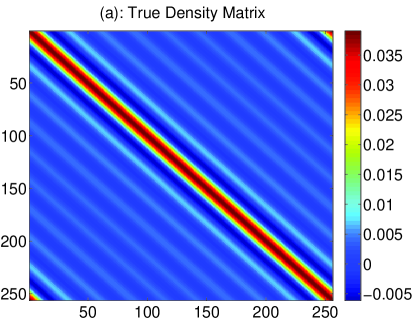
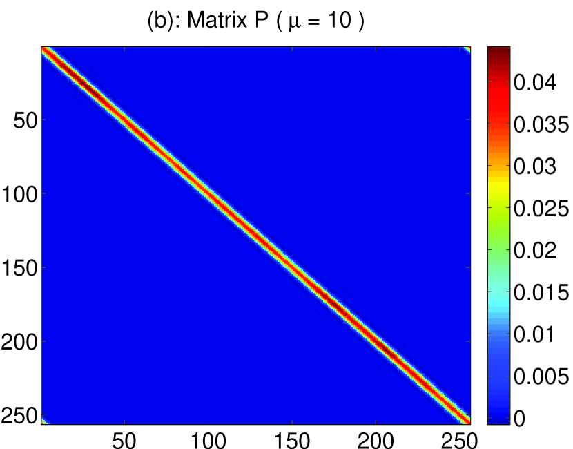
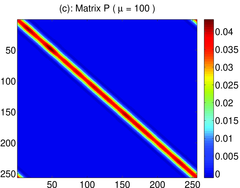
Figure 1. (a): The true density matrix obtained by the first 10 eigenfunctions of $H$. (b), (c): solutions of the density matrices with $\mu=10,100$ respectively.

After we obtain the sparse representation of the density matrix $P$, we can find localized Wannier functions as its action on the delta functions, as plotted in Figure 2 upper and lower pictures for $\mu=10$ and $100$ respectively.

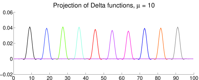
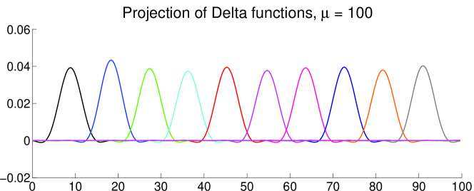
Figure 2. Projection of Delta function $\delta(x-x_{i})$ using density matrices with $\mu=10$ (upper) and $\mu=100$ (lower) respectively.

To indicate the approximation behavior of the proposed model, we consider the energy function approximation of $\frac{1}{\mu}\lVert P\rVert_{1}+\operatorname{tr}(HP)$ to $\sum_{i=1}^{10}\langle\phi_{i}|H|\phi_{i}\rangle$ with different values of $\mu$. In addition, we define $\sum_{i=1}^{10}\|\phi_{i}-P\phi_{i}\|^{2}$ as a measurement for the space approximation of the density matrix $P$ to the lower eigen-space $Span\{\phi_{i}\}_{i=1}^{10}$. Figure 3 reports the energy approximation and the space approximation with different values of $\mu$. Both numerical results suggest that the proposed model will converge to the energy states of the Schrödinger operator. We also remark that even though the exact density matrix is not sparse, a sparse approximation gives fairly good results in terms of energy and space approximations.

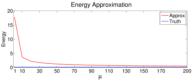
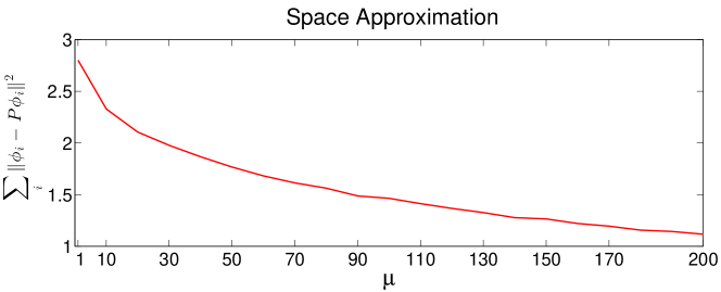
Figure 3. Upper: Energy approximation as a function of $\mu$. Lower: Space approximation as a function of $\mu$.

4.2. 1D Hamiltonian operator with a band gap

We then consider a modified Kronig–Penney (KP) model [Kronig:1931quantum] for a one-dimensional insulator. The original KP model describes the states of independent electrons in a one-dimensional crystal, where the potential function $V(x)$ consists of a periodic array of rectangular potential wells. We replace the rectangular wells with inverted Gaussians so that the potential is given by

$$V(x)=-V_{0}\sum_{j=1}^{N_{\text{at}}}\exp\left[-\frac{(x-x_{j})^{2}}{\delta^{2}}\right],$$

where $N_{\text{at}}$ gives the number of potential wells. In our numerical experiments, we choose $N_{\text{at}}=10$ and $x_{j}=100j/11$ for $j=1,\ldots,N_{\text{at}}$, and the domain is $[0,100]$ with periodic boundary condition. The potential is plotted in Figure 4(a). For this given potential, the Hamiltonian operator $H=-\tfrac{1}{2}\Delta+V(x)$ exhibits two low-energy bands separated by finite gaps from the rest of the eigenvalue spectrum (See Figure 4(b)). Here a centered difference is used to discretize the Hamiltonian operator.

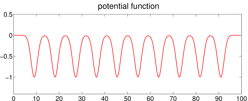
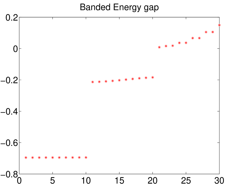
(a)

(b)

Figure 4. (a): The potential function in the modified Kronig-Penney model. (b): The spectrum of the (discretized) Hamiltonian operator.

We consider three choices of $N$ for this model: $N=10$, $N=15$ and $N=20$. They correspond to three interesting physical situations of the model, as explained below.

For $N=10$, the first band of the Hamiltonian is occupied, and hence the system has a spectral gap between the occupied and unoccupied states. As a result, the associated density matrix is exponentially localized, as shown in Figure 5(a). The resulting sparse representation from the convex optimization is shown in Figure 5(b) and (c) for $\mu=10$ and $100$ respectively. We see that the sparse representation agrees well with the exact density matrix, as the latter is very localized. The Wannier functions obtained by projection of delta functions are shown in Figure 6. As the system is an insulator, we see that the localized representation converges quickly to the exact answer when $\mu$ increases. This is further confirmed in Figure 7 where the energy corresponding to the approximated density matrix and space approximation measurement $\sum_{i=1}^{10}\|\phi_{i}-P\phi_{i}\|^{2}$ are plotted as functions of $\mu$.

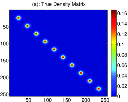
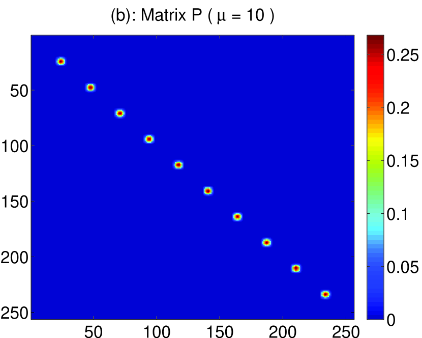
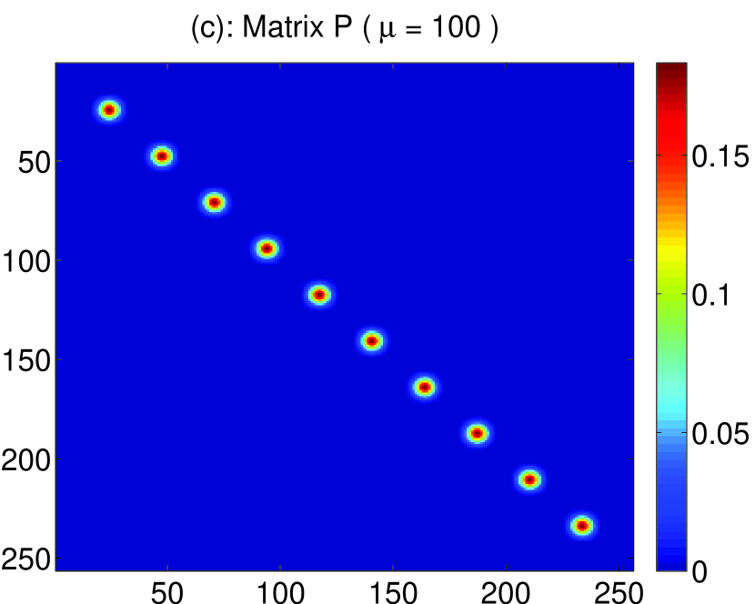
Figure 5. (a): The true density matrix obtained by the first 10 eigenfunctions of $H$. (b), (c): solutions of the density matrices with $\mu=10,100$ respectively.

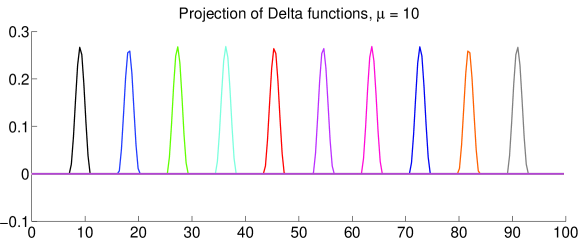
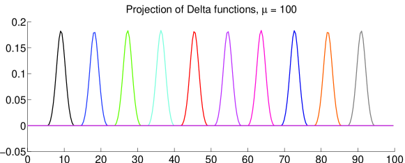
Figure 6. Projection of Delta function $\delta(x-x_{i})$ using density matrices with $\mu=10$ (upper) and $\mu=100$ (lower) respectively.

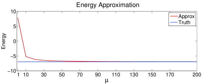
(a)

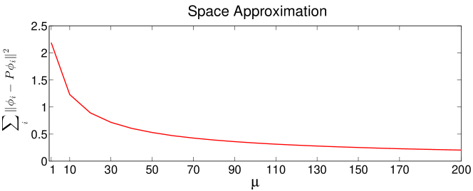
(b)

Figure 7. (a): Energy approximation as a function of $\mu$. (b): Space approximation as a function of $\mu$.

Next we consider the case $N=15$. The first band of $10$ eigenstates of $H$ is occupied and the second band of $H$ is “half-filled”. That is we have only $5$ electrons occupying the $10$ eigenstates of comparable eigenvalue of $H$. Hence, the system does not have a gap, which is indicated by the slow decay of the density matrix shown in Figure 8(a). Nevertheless, the algorithm with $\mu=100$ gives a sparse representation of the density matrix, which captures the feature of the density matrix near the diagonal, as shown in Figure 8(b). To understand better the resulting sparse representation, we diagonal the matrix $P$:

$$P=\sum_{i}f_{i}\varphi_{i}\varphi_{i}^{\mathrm{T}}.$$

The eigenvalues $f_{i}$, known as the occupation number in the physics literature, are sorted in the decreasing order. The first $40$ occupation numbers are shown in Figure 8(c). We have $\sum_{i}f_{i}=\operatorname{tr}P=15$, and we see that $\{f_{i}\}$ exhibits two groups. The first $10$ occupation numbers are equal to $1$, corresponding to the fact that the lowest $10$ eigenstates of the Hamiltonian operator is occupied. Indeed, if we compare the eigenvalues of the operator $PH$ with the eigenvalues of $H$, as in Figure 8(d), we see that the first $10$ low-lying states are well represented in $P$. This is further confirmed by the filtered density matrix $M_{1}$ given by the first $10$ eigenstates of $P$ as

$$M_{1}=\sum_{i=1}^{10}f_{i}\varphi_{i}\varphi_{i}^{\mathrm{T}},$$

plotted in Figure 8(e). It is clear that it is very close to the exact density matrix corresponding to the first $10$ eigenfunctions of $H$, as plotted in Figure 5(a). The next group of occupation numbers in Figure 8(c) gets value close to $0.5$. This indicates that those states are “half-occupied”, matches very well with the physical intuition. This is also confirmed by the state energy shown in Figure 8(d). Note that due to the fact these states are half filled, the perturbation in the eigenvalue by the localization is much stronger. The corresponding filtered density matrix

$$M_{2}=\sum_{i=11}^{20}f_{i}\varphi_{i}\varphi_{i}^{\mathrm{T}},$$

is shown in Figure 8(f).

For this example, we compare with the results obtained using the variational principle (3) as in [OzolinsLaiCaflischOsher:13] shown in Figure 9. As the variational principle (3) is formulated with orbital functions $\Psi$, it does not allow fractional occupations, in contrast with the one in terms of the density matrix. Hence, the occupation number is either $1$ or $0$, which is equivalent to the idempotency condition, as shown in Figure 9(b). As a result, even though the states in the second band have very similar energy, the resulting $\Psi$ are forced to choose five states over the ten, as can be seen from the Ritz value plotted in Figure 9(c). The solution is quite degenerate in this case. Physically, what happens is that the five electrons choose $5$ wells out of the ten to sit in (on top of the state corresponding to the first band already in the well), as shown from the corresponding density matrix in Figure 9(a), or more clearly by the filtered density matrix in Figure 9(d) for the five higher energy states.

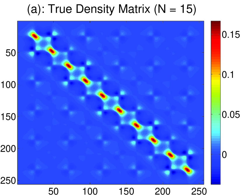
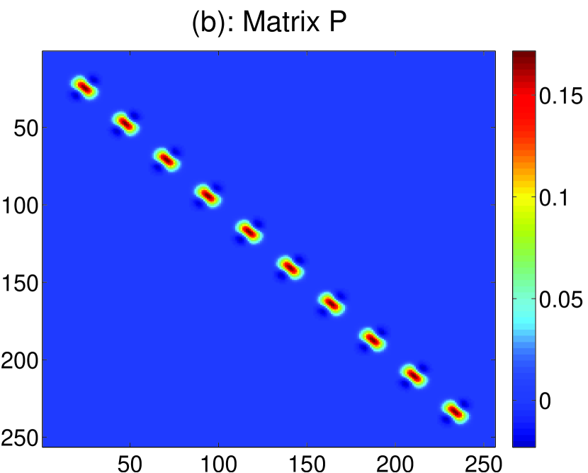
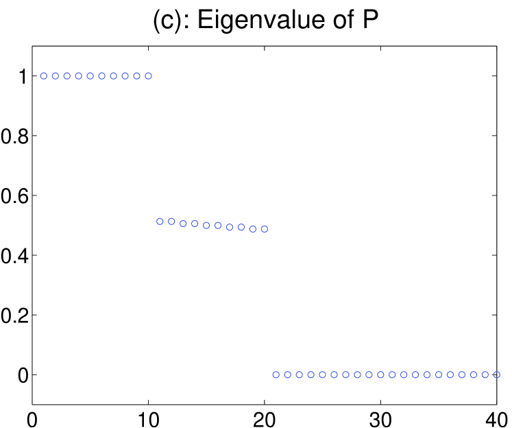
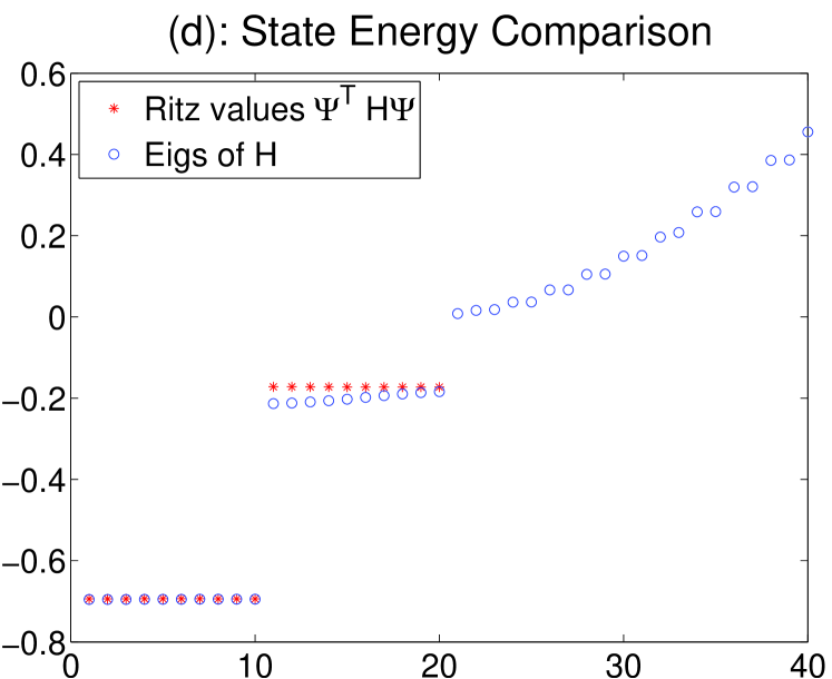
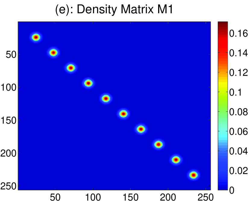
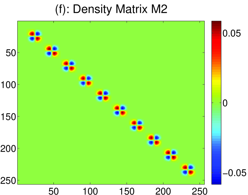
Figure 8. (a): The true density matrix corresponds to the first $15$ eigenfunctions of $H$. (b): The sparse representation $P$ of the density matrix for $\mu=100$. (c): The occupation number (eigenvalues) of $P$. (d) The first $15$ eigenvalues of $PH$ compared with the eigenvalues of $H$. (e): The filtered density matrix $M_{1}$ corresponds to the first $10$ eigenstates of $P$. (f) The filtered density matrix $M_{2}$ corresponds to the next $10$ eigenstates of $P$.

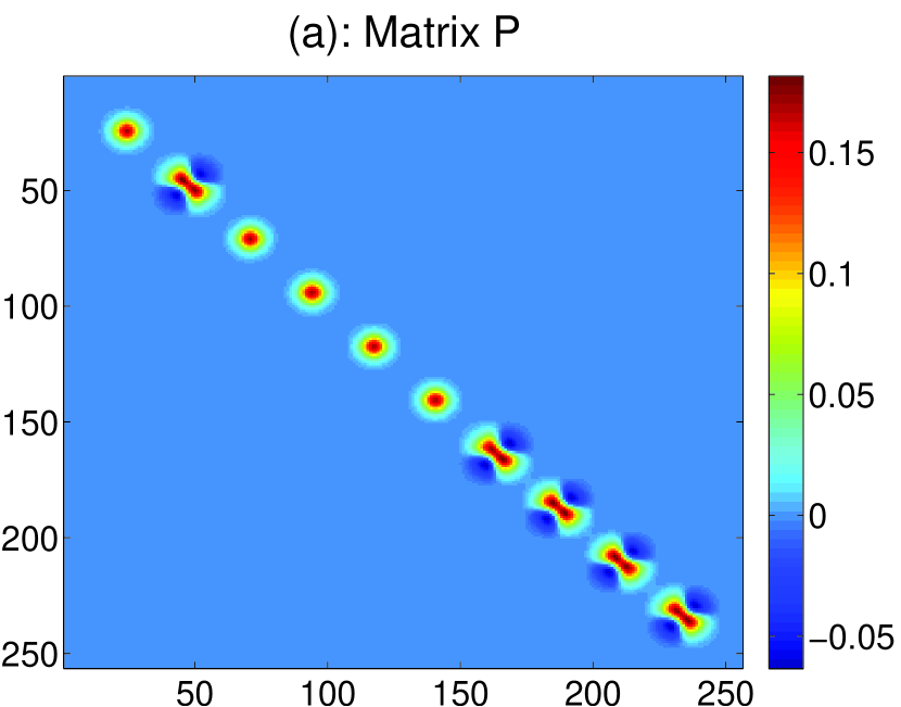
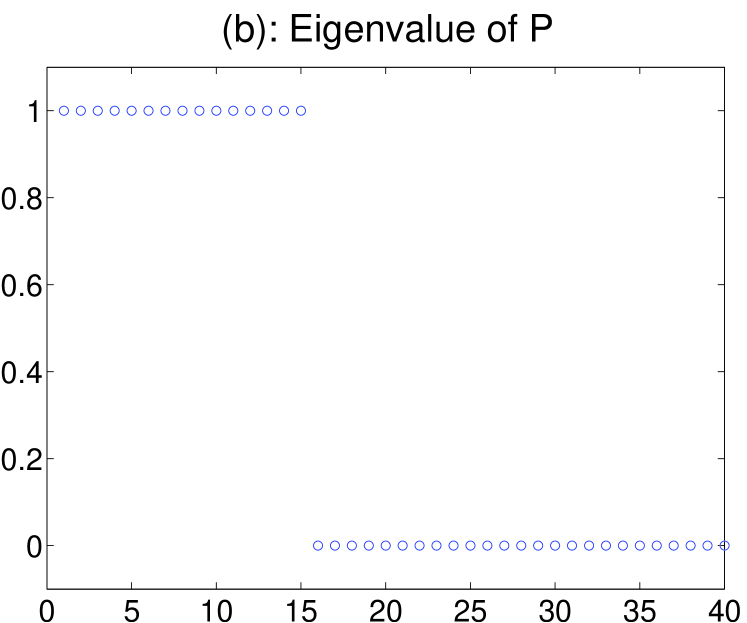
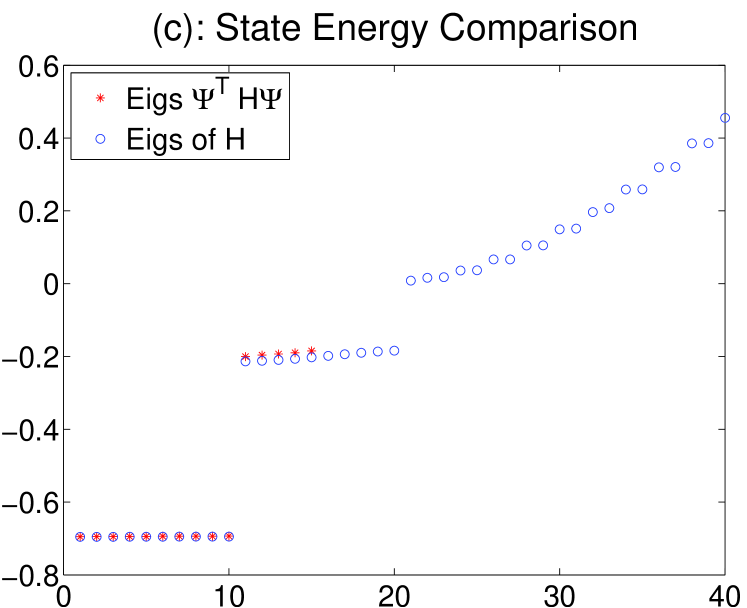
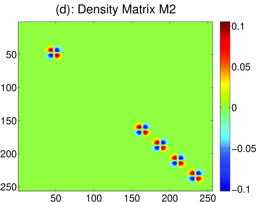
Figure 9. Results obtained by the first 15 Compressed modes $\Psi=\{\psi_{i}\}_{i=1}^{15}$ for $\mu=100$. (a): The density representation $P$ given by $P=\Psi^{T}\Psi$. (b): The occupation number (eigenvalues) of $P$. (d) The first $15$ eigenvalues of $\Psi^{T}H\Psi$ compared with the eigenvalues of $H$. (d) The filtered density matrix $M_{2}$ corresponds to the $5$ states in the second band.

Finally, the $N=20$ case corresponds to the physical situation that the first two bands are all occupied. Note that as the band gap between the second band from the rest of the spectrum is smaller than the gap between the first two bands, the density matrix, while still exponentially localized, has a slower off diagonal decay rate. The exact density matrix corresponds to the first $20$ eigenfunctions of $H$ is shown in Figure 10(a), and the localized representation with $\mu=100$ is given in Figure 10(b). The occupation number is plotted in Figure 10(c), indicates that the first $20$ states are fully occupied, while the rest of the states are empty. This is further confirmed by comparison of the eigenvalues given by $HP$ and $H$, shown in Figure 10(d). In this case, we see that physically, each well contains two states. Hence, if we look at the electron density, which is diagonal of the density matrix, we see a double peak in each well. Using the projection of delta functions, we see that the sparse representation of the density matrix $P$ automatically locate the two localized orbitals centered at the two peaks, as shown in Figure 10(e).

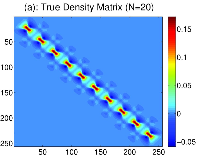
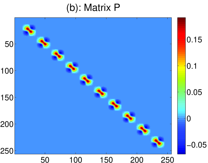
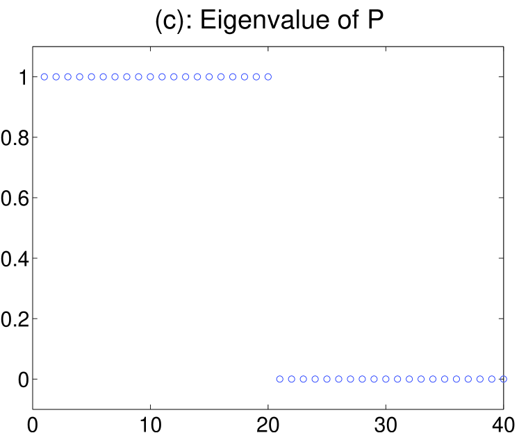
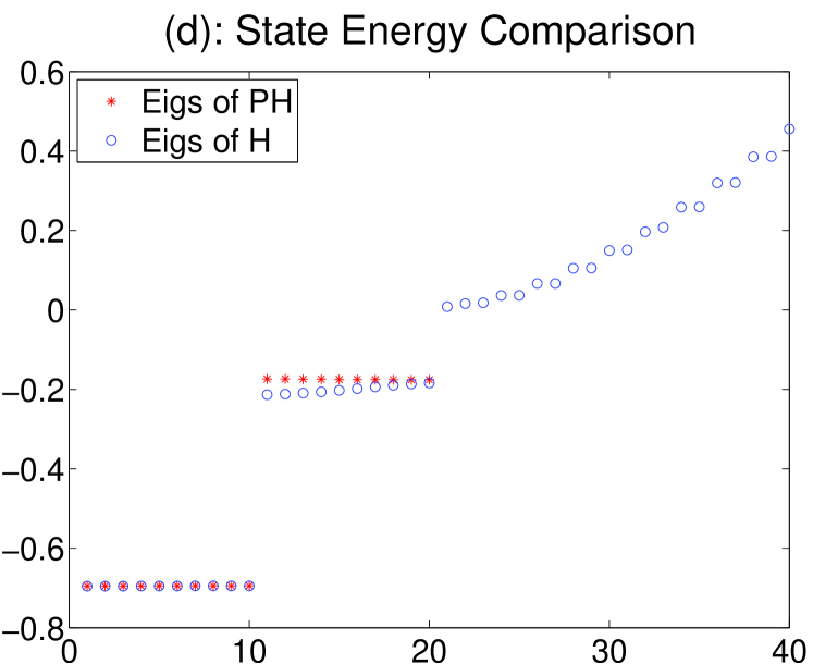
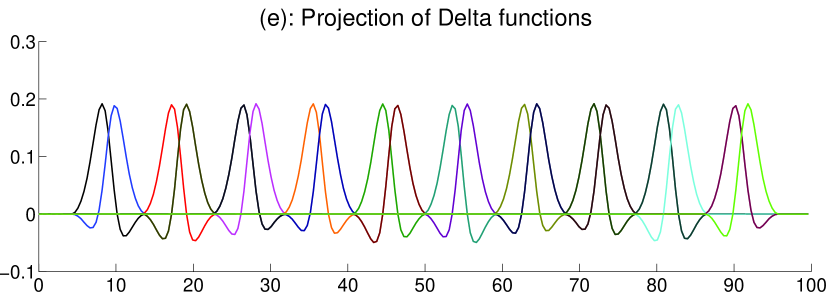
Figure 10. (a): The true density matrix corresponds to the first $20$ eigenfunctions of $H$. (b): The sparse representation $P$ of the density matrix for $\mu=100$. (c): The occupation number (eigenvalues) of $P$. (d) The first $20$ eigenvalues of $PH$ compared with the eigenvalues of $H$. (e) Projection of Delta function $\delta(x-x_{i})$.

4.3. An example of non-unique minimizers

Let us revisit the Example $2$ in Section 2 for which the minimizers to the variational problem is non-unique. Theorem 3 guarantees that the algorithm will converge to some minimizer starting from any initial condition.

It is easy to check that in this case

(22) $$P^{\ast}=Q^{\ast}=R^{\ast}=\begin{pmatrix}1&0&0\\ 0&0&0\\ 0&0&0\end{pmatrix},\quad b^{\ast}=\begin{pmatrix}1&0&0\\ 0&1&-1\\ 0&-1&1\end{pmatrix},\quad d^{\ast}=\begin{pmatrix}0&0&0\\ 0&-1&-1\\ 0&-1&-1\end{pmatrix}$$

is a fixed point of the algorithm. In Figure 11, we plot the sequence $\Big{\{}\lambda\|b^{k}-b^{\ast}\|^{2}+r\|d^{k}-d^{\ast}\|^{2}+\lambda\|Q^{k}-Q^{\ast}\|^{2}+r\|R^{k}-R^{\ast}\|^{2}\Big{\}}_{k}$ for a randomly chosen initial data. We see that the distance does not converge to $0$ as the algorithm converges to another minimizer of the variational problem. Nonetheless, as will be shown in the proof of Theorem 3 in Section 5, the sequence is monotonically non-increasing.

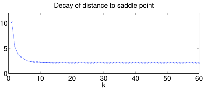
Figure 11. $\lambda\|b^{k}-b^{\ast}\|^{2}+r\|d^{k}-d^{\ast}\|^{2}+\lambda\|Q^{k}-Q^{\ast}\|^{2}+r\|R^{k}-R^{\ast}\|^{2}$ as a function of $k$ for Algorithm 2.

5. Convergence of Algorithm 2

For ease of notation, we will prove the convergence of the algorithm for the following slightly generalized variational problem.

(23) $$\min_{P,Q,R}f(P)+g(Q)+h(R)$$

$$\text{s.t.}\;P=Q,P=R$$

where $f$, $g$, and $h$ are proper convex functionals, but not necessarily strictly convex. In particular, we will get (15) if we set

$$f(P)=\begin{cases}\operatorname{tr}(HP),&\text{if }\operatorname{tr}P=N;\\ +\infty,&\text{otherwise},\end{cases}$$

$$g(Q)=\lVert Q\rVert_{1}/\mu$$

$$h(R)=\begin{cases}0,&\text{if }R=R^{\mathrm{T}},\text{and }0\preceq R\preceq I;\\ +\infty,&\text{otherwise}.\end{cases}$$

The corresponding algorithm for (23) is given by

Algorithm 4.

Initialize $P^{0}=Q^{0}=R^{0},b^{0}=d^{0}=0$

while “not converge” do

      

1. $\displaystyle P^{k}=\arg\min_{P}f(P)+\frac{\lambda}{2}\lVert P-Q^{k-1}+b^{k-1}\rVert^{2}+\frac{r}{2}\lVert P-R^{k-1}+d^{k-1}\rVert^{2}$,

2. $\displaystyle Q^{k}=\arg\min_{Q}g(Q)+\frac{\lambda}{2}\lVert P^{k}-Q+b^{k-1}\rVert^{2}$.

3. $R^{k}=\displaystyle\arg\min_{R}h(R)+\frac{r}{2}\lVert P^{k}-R+d^{k-1}\rVert^{2}$.

4. $b^{k}=b^{k-1}+P^{k}-Q^{k}$.

5. $d^{k}=d^{k-1}+P^{k}-R^{k}$.

We define an augmented Lagrangian

(24) $$\mathcal{L}(P,Q,R;b,d)=f(P)+g(Q)+h(R)+\frac{\lambda}{2}\|P-Q\|^{2}+\lambda\langle P-Q,b\rangle\\ +\frac{r}{2}\|P-R\|^{2}+r\langle P-R,d\rangle$$

Definition 5.

We call $(P^{\ast},Q^{\ast},R^{\ast};b^{\ast},d^{\ast})$ a saddle point of the Lagrangian (24), if

(25) $$\mathcal{L}(P^{\ast},Q^{\ast},R^{\ast};b,d)\leq\mathcal{L}(P^{\ast},Q^{\ast},R^{\ast};b^{\ast},d^{\ast})\leq\mathcal{L}(P,Q,R;b^{\ast},d^{\ast})$$

for any $(P,Q,R;b,d)\in\mathbb{R}^{n\times n}\times\mathbb{R}^{n\times n}\times\mathbb{R}^{n\times n}\times\mathbb{R}^{n\times n}\times\mathbb{R}^{n\times n}$.

Lemma 1.

$(P^{*},Q^{*},R^{*})$ is a solution of the optimization problem (23) if any only if there exist $b^{*},d^{*}\in\mathbb{R}^{n\times n}$ such that $(P^{*},Q^{*},R^{*};b^{*},d^{*})$ is a saddle point satisfying (25)

Proof.

Given a saddle point $(P^{*},Q^{*},R^{*};b^{*},d^{*})$ satisfying (25), it is clear that the first inequality in (25) implies $P^{*}=Q^{*}=R^{*}$. Substitute $P=Q=R$ in the second inequality of (25), we can immediately have $(P^{*},Q^{*},R^{*})$ is a minimizer (23).

On the other hand, suppose $(P^{*},Q^{*},R^{*})$ is a solution of (23). The first inequality in (25) holds since $P^{*}=Q^{*}=R^{*}$. Moreover, there exist $b^{*},d^{*}$ such that

$$-\lambda b^{*}-rd^{*}\in\partial f(P^{*}),\qquad\lambda b^{*}\in\partial g(Q^{*}),\qquad rd^{*}\in\partial h(R^{*})$$

which suggests, for any $P,Q,R\in\mathbb{R}^{n\times n}$

$$f(P^{*}) \leq f(P)+\lambda\langle b^{*},P-P^{*}\rangle+r\langle d^{*},P-P^{*}\rangle$$

$$g(Q^{*}) \leq g(Q)-\lambda\langle b^{*},Q-Q^{*}\rangle$$

$$h(R^{*}) \leq h(R)-r\langle d^{*},R-R^{*}\rangle$$

The summation of the above three inequalities yield the second inequality in (25). ∎

Theorem 6.

The sequence $\Big{\{}(P^{k},Q^{k},R^{k})\Big{\}}_{k}$ generated by Algorithm 4 from any starting point converges to a minimum of the variational problem (23).

Remark.

We remind the readers that the minimizers of the variational principle (23) might not be unique. In the non-unique case, the above theorem states that any initial condition will converge to some minimizer, while different initial condition might give different minimizers.

Proof.

Let $(P^{\ast},Q^{\ast},R^{\ast})$ be an optimal solution of (23). We introduce the short hand notations

(26) $$\begin{split}&\widebar{P}^{k}=P^{k}-P^{*},\quad\widebar{Q}^{k}=Q^{k}-Q^{*},\quad\text{and}\quad\widebar{R}^{k}=R^{k}-R^{*}.\\ &\widebar{b}^{k}=b^{k}-b^{*},\quad\widebar{d}^{k}=d^{k}-d^{*}.\end{split}$$

From Step $4$ and $5$ in the algorithm, we get

(27) $$\widebar{b}^{k}=\widebar{b}^{k-1}+\widebar{P}^{k}-\widebar{Q}^{k},\quad\text{and}\quad\widebar{d}^{k}=\widebar{d}^{k-1}+\widebar{P}^{k}-\widebar{R}^{k},$$

and hence

(28) $$\begin{split}&\|\widebar{b}^{k-1}\|^{2}-\|\widebar{b}^{k}\|^{2}=-2\langle\widebar{b}^{k-1},\widebar{P}^{k}-\widebar{Q}^{k}\rangle-\|\widebar{P}^{k}-\widebar{Q}^{k}\|^{2}\\ &\lVert\widebar{d}^{k-1}\rVert^{2}-\|\widebar{d}^{k}\|^{2}=-2\langle\widebar{d}^{k-1},\widebar{P}^{k}-\widebar{R}^{k}\rangle-\|\widebar{P}^{k}-\widebar{R}^{k}\|^{2}\end{split}$$

Note that by optimality

(29) $$P^{*}=\arg\min_{P\in\mathcal{C}_{P}}\mathcal{L}(P,Q^{*},R^{*};b^{*},d^{*})$$

(30) $$Q^{*}=\arg\min_{Q\in\mathcal{C}_{Q}}\mathcal{L}(P^{*},Q,R^{*};b^{*},d^{*})$$

(31) $$R^{*}=\arg\min_{R\in\mathcal{C}_{R}}\mathcal{L}(P^{*},Q^{*},R;b^{*},d^{*})$$

Hence, for any $P,Q,R\in\mathbb{R}^{n\times n}$, we have

(32) $$f(P)-f(P^{*})+\lambda\langle P^{*}-Q^{*}+b^{*},P-P^{*}\rangle+r\langle P^{*}-R^{*}+d^{*},P-P^{*}\rangle\geq 0$$

(33) $$g(Q)-g(Q^{*})+\lambda\langle Q^{*}-P^{*}-b^{*},Q-Q^{*}\rangle\geq 0$$

(34) $$h(R)-h(R^{*})+r\langle R^{*}-P^{*}-d^{*},R-R^{*}\rangle\geq 0$$

According to the construction of $\{P^{k},Q^{k},R^{k}\}$, for any $P,Q,R\in\mathbb{R}^{n\times n}$, we have

(35) $$\begin{aligned} f(P)-f(P^{k})&+\lambda\langle P^{k}-Q^{k-1}+b^{k-1},P-P^{k}\rangle\\ &+r\langle P^{k}-R^{k}+d^{k-1},P-P^{k}\rangle\geq 0\end{aligned}$$

(36) $$g(Q)-g(Q^{k})+\lambda\langle Q^{k}-P^{k}-b^{k-1},Q-Q^{k}\rangle\geq 0$$

(37) $$h(R)-h(R^{k})+r\langle R^{k}-P^{k}-d^{k-1},R-R^{k}\rangle\geq 0$$

Let $P=P^{k}$ in (32) and $P=P^{*}$ in (35), their summation yields

(38) $$\lambda\langle-\widebar{P}^{k}+\widebar{Q}^{k-1}-\widebar{b}^{k-1},\widebar{P}^{k}\rangle+r\langle-\widebar{P}^{k}+\widebar{R}^{k-1}-\widebar{d}^{k-1},\widebar{P}^{k}\rangle\geq 0$$

Similarly, let $Q=Q^{k}$ in (33) and $Q=Q^{*}$ in (36), and let $R=R^{k}$ in (34) and $R=R^{*}$ in (37), we obtain

(39) $$\lambda\langle-\widebar{Q}^{k}+\widebar{P}^{k}+\widebar{b}^{k-1},\widebar{Q}^{k}\rangle\geq 0$$

(40) $$r\langle-\widebar{R}^{k}+\widebar{P}^{k}+\widebar{d}^{k-1},\widebar{R}^{k}\rangle\geq 0$$

The summation of (38), (39), and (40) yields

(41) $$\lambda\langle-\widebar{b}^{k-1},\widebar{P}^{k}\rangle+\lambda\langle\widebar{Q}^{k-1}-\widebar{P}^{k},\widebar{P}^{k}\rangle+r\langle-\widebar{d}^{k-1},\widebar{P}^{k}\rangle+r\langle\widebar{R}^{k-1}-\widebar{P}^{k},\widebar{P}^{k}\rangle\\ +\lambda\langle\widebar{b}^{k-1},\widebar{Q}^{k}\rangle+\lambda\langle\widebar{P}^{k}-\widebar{Q}^{k},\widebar{Q}^{k}\rangle+r\langle\widebar{d}^{k-1},\widebar{R}^{k}\rangle+r\langle\widebar{P}^{k}-\widebar{R}^{k},\widebar{R}^{k}\rangle\geq 0.$$

This gives us, after organizing terms

(42) $$-\lambda\langle\widebar{b}^{k-1},\widebar{P}^{k}-\widebar{Q}^{k}\rangle-\lambda\|\widebar{Q}^{k}-\widebar{P}^{k}\|^{2}-\lambda\langle\widebar{P}^{k},\widebar{Q}^{k}-\widebar{Q}^{k-1}\rangle\\ -r\langle\widebar{d}^{k-1},\widebar{P}^{k}-\widebar{R}^{k}\rangle-r\|\widebar{R}^{k}-\widebar{P}^{k}\|^{2}-r\langle\widebar{P}^{k},\widebar{R}^{k}-\widebar{R}^{k-1}\rangle\geq 0$$

Combining the above inequality with (28), we have

(43) $$\bigl{(}\lambda\|\widebar{b}^{k-1}\|^{2}+r\|\widebar{d}^{k-1}\|^{2}\bigr{)} -\bigl{(}\lambda\|\widebar{b}^{k}\|^{2}+r\|\widebar{d}^{k}\|^{2}\bigr{)}$$

$$=\lambda\bigl{(}-2\langle\widebar{b}^{k-1},\widebar{P}^{k}-\widebar{Q}^{k}\rangle-\|\widebar{P}^{k}-\widebar{Q}^{k}\|^{2}\bigr{)}$$

$$\qquad+r\bigl{(}-2\langle\widebar{d}^{k-1},\widebar{P}^{k}-\widebar{R}^{k}\rangle-\|\widebar{P}^{k}-\widebar{R}^{k}\|^{2}\bigr{)}$$

$$\geq\lambda\|\widebar{Q}^{k}-\widebar{P}^{k}\|^{2}+2\lambda\langle\widebar{P}^{k},\widebar{Q}^{k}-\widebar{Q}^{k-1}\rangle$$

$$\qquad+r\|\widebar{R}^{k}-\widebar{P}^{k}\|^{2}+2r\langle\widebar{P}^{k},\widebar{R}^{k}-\widebar{R}^{k-1}\rangle$$

Now, we calculate $\langle\widebar{P}^{k},\widebar{Q}^{k}-\widebar{Q}^{k-1}\rangle$. It is clear that

(44) $$\langle\widebar{P}^{k},\widebar{Q}^{k}-\widebar{Q}^{k-1}\rangle=\langle\widebar{P}^{k}-\widebar{P}^{k-1},\widebar{Q}^{k}-\widebar{Q}^{k-1}\rangle+\langle\widebar{P}^{k-1}-\widebar{Q}^{k-1},\widebar{Q}^{k}-\widebar{Q}^{k-1}\rangle\\ +\langle\widebar{Q}^{k-1},\widebar{Q}^{k}-\widebar{Q}^{k-1}\rangle$$

Note that $\displaystyle Q^{k-1}=\arg\min_{Q}g(Q)+\frac{\lambda}{2}\|Q-P^{k-1}-b^{k-2}\|^{2}$. Thus, for any $Q\in\mathbb{R}^{n\times n}$, we have

(45) $$g(Q)-g(Q^{k-1})+\lambda\langle Q^{k-1}-P^{k-1}-b^{k-2},Q-Q^{k-1}\rangle\geq 0$$

In particular, let $Q=Q^{k}$, we have

(46) $$g(Q^{k})-g(Q^{k-1})+\lambda\langle Q^{k-1}-P^{k-1}-b^{k-2},Q^{k}-Q^{k-1}\rangle\geq 0$$

On the other hand, set $Q=Q^{k-1}$ in (36), we get

(47) $$g(Q^{k-1})-g(Q^{k})+\lambda\langle Q^{k}-P^{k}-b^{k-1},Q^{k-1}-Q^{k}\rangle\geq 0$$

The summation of (46) and (47) yields

(48) $$\langle b^{k-1}-b^{k-2},Q^{k}-Q^{k-1}\rangle+\langle Q^{k-1}-Q^{k}+P^{k}-P^{k-1},Q^{k}-Q^{k-1}\rangle\geq 0$$

Note that $P^{k}-P^{k-1}=\widebar{P}^{k}-\widebar{P}^{k-1},Q^{k}-Q^{k-1}=\widebar{Q}^{k}-\widebar{Q}^{k-1},b^{k-1}-b^{k-2}=\widebar{P}^{k-1}-\widebar{Q}^{k-1}$, thus we have

(49) $$\langle\widebar{P}^{k-1}-\widebar{Q}^{k-1},\widebar{Q}^{k}-\widebar{Q}^{k-1}\rangle+\langle\widebar{P}^{k}-\widebar{P}^{k-1},\widebar{Q}^{k}-\widebar{Q}^{k-1}\rangle\geq\|\widebar{Q}^{k}-\widebar{Q}^{k-1}\|^{2}$$

Combine (49) with (44), we have

(50) $$\langle\widebar{P}^{k},\widebar{Q}^{k}-\widebar{Q}^{k-1}\rangle\geq\|\widebar{Q}^{k}-\widebar{Q}^{k-1}\|^{2}+\langle\widebar{Q}^{k-1},\widebar{Q}^{k}-\widebar{Q}^{k-1}\rangle$$

Similarly, we have

(51) $$\langle\widebar{P}^{k},\widebar{R}^{k}-\widebar{R}^{k-1}\rangle\geq\|\widebar{R}^{k}-\widebar{R}^{k-1}\|^{2}+\langle\widebar{R}^{k-1},\widebar{R}^{k}-\widebar{R}^{k-1}\rangle$$

Substitute (50) and (51) into (43), we have

(52) $$\bigl{(}\lambda\|\widebar{b}^{k-1}\|^{2}+r\|\widebar{d}^{k-1}\|^{2}) -(\lambda\|\widebar{b}^{k}\|^{2}+r\|\widebar{d}^{k}\|^{2})$$

$$\geq\lambda\|\widebar{Q}^{k}-\widebar{P}^{k}\|^{2}+2\lambda\langle\widebar{P}^{k},\widebar{Q}^{k}-\widebar{Q}^{k-1}\rangle$$

$$\qquad+r\|\widebar{R}^{k}-\widebar{P}^{k}\|^{2}+2r\langle\widebar{P}^{k},\widebar{R}^{k}-\widebar{R}^{k-1}\rangle$$

$$\geq\lambda\|\widebar{Q}^{k}-\widebar{P}^{k}\|^{2}+2\lambda\bigl{(}\|\widebar{Q}^{k}-\widebar{Q}^{k-1}\|^{2}+\langle\widebar{Q}^{k-1},\widebar{Q}^{k}-\widebar{Q}^{k-1}\rangle\bigr{)}$$

$$\qquad+r\|\widebar{R}^{k}-\widebar{P}^{k}\|^{2}+2r\bigl{(}\|\widebar{R}^{k}-\widebar{R}^{k-1}\|^{2}+\langle\widebar{R}^{k-1},\widebar{R}^{k}-\widebar{R}^{k-1}\rangle\bigr{)}$$

$$=\lambda\|\widebar{Q}^{k}-\widebar{P}^{k}\|^{2}+\lambda\bigl{(}\|\widebar{Q}^{k}\|^{2}-\|\widebar{Q}^{k-1}\|^{2}+\|\widebar{Q}^{k}-\widebar{Q}^{k-1}\|^{2}\bigr{)}$$

$$\qquad+r\|\widebar{R}^{k}-\widebar{P}^{k}\|^{2}+r\bigl{(}\|\widebar{R}^{k}\|^{2}-\|\widebar{R}^{k-1}\|^{2}+\|\widebar{R}^{k}-\widebar{R}^{k-1}\|^{2}\bigr{)}$$

which yields

(53) $$\bigl{(}\lambda\|\widebar{b}^{k-1}\|^{2}+r\|\widebar{d}^{k-1}\|^{2}+\lambda\|\widebar{Q}^{k-1}\|^{2}+r\|\widebar{R}^{k-1}\|^{2}\bigr{)}\\ -\bigl{(}\lambda\|\widebar{b}^{k}\|^{2}+r\|\widebar{d}^{k}\|^{2}+\lambda\|\widebar{Q}^{k}\|^{2}+r\|\widebar{R}^{k}\|^{2}\bigr{)}\\ \geq\lambda\|\widebar{Q}^{k}-\widebar{P}^{k}\|^{2}+\lambda\|\widebar{Q}^{k}-\widebar{Q}^{k-1}\|^{2}+r\|\widebar{R}^{k}-\widebar{P}^{k}\|^{2}+r\|\widebar{R}^{k}-\widebar{R}^{k-1}\|^{2}$$

This concludes that the sequence $\Big{\{}\lambda\|\widebar{b}^{k}\|^{2}+r\|\widebar{d}^{k}\|^{2}+\lambda\|\widebar{Q}^{k}\|^{2}+r\|\widebar{R}^{k}\|^{2}\Big{\}}_{k}$ is non-increasing and hence convergent. This further implies,

1. $\{P^{k}\}_{k},\{Q^{k}\}_{k},\{R^{k}\}_{k},\{b^{k}\}_{k},\{d^{k}\}_{k}$ are all bounded sequences, and hence the sequences has limit points.

2. $\lim_{k\rightarrow\infty}\|Q^{k}-P^{k}\|=0$ and $\lim_{k\rightarrow\infty}\|R^{k}-P^{k}\|=0$.

Therefore, the sequences have limit points. Let us denote $(\widetilde{P},\widetilde{Q},\widetilde{R};\widetilde{b},\widetilde{d})$ as a limit point, that is, a subsequence converges

(54) $$\lim_{j\to\infty}(P^{k_{j}},Q^{k_{j}},R^{k_{j}};b^{k_{j}},d^{k_{j}})=(\widetilde{P},\widetilde{Q},\widetilde{R};\widetilde{b},\widetilde{d}).$$

We now prove that $(\widetilde{P},\widetilde{Q},\widetilde{R})$ is a minimum of the variational problem (23), i.e.

(55) $$f(\widetilde{P})+g(\widetilde{Q})+h(\widetilde{R})=\lim_{j\rightarrow\infty}f(P^{k_{j}})+g(Q^{k_{j}})+h(R^{k_{j}})=f(P^{*})+g(Q^{*})+h(R^{*})$$

First note that since $(P^{*},Q^{*},R^{*};b^{*},d^{*})$ is a saddle point, we have

(56) $$f(P^{*})+g(Q^{*})+h(R^{*})\leq f(P^{k_{j}})+g(Q^{k_{j}})+h(R^{k_{j}})+\frac{\lambda}{2}\|P^{k_{j}}-Q^{k_{j}}\|^{2}\\ +\lambda\langle P^{k_{j}}-Q^{k_{j}},b^{*}\rangle+\frac{r}{2}\|P^{k_{j}}-R^{k_{j}}\|^{2}+r\langle P^{k_{j}}-R^{k_{j}},d^{*}\rangle$$

Taking the limit $j\to\infty$, we get

(57) $$f(P^{*})+g(Q^{*})+h(R^{*})\leq f(\widetilde{P})+g(\widetilde{Q})+h(\widetilde{R}).$$

On the other hand, taking $P=P^{*}$, $Q=Q^{*}$, and $R=R^{*}$ in (35)–(37), we get

$$f(P^{*}) +g(Q^{*})+h(R^{*})$$

$$\geq f(P^{k_{j}})+g(Q^{k_{j}})+h(R^{k_{j}})-\lambda\langle P^{k_{j}}-Q^{k_{j}-1}+b^{k_{j}-1},P^{*}-P^{k_{j}}\rangle$$

$$\qquad-r\langle P^{k_{j}}-R^{k_{j}}+d^{k_{j}-1},P^{*}-P^{k_{j}}\rangle-\lambda\langle Q^{k_{j}}-P^{k_{j}}-b^{k_{j}-1},Q^{*}-Q^{k_{j}}\rangle$$

$$\qquad-r\langle R^{k_{j}}-P^{k_{j}}-d^{k_{j}-1},R^{*}-R^{k_{j}}\rangle$$

$$=f(P^{k_{j}})+g(Q^{k_{j}})+h(R^{k_{j}})$$

$$\qquad-\lambda\langle b^{k_{j}-1},Q^{k_{j}}-P^{k_{j}}\rangle-\lambda\langle P^{k_{j}}-Q^{k_{j}-1},P^{*}-P^{k_{j}}\rangle-\lambda\langle Q^{k_{j}}-P^{k_{j}},Q^{*}-Q^{k_{j}}\rangle$$

$$\qquad-r\langle d^{k_{j}-1},R^{k_{j}}-P^{k_{j}}\rangle-r\langle P^{k_{j}}-R^{k_{j}},P^{*}-P^{k_{j}}\rangle-r\langle R^{k_{j}}-P^{k_{j}},R^{*}-R^{k_{j}}\rangle$$

From (53), we have $\{P^{k_{j}}\},\{Q^{k_{j}}\},\{R^{k_{j}}\},\{b^{k_{j}}\},\{d^{k_{j}}\}$ are all bounded sequences, and furthermore,

$$\lim_{j\rightarrow\infty}\|Q^{k_{j}}-P^{k_{j}}\|=0,\qquad\lim_{j\rightarrow\infty}\|Q^{k_{j}}-Q^{k_{j}-1}\|=0.$$

$$\lim_{j\rightarrow\infty}\|R^{k_{j}}-P^{k_{j}}\|=0,\qquad\lim_{j\rightarrow\infty}\|R^{k_{j}}-R^{k_{j}-1}\|=0.$$

Taking the limit $j\to\infty$, we then get

(58) $$f(P^{*})+g(Q^{*})+h(R^{*})\geq f(\widetilde{P})+g(\widetilde{Q})+h(\widetilde{R}).$$

Hence, the limit point is a minimizer of the variational principle.

Finally, repeating the derivation of (53) by replacing $(P^{*},Q^{*},R^{*})$ by $(\widetilde{P},\widetilde{Q},\widetilde{R})$, we get convergence of the whole sequence due to the monotonicity. ∎