An impact model of the electrostatic force:
Coulomb’s law re-visited

Abstract

The electrostatic force is described in this model by the action of electric dipole distributions on charged particles. The individual hypothetical dipoles are propagating at the speed of light in vacuum transferring momentum and energy between charges through interactions on a local basis. The model is constructed in analogy to an impact model describing the gravitational forces.

1 Introduction

Electrostatic fields can be described by a subset of Maxwell’s equations:

$$\oint\mbox{\boldmath$E$}\,{\ \mathrm{d}}\mbox{\boldmath$s$}=0\quad{\rm and}\quad\varepsilon_{0}\int\!\!\!\int_{F}\mbox{\boldmath$E$}\,{\ \mathrm{d}}\mbox{\boldmath$f$}=Q_{F}~{}.$$ (1)

$E$ is the electric field strength, d$s$ an element along a closed integration path, d$f$ an element of the closed surface $F$ of a macroscopic volume with its normal directed outwards, $Q_{F}$ the total electric charge enclosed by $F$, and $\varepsilon_{0}=8.854...~{}\times~{}10^{-12}~{}{\rm F}\,{\ \mathrm{m}}^{-1}$ the electric constant in vacuum. Experience has shown that electric monopoles – either as positive or negative charges –  are attached to matter, and that $Q_{F}$ is zero in vacuum.

For two particles A and B charged with $Q$ and $q$, respectively, at a separation distance, $r$, (large compared to the sizes of the particles) and at rest in an inertial system, Coulomb’s law yields an electrostatic force, $\mbox{\boldmath$K$}_{\rm E}$, acting on $q$ of

$$\mbox{\boldmath$K$}_{\rm E}(\mbox{\boldmath$r$})=\frac{Q\,\hat{\mbox{\boldmath$r$}}}{4\,\pi\,r^{2}\,\varepsilon_{0}}~{}q~{},$$ (2)

where $\hat{\mbox{\boldmath$r$}}$ is the unit vector of the radius vector $r$ from A to B, and $r=|\mbox{\boldmath$r$}|$. If $Q$ and $q$ have opposite signs, the force is an attraction, otherwise a repulsion. The first term on the right-hand side

$$\frac{Q\,\hat{\mbox{\boldmath$r$}}}{4\,\pi\,r^{2}\,\varepsilon_{0}}=\mbox{\boldmath$E$}_{Q}(\mbox{\boldmath$r$})$$ (3)

represents the classical electric field of a charge $Q$. Provided $|q|\ll|Q|$, the total field will not be influenced by $q$ very much. The electric potential, $U(r)$, of a charge, $Q$, located at $r=0$ is

$$U_{Q}(r)=\frac{Q}{4\,\pi\,\varepsilon_{0}~{}r}$$ (4)

for $r>0$. The corresponding electric field can be written as $\mbox{\boldmath$E$}_{Q}(\mbox{\boldmath$r$})=-\nabla U_{Q}(r)$. Eq. (4) indicates that an electric point source cannot be real in a classical theory, and a distribution of the charge within a certain volume must be assumed (cf. e. g. Levine et al., 1977; Rohrlich, 1997, and references cited therein). The energy density of an electric field outside of charges is given by

$$w=\frac{\varepsilon_{0}}{2}\,\mbox{\boldmath$E$}^{2}~{}.$$ (5)

Eqs. (1) to (5) are treated in most physics textbooks (cf. e. g. Hund, 1957; Jackson, 2006). For a single charge, $Q$, the integration of the energy contributions ${\ \mathrm{d}}W_{Q}=w\,{\ \mathrm{d}}V=4\,\pi\,r^{2}\,w\,{\ \mathrm{d}}r$ from $r=\mathrm{\Delta}r$ to $r\to\infty$ yields the total field energy outside the sphere with radius $\mathrm{\Delta}r$

$$W_{Q}(\mathrm{\Delta}r)=\frac{Q^{2}}{8\,\pi\,\varepsilon_{0}}\,\int^{\infty}_{\mathrm{\Delta}r}\frac{{\ \mathrm{d}}r}{r^{2}}=\frac{Q^{2}}{8\,\pi\,\varepsilon_{0}}\,\frac{1}{\mathrm{\Delta}r}~{}.$$ (6)

With $Q=\pm\,|e|=\pm\,1.602\ldots\times 10^{-19}$ C, the elementary charge, and $\mathrm{\Delta}r$ the Bohr radius

$$a_{0}=\frac{\varepsilon_{0}\,h^{2}}{\pi\,m_{\rm e}\,e^{2}}=52.9~{}{\rm pm}~{},$$ (7)

where $m_{\rm e}=9.109\ldots\times 10^{-31}$ kg is the electron mass and $h=6.626\ldots\times 10^{-34}$ J s the Planck constant, Eq. (6) yields

$$W_{\rm e}(a_{0})=\frac{1}{2}\,\alpha^{2}\,m_{\rm e}\,c^{2}_{0}~{},$$ (8)

with $c_{0}=299\,792\,458~{}{\ \mathrm{m}}\,{\ \mathrm{s}}^{-1}$, the speed of light in vacuum, and Sommerfeld’s fine-structure constant

$$\alpha=\frac{e^{2}}{2\,\varepsilon_{0}\,h\,c_{0}}=7.297\ldots\times 10^{-3}~{}.$$ (9)

Laboratory limits for potential temporal drifts of the fine-structure constant $\alpha$ are given by Hänsch et al. (2005); Levshakov (2004). They are consistent with a null result.

Choosing $\mathrm{\Delta}r=\hbar/(m_{\rm e}\,c_{0})=0.386$ pm, the reduced Compton wavelength of an electron, where $\hbar=h\,/\,2\,\pi$ is the reduced Planck constant, gives

$$W_{\rm e}\left(\frac{\lambda_{\rm C}}{2\,\pi}\right)=\frac{1}{2}\,\alpha\,m_{\rm e}\,c^{2}_{0}~{}.$$ (10)

With $\mathrm{\Delta}r=r_{\rm e}=\alpha^{2}\,a_{0}=2.82$ fm, the classical electron radius, however, half the rest energy of an electron will be obtained:

$$W_{\rm e}(r_{\rm e})=\frac{m_{\rm e}\,c^{2}_{0}}{2}~{}.$$ (11)

Applying Eq. (5) to a plane plate capacitor with an area, $C$, a plate separation, $b$, and charges $\pm\,|Q|$ on the plates, the energy stored in the field of the capacitor turns out to be

$$W=\frac{\varepsilon_{0}}{2}\,\mbox{\boldmath$E$}^{2}\,C\,b=\frac{\varepsilon_{0}}{2}\,\mbox{\boldmath$E$}^{2}\,V~{}.$$ (12)

With a potential difference $\mathrm{\Delta}\,U=|\mbox{\boldmath$E$}|\,b$ and $Q=\varepsilon_{0}\,|\mbox{\boldmath$E$}|\,C$ (incrementally increased to these values), the potential energy of the charge, $Q$, at $\mathrm{\Delta}\,U$ is

$$W=\frac{1}{2}\,Q\,\mathrm{\Delta}\,U~{}.$$ (13)

The question as to where the energy is actually stored, Hund (1957) answered by showing that both concepts implied by Eqs. (12) and (13) are equivalent.

2 What are the problems?

Maxwell’s equations provide an adequate framework for describing most electromagnetic processes. However, as is evident from the example of the plane plate capacitor, Maxwell’s equations do neither answer the question of the physical nature of the electrostatic field nor that of the Coulomb force. A detailed discussion of action at a distance versus near-field interaction theories and hypotheses was presented by Drude (1897) at the end of the nineteenth century. Although many physicists feel that such questions are irrelevant, because an adequate mathematical description is all that can be expected, these problems will be considered here.

Planck (1909) asked, in defence of the electromagnetic field as energy and momentum carrier against the idea of light quanta (to become later known as photons, Lewis, 1926): ,,Wie soll man sich z. B. ein elektrostatisches Feld denken? Für dieses ist die Schwingungszahl $\nu=0$, also müßte die Energie des Feldes doch wohl bestehen aus unendlich vielen Energiequanten vom Betrage Null. Ist denn da überhaupt noch eine endliche, bestimmt gerichtete Feldstärke definierbar?” (How should one imagine, e. g., an electrostatic field? For such a field the frequency is $\nu=0$, and thus the energy of the field must consist of an infinite number of energy quanta with zero value. How is it then possible to define a finite, unambiguously directed field strength?)

Planck obviously considered only photons as potential carriers of the electrostatic field, before rejecting them. Nevertheless, he acknowledged a problem in this context. A critique of the classical field theory by Wheeler and Feynman (1949) concluded that a theory of action at a distance, originally proposed by Schwarzschild (1903), avoids the direct notion of field and the action of a charged particle on itself. However, the consequences that particle interactions occur not only by retarded, but also by advanced forces are not very appealing (cf. Landé, 1950).

Near a charge $Q$, in the well-established regions of the field, there cannot be a “flow” of the electric field with the speed $c_{0}$, because the energy density falls off with $r^{-4}$ according to Eqs. (3) and (5), whereas the increase

$$\mathrm{\Delta}V_{r}=4\,\pi\,r^{2}\,c_{0}\,\mathrm{\Delta}t$$ (14)

of the spherical volume covered by the flow within the time interval $\mathrm{\Delta}t$ is only proportional to $r^{2}$.

A simple model for the electrostatic force can be obtained by introducing hypothetical electric dipole particles. A quadrupole model has been introduced for the gravitational force by Wilhelm et al. (2013). If, indeed, the gravitational forces can be described by such a model, it appears to be unavoidable that a model without far-reaching fields must be possible for Coulomb’s law as well, in particular, as both forces obey an $r^{-2}$ law. The idea that these realms of physics might have a very close connection was already expressed in 1891 by Heaviside (1892): “ …in discussing purely electromagnetic speculations, one may be within stone’s throw of the explanation of gravitation all the time”.

The point of view will be taken that there is no far-reaching electrostatic field, and that the interactions have to be understood on a local basis with energy and momentum transfer by the multipoles. In other words, we want to propose a physical process that allows us to understand the electrostatic equations in Sect. 1. There can, of course, be no doubt that they are valid descriptions.

3 A dipole model of the electrostatic force

3.1 Dipole definition

Assuming a charge $Q$ at $r=0$ as well as a smaller one $q$ at $r$, we get from Eq. (4) the electric potential $U(r)$, and from Eq. (2) with $r=||\mbox{\boldmath$r$}||$ the electrostatic force. Can there be a model description in line with the goals outlined in Sect. 2? Far-reaching electrostatic fields can be avoided with the help of a model similar to the emission of photons from a radiation source and their absorption or scattering somewhere else – thereby transferring energy and momentum with a speed of $c_{0}$ in vacuum (Poincaré, 1900; Einstein, 1917; Compton, 1923).

Since, for the case at hand, an interaction with charged particles is a requirement, electric charges have to be involved in all likelihood. Electric monopoles, although they co-exist with matter, must be excluded in vacuum according to Eq. (1). In principle, it would be possible to postulate a neutral (plasma-type) mixture of positive and negative monopoles, however, opposite charges would separate near charged particles. The next option would be electric dipoles that have to travel at a speed of $c_{0}$, and, consequently, cannot have mass. It would therefore be necessary to assume that such dipoles can exist independently of matter (cf. also Bonnor, 1970; Jackiw et al., 1992; Kosyakov, 2008). For photons a zero mass follows from the Special Theory of Relativity (STR) (Einstein, 1905) and a speed of light in vacuum constant for all frequencies. Various experimental methods have been used to constrain the photon mass to $m_{\nu}<10^{-49}$ kg (cf. Goldhaber and Nieto, 1971).

Apart from the requirement that the absolute values of the positive and negative charges must be equal, nothing is known, at this stage, about the values themselves, so charges of $\pm\,|q|$ will be assumed, which might or might not be elementary charges $\pm\,|e|$. Such a dipole model is sketched in Fig. 1 in several configurations. A spin $s=\hbar/2$ has been added for each charge in such a way that no combined magnetic moment arises. The resulting total spin is $S=\pm\,\hbar$ oriented relative to the dipole vector. The speculation that the stability of these entities might hinge on the electrostatic attraction of the charges, on the one hand, and the impossibility of disposing the angular momentum should the charges annihilate, on the other hand, was the major reason for introducing the spin.

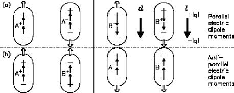
Fig. 1 : Electric dipoles with an electric dipole moment, $d$, each. They can be represented by charges $\pm\,|q|$ and a separation vector, $l$ (explicitly shown for the upper right dipole with a length, $l$ in their rest frame). Parallel spin vectors (small arrows) are introduced for the opposite charges resulting in no magnetic dipole moment. There are two types of dipoles, designated by A and B, each with a positive (A⁺, B⁺) and negative (A^-, B^-) spin with respect to the velocity vectors (open arrows). Various combinations of these bosons are displayed that would represent: (a) classical electrostatic fields on larger scales and (b) no mean electrostatic fields, but in all cases no magnetic fields.

The dipole moment of the postulated particles is

$$\mbox{\boldmath$d$}=|q|\,\mbox{\boldmath$l$}$$ (15)

parallel or antiparallel to the velocity vector, $c_{0}\,\hat{\mbox{\boldmath$n$}}$. This assumption is necessary in order to get attraction and repulsion of charges depending on their mutual polarities. In Sect. 3.5 it will, however, be shown that the value of the dipole moment is not critical. The dipoles have a mean kinetic energy, $\overline{T_{\rm D}^{\infty}}>0$, and a momentum

$$\overline{\mbox{\boldmath$p$}_{\rm D}}=\frac{\overline{T_{\rm D}^{\infty}}}{c_{0}}\,\hat{\mbox{\boldmath$n$}}~{},$$ (16)

where $T_{\rm D}^{\infty}$ represents the energy spectrum of the dipoles. As a working hypothesis, it will first be assumed that $T_{\rm D}\equiv\overline{T_{\rm D}^{\infty}}$ is constant remote from any charges with the same value for all dipoles of an isotropic distribution. The question what determines the energy of a dipole will be left open, but one idea could, however, be that the frequency of a longitudinal oscillation of the charges is of importance. In Sect. 4, it will be necessary to consider the energy spectrum of the dipoles.

3.2 Interactions with charged particles

Next it will be postulated that a particle with charge, $Q$, and mass, $m_{Q}$, is emitting directed dipoles with $\mbox{\boldmath$p$}_{\rm D}$. The emission rate should be proportional to its charge, and the orientation such that a repulsion exists between the charge and the dipoles. The details of the process leading to the ejection cannot be specified at this stage. The far-field aspects will be the main interest here. The propagating dipoles are considered to be real particles and not virtual ones as assumed in the Quantum Field Theory. First a description will, as much as possible, be given along the lines of classical field concepts, although the interpretation is later very different. The conservation of energy and momentum will be taken into account, but neither any quantum electrodynamic aspects nor complications introduced by a particle spin. A mass $m_{Q}$ of the charge $Q$ has explicitly been mentioned, because the massless dipole charges are not assumed to absorb and emit any dipoles themselves. The conservation of momentum could hardly be fulfilled in such a process.

From energy conservation it follows that a charge must be able to absorb dipoles as well. Otherwise it has to be assumed that the emission is powered by a reduction of $m_{Q}$; an option that will be excluded. Therefore, the vacuum is thought to be permeated by dipoles that are, in the absence of near charges, randomly oriented and directed with (almost) no interaction among each other. Note that such dipoles have no mean interaction energy, even in the classical theory (see e. g. Jackson, 2006). Their number density in space be $\rho_{\rm E}=\mathrm{\Delta}N_{\rm E}/\mathrm{\Delta}V$, assumed to be a nearly constant quantity, possibly slowly varying in space and time. Whether this “background dipole radiation” and the “quadrupole radiation” proposed by Wilhelm et al. (2013) to model the gravitational attraction are related to the dark matter and dark energy problems is of no concern here.

A charge, $Q$, absorbs and emits dipoles at a rate

$$\frac{\mathrm{\Delta}N_{Q}}{\mathrm{\Delta}t}=\kappa_{\rm E}\,\rho_{\rm E}\,|Q|=\eta_{\rm E}\,|Q|~{},$$ (17)

where $\eta_{\rm E}$ and $\kappa_{\rm E}$ are the corresponding (electrostatic) emission and absorption coefficients – the latter will, however, be called interaction coefficient, because it controls the interaction rate of a charge with a certain spatial dipole density. The momentum conservation can, in general, be fulfilled by isotropic absorption and emission processes. The assumptions as outlined will lead to a distribution of the emitted dipoles in the rest frame of an isolated charge, $Q$, with a spatial density of

$$\rho_{Q}(r)=\frac{\mathrm{\Delta}N_{Q}}{\mathrm{\Delta}V_{r}}=\frac{1}{4\,\pi\,r^{2}\,c_{0}}\,\frac{\mathrm{\Delta}N_{Q}}{\mathrm{\Delta}t}=\frac{\eta_{\rm E}}{c_{0}}\,\frac{|Q|}{4\,\pi\,r^{2}}~{},$$ (18)

where $\mathrm{\Delta}V_{r}$ is given in Eq. (14). The radial emission is part of the background, which has a larger number density than $\rho_{Q}(r)$ at most distances, $r$, of interest. Note that the emission of the dipoles from $Q$ does not change the number density, $\rho_{\rm E}$, in the environment of the charge, but reverses the orientation of about half of the dipoles affected. Details of the interaction involving virtual dipoles to achieve this orientation are presented in Sect. 3.2 with special reference to Fig. 3.

The total number of dipoles will, of course, not be changed either. For a certain $r_{Q}$, defined as the charge radius of $Q$, it has to be

$$\rho_{\rm E}=\left[\frac{\mathrm{\Delta}N_{Q}}{\mathrm{\Delta}V_{r}}\right]_{r_{Q}}=\frac{\eta_{\rm E}}{c_{0}}\,\frac{|Q|}{4\,\pi\,r^{2}_{Q}}~{},$$ (19)

because all dipoles of the background that come so close interact with the charge $Q$ in some way. At this stage, this is a formal description awaiting further quantum electrodynamic studies in the near-field region of charges. The quantity $\rho_{Q}(r)$ for $r>r_{Q}$ depends on the dipole emission at the time $t_{0}=t_{Q}-r/c_{0}$ in line with the required retardation.

The same arguments apply to a charge $q\neq Q$. Since $\rho_{\rm E}$ cannot depend on either $q$ or $Q$, the quantity

$$\sigma_{\rm E}=\frac{|q|}{4\,\pi\,r^{2}_{q}}=\frac{|Q|}{4\,\pi\,r^{2}_{Q}}=\frac{|e|}{4\,\pi\,r^{2}_{\rm E}}$$ (20)

must be independent of the charge, and can be considered as a kind of surface charge density, cf. “Flächenladung” of an electron defined by Abraham (1902), that is the same for all charged particles. The equation shows that $\sigma_{\rm E}$ is determined by the electron charge radius, $r_{\rm E}$, for which estimates will be provided in Sect. 3.5. From Eqs. (17) to (20) it then follows that

$$\kappa_{\rm E}\,\sigma_{\rm E}=c_{0}~{}.$$ (21)

The directed dipole flux would lead to a polarization of the vacuum with an apparent electric field $\mbox{\boldmath$E$}_{\rm P}$ that can be treated in analogy to the polarization $\mbox{\boldmath$P$}=(\varepsilon-\varepsilon_{0})\,\mbox{\boldmath$E$}$ of matter in the classical theory (cf. e. g. Hund, 1957, p. 60). In the latter case for $\varepsilon\neq\varepsilon_{0}$, the polarization is a consequence of the electric field. In our case, however, the polarization is caused by the emission characteristics of charged particles and can be interpreted as an electric field. Note in this context that the Lorentz transformations do not affect the electric field component in the boost direction. Applying the usual polarization definitions , $\mbox{\boldmath$E$}_{\rm P}$ can be written as

$$\mbox{\boldmath$E$}_{\rm P}(r)=-\frac{\mbox{\boldmath$d$}}{\varepsilon_{0}}\,\frac{\mathrm{\Delta}N_{Q}}{\mathrm{\Delta}V_{r}}$$ (22)

and, with Eqs. (3) and (18), $|\mbox{\boldmath$d$}|=c_{0}/\eta_{\rm E}$.

In such an electric field, $E$, the dipole potential energy would be

$$T_{d}=-\mbox{\boldmath$d$}\cdot\mbox{\boldmath$E$}~{}.$$ (23)

At this point, the question of the energy density of the electric field in Eq. (5) will be taken up again – the example of the plane plate capacitor in Sect. 1. Eq. (22) can be generalized to

$$\mbox{\boldmath$E$}=-\frac{\mbox{\boldmath$d$}}{\varepsilon_{0}}\,\frac{\mathrm{\Delta}N_{\|}}{\mathrm{\Delta}V}~{},$$ (24)

where $\mathrm{\Delta}N_{\|}/\mathrm{\Delta}V$ denotes the density of the aligned dipoles without reference to a central charge. For completeness it should be mentioned that two or more aligned dipole distributions have to be added taking their vector characteristics into account, in the same way as classical electric fields. This also applies, when the distributions of many charges have to be evaluated. The aim of the dipole model is to provide a physical process describing the interaction of charged particles and not to disprove Eqs. (1) to (3). According to Eq. (23), this assembly of dipoles has (in the electric field $E$) the potential energy density

$$w_{\rm P}=-\mbox{\boldmath$d$}\cdot\mbox{\boldmath$E$}\,\frac{\mathrm{\Delta}N_{\|}}{\mathrm{\Delta}V}~{}.$$ (25)

By turning the orientation of half of them around, the electric field would vanish. The energy density of the electric field thus is with Eq. (24)

$$w=\frac{w_{\rm P}}{2}=\frac{\varepsilon_{0}}{2}\,\mbox{\boldmath$E$}^{2}~{}.$$ (26)

The energy density of the field is just a consequence of the dipole distributions and orientations. Outside of the plane plate capacitor discussed in Sect. 1, the orientations are such that they compensate each other, and it is $w=0$.

This description of the relationship between the configuration of the dipole distribution and the electric field suffers from the fact that both the classical electric field and its interaction with electric charges and dipoles do not exist in the new concept. Consequently, the classical equations of charged-particle physics as summarized, for instance, by Rohrlich (1997) cannot be applied, and alternative solutions have to be conceived.

3.3 Virtual dipoles

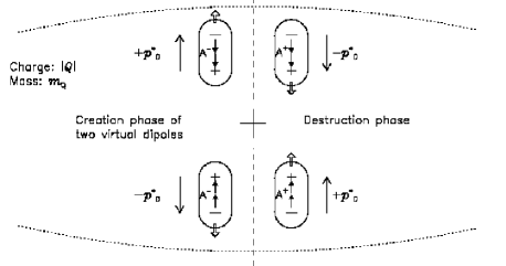
Fig. 2 : Conceptional presentation of the creation and destruction phases of virtual dipole pairs by a charge, and the corresponding momentum vectors of the virtual dipoles.

As a first step, a formal way of achieving the required momentum and energy transfers by discrete interactions will be described: the idea is based on virtual dipoles in analogy to other virtual particles (cf. e. g. v. Weizsäcker, 1934; Yukawa, 1935; Nimtz and Stahlhofen, 2008). The symmetric creation and destruction of virtual dipoles is sketched in Fig. 2. The momentum balance is shown for the emission phase on the left and the absorption phase on the right.

Virtual dipoles with energies of $T^{*}_{\rm D}\ll m_{Q}\,c^{2}_{0}$ supplied by a central body with charge $Q$ and mass $m_{Q}$ will have a certain lifetime $\mathrm{\Delta}t_{\rm E}$ and interact with “real” dipoles. This concept implies that electric point charges do not exist. Any charge has an interaction radius (cf. Eq. 4 for the classical theory). In the literature, there are many different derivations of an energy-time relation (cf. Mandelstam and Tamm, 1945; Aharonov and Bohm, 1961; Hilgevoord, 1998). Considerations of the spread of the frequencies of a limited wave-packet led Bohr (1949) to an approximation for the indeterminacy of the energy that can be re-written as

$$T^{*}_{\rm D}\approx h/\mathrm{\Delta}t_{\rm E}$$ (27)

with $h=6.626\ldots\times 10^{-34}$ J s, the Planck constant. For propagating dipoles, the equation

$$l_{\rm E}=c_{0}\,\mathrm{\Delta}t_{\rm E}=\frac{h}{p_{\rm D}}=\frac{h\,c_{0}}{T_{\rm D}}$$ (28)

is equivalent to the photon energy relation $E_{\nu}=h\,\nu=h\,c_{0}/\lambda$, where $\mathrm{\Delta}t_{\rm E}$ now corresponds to the period and $\lambda$ to $l_{\rm E}$, which can be considered as the de Broglie wavelength of the hypothetical dipoles and their interaction length. The relationship between the interaction length, defined in Eq. (28), and the charge radius in Eq. (20) could not be elucidated in this conceptual study. Since there is, however, experimental evidence that virtual photons (identified as evanescent electromagnetic modes) behave non-locally (Low and Mende, 1991; Stahlhofen and Nimtz, 2006), the virtual dipoles might also behave non-locally and the absorption of a dipole can occur momentarily by the annihilation with an appropriate virtual particle. Eq. (28) would thus not be relevant in this context.

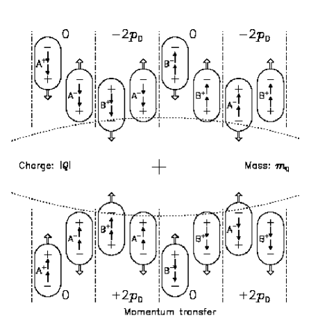
Fig. 3 : Virtual dipoles of a charge $+|Q|$ (with mass $m_{Q}$) interact with “real” dipoles, A⁺ and A^- arriving with a momentum $-\,p_{\rm D}$, each. On the left, a dipole A⁺ annihilates in the lower dashed-dotted box with virtual dipole A⁺ in the destruction phase (cf. Fig. 2) and liberates dipole B⁺. No momentum will be transferred to the central charge with $p_{\rm D}=p^{*}_{\rm D}$. The other type of interaction – called direct interaction, in contrast to the indirect one on the left – also requires two virtual dipoles, one of them annihilates in the creation phase (see again Fig. 2) with dipole A^- (in the upper box with dashed-dotted boundaries), the other one is liberated by the excess energy of the annihilation. The central charge received a momentum of $-(p_{\rm D}+p^{*}_{\rm D})$. No spin reversal has been assumed in both cases.

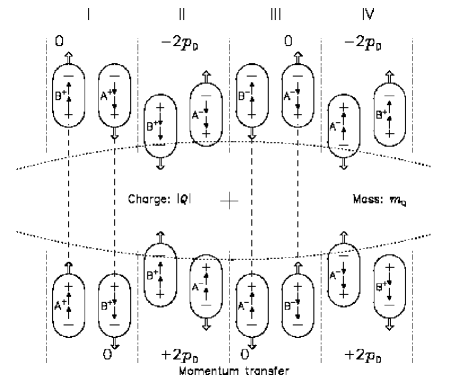
Fig. 4 : Electric dipoles are approaching and leaving a charge $|Q|$ with nearly radial orientations of their dipole moments. The central charge faces equal polarities of the outgoing dipoles. The interaction of the charge with the dipole distribution in an initially chaotic environment generates a configuration with spherical symmetry. Only two directions are shown with groups of incoming and outgoing dipoles in four vertical columns. The interaction region is indicated by dotted lines. (Note that the dipole trajectories are actually converging or diverging. Together they act as an equivalent of a classical inhomogeneous electric field.) By employing the virtual dipole interaction processes shown in Fig. 3 the dipoles A⁺ and B^- arriving from above and below in columns I and III are “transmitted” without transferring momentum to the central charge, but experience a reversal of the dipole moment during an indirect interaction. The dipoles A^- and B⁺ in columns II and IV, however, are “reflected” with momentum transfers as indicated in direct interactions. A downward momentum transfer is reckoned negative. There is no net momentum transfer to the charge in a symmetric configuration.

During a direct interaction, the dipole A^- (in Fig. 3 on the right side) annihilates together with an identical virtual dipole with an opposite velocity vector. This postulate is motivated by the fact that it provides the easiest way to eliminate the charges and yield $P=-\,p_{\rm D}+p^{*}_{\rm D}=0$ (where $p^{*}_{\rm D}$ is the momentum of the virtual dipole) as well as $S=0$ for charges at rest in a system with an isotropic distribution of $\mbox{\boldmath$p$}_{\rm G}$ (cf. Sect. 3.1). The momentum balance is neutral and the excess energy, $T_{\rm D}$, is used to liberate a second virtual dipole B⁺, which has the required orientation. The charge had emitted two virtual dipoles with a momentum of $+\,p^{*}_{\rm D}$, each, and a total momentum of $-(p_{\rm D}+p^{*}_{\rm D})$ was transferred to $|Q|$. The process can be described as a reflection of a dipole together with a reversal of the dipole momentum. The number of these direct interactions will be denoted by $\mathrm{\Delta}\hat{N}_{Q}$. The dipole of type A⁺ (on the left side) can exchange its momentum in an indirect interaction only on the far side of the charge with an identical virtual dipole during its absorption (or destruction) phase (cf. Fig. 2). The excess energy of $T_{\rm D}$ is supplied to liberate a second virtual dipole B⁺. The momentum transfer to the charge $+\,|Q|$ is zero. This process just corresponds to a double charge exchange. Designating the number of interactions of the indirect type with $\mathrm{\Delta}\tilde{N}_{Q}$, it is

$$\frac{\mathrm{\Delta}N_{Q}}{\mathrm{\Delta}t}=\frac{\mathrm{\Delta}\hat{N}_{Q}+\mathrm{\Delta}\tilde{N}_{Q}}{\mathrm{\Delta}t}~{},$$ (29)

with $\mathrm{\Delta}\tilde{N}_{Q}=\mathrm{\Delta}\hat{N}_{Q}=\mathrm{\Delta}N_{Q}/2$. Unless direct and indirect interactions are explicitly specified, both types are meant by the term “interaction”.

In Sect. 4, moving charged bodies will be considered. Since STR requires that a uniform motion is maintained without external forces, it will follow that the absorbed and emitted dipoles must not only have balanced momentum and energy budgets in the rest system of the body, but also in other inertial systems.

The virtual dipole emission rate has to be

$$\frac{\mathrm{\Delta}N^{*}_{Q}}{\mathrm{\Delta}t}=2\,\frac{\mathrm{\Delta}N_{Q}}{\mathrm{\Delta}t}~{},$$ (30)

i.e. the virtual dipole emission rate equals the sum of the real absorption and emission rates. The interaction model described results in a mean momentum transfer per interaction of $p_{\rm D}$ without involving a macroscopic electrostatic field.

A macroscopic dipole encounters in the inhomogeneous dipole distribution of a charge more or less direct or indirect interactions depending on its orientation.

3.4 Coulomb’s law

As a second step, a quantitative evaluation will be considered of the force acting on a test particle with charge, $q$, at a distance, $r$, from another particle with charge $Q$ by the absorption of dipoles not only from the background, but also from the distribution emitted from $Q$ according to Eq. (18) under the assumption of a constant interaction coefficient, $\kappa_{\rm E}$. Both charges are initially at rest in an inertial system, and with large mass-to-charge ratios any accelerations can be neglected. The rate of interchanges between these point sources then is

$$\frac{\mathrm{\Delta}N_{Q,q}}{\mathrm{\Delta}t}=\frac{\eta_{\rm E}\,\kappa_{\rm E}}{c_{0}}\,\frac{|Q|\,|q|}{4\,\pi\,r^{2}}=\frac{\mathrm{\Delta}N_{q,Q}}{\mathrm{\Delta}t}~{},$$ (31)

which confirms the reciprocal relationship between $q$ and $Q$ (after due consideration of the retardation). It should be noted – for later reference – that a relative motion between $q$ and $Q$ will require a relativistic treatment. It is important to realize that all interchange events between pairs of charged particles are either direct or indirect depending on their polarities and transfer a momentum of $2\,p_{\rm G}$ or zero.

In order to get some more insight into the details of the process, a positive test charge, $+\,|q|$, will be positioned below $+\,|Q|$ in Fig. 4. Most of the dipoles arriving from below will still be part of the background, because its density $\rho_{\rm E}$ is much higher than $\rho_{\rm Q}(r)$ for $r\gg r_{\rm Q}$. Assuming that one of them, for instance A⁺ in column I, has been reversed by $+\,|q|$, this will lead to an additional direct interaction and a transfer of $+\,2\,p_{\rm G}$.

The resulting momentum transfer thus becomes positive leading to a repulsion, because the conditions on the opposite side have not changed. The momentum transfer rate from charge  $+\,|q|$ to $+\,|Q|$ thus is with Eq. (31)

$$\left|\frac{\mathrm{\Delta}P_{\rm E}}{\mathrm{\Delta}t}\right|=2\,p_{\rm D}\frac{\mathrm{\Delta}N_{Q,q}}{\mathrm{\Delta}t}~{}.$$ (32)

Conversely, for charges with opposite signs, dipoles emitted from $-\,|q|$ will transfer less momentum to $|Q|$, because more indirect interactions occur. With a reversal of dipole B⁺ in column II, for instance, the balance gets negative with the consequence of an attraction, since there is no compensation for the direct background interactions from the opposite direction. Eq. (32) shows that the choice of the dipole moment is of no importance in this context. With

$$2\,p_{\rm D}\,\frac{\eta_{\rm E}\,\kappa_{\rm E}}{c_{0}}=\frac{1}{\varepsilon_{0}}~{}.$$ (33)

and taking into account the polarities, Eq. (32) becomes

$$K_{\rm E}=\frac{\mathrm{\Delta}P_{\rm E}}{\mathrm{\Delta}t}=\frac{Q\,q}{4\,\pi\,r^{2}\,\varepsilon_{0}}~{},$$ (34)

i.e. Coulomb’s law.

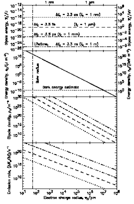
Fig. 5 : Energies of the virtual dipoles according to Eq. (27) are shown as broken lines in the upper panel with the lifetimes, $\mathrm{\Delta}t_{\rm E}$, as parameter (in parentheses, the interaction lengths, $l_{\rm E}$, cf. Eq. 28). In the lower panels, the energy and number densities in space are plotted as well as the emission rates from an elementary charge as functions of the charge radius, $r_{\rm E}$, of a charge $e$ for different $\mathrm{\Delta}t_{\rm E}$ values. The Bohr radius, $a_{0}$, and an estimate of the cosmic dark energy (cf. Beck and Mackey, 2005) are indicated. The charge radius consistent with the latter value is shown as vertical dotted line.

The electrostatic force between charged particles has thus been described by the transfer of momentum through electrostatic dipoles moving with $c_{0}$ and aligned along their propagation direction. The description illustrates a physical mechanism for such a force. In this context, it might be appropriate to note that Coulomb’s interaction energy of two electrons follows from quantum electrodynamics if only the longitudinal electromagnetic waves are taken into account (Fermi, 1932; Bethe and Fermi, 1932), (cf. Dirac, 1951a).

3.5 Dipole energy density

Important questions obviously are related to the energy, $T_{\rm D}$, of the dipoles and, even more, to their energy density in space. Eqs. (16) and (19) to (21) together with Eq. (33) allow the energy density to be expressed by

$$\epsilon_{\rm E}=T_{\rm D}\,\rho_{\rm E}=\frac{\sigma^{2}_{\rm E}}{2\,\varepsilon_{0}}~{}.$$ (35)

This quantity is independent of both the dipole moment and energy. It takes into account all dipoles (whether their distribution is chaotic or not). Should the energy density vary in space and / or time, the surface charge density, $\sigma_{\rm E}$, must vary as well. However, as long as $\kappa_{\rm E}$ and $\eta_{\rm E}$ obey Eqs. (21) and (33), Eq. (32) would be equivalent to Coulomb’s law.

The electric dipole moment is related to the other dipole characteristics discussed so far, only if the definition of an electrostatic field according to Eq. (22) is upheld. Without that requirement, the value of the dipole moment is of no importance and only the polarity remains a salient feature. The other relations are shown in Fig. 5 as function of the charge radius, $r_{\rm E}$, of an electron with the lifetime, $\mathrm{\Delta}t_{\rm E}$, as parameter. If $r_{\rm E}=a_{0}$, the Bohr radius, very high energy densities result and, on the other hand, relatively large $r_{\rm E}$ are required for energy densities in the range of the cosmic dark energy estimates. For the time being, the latter values must be considered as the most likely ones, and it remains to be seen how the charge radius and the interaction length can be further constraint, and whether these relations are consistent with an explicit interaction model.

4 Dipoles and moving particles

Up to now, the interactions of isolated electric charges with dipoles have been treated in an inertial system, in which the charges were assumed to be at rest, but it is, of course, required by STR that any uniformly moving charged particle experiences no deceleration by the background dipole distribution. Since charges are in general not at rest in a single inertial system, such considerations are of great importance. Dirac (1951b) argued that an æther concept could be consistent with STR provided quantum fluctuations of the æther would be taken into account (cf. also Vigier, 1995). In the meantime, experimental results have indicated that virtual particles show a non-local behaviour (Low and Mende, 1991; Stahlhofen and Nimtz, 2006; Nimtz and Stahlhofen, 2008). It, therefore, does not seem to be hopeless to show that charged particles at rest in different inertial systems would be affected in the same way by isotropic dipole distributions. This has, in fact, been shown for moving masses relative to a quadrupole distribution (Wilhelm et al., 2013) and can be directly applied here. The calculations for electric dipoles will give $\mathrm{\Delta}m=0$, because the gravitational energy reduction parameter $Y$ is not relevant in the electrostatic case.

5 Discussion

Some consequences resulting from the concepts developed are discussed in the following sections.

5.1 Outlook

There are several topics that, in principle, should have been treated in this context, but would either require detailed calculations outside the scope of this conceptional presentation, or further far-reaching assumptions. Within the first category fall: (a) forces between parallel conductors and other magnetostatic configurations, considering that many magnetic fields can be transformed into pure electric fields by a change of the inertial system (discussed by Dwivedi et al., 2013); (b) the Aharonov–Bohm effect (Aharonov and Bohm, 1959).

In the second category should be mentioned: (a) the Casimir effect (Casimir, 1949); (b) the dipole and quadrupole energy spectra; (c) the interaction of quadrupoles and dipoles; (d) the contributions of $\epsilon_{\rm E}$ and $\epsilon_{\rm G}$ to the “vacuum energy” density.

6 Conclusion

The electrostatic attraction and repulsion could be described by suitable dipole distributions tailored to emulate Coulomb’s law. This concept allows a formulation of the far-reaching electrostatic force between charged particles as local interactions of postulated electric dipoles travelling with the speed of light in vacuum.

References

- Abraham (1902) Abraham, M.: Prinzipien der Dynamik des Elektrons. Ann. Phys. (Leipzig), 315, 105 (1902)
- Aharonov and Bohm (1959) Aharonov, Y., and Bohm, D.: Significance of electromagnetic potentials in the quantum theory. Phys. Rev., 115, 485 (1959)
- Aharonov and Bohm (1961) Aharonov, Y., and Bohm, D.: Time in the quantum theory and the uncertainty relation for time and energy. Phys. Rev., 122, 1649 (1961)
- Beck and Mackey (2005) Beck, C., and Mackey, M.C.: Could dark energy be measured in the lab? Phys. Lett. B, 605, 295 (2005)
- Bethe and Fermi (1932) Bethe, H., and Fermi, E.: Über die Wechselwirkung von zwei Elektronen. Z. Phys., 77, 296 (1932)
- Bohr (1949) Bohr, N.: Discussions with Einstein on epistemological problems in atomic physics. In Albert Einstein: Philosopher-Scientist, Cambridge University Press, Cambridge (1949)
- Bonnor (1970) Bonnor, W.B.: Charge moving with the speed of light. Nature, 225, 932 (1970)
- Casimir (1949) Casimir, H.B.G.: Sur les forces van der Waals–London. J. Chim. Phys., 46, 407 (1949)
- Compton (1923) Compton, A.H.: A quantum theory of the scattering of X-rays by light elements. Phys. Rev., 21, 483 (1923)
- Dirac (1951a) Dirac, P.A.M.: A new classical theory of electrons. Proc. Roy. Soc. Lond. A, 209, 291 (1951)
- Dirac (1951b) Dirac, P.A.M.: Is there an Æther? Nature, 168, 906 (1951)
- Drude (1897) Drude, P.: Ueber Fernewirkungen. Ann. Phys. (Leipzig), 268, I (1897)
- Dwivedi et al. (2013) Dwivedi, B.N., Wilhelm, H., and Wilhelm, K.,: Magnetostatics and the electric impact model. arXiv1309.7732 (2013); submitted to International Journal of Magnetics and Electromagnetism (2016)
- Einstein (1905) Einstein, A.: Zur Elektrodynamik bewegter Körper. Ann. Phys., (Leipzig), 322, 891 (1905)
- Einstein (1917) Einstein, A.: Zur Quantentheorie der Strahlung. Phys. Z. XVIII, 121 (1917)
- Fermi (1932) Fermi, E.: Quantum theory of radiation. Rev. Mod. Phys., 4, 87 (1932)
- Finkelnburg (1958) Finkelnburg, W.: Einführung in die Atomphysik. 5./6. Aufl., Springer-Verlag, Berlin, Göttingen, Heidelberg (1958)
- Goldhaber and Nieto (1971) Goldhaber, A.S., and Nieto, M.M.: Terrestrial and extraterrestrial limits on the photon mass. Rev. Mod. Phys., 43, 277 (1971)
- Hänsch et al. (2005) Hänsch, T.W., Alnis, J., Fendel, P., Fischer, M., Gohle, C., Herrmann, M., Holzwarth, R., Kolachevsky, N., Udem, Th., and Zimmermann, M.: Precision spectroscopy of hydrogen and femtosecond laser frequency combs. Phil. Trans. R. Soc. A, 363, 2155 (2005)
- Heaviside (1892) Heaviside, O.: On the forces, stresses, and fluxes of energy in the electromagnetic field. Phil. Trans. R. Soc. Lond. A, 183, 423 (1892)
- Hilgevoord (1998) Hilgevoord, J.: The uncertainty principle for energy and time. II. Am J Phys 66, 396 (1998)
- Hund (1957) Hund, F.: Theoretische Physik. Bd. 2, 3. Aufl., B.G. Teubner Verlagsgesellschaft, Stuttgart (1957)
- Jackiw et al. (1992) Jackiw, R., Kabat, D., and Ortiz, M.: Electromagnetic fields of a massless particle and the eikonal. Phys. Lett. B, 277, 148 (1992)
- Jackson (2006) Jackson, J.D.: Klassische Elektrodynamik. 4. Aufl., Walter de Gruyter, Berlin, New York (2006)
- Kosyakov (2008) Kosyakov, B.P.: Massless interacting particles. J. Phys. A: Math. Theor., 41, 465401 (2008)
- Landé (1950) Landé, A.: On advanced and retarded potentials. Phys. Rev., 80, 283 (1950)
- von Laue (1911) von Laue, M.: Das Relativitätsprinzip. Friedr. Vieweg & Sohn, Braunschweig, (1911)
- Levine et al. (1977) Levine, H., Moniz, E.J., and Sharp, D.H.: Motion of extended charges in classical electrodynamics. Am. J. Phys. 45, 75 (1977)
- Levshakov (2004) Levshakov, S.A.: Astrophysical constraints on hypothetical variability of fundamental constants. Lect. Not. Phys., 648, 151 (2004)
- Lewis (1926) Lewis, G.N.: The conservation of photons. Nature, 118, 874 (1926)
- Low and Mende (1991) Low, F.E., and Mende, P.F.: A note on the tunneling time problem. Ann. Phys. (N.Y.), 210, 380 (1991)
- Mandelstam and Tamm (1945) Mandelstam, L.I., and Tamm, I.E.: The uncertainty relation between energy and time in non-relativistic quantum mechanics. J Phys (USSR) 9, 249 (1945)
- Nimtz and Stahlhofen (2008) Nimtz, G., and Stahlhofen, A.A.: Universal tunneling time for all fields. Ann. Phys. (Berlin), 17, 374 (2008)
- Planck (1909) Planck, M.: Zur Theorie der Wärmestrahlung. Ann. Phys. (Leipzig), 336, 758 (1909)
- Poincaré (1900) Poincaré, H.: The theory of Lorentz and the principle of reaction. Arch. Néerl. Sci. Exact. Nat., 5, 252 (1900)
- Rohrlich (1997) Rohrlich, F.: The dynamics of a charged sphere and the electron. Am. J. Phys., 65, 1051 (1997)
- Schwarzschild (1903) Schwarzschild, K.: Zur Elektrodynamik. II. Die elementare elektrodynamische Kraft. Göttinger Nachr., 128, 132 (1903)
- Stahlhofen and Nimtz (2006) Stahlhofen, A.A., and Nimtz, G.: Evanescent modes are virtual photons. Europhys. Lett., 76, 189 (2006)
- Vigier (1995) Vigier, J.-P.: Derivation of inertial forces from the Einstein–de Broglie–Bohm (E.d.B.B.) causal stochastic interpretation of quantum mechanics. Found. Phys., 25, 1461 (1995)
- v. Weizsäcker (1934) v. Weizsäcker, C.F.: Ausstrahlung bei Stößen sehr schneller Elektronen. Z. Phys., 88, 612 (1934)
- Wheeler and Feynman (1949) Wheeler, J.A., and Feynman, R.P.: Classical electrodynamics in terms of direct interparticle action. Rev. Mod. Phys., 21, 425 (1949)
- Wilhelm et al. (2013) Wilhelm, K., Wilhelm, H., and Dwivedi, B.N.: An impact model of Newton’s law of gravitation. Astrophys. Space Sci., 343, 135 (2013)
- Yukawa (1935) Yukawa, H.: On the interaction of elementary particles I. Proc. Phys.-Math. Soc. Japan, 17, 48 (1935)