Sparse Principal Component Analysis via Rotation and Truncation

Abstract

Sparse principal component analysis (sparse PCA) aims at finding a sparse basis to improve the interpretability over the dense basis of PCA, meanwhile the sparse basis should cover the data subspace as much as possible. In contrast to most of existing work which deal with the problem by adding some sparsity penalties on various objectives of PCA, in this paper, we propose a new method SPCArt, whose motivation is to find a rotation matrix and a sparse basis such that the sparse basis approximates the basis of PCA after the rotation. The algorithm of SPCArt consists of three alternating steps: rotate PCA basis, truncate small entries, and update the rotation matrix. Its performance bounds are also given. SPCArt is efficient, with each iteration scaling linearly with the data dimension. It is easy to choose parameters in SPCArt, due to its explicit physical explanations. Besides, we give a unified view to several existing sparse PCA methods and discuss the connection with SPCArt. Some ideas in SPCArt are extended to GPower, a popular sparse PCA algorithm, to overcome its drawback. Experimental results demonstrate that SPCArt achieves the state-of-the-art performance. It also achieves a good tradeoff among various criteria, including sparsity, explained variance, orthogonality, balance of sparsity among loadings, and computational speed.

Keywords: sparse, principal component analysis, rotation, truncation.

1 Introduction

In many research areas, the data we encountered are usually of very high dimensions, for examples, signal processing, machine learning, computer vision, document processing, computer network, and genetics etc. However, almost all data in these areas have much lower intrinsic dimensions. Thus, how to handle these data is a traditional problem.

1.1 PCA

Principal component analysis (PCA) [1] is one of the most popular analysis tools to deal with this situation. Given a set of data, whose mean is removed, PCA approximates the data by representing them in another orthonormal basis, called loading vectors. The coefficients of the data when represented using these loadings are called principal components. They are obtained by projecting the data onto the loadings, i.e. inner products between the loading vectors and the data vector. Usually, the loadings are deemed as a set of ordered vectors, in that the variances of data explained by them are in a decreasing order, e.g. the leading loading points to the maximal-variance direction. If the data lie in a low dimensional subspace, i.e. the distribution mainly varies in a few directions, a few loadings are enough to obtain a good approximation; and the original high-dimensional data now can be represented by the low-dimensional principal components, so dimensionality reduction is achieved.

Commonly, the dimensions of the original data have some physical explanations. For example, in financial or biological applications, each dimension may correspond to a specific asset or gene [2]. However, the loadings obtained by PCA are usually dense, so the principal component, got by inner product, is a mixture of all dimensions, which makes it difficult to interpret. If most of the entries in the loadings are zeros (sparse), each principal component becomes a linear combination of a few non-zero entries. This facilitates the understanding of the physical meaning of the loadings as well as the principal components [1]. Further, the physical interpretation would be clearer if different loadings have different non-zero entries, i.e. corresponding to different dimensions.

1.2 Sparse PCA

Sparse PCA aims at finding a sparse basis to make the result more interpretable [3]. At the same time, the basis is required to represent the data distribution faithfully. Thus, there is a tradeoff between the statistical fidelity and the interpretability.

During the past decade, a variety of methods for sparse PCA have been proposed. Most of them have considered the tradeoff between sparsity and explained variance. However, there are three points that have not received enough attentions yet: the orthogonality between loadings, the balance of sparsity among loadings, and the pitfall of deflation algorithms.

• Orthogonality. PCA loadings are orthogonal. But in pursuing sparse loadings, this property is easy to lose. Orthogonality is desirable in that it indicates the independence of physical meaning of the loadings. When the loadings are sufficiently sparse, orthogonality usually implies non-overlapping of their supports. So under the background of improving the interpretation of PCA, now each loading is associated with distinctive physical variables, so are the principal components. This makes the interpretation much easier. Besides, if the loadings are not an orthogonal basis, the inner products between the data and the loadings that are used to compute the components do not constitute an exact projection. For an extreme example, if two loadings are very close, the two components would be similar too. This is meaningless.

• Balance of sparsity. There should not be any member of the loadings highly dense, particularly those leading ones that take account of most variance, otherwise it is meaningless. We emphasize this point, because quite a few of existing algorithms yield loadings with the leading ones highly dense (close to those of PCA) while the minor ones highly sparse; so sparsity is achieved by the minor ones while variance is explained by the dense ones. This is unreasonable.

• Pitfall of deflation. Existing work can be categorized into two groups: deflation group and block group. To obtain $r$ sparse loadings, the deflation group computes one loading at a time; more are got via removing components that have been computed [4]. This follows traditional PCA. The block group finds all loadings together. Generally, the optimal loadings found when we restrict the subspace to be of dimension $r$ may not overlap with the $r+1$ optimal loadings when the dimension increases to $r+1$ [5]. This problem does not occur for PCA, whose loadings successively maximize the variance, and the loadings found via deflation are always globally optimal for any $r$. But it is not the case for sparse PCA, the deflation method is greedy and cannot find optimal sparse loadings. However, the block group has the potential.

Finally we mention that by deflation the obtained loadings are nearly orthogonal, while the block group usually does not equip with mechanism to ensure the orthogonality.

1.3 Our Method: SPCArt

In this paper, we propose a new approach called SPCArt (Sparse PCA via rotation and truncation). In contrast to most of traditional work which are based on adding some sparsity penalty on the objective of PCA, the motivation of SPCArt is distinctive. SPCArt aims to find a rotation matrix and a sparse basis such that the sparse basis approximates the loadings of PCA after the rotation. The resulting algorithm consists of three alternative steps: rotate PCA loadings, truncate small entries of them, and update the rotation matrix.

SPCArt turns out to resolve or alleviate the previous three points. It has the following merits. (1) It is able to explain as much variance as the PCA loadings, since the sparse basis spans almost the same subspace as the PCA loadings. (2) The new basis is close to orthogonal, since it approximates the rotated PCA loadings. (3) The truncation tends to produce more balanced sparsity, since vectors of the rotated PCA loadings are of equal length. (4) It is not greedy compared with the deflation group, it belongs to the block group.

The contributions of this paper are four-fold: (1) we propose an efficient algorithm SPCArt achieving good performance over a series of criteria, some of which have been overlooked by previous work; (2) we devise various truncation operations for different situations and provide performance analysis; (3) we give a unified view for a series of previous sparse PCA approaches, together with ours; (4) under the unified view, we find the relation between GPower, rSVD, and our method, and extend GPower [6] and rSVD [7] to a new implementation, called rSVD-GP, to overcome their drawbacks–parameter tuning problem and imbalance of sparsity among loadings.

The rest of the paper is organized as follows: Section 2 introduces representative work on sparse PCA. Section 3 presents our method SPCArt and four types of truncation operations, and analyzes their performance. Section 4 gives a unified view for a series of previous work. Section 5 shows the relation between GPower, rSVD, and our method, and extends GPower and rSVD to a new implementation, called rSVD-GP. Experimental results are provided in Section 6. Finally, we conclude this paper in Section 7.

Table 1: Time complexities for computing $r$ loadings from $n$ samples of dimension $p$. $m$ is the number of iterations. $k$ is the cardinality of a loading. The preprocessing and initialization overheads are omitted. ST and SPCArt have the additional cost of PCA. The complexities of SPCArt listed below are of the truncation types T-$\ell_{0}$ and T-$\ell_{1}$. Those of T-sp and T-en are $O(rp\log p+r^{2}p+r^{3})$.

	PCA [1]	ST [8]	SPCA [9]	PathSPCA [2]	ALSPCA [10]	GPower [6], rSVD-GP, TPower [11]	GPowerB [6], rSVD-GPB	SPCArt
$n>p$	$O(np^{2})$	$O(rp)$	$mO(r^{2}p+rp^{3})$	$O(rkp^{2}+rk^{3})$	$mO(rp^{2})$	$mO(rp^{2})$	$mO(rpn+r^{2}n)$	$mO(r^{2}p+r^{3})$
$n<p$	$O(pn^{2})$	$O(rp)$	$mO(r^{2}p+rnp)$	$O(rknp+rk^{3})$	$mO(rnp)$	$mO(rnp)$	$mO(rpn+r^{2}n)$	$mO(r^{2}p+r^{3})$

2 Related Work

Various sparse PCA methods have been proposed during the past decade. We give a brief review below.

1. Post-processing PCA. In early days, interpretability is gained via post-processing the PCA loadings. Loading rotation (LR) [5] applies various criteria to rotate the PCA loadings so that ’simple structure’ emerges, e.g. varimax criterion drives the entries to be either small or large, which is close to a sparse structure. Simple thresholding (ST) [8] instead obtains sparse loadings via directly setting the entries of PCA loadings below a small threshold to zero.

2. Covariance matrix maximization. More recently, systematic approaches based on solving explicit objectives were proposed, starting from SCoTLASS [3] which optimizes the classical objective of PCA, i.e. maximizing the quadratic form of covariance matrix, while additionally imposing a sparsity constraint on each loading.

3. Matrix approximation. SPCA [9] formulates the problem as a regression-type optimization, so as to facilitate the use of LASSO [12] or elastic-net [13] techniques to solve the problem. rSVD [7] and SPC [14] obtain sparse loadings by solving a sequence of rank-1 matrix approximations, with sparsity penalty or constraint imposed.

4. Semidefinite convex relaxation. Most of the methods proposed so far are local ones, which suffer from getting trapped in local minima. DSPCA [15] transforms the problem into a semidefinite convex relaxation problem, thus global optimality of solution is guaranteed. This distinguishes it from most of the other local methods. Unfortunately, its computational complexity is as high as $O(p^{4}\sqrt{\log p})$ ($p$ is the number of variables), which is expensive for most applications. Later, a variable elimination method [16] of complexity $O(p^{3})$ was developed in order to make the application on large scale problem feasible.

5. Greedy methods. In [17], greedy search and branch-and-bound methods are used to solve small instances of the problem exactly. Each step of the algorithm has a complexity $O(p^{3})$, leading to a total complexity of $O(p^{4})$ for a full set of solutions (solutions of cardinality ranging from 1 to $p$). Later, this bound is improved in the classification setting [18]. In another way, a greedy algorithm PathSPCA [2] was presented to further approximate the solution process of [17], resulting in a complexity of $O(p^{3})$ for a full set of solutions. For a review of DSPCA, PathSPCA, and their applications, see [19].

6. Power methods. The GPower method [6] formulates the problem as maximization of a convex objective function and the solution is obtained by generalizing the power method [20] that is used to compute the PCA loadings. Recently, a new power method TPower [11], and a somewhat different but related power method ITSPCA [21] that aims at recovering sparse principal subspace, were proposed.

7. Augmented lagrangian optimization. ALSPCA [10] solves the problem based on an augmented lagrangian optimization. The most special feature of ALSPCA is that it simultaneously considers the explained variance, orthogonality, and correlation among principal components.

Among them only LR [5], SCoTLASS [3], ALSPCA [10] have considered the orthogonality of loadings. SCoTLASS, rSVD [7], SPC [14], the greedy methods [17, 2], one version of GPower [6], and TPower [11] belong to the deflation group. Only DSPCA’s solution [15] is ensured to be globally optimal.

The computational complexities of some of the above algorithms are summarized in Table 1.

3 SPCArt: Sparse PCA via Rotation and Truncation

We first give a brief overview of SPCArt, next introduce the motivation, and then the objective and optimization, and then the truncation types, and finally provide performance analysis.

The idea of SPCArt is simple. Since any rotation of the $r$ PCA loadings $[V_{1},\dots,V_{r}]\in\mathbb{R}^{p\times r}$ constitutes an orthogonal basis spanning the same subspace, $X=VR$ ($R\in\mathbb{R}^{r\times r}$, $R^{T}R=I$), we want to find a rotation matrix $R$ through which $V$ is transformed to a sparsest basis $X$. It is difficult to solve this problem directly, so instead we would find a rotation matrix and a sparse basis such that the sparse basis approximates the PCA loadings after the rotation $V\approx XR$.

The major notations used are listed in Table 2.

Table 2: Major notations.

notation	interpretation
$A\in\mathbb{R}^{n\times p}$	data matrix with $n$ samples of $p$ variables
$V=[V_{1},V_{2},\dots]$	PCA loadings arranged column-wise. $V_{i}$ denotes the $i$th column. $V_{1:r}$ denotes the first $r$ columns
$R$	rotation matrix
$Z$	rotated PCA loadings, i.e. $VR^{T}$
$X$	spare loadings arranged column-wise, similar to $V$
$Polar(\cdot)$	for a matrix $B\in\mathbb{R}^{n\times p}$, $n\geq p$, let the thin SVD be $WDQ^{T}$, $D\in\mathbb{R}^{p\times p}$, then $Polar(B)=WQ^{T}$
$S_{\lambda}(\cdot)$	$0\leq\lambda<1$. For a vector $x$, $S_{\lambda}(x)$ is entry-wise soft thresholding: $S_{\lambda}(x_{i})=sign(x_{i})(|x_{i}|-\lambda)_{+}$, where $[y]_{+}=y$ if $y\geq 0$ and $[y]_{+}=0$ otherwise
$H_{\lambda}(\cdot)$	$0\leq\lambda<1$. For a vector $x$, $H_{\lambda}(x)$ is entry-wise hard thresholding: $H_{\lambda}(x_{i})=x_{i}[sign(|x_{i}|-\lambda)]_{+}$, i.e. $H_{\lambda}(x_{i})=0$ if $|x_{i}|\leq\lambda$, $H_{\lambda}(x_{i})=x_{i}$ otherwise
$P_{\lambda}(\cdot)$	$\lambda\in\{0,1,2,\cdots\}$. For a vector $x$, $P_{\lambda}(x)$ sets the smallest $\lambda$ entries (absolute value) to be zero
$E_{\lambda}(\cdot)$	$0\leq\lambda<1$. For a vector $x$, $E_{\lambda}(x)$ sets the smallest $k$ entries, whose energy take up at most $\lambda$, to be zero. $k$ is found as following: sort $|x_{1}|,|x_{2}|,\dots$ in ascending order to be $\bar{x}_{1},\bar{x}_{2},\dots$, $k=\max_{i}i,\,s.t.\sum_{j=1}^{i}\bar{x}_{j}^{2}/\|x\|_{2}^{2}\leq\lambda$

3.1 Motivation

Our method is motivated by the solution of the Eckart-Young theorem [22]. This theorem considers the problem of approximating a matrix by the product of two low-rank ones.

Theorem 1.

(Eckart-Young Theorem) Assume the SVD of a matrix $A\in\mathbb{R}^{n\times p}$ is $A=U\Sigma V^{T}$, in which $U\in\mathbb{R}^{n\times m}$, $m\leq min\{n,p\}$, $\Sigma\in\mathbb{R}^{m\times m}$ is diagonal with $\Sigma_{11}\geq\Sigma_{22}\geq\cdots\geq\Sigma_{mm}$, and $V\in\mathbb{R}^{p\times m}$. A rank $r$ ($r\leq m$) approximation of $A$ is to solve the following problem:

$$\min_{Y,X}\|A-YX^{T}\|^{2}_{F},\;s.t.\,X^{T}X=I,$$ (1)

where $Y\in\mathbb{R}^{n\times r}$ and $X\in\mathbb{R}^{p\times r}$. A solution is

$$X^{*}=V_{1:r},\;Y^{*}=AX^{*},$$ (2)

where $V_{1:r}$ is the first $r$ columns of $V$.

Alternatively, the solution can be expressed as

$$Y^{*}=U_{1:r}\Sigma_{1:r},\;X^{*}=Polar(A^{T}Y^{*}),$$ (3)

where $Polar(\cdot)$ is the orthonormal component of the polar decomposition of a matrix [6]. From the more familiar SVD perspective, its equivalent definition is provided in Table 2.

Note that if the row vectors of $A$ have been centered to have mean zero, $V_{1:r}$ are the loadings obtained by PCA. Clearly, $\forall R\in\mathbb{R}^{r\times r}$ and $R^{T}R=I$, $X^{*}=V_{1:r}R$ and $Y^{*}=AX^{*}=U_{1:r}\Sigma_{1:r}R$ is also a solution of (1). This implies that any rotation of the $r$ orthonormal leading eigenvectors $V_{1:r}\in\mathbb{R}^{p\times r}$ is a solution of the best rank $r$ approximation of $A$. That is, any orthonormal basis in the corresponding eigen-subspace is capable of representing the original data distribution as well as the original basis. Thus, a natural idea for sparse PCA is to find a rotation matrix $R$ so that $X=V_{1:r}R$ becomes sparse, i.e.,

$$\min_{R\in\mathbb{R}^{r\times r}}\|V_{1:r}R\|_{0},\;s.t.\;R^{T}R=I,$$ (4)

where $\|\cdot\|_{0}$ denotes the sum of $\ell_{0}$ (pseudo) norm of the columns of a matrix, i.e. it counts the non-zeros of a matrix.

3.2 Objective and optimization

Unfortunately, the above problem is hard to solve. So we approximate it instead. Since $X=V_{1:r}R\Leftrightarrow V_{1:r}=XR^{T}$, we want to find a rotation matrix $R$ through which a sparse basis $X$ approximates the original PCA loadings. Without confusion, we use $V$ to denote $V_{1:r}$ hereafter. For simplicity, the $\ell_{0}$ version will be postponed to next section, we consider the $\ell_{1}$ version first:

$$\begin{split}&\min_{X,R}\;\frac{1}{2}\|V-XR\|^{2}_{F}+\lambda\sum_{i}\|X_{i}\|_{1},\,\\ &s.t.\,\forall i,\,\|X_{i}\|_{2}=1,\,R^{T}R=I.\end{split}$$ (5)

$\|\cdot\|_{1}$ is the $\ell_{1}$ norm of a vector, i.e. sum of absolute values. It is well-known that $\ell_{1}$ norm is sparsity inducing, which is a convex surrogate of the $\ell_{0}$ norm [23]. Under this objective, the solution may not be orthogonal, and may deviate from the eigen-subspace spanned by $V$. However, if the approximation is accurate enough, i.e., $V\approx XR$, then $X\approx VR^{T}$ would be nearly orthogonal and explain similar variance as $V$. Note that the above objective turns out to be a matrix approximation problem as Eckart-Young theorem. The key difference is that sparsity penalty is added. But the solutions still share some common features.

There is no closed-form solutions for $R$ and $X$ simultaneously. We can solve the problem by fixing one and optimizing the other alternately. Both subproblems have closed-form solutions.

3.2.1 Fix $X$, solve $R$

When $X$ is fixed, it becomes a Procrustes problem [9]:

$$\min_{R}\|V-XR\|^{2}_{F},\;s.t.\,R^{T}R=I.$$ (6)

$R^{*}=Polar(X^{T}V)$. It has the same form as the right of (3).

3.2.2 Fix $R$, solve $X$

When $R$ is fixed, it becomes

$$\min_{X}\frac{1}{2}\|VR^{T}-X\|^{2}_{F}+\lambda\sum_{i}\|X_{i}\|_{1},\,s.t.\,\forall i,\,\|X_{i}\|_{2}=1.$$ (7)

There are $r$ independent subproblems, one for each column: $\min_{X_{i}}1/2\|Z_{i}-X_{i}\|^{2}_{2}+\lambda\|X_{i}\|_{1},\,s.t.\,\|X_{i}\|_{2}=1$, where $Z=VR^{T}$. It is equivalent to $\max_{X_{i}}\;Z_{i}^{T}X_{i}-\lambda\|X_{i}\|_{1},\,s.t.\,\|X_{i}\|_{2}=1$. The solution is $X_{i}^{*}=S_{\lambda}(Z_{i})/\|S_{\lambda}(Z_{i})\|_{2}$ [6]. $S_{\lambda}(\cdot)$ is entry-wise soft thresholding, defined in Table 2. This is truncation type T-$\ell_{1}$: soft thresholding.

It has the following physical explanations. $Z$ is rotated PCA loadings, it is orthonormal. $X$ is obtained via truncating small entries of $Z$. On one hand, because of the unit length of each column in $Z$, a single threshold $0\leq\lambda<1$ is feasible to make the sparsity distribute evenly among the columns in $X$; otherwise we have to apply different thresholds for different columns which are hard to determine. On the other hand, because of the orthogonality of $Z$ and small truncations, $X$ is still possible to be nearly orthogonal. These are the most distinctive features of SPCArt. They enable easy analysis and parameter setting.

The algorithm of SPCArt is presented in Algorithm 1, where the truncation in line 7 can be any type, including T-$\ell_{1}$ and the others that will be introduced in next section.

The computational complexity of SPCArt is shown in Table 1. Except the computational cost of PCA loadings, SPCArt scales linearly about data dimension. When the number of loadings is not too large, it is efficient.

Algorithm 1 SPCArt

1:  Input: data matrix $A\in\mathbb{R}^{n\times p}$, number of loadings $r$, truncation type $T$, truncation parameter $\lambda$.

2:  Output: sparse loadings $X=[X_{1},\dots,X_{r}]\in\mathbb{R}^{p\times r}$.

3:  PCA: compute rank-$r$ SVD of $A$: $U\Sigma V^{T}$, $V\in\mathbb{R}^{p\times r}$.

4:  Initialize $R$: $R=I$.

5:  repeat

6:     Rotation: $Z=VR^{T}$.

7:     Truncation: $\forall{i}$, $X_{i}=T_{\lambda}(Z_{i})/\|T_{\lambda}(Z_{i})\|_{2}$.

8:     Update $R$: thin SVD of $X^{T}V$: $WDQ^{T}$, $R=WQ^{T}$.

9:  until convergence

3.3 Truncation Types

In this section, given rotated PCA loadings $Z$, we introduce the truncation operation $T_{\lambda}(Z_{i})$, where $T_{\lambda}$ is any of the following four types: T-$\ell_{1}$ soft thresholding $S_{\lambda}$, T-$\ell_{0}$ hard thresholding $H_{\lambda}$, T-sp truncation by sparsity $P_{\lambda}$, and T-en truncation by energy $E_{\lambda}$. T-$\ell_{1}$ has been introduced in last section, which is resulted from $\ell_{1}$ penalty.

T-$\ell_{0}$: hard thresholding. Set the entries below threshold $\lambda$ to be zero: $X_{i}^{*}=H_{\lambda}(Z_{i})/\|H_{\lambda}(Z_{i})\|_{2}$. $H_{\lambda}(\cdot)$ is defined in Table 2. It is resulted from $\ell_{0}$ penalty:

$$\min_{X,R}\|V-XR\|^{2}_{F}+\lambda^{2}\sum_{i}\|X_{i}\|_{0},\,s.t.\,R^{T}R=I,$$ (8)

The optimization is similar to the $\ell_{1}$ case. Fixing $X$, $R^{*}=Polar(X^{T}V)$. Fixing $R$, the problem becomes $\min_{X}\|VR^{T}-X\|^{2}_{F}+\lambda^{2}\|X\|_{0}$. Let $Z=VR^{T}$, it can be decomposed to $p\times r$ entry-wise subproblems, and the solution is apparent: if $|Z_{ji}|\leq\lambda$, then $X_{ji}^{*}=0$, otherwise $X_{ji}^{*}=Z_{ji}$. Hence the solution can be expressed as $X_{i}^{*}=H_{\lambda}(Z_{i})$.

There is no normalization for $X^{*}$ compared with the $\ell_{1}$ case. This is because if unit length constraint $\|X_{i}\|_{2}=1$ is added, there will be no closed form solution. However, in practice, we still let $X_{i}^{*}=H_{\lambda}(Z_{i})/\|H_{\lambda}(Z_{i})\|_{2}$ for consistency, since empirically no significant difference is observed.

Note that both $\ell_{0}$ and $\ell_{1}$ penalties only result in thresholding operation on $Z$ and nothing else (only make line 7 of Algorithm 1 different). Hence, we may devise other heuristic truncation types irrespective of explicit objective:

T-sp: truncation by sparsity. Truncate the smallest $\lambda$ entries: $X_{i}=P_{\lambda}(Z_{i})/\|P_{\lambda}(Z_{i})\|_{2}$, $\lambda\in\{0,1,\dots,p-1\}$. Table 2 gives the precise definition of $P_{\lambda}(\cdot)$. It can be shown that this heuristic type is resulted from the $\ell_{0}$ constraint:

$$\begin{split}&\min_{X,R}\;\|V-XR\|^{2}_{F},\\ &s.t.\,\forall i,\,\|X_{i}\|_{0}\leq p-\lambda,\;\|X_{i}\|_{2}=1,\,R^{T}R=I.\end{split}$$ (9)

When $X$ is fixed, the solution is the same as $\ell_{0}$ and $\ell_{1}$ cases above. When $R$ is fixed, the solution is $X_{i}^{*}=P_{\lambda}(Z_{i})/\|P_{\lambda}(Z_{i})\|_{2}$, where $Z=VR^{T}$. The proof is put in Appendix A.

T-en: truncation by energy. Truncate the smallest entries whose energy (sum of square) take up $\lambda$ percentage: $X_{i}=E_{\lambda}(Z_{i})/\|E_{\lambda}(Z_{i})\|_{2}$. $E_{\lambda}$ is described in Table 2. However, we are not aware of any objective associated with this type.

Algorithm 1 describes the complete algorithm of SPCArt with any truncation type.

SPCArt promotes the seminal ideas of simple thresholding [8] and loading rotation [5]. When using T-$\ell_{0}$, the first iteration of SPCArt, i.e. $X_{i}=H_{\lambda}(V_{i})$, corresponds to the ad-hoc simple thresholding ST, which is frequently used in practice and sometimes produced good results [9, 17]. In another way, the motivation of SPCArt, i.e. (4), is similar to the loading rotation, whereas SPCArt explicitly seeks sparse loadings via $\ell_{0}$ pseudo-norm, loading rotation seeks ’simple structure’ via various criteria, e.g. the varimax criterion, which maximizes the variances of squared loadings $\sum_{i}[\sum_{j}Z_{ji}^{4}-1/p(\sum_{k}Z_{ki}^{2})]$, where $Z=VR$, drives the entries to distribute unevenly, either small or large (see Section 7.2 in [1]).

3.4 Performance Analysis

This section discusses the performance bounds of SPCArt with each truncation type. For $X_{i}=T_{\lambda}(Z_{i})/\|T_{\lambda}(Z_{i})\|_{2}$, $i=1,\dots,r$, we study the following problems:

(1) How much sparsity of $X_{i}$ is guaranteed?

(2) How much $X_{i}$ deviates from $Z_{i}$?

(3) How is the orthogonality of $X$?

(4) How much variance is explained by $X$?

The performance bounds derived are functions of $\lambda$. Thus, we can directly or indirectly control sparsity, orthogonality, and explained variance via $\lambda$. We give some definitions first.

Definition 2.

$\forall x\in\mathbb{R}^{p}$, the sparsity of $x$ is the proportion of zero entries: $s(x)=1-\|x\|_{0}/p.$

Definition 3.

$\forall z\in\mathbb{R}^{p}$, $z\neq 0$, $x=T_{\lambda}(z)/\|T_{\lambda}(z)\|_{2}$, the deviation of $x$ from $z$ is $\sin(\theta(x,z))$, where $\theta(x,z)$ is the included angle between $x$ and $z$, $0\leq\theta(x,z)\leq\pi/2$. If $x=0$, $\theta(x,y)$ is defined to be $\pi/2$.

Definition 4.

$\forall x,\,y\in\mathbb{R}^{p}$, $x\neq 0$, $y\neq 0$, the nonorthogonality between $x$ and $y$ is $|\cos(\theta(x,y))|=|x^{T}y|/(\|x\|_{2}\cdot\|y\|_{2})$, where $\theta(x,y)$ is the included angle between $x$ and $y$.

Definition 5.

Given data matrix $A\in\mathbb{R}^{n\times p}$ containing $n$ samples of dimension $p$, $\forall$ basis $X\in\mathbb{R}^{p\times r}$, $r\leq p$, the explained variance of $X$ is $EV(X)=tr(X^{T}A^{T}AX)$. Let $U$ be any orthonormal basis in the subspace spanned by $X$, then the cumulative percentage of explained variance is $CPEV(X)=tr(U^{T}A^{T}AU)/tr(A^{T}A)$ [7].

Intuitively, larger $\lambda$ leads to higher sparsity and larger deviation. When two truncated vectors deviate from their originally orthogonal vectors, in the worst case, the nonorthogonality of them degenerates as the ‘sum’ of their deviations. In another way, if the deviations of a sparse basis from the rotated loadings are small, we expect the sparse basis still represents the data well, and the explained variance or cumulative percentage of explained variance maintains similar level to that of PCA. So, both the nonorthogonality and the explained variance depend on the deviations, and the deviation and sparsity in turn are controlled by $\lambda$. We now go into details. The proofs of some of the following results are included in Appendix B.

3.4.1 Orthogonality

Proposition 6.

The relative upper bound of nonorthogonality between $X_{i}$ and $X_{j}$, $i\neq j$, is

$$|\cos(\theta(X_{i},X_{j}))|\leq$$ (10)

$$\begin{cases}\sin(\theta(X_{i},Z_{i})+\theta(X_{j},Z_{j}))&,\theta(X_{i},Z_{i})+\theta(X_{j},Z_{j})\leq\frac{\pi}{2},\\ 1&,\text{otherwise.}\end{cases}$$

The bounds can be obtained by considering the two conical surfaces generated by axes $Z_{i}$ with rotational angles $\theta(X_{i},Z_{i})$. The proposition implies the nonorthogonality is determined by the sum of deviated angles. When the deviations are small, the orthogonality is good. The deviation depends on $\lambda$, which is analyzed below.

3.4.2 Sparsity and Deviation

The following results only concern a single vector of the basis. We will denote $Z_{i}$ by $z$, and $X_{i}$ by $x$ for simplicity, and derive bounds of sparsity $s(x)$ and deviation $\sin(\theta(x,z))$ for each $T$. They depend on a key value $1/\sqrt{p}$, which is the entry value of a uniform vector.

Proposition 7.

For T-$\ell_{0}$, the sparsity bounds are

$$\begin{cases}0\leq s(x)\leq 1-\frac{1}{p}&\text{, $\lambda<\frac{1}{\sqrt{p}}$,}\\ 1-\frac{1}{p\lambda^{2}}<s(x)\leq 1&\text{, $\lambda\geq\frac{1}{\sqrt{p}}$.}\end{cases}$$ (11)

Deviation $\sin(\theta(x,z))=\|\bar{z}\|_{2}$, where $\bar{z}$ is the truncated part: $\bar{z}_{i}=z_{i}$ if $x_{i}=0$, and $\bar{z}_{i}=0$ otherwise. The absolute bounds are:

$$0\leq\sin(\theta(x,z))\leq\begin{cases}\sqrt{p-1}\lambda&\text{, $\lambda<\frac{1}{\sqrt{p}}$,}\\ 1&\text{, $\lambda\geq\frac{1}{\sqrt{p}}$.}\end{cases}$$ (12)

All the above bounds are achievable.

Because when $\lambda<1/\sqrt{p}$, there is no sparsity guarantee, $\lambda$ is usually set to be $1/\sqrt{p}$ in practice. Generally it works well.

Proposition 8.

For T-$\ell_{1}$, the bounds of $s(x)$ and lower bound of $\sin(\theta(x,z))$ are the same as T-$\ell_{0}$. In addition, there are relative deviation bounds

$$\|\bar{z}\|_{2}\leq\sin(\theta(x,z))<\sqrt{\|\bar{z}\|^{2}_{2}+\lambda^{2}\|x\|_{0}}.$$ (13)

It is still an open question that whether T-$\ell_{1}$ has the same upper bound of $\sin(\theta(x,z))$ as T-$\ell_{0}$. By the relative lower bounds, we have

Corollary 9.

The deviation due to soft thresholding is always larger than that of hard thresholding, if the same $\lambda$ is applied.

This implies that results got by T-$\ell_{1}$ have potentially greater sparsity and less explained variance than those of T-$\ell_{0}$.

Proposition 10.

For T-sp, $\lambda/p\leq s(z)<1$, and

$$0\leq\sin(\theta(x,z))\leq\sqrt{\lambda/p}\;.$$ (14)

Except the unusual case that $x$ has many zeros, $s(z)=\lambda/p$. The main advantage of T-sp lies in its direct control on sparsity. If specific sparsity is wanted, it can be applied.

Proposition 11.

For T-en, $0\leq\sin(\theta(x,z))\leq\sqrt{\lambda}$. In addition

$$\lfloor{\lambda p}\rfloor/p\leq s(x)\leq 1-1/p.$$ (15)

If $\lambda<1/p$, there is no sparsity guarantee. When $p$ is moderately large, $\lfloor{\lambda p}\rfloor/p\approx\lambda$.

Due to the discrete nature of operand, the actually truncated energy can be less than $\lambda$. But in practice, especially when $p$ is moderately large, the effect is negligible. So we usually have $\sin(\theta(x,z))\approx\sqrt{\lambda}$. The main advantage of T-en is that it has direct control on deviation. Recall that the deviation has direct influence on the explained variance. Thus, if it is desirable to gain specific explained variance, T-en is preferable. Besides, if $p$ is moderately large, T-en also gives nice control on sparsity.

3.4.3 Explained Variance

Finally, we derive bounds on the explained variance $EV(X)$. Two results are provided. The first one is general and is applicable to any basis $X$ not limited to sparse ones. The second one is tailored to SPCArt.

Theorem 12.

Let rank-$r$ SVD of $A\in\mathbb{R}^{n\times p}$ be $U\Sigma V^{T}$, $\Sigma\in\mathbb{R}^{r\times r}$. Given $X\in\mathbb{R}^{p\times r}$, assume SVD of $X^{T}V$ is $WDQ^{T}$, $D\in\mathbb{R}^{r\times r}$, $d_{min}=\min_{i}D_{ii}$. Then

$$d_{min}^{2}\cdot EV(V)\leq EV(X),$$ (16)

and $EV(V)=\sum_{i}\Sigma^{2}_{ii}$.

The theorem can be interpreted as follows. If $X$ is a basis that approximates rotated PCA loadings well, then $d_{min}$ will be close to one, and so the variance explained by $X$ is close to that explained by PCA. Note that variance explained by PCA loadings is the largest value that is possible to be achieved by orthonormal basis. Conversely, if $X$ deviates much from the rotated PCA loadings, then $d_{min}$ tends to zero, so the variance explained by $X$ is not guaranteed to be much. We see that the less the sparse loadings deviates from rotated PCA loadings, the more variance they explain.

When SPCArt converges, i.e. $X_{i}=T_{\lambda}(Z_{i})/\|T_{\lambda}(Z_{i})\|_{2}$, $Z=VR^{T}$, and $R=Polar(X^{T}V)$ hold simultaneously, we have another estimation. It is mainly valid for T-en.

Theorem 13.

Let $C=Z^{T}X$, i.e. $C_{ij}=\cos(\theta(Z_{i},X_{j}))$, and let $\bar{C}$ be $C$ with diagonal elements removed. Assume $\theta(Z_{i},X_{i})=\theta$ and $\sum^{r}_{j}C_{ij}^{2}\leq 1$, $\forall i$, then

$$(\cos^{2}(\theta)-\sqrt{r-1}\sin(2\theta))\cdot EV(V)\leq EV(X).$$ (17)

When $\theta$ is sufficiently small,

$$(\cos^{2}(\theta)-O(\theta))\cdot EV(V)\leq EV(X).$$ (18)

Since the sparse loadings are obtained by truncating small entries of the rotated PCA loadings, and $\theta$ is the deviation angle between these sparse loadings and the rotated PCA loadings, the theorem implies, if the deviation is small then the variance explained by the sparse loadings is close to that of PCA, as $\cos^{2}(\theta)\approx 1$. For example, if the truncated energy $\|\bar{z}\|^{2}_{2}=\sin^{2}(\theta)$ is about 0.05, then 95% EV of PCA loadings is guaranteed.

The assumptions $\theta(Z_{i},X_{i})=\theta$ and $\sum^{r}_{j}C_{ij}^{2}\leq 1$, $\forall i$, are roughly satisfied by T-en using small $\lambda$. Uniform deviation $\theta(Z_{i},X_{i})=\theta$, $\forall i$, can be achieved by T-en as indicated by Proposition 11. $\sum^{r}_{j}C_{ij}^{2}\leq 1$ means the sum of projected length is less than 1, when $Z_{i}$ is projected onto each $X_{j}$. It must be satisfied if $X$ is exactly orthogonal, whereas it is likely to be satisfied if $X$ is nearly orthogonal (note $Z_{i}$ may not lie in the subspace spanned by $X$), which can be achieved by setting small $\lambda$ according to Proposition 6. In this case, about $(1-\lambda)EV(V)$ is guaranteed.

In practice, we prefer CPEV [7] to EV. CPEV measures the variance explained by subspace rather than basis. Since it is also the projected length of $A$ onto the subspace spanned by $X$, the higher CPEV is, the better $X$ represents the data. If $X$ is not an orthogonal basis, EV may overestimates or underestimates the variance. However, if $X$ is nearly orthogonal, the difference is small, and it is nearly proportional to CPEV.

4 A Unified View to Some Prior Work

A series of methods: PCA [1], SCoTLASS [3], SPCA [9], GPower [6], rSVD [7], TPower [11], SPC [14], and SPCArt, though proposed independently and formulated in various forms, can be derived from the common source of Theorem 1, the Eckart-Young Theorem. Most of them can be seen as the problems of matrix approximation (1), with different sparsity penalties. Most of them have two matrix variables, and the solutions of them usually can be obtained by an alternating scheme: fix one and solve the other. Similar to SPCArt, the two subproblems are a sparsity penalized/constrained regression problem and a Procrustes problem.

PCA [1]. Since $Y^{*}=AX^{*}$, substituting $Y=AX$ into (1) and optimizing $X$, the problem is equivalent to

$$\max_{X}tr(X^{T}A^{T}AX),\;s.t.\,X^{T}X=I.$$ (19)

The solution is provided by Ky Fan theorem [24]: $X^{*}=V_{1:r}R$, $\forall R^{T}R=I$. If $A$ has been centered to have mean zero, the special solution $X^{*}=V_{1:r}$ are exactly the $r$ loadings obtained by PCA.

SCoTLASS [3]. Constraining $X$ to be sparse in (19), we get SCotLASS

$$\max_{X}tr(X^{T}A^{T}AX),\,s.t.\,X^{T}X=I,\,\forall i,\,\|X_{i}\|_{1}\leq\lambda.$$ (20)

However, the problem is not easy to solve.

SPCA [9]. If we substitute $Y=AX$ into (1) and separate the two $X$’s into two independent variables $X$ and $Z$ (so as to solve the problem via alternating), and then impose some penalties on $Z$, we get SPCA

$$\begin{split}&\min_{Z,\,X}\;\|A-AZX^{T}\|^{2}_{F}+\lambda\|Z\|^{2}_{F}+\sum_{i}\lambda_{1i}\|Z_{i}\|_{1},\,\\ &s.t.\,X^{T}X=I,\end{split}$$ (21)

where $Z$ is treated as target sparse loadings and $\lambda$’s are weights. When $X$ is fixed, the problem is equivalent to $r$ elastic-net problems: $\min_{Z_{i}}\|AX_{i}-AZ_{i}\|^{2}_{F}+\lambda\|Z_{i}\|^{2}_{2}+\lambda_{1i}\|Z_{i}\|_{1}$. When $Z$ is fixed, it is a Procrustes problem: $\min_{X}\|A-AZX^{T}\|^{2}_{F},\;s.t.\,X^{T}X=I$, and $X^{*}=Polar(A^{T}AZ)$.

GPower [6]. Except some artificial factors, the original GPower solves the following $\ell_{0}$ and $\ell_{1}$ versions of objectives:

$$\begin{split}&\max_{Y,W}\sum_{i}(Y_{i}^{T}AW_{i})^{2}-\lambda_{i}\|W_{i}\|_{0},s.t.Y^{T}Y=I,\forall i,\|W_{i}\|_{2}=1,\end{split}$$ (22)

$$\begin{split}&\max_{Y,W}\sum_{i}Y_{i}^{T}AW_{i}-\lambda_{i}\|W_{i}\|_{1},s.t.\,Y^{T}Y=I,\,\forall i,\,\|W_{i}\|_{2}=1.\end{split}$$ (23)

They can be seen as derived from the following more fundamental ones (details are included in Appendix C).

$$\min_{Y,X}\|A-YX^{T}\|^{2}_{F}+\sum_{i}\lambda_{i}\|X_{i}\|_{0},\;s.t.\,Y^{T}Y=I,$$ (24)

$$\min_{Y,X}\frac{1}{2}\|A-YX^{T}\|^{2}_{F}+\sum_{i}\lambda_{i}\|X_{i}\|_{1},\;s.t.\,Y^{T}Y=I.$$ (25)

These two objectives can be seen as derived from (1): a mirror version of Theorem 1 exists $\min_{Y,X}\|A-YX^{T}\|^{2}_{F}$, $s.t.$ $Y^{T}Y=I$, where $A\in\mathbb{R}^{n\times p}$ is still seen as a data matrix containing $n$ samples of dimension $p$. The solution is $X^{*}=V_{1:r}\Sigma_{1:r}R$ and $Y^{*}=Polar(AX^{*})=U_{1:r}R$. Adding sparsity penalties to $X$, we get (24) and (25).

Following the alternating optimization scheme. When $X$ is fixed, in both cases $Y^{*}=Polar(AX)$. When $Y$ is fixed, the $\ell_{0}$ case becomes $\min_{X}\|A^{T}Y-X\|^{2}_{F}+\sum_{i}\lambda_{i}\|X_{i}\|_{0}$. Let $Z=A^{T}Y$, then $X^{*}_{i}=H_{\sqrt{\lambda_{i}}}(Z_{i})$; the $\ell_{1}$ case becomes $\min_{X}1/2\|A^{T}Y-X\|^{2}_{F}+\sum_{i}\lambda_{i}\|X_{i}\|_{1}$, $X^{*}_{i}=S_{\lambda}(Z_{i})$. The $i$th loading is obtained by normalizing $X_{i}$ to unit length.

The iterative steps combined together produce essentially the same solution processes to the original ones in [6]. But, the matrix approximation formulation makes the relation of GPower to SPCArt and others apparent. The three methods rSVD, TPower, and SPC below can be seen as special cases of GPower.

rSVD [7]. rSVD can be seen as a special case of GPower, i.e. the single component case $r=1$. Here $Polar(\cdot)$ reduces to unit length normalization. More loadings can be got via deflation [4, 7], e.g. update $A\leftarrow A(I-x^{*}x^{*T})$ and run the procedure again. Now, since $Ax^{*}=0$, the subsequent loadings obtained are nearly orthogonal to $x^{*}$.

If the penalties in rSVD are replaced with constraints, we obtain TPower and SPC.

TPower [11]. The $\ell_{0}$ case is

$$\min_{y\in\mathbb{R}^{n},x\in\mathbb{R}^{p}}\|A-yx^{T}\|^{2}_{F},\;s.t.\,\|x\|_{0}\leq\lambda,\,\|y\|_{2}=1.$$ (26)

There are closed form solutions $y^{*}=Ax/\|Ax\|_{2}$, $x^{*}=P_{p-\lambda}(A^{T}y)$. $P_{\lambda}(\cdot)$ sets the smallest $\lambda$ entries to zero. By iteration, $x^{(t+1)}\propto P_{p-\lambda}(A^{T}Ax^{(t)})$, which indicates equivalence to the original TPower.

SPC [14]. The $\ell_{1}$ case is $\min_{y,d,x}$ $\|A-ydx^{T}\|^{2}_{F}$, $s.t.$ $\|x\|_{1}\leq\lambda$, $\|y\|_{2}=1$, $\|x\|_{2}=1$, $d\in\mathbb{R}$. $d$ serves as the length of $x$ in (26). If the other variables are fixed, $d^{*}=y^{T}Ax$. If $d$ is fixed, the problem is: $\max_{y,x}\;tr(y^{T}Ax)$, $s.t.$ $\|x\|_{1}\leq\lambda$, $\|y\|_{2}=1$, $\|x\|_{2}=1$. A small modification leads to SPC:

$$\max_{y,x}\;tr(y^{T}Ax),\;s.t.\,\|x\|_{1}\leq\lambda,\,\|y\|_{2}\leq 1,\,\|x\|_{2}\leq 1,$$

which is biconvex. $y^{*}=Ax/\|Ax\|_{2}$. However, there is no analytic solution for $x$; it is solved by linear searching.

5 Relation of GPower to SPCArt and an Extension

5.1 Relation of GPower to SPCArt

Note that (24) and (25) are of similar forms to (8) and (5) respectively. There are two important points of differences. First, SPCArt deals with orthonormal PCA loadings rather than original data. Second, SPCArt takes rotation matrix rather than merely orthonormal matrix as variable. These differences are the key points for the success of SPCArt.

Compared with SPCArt, GPower has some drawbacks. GPower can work on both the deflation mode ($r=1$, i.e. rSVD) and the block mode ($r>1$). In the block mode, there is no mechanism to ensure the orthogonality of the loadings. Here $Z=A^{T}Y$ is not orthogonal, so after thresholding, $X$ also does not tend to be orthogonal. Besides, it is not easy to determine the weights, since lengths of $Z_{i}$’s usually vary in great range. E.g., if we initialize $Y=U_{1:r}$, then $Z=A^{T}Y=V_{1:r}\Sigma_{1:r}$, which are scaled PCA loadings whose lengths usually decay exponentially. Thus, if we simply set the thresholds $\lambda_{i}$’s uniformly, it is easy to lead to unbalanced sparsity among loadings, in which leading loadings may be highly denser. This deviates from the goal of sparse PCA. For the deflation mode, though it produces nearly orthogonal loadings, the greedy scheme makes its solution not optimal. And there still exists a problem of how to set the weights appropriately. Besides, for both modes, performance analysis may be difficult to obtain.

5.2 Extending rSVD and GPower to rSVD-GP

A major drawback of rSVD and GPower is that they cannot use uniform thresholds when applying thresholding $x=T_{\lambda}(z)$. The problem does not exist in SPCArt since the inputs are of unit length. But, we can extend the similar idea to GPower and rSVD: let $x=\|z\|_{2}\cdot T_{\lambda}(z/\|z\|_{2})$, which is equivalent to truncating $z$ according to its length, or using adaptive thresholds $x=T_{\lambda\|z\|_{2}}(z)$. The other truncation types T-en and T-sp can be introduced into GPower too. T-sp is insensitive to length, so there is no trouble in parameter setting; and the deflation version happens to be TPower.

The deflation version of the improved algorithm rSVD-GP is shown in Algorithm 2, and the block version rSVD-GPB is shown in Algorithm 3. rSVD-GPB follows the optimization described in Section 4. For rSVD-GP, since $Polar(\cdot)$ reduces to normalization of vector, and the extended truncation is insensitive to the length of input, we can combine the $Polar$ step with the $Z=A^{T}Y$ step and ignore the length during the iterations. Besides, it is more efficient to work with the covariance matrix, if $n>p$.

Algorithm 2 rSVD-GP (deflation version)

1:  Input: data matrix $A\in\mathbb{R}^{n\times p}$ (or covariance matrix $C\in\mathbb{R}^{p\times p}$), number of loadings $r$, truncation type $T$, parameter $\lambda$.

2:  Output: $r$ sparse loading vectors $x_{i}\in\mathbb{R}^{p}$.

3:  for $i=1$ to $r$ do

4:     Initialize $x_{i}$: $j=\arg\max_{k}\|A_{k}\|_{2}$ (or $\arg\max_{k}C_{kk}$), set $x_{ij}=1$, $x_{ik}=0$, $\forall k\neq j$.

5:     repeat

6:        $z=A^{T}Ax_{i}$ (or $z=Cx_{i}$).

7:        Truncation: $x_{i}=T_{\lambda}(z/\|z\|_{2})$.

8:     until convergence

9:     Normalization: $x_{i}=x_{i}/\|x_{i}\|_{2}$.

10:     Deflation: $A=A(I-x_{i}x^{T}_{i})$ (or $C=(I-x_{i}x^{T}_{i})C(I-x_{i}x^{T}_{i})$).

11:  end for

Algorithm 3 rSVD-GPB (block version)

1:  Input: data matrix $A\in\mathbb{R}^{n\times p}$, number of loadings $r$, truncation type $T$, parameter $\lambda$.

2:  Output: sparse loadings $X=[X_{1},\dots,X_{r}]\in\mathbb{R}^{p\times r}$.

3:  PCA: compute rank-$r$ SVD of $A$: $Y\Sigma V^{T}$.

4:  repeat

5:     $Z=A^{T}Y$.

6:     Truncation: $\forall i$, $X_{i}=\|Z_{i}\|_{2}\cdot T_{\lambda}(Z_{i}/\|Z_{i}\|_{2})$.

7:     Update $Y$: thin SVD of $AX$: $WDQ^{T}$, $Y=WQ^{T}$.

8:  until convergence

9:  Normalize $X$: $\forall i$, $X_{i}=X_{i}/\|X_{i}\|_{2}$.

6 Experiments

The data sets used include: (1) a synthetic data with some underlying sparse loadings [9]; (2) the classical Pitprops data [25]; (3) a natural image data with moderate dimension and relatively large sample size, on which comprehensive evaluations are conducted; (4) a gene data with high dimension and small sample size [26]; (5) a set of random data with increasing dimensions for the purpose of speed test.

We compare our methods with five methods: SPCA [9], PathSPCA [2], ALSPCA [10], GPower [6], and TPower [11]. For SPCA, we use toolbox [27], which implements $\ell_{0}$ and $\ell_{1}$ constraint versions. We use GPowerB to denote the block version of GPower, as rSVD-GPB. We use SPCArt(T-$\ell_{0}$) to denote SPCArt using T-$\ell_{0}$; the other methods use the similar abbreviations. Note that, rSVD-GP(T-sp) is equivalent to TPower [11]. Except our SPCArt and rSVD-GP(B), the codes of the others are downloaded from the authors’ websites.

There are mainly five criteria for the evaluation. (1) SP: mean of sparsity of loadings. (2) STD: standard deviation of sparsity of loadings. (3) CPEV: cumulative percentage of explained variance (that of PCA loadings is CPEV(V)). (4) NOR: nonorthogonality of loadings, $1/(r(r-1))\sum_{i\neq j}|\cos\theta(X_{i},X_{j})|$ where $r$ is the number of loadings. (5) Time cost, including the initialization. Sometimes we may use the worst sparsity among loadings, $min_{i}(1-\|X_{i}\|_{0}/p)$, instead of STD, when it is more appropriate to show the imbalance of sparsity.

All methods involved in the comparison have only one parameter $\lambda$ that induces sparsity. For those methods that have direct control on sparsity, we view them as belonging to T-sp and let $\lambda$ denote the number of zeros of a vector. GPowerB is initialized with PCA, and its parameters are set as $\mu_{j}=1$, $\forall j$ and $\lambda$’s are uniform for all loadings. For ALSPCA, since we do not consider correlation among principal components, we set $\Delta_{ij}=+\infty$, $\epsilon_{I}=+\infty$, $\epsilon_{E}=0.03$, and $\epsilon_{O}=0.1$. In SPCArt, for T-$\ell_{0}$ and T-$\ell_{1}$ we set $\lambda=1/\sqrt{p}$ by default, since it is the minimal threshold to ensure sparsity and the maximal threshold to avoid truncating to zero vector. The termination conditions of SPCArt, SPCA are the relative change of loadings $\|X^{(t)}-X^{(t-1)}\|_{F}/\sqrt{r}<0.01$ or iterations exceed $200$. rSVD-GP(B) uses similar setting. All codes are implemented using MATLAB, run on a computer with 2.93GHz duo core CPU and 2GB memory.

Table 3: Recovering of sparse loadings on a synthetic data. $r=2$. CPEV(V) = 0.9973. Loading pattern 5-10; 1-4,9-10 means the nonzero support of the first loading vector is 5 to 10, and the second is 1 to 4 and 9 to 10.

algorithm		$\lambda$	loading pattern	CPEV
SPCA	T-sp	4	5-10; 1-4	0.9848
	$\ell_{1}$	2.2	1-4,9-10; 5-8	0.8286
PathSPCA	T-sp	4	5-10; 1-4,9-10	0.9960
ALSPCA		0.7	5-10; 1-4	0.9849
rSVD-GP	T-$\ell_{0}$	$1/\sqrt{p}$	5-10; 1-4	0.9849
	T-$\ell_{1}$	$1/\sqrt{p}$	5-10; 1-4	0.9808
	T-sp	4	5-10; 1-4,9-10	0.9960
	T-en	0.1	5-10; 1-4	0.9849
SPCArt	T-$\ell_{0}$	$1/\sqrt{p}$	5-10; 1-4	0.9848
	T-$\ell_{1}$	$1/\sqrt{p}$	5-10; 1-4	0.9728
	T-sp	4	5-10; 1-4,9-10	0.9968
	T-en	0.1	5-10; 1-4	0.9848

Table 4: A comparison of algorithms on the Pitprops data. $r=6$, CPEV(V) = 0.8700. Loading patterns here describe the cardinality of each loading vector.

algorithm		$\lambda$	NZ	loading patterns	STD	NOR	CPEV
ALSPCA		0.65	17	722213	0.1644	0.0008	0.8011
T-$\ell_{0}$	GPower	0.1	19	712162	0.2030	0.0259	0.8111
	rSVD-GP	0.27	17	612422	0.1411	0.0209	0.8117
	GPowerB	0.115	17	724112	0.1782	0.0186	0.8087
	rSVD-GPB	0.3	18	534132	0.1088	0.0222	0.7744
	SPCArt	$1/\sqrt{p}$	18	424332	0.0688	0.0181	0.8013
T-sp	SPCA	10	18	333333	0	0.0095	0.7727
	PathSPCA	10	18	333333	0	0.0484	0.7840
	rSVD-GP	10	18	333333	0	0.0455	0.7819
	rSVD-GPB	10	18	333333	0	0.0525	0.7610
	SPCArt	10	18	333333	0	0.0428	0.7514

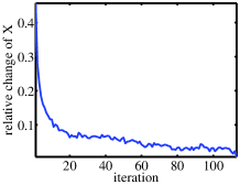
(a) Relative change of $X$

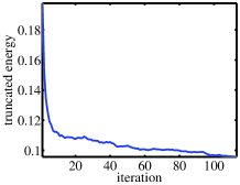
(b) Truncated energy

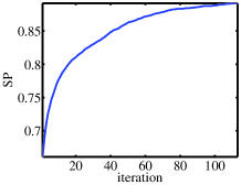
(c) SP

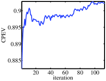
(d) CPEV

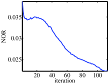
(e) NOR

Figure 1: Convergence of SPCArt(T-$\ell_{0}$) on image data. The convergence is relatively stable, and the criteria improve along with the iteration.

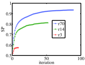
(a) SP

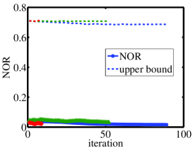
(b) NOR

(c) CPEV, $r=3$

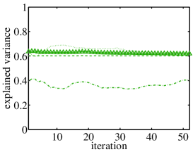
(d) CPEV, $r=14$

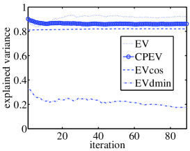
(e) CPEV, $r=70$

Figure 2: Performance bounds of SPCArt(T-en) for 3 levels of $r$ on image data. The legends of (c) and (d) are similar to that of (e). EV is a normalized version EV = $tr(X^{T}A^{T}AX)/tr(A^{T}A)$ so that it can be compared with CPEV. EVdmin = $d_{min}^{2}EV(V)/tr(A^{T}A)$ and EVcos = $\cos^{2}(\theta)EV(V)/tr(A^{T}A)$. We see EVcos is better than EVdmin in estimation, and EVcos meets empirical performance well. For NOR, the algorithm performs far optimistic than those upper bounds. Owning to the good orthogonality, EV are comparable to CPEV. For each $r$, as iteration goes, SP improves a lot while CPEV sacrifices little.

6.1 Synthetic Data

We will test whether SPCArt and rSVD-GP can recover some underlying sparse loadings. The synthetic data was introduced by [9] and became classical for sparse PCA problem. It considers three hidden Gaussian factors: $h_{1}\sim N(0,290)$, $h_{2}\sim N(0,300)$, $h_{3}=-0.3h_{1}+0.925h_{2}+\epsilon$, $\epsilon\sim N(0,1)$. Then ten variables are generated: $a_{i}=h_{j}+\epsilon_{i}$, $\epsilon_{i}\sim N(0,1)$, $i=1,\dots,10$, with $j=1$ for $i=1,\dots,4$, $j=2$ for $i=5,\dots,8$, $j=3$ for $i=9,10$. In words, $h_{1}$ and $h_{2}$ are independent, while $h_{3}$ has correlations with both of them, particularly $h_{2}$. The first 1-4 variables are generated by $h_{1}$, while the 5-8 variables are generated by $h_{2}$. So these two sets of variables are independent. The last variables 9-10 are generated by $h_{3}$, so they have correlations with both of the 1-4 and 5-8 variables, particularly the latter. The covariance matrix $C$ determined by $a_{i}$’s is fed into the algorithms. For those algorithms that only accept data matrix, an artificial data $\tilde{A}=V\Sigma^{-1/2}V^{T}$ is made where $V\Sigma V^{T}=C$ is the SVD of $C$. This is reasonable since they share the same loadings.

The algorithms are required to find two sparse loadings. Besides CPEV, the nonzero supports of the loadings are recorded, which should be consistent with the above generating model. The results are reported in Table 3. Except SPCA(T-$\ell_{1}$), the others, including SPCArt and rSVD-GP, successfully recovered the two most acceptable loading patterns 1-4,9-10; 5-10 and 1-4; 5-10, as can be seen from the CPEV.

6.2 Pitprops Data

The Pitprops data is a classical data to test sparse PCA [25]. There is a covariance matrix of 13 variables available: $C\in\mathbb{R}^{13\times 13}$. For those algorithms that only accept data matrix as input, an artificial data matrix $A=V\Sigma^{-1/2}V^{T}$ is made where $V\Sigma V^{T}=C$. The algorithms are tested to find $r=6$ sparse loadings. For fairness, $\lambda$’s are tuned so that each algorithm yields total cardinality of all loadings, denoted by NZ, about 18; and mainly T-sp and T-$\ell_{0}$ algorithms are tested. Criteria STD, NOR, and CPEV are reported. The results are shown in Table 4. For T-$\ell_{0}$, SPCArt does best overall, although its CPEV is not the best. The others, especially GPower(B), suffer from unbalanced cardinality, as can be seen from the loading patterns and STD; their CPEV may be high but they are mainly contributed by the dense leading vector, which aligns with the direction of maximal variance, i.e. leading PCA loading. The improvements of rSVD-GP(B) over GPower(B) on this point is significant, as can be seen from the tradeoff between STD and CPEV. For T-sp, focusing on NOR and CPEV, the performance of rSVD-GP is good while that of SPCArt is somewhat bad, for the CPEV is the worst although the NOR ranks two.

6.3 Natural Image Data

The investigation of the distribution of natural image patches is important for computer vision and pattern recognition communities. On this data set, we will evaluate the convergence of SPCArt, the performance bounds, and make a comprehensive comparisons between different algorithms. We randomly select 5000 gray-scale $13\times 13$ patches from BSDS [28]. Each patch is reshaped to a vector of dimension 169. The DC component of each patch is removed first, and then the mean of the data set is removed.

6.3.1 Convergence of SPCArt

We will show the stability of convergence and the improvement of SPCArt over simple thresholding [8]. We take T-$\ell_{0}$, $r=70$ as example. CPEV(V) = 0.95. The results are shown in Figure 1. Gradually, SPCArt has found a local optimal rotation such that less truncated energy from the rotated PCA loadings is needed (Figure 1(b)) to get a sparser (Figure 1(c)), more variance explained (Figure 1(d)), and more orthogonal (Figure 1(e)) basis. Note that, the results in the first iteration are equal to those of simple thresholding [8]. The final solution of SPCArt significantly improves over simple thresholding.

6.3.2 Performance Bounds of SPCArt

We now compare the theoretical bounds provided in Section 3.4 with empirical performance. T-en with $\lambda=0.15$ is taken as example, in which about 85% EV(V) is guaranteed. To achieve a more systematic evaluation, three levels of subspace dimension are tested: $r$ = [3 14 70] with the corresponding CPEV(V) = [0.42 0.71 0.95]. The results are shown in Figure 2. Note that most of the theoretical bounds are the absolute bounds without assuming the specific distribution of data, so they may be very different from the empirical performance.

First, for sparsity, the lower bound given in (15) is about 15%. But as seen in Figure 2(a), the empirical sparsity is far better than expectation, especially when $r$ is larger.

Similar situation occurs for nonorthogonality, as seen in Figure 2(b). The upper bounds are far too pessimistic to be practical. It may be caused by the high dimension of data.

Finally, for explained variance, it can be found from Figure 2(c), 2(d), 2(e) that there is no large discrepancy between EV and CPEV, owning to the near orthogonality of the sparse basis as indicated in Figure 2(b). On the other hand, the specific bound EVcos is better than the universal bound EVdmin. In contrast to sparsity and nonorthogonality, EVcos meets the empirical performance well, as analyzed in Section 3.4.

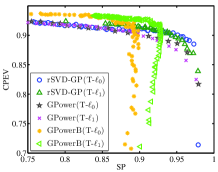
(a) CPEV

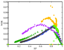
(b) NOR

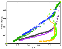
(c) Worst sparsity

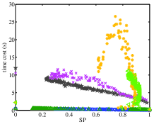
(d) Time cost

Figure 3: rSVD-GP v.s. GPower(B) on image data. From (c), we see that for GPower(B), the uniform parameter setting leads to unbalanced sparsity, the worst case is rather dense. rSVD-GP significantly improves over GPower(B) on the balance of sparsity as well as the other criteria.

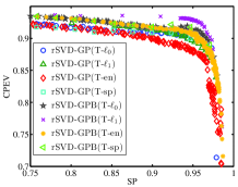
(a) CPEV

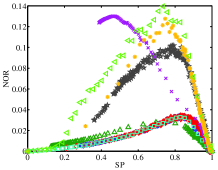
(b) NOR

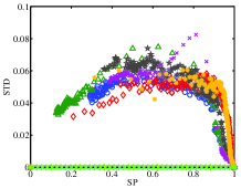
(c) STD

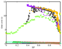
(d) Time cost

Figure 4: rSVD-GP v.s. rSVD-GPB on image data. Both are initialized with PCA. From (b), we see the block version gets much worse orthogonality than the deflation version. The other criteria are comparable except time cost.

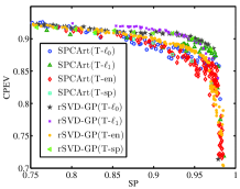
(a) CPEV

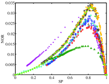
(b) NOR

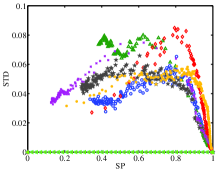
(c) STD

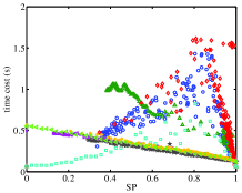
(d) Time cost

Figure 5: SPCArt v.s. rSVD-GP on image data. The two methods obtain comparable results on these criteria.

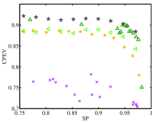
(a) CPEV

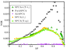
(b) NOR

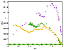
(c) STD

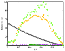
(d) Time cost

Figure 6: SPCArt v.s. SPCA, PathSPCA, ALSPCA on image data. To make the figures less messy, T-$\ell_{1}$ is taken as representative for SPCArt. SPCArt performs best overall, while PathSPCA performs best at CPEV. ALSPCA and SPCA are unstable. PathSPCA and SPCA are time consuming.

6.3.3 Performance Comparisons between Algorithms

We fix $r=70$ and run the algorithms over a range of parameter $\lambda$ to produce a series of results, then the algorithms are compared based on the same sparsity. We first verify the improvement of rSVD-GP over GPower(B) on the balance of sparsity, and take rSVD-GP(B) as example to show that the block group produces worse orthogonality than the deflation group. Then we compare SPCArt with the other algorithms.

(1) rSVD-GP v.s. GPower(B), see Figure 3. For GPower(B), the uniform parameter setting leads to unbalanced sparsity. In fact, the worst case is usually achieved by the leading loadings. rSVD-GP significantly improves over GPower(B) on this criterion as well as the others.

(2) rSVD-GP v.s. rSVD-GPB, see Figure 4. The block version always gets worse orthogonality. This is because there is no mechanism in it to ensure orthogonality.

(3) SPCArt v.s. rSVD-GP, see Figure 5. The two methods obtain comparable results on these criteria.

(4) SPCArt v.s. SPCA, PathSPCA, and ALSPCA, see Figure 6. SPCArt performs best overall. Generally, PathSPCA performs best at CPEV, but its time cost increases with cardinality. ALSPCA is unstable and sensitive to parameter, so is SPCA. Besides, SPCA is time consuming.

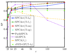
(a) SP

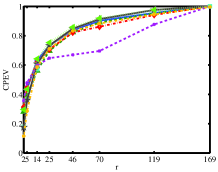
(b) CPEV

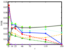
(c) NOR

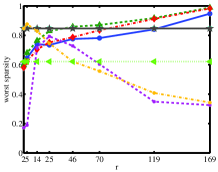
(d) Worst sparsity

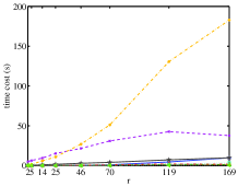
(e) Time cost

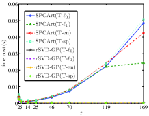
(f) Time cost per iteration

Figure 7: Evolution of solution as $r$ increases on image data, SPCArt v.s. PathSPCA, ALSPCA, SPCA, and rSVD-GP(T-$\ell_{0}$). In (f), only SPCArt and rSVD-GP are shown. SPCArt is insensitive to parameter setting. Compared with the deflation algorithms (PathSPCA, rSVD-GP), the loadings of SPCArt are adaptive with $r$, whose properties gradually improve. When $r$ becomes the full dimension, T-$\ell_{1}$ perfectly recovers the natural basis which is globally optimal, as can be seen from SP, worst sparsity, and NOR. Both the two sparsity criteria reach $(p-1)/p=0.994$ and NOR touches bottom 0. T-en achieves similar results.

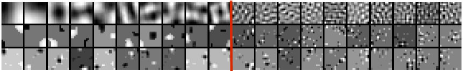
Figure 8: Images of the first 10 and the last 10 loadings among the total 70 loadings on image data. 1st line: PCA; 2nd line: rSVD-GP(T-sp); 3rd line: SPCArt(T-sp). $\lambda=\lfloor 0.85p\rfloor$. rSVD-GP is greedy, and the results of it are more confined to those of PCA, while SPCArt is more flexible.

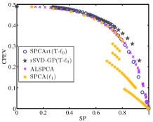
(a) CPEV

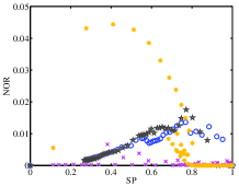
(b) NOR

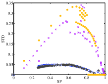
(c) STD

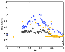
(d) Time cost

Figure 9: SPCArt(T-$\ell_{0}$) vs. rSVD-GP(T-$\ell_{0}$), ALSPCA, and SPCA on gene data, $r=6$. To be less messy, the other truncation types are not shown. ALSPCA is much more costly so it is not shown in (d). SPCArt(T-$\ell_{0}$) and rSVD-GP(T-$\ell_{0}$) perform best, and both finish within 1 second in such high dimensional data.

6.3.4 Evolution of Solution as $r$ Increases

Finally, we evaluate how the solution evolves as $r$ increases. $r$ is sampled so that CPEV(V) = [0.3 0.5 0.7 0.8 0.9 0.95 0.99 1]. For simplicity, the $\lambda$’s are kept fixed, they are set as follows. T-$\ell_{0}$: $1/\sqrt{p}$; T-sp: $\lfloor 0.85p\rfloor$; T-en: $0.15$; T-$\ell_{1}$: SPCArt $1/\sqrt{p}$, SPCA $4$, ALSPCA $0.7$. The results are plotted in Figure 7. We can observe that:

(1) Using the same threshold, T-$\ell_{1}$ is always more sparse and orthogonal than T-$\ell_{0}$, while explaining less variance.

(2) SPCArt is insensitive to parameter. A constant setting produces satisfactory results across $r$’s. But it is not the case for rSVD-GP.

(3) In contrast to the deflation algorithms (PathSPCA, rSVD-GP), SPCArt is a block algorithm. Its solution evolves as $r$. The sparsity, explained variance, orthogonality, and balance of sparsity improve as $r$ increases, and it has the potential to get optimal solution. This is evident for T-en and T-$\ell_{1}$ when $r$ becomes the full dimension 169. T-$\ell_{1}$ perfectly recovers the natural basis which is globally optimal; and T-en obtains similar results. Visualized images of the loadings of the deflation and block algorithm are shown in Figure 8. Due to the greedy nature, the results obtained by deflation algorithm are more confined to those of PCA; and the first 10 loadings differ significantly from the last 10 loadings.

6.4 Gene Data ($n\ll p$)

We now try the algorithms on the Leukemia dataset [26], which contains 7129 genes and 72 samples, i.e. $p\gg n$ data. This is a classical application that motivates the development of sparse PCA. Because from the thousands of genes, a sparse basis can help us to locate a few of them that determines the distribution of data. The results are shown in Figure 9. For this type of data, SPCA is run on the $p\gg n$ mode [9] for efficiency. PathSPCA is very slow except when SP$\geq 97\%$, so it is not involved in the comparison. SPCArt(T-$\ell_{0}$) and rSVD-GP(T-$\ell_{0}$) perform best (the later is slightly better).

6.5 Random Data ($n>p$)

Finally, we test the computational efficiency on a set of random data with increasing dimensions $p$ = [100 400 700 1000 1300]. Following [15, 10, 6], zero-mean, unit-variance Gaussian data is used for the test. To make how the computational cost depends on $p$ clear, we let $n=p+1$. For fair comparison, only T-sp with $\lambda=\lfloor 0.85p\rfloor$ are tested. $r$ is set to 20. The results are shown in Figure 10. rSVD-GP and PathSPCA increase nonlinearly against $p$, while SPCArt grows much slowly. Remember in Figure 6(d), we already showed that the time complexity of PathSPCA increases nonlinearly against the cardinality, and from Figure 7(f), we saw SPCArt increases nonlinearly against $r$. All these are consistent with Table 1. When dealing with high dimensional data and pursuing a few loadings, SPCArt is advantageous.

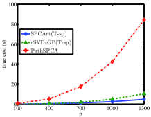
(a) Time cost

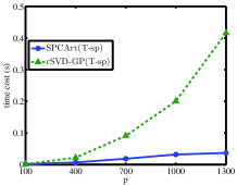
(b) Time cost per iteration

Figure 10: Speed test on random data with increasing dimension $p$. SPCArt grows much slowly as $p$.

7 Conclusion

According to the experiments, SPCArt significantly improves simple thresholding. rSVD-GP(B) improves GPower(B). rSVD-GP obtains loadings more orthogonal than rSVD-GPB. SPCArt, rSVD-GP, and PathSPCA generally perform well. PathSPCA consistently explains most variance, but it is the most time-consuming among the three. rSVD-GP and SPCArt perform similarly on sparsity, explained variance, orthogonality, and balance of sparsity. However rSVD-GP is more sensitive to parameter setting (except rSVD-GP(T-sp), i.e. TPower), and it is a greedy deflation algorithm. SPCArt belongs to the block group, its solution improves with the target dimension, and it has the potential to obtain globally optimal solution.

When the sample size is larger than the dimension, the time cost of PathSPCA and rSVD-GP go nonlinearly with the dimension, while SPCArt increases much slowly. They can deal with high dimensional data under different situations, SPCArt: the number of loadings is small; rSVD-GP: the sample size is small; PathSPCA: the target cardinality is small.

The four truncation types of SPCArt work well in different aspects: T-$\ell_{0}$ hard thresholding performs well overall; T-$\ell_{1}$ soft thresholding gets best sparsity and orthogonality; T-sp hard sparsity constraint directly controls sparsity and has zero sparsity variance; T-en truncation by energy guarantees explained variance, and the performance bound is tight.

There are two open questions unresolved. (1) Under what conditions can SPCArt, with each truncation type, recover the underlying sparse basis? Efforts have been made recently on this problem [29, 30, 11, 21]. (2) Is there any explicit objective formulation for T-en?

Appendix A Proof of the solution of T-sp

When $R$ is fixed, define $Z=VR^{T}$, (9) becomes $r$ independent subproblems:

$$\min_{X_{i}}\;\|Z_{i}-X_{i}\|^{2}_{F},\;s.t.\,\|X_{i}\|_{0}\leq p-\lambda,\;\|X_{i}\|_{2}=1.$$ (27)

Proposition 14.

$X_{i}^{*}=P_{\lambda}(Z_{i})/\|P_{\lambda}(Z_{i})\|_{2}$ is the solution of (27).

Proof.

The problem is equivalent to $\max_{X_{i}}Z_{i}^{T}X_{i}$, s.t. $\|X_{i}\|_{0}\leq p-\lambda,\|X_{i}\|_{2}=1$. We first prove that the non-zeros of $X_{i}^{*}$ are the normalized entries of $Z_{i}$ in the same support as $X_{i}^{*}$, then prove $\|X_{i}^{*}\|_{0}=p-\lambda$ and the support corresponds to the largest entries of $Z_{i}$. Assume the support of $X_{i}^{*}$ is $\mathcal{S}$. Divide $Z_{i}$ into two parts $Z_{i}=\tilde{Z}_{i}+\bar{Z}_{i}$, where $\tilde{Z}_{i}$ has the same support as $X_{i}^{*}$, and $\bar{Z}_{i}$ has the remaining support. The problem is reduced to $\max_{X_{i}}\tilde{Z}_{i}^{T}X_{i}$, s.t. $\text{support}(X_{i})=\mathcal{S}$, $\|X_{i}\|_{2}=1$. The solution is $X_{i}^{*}=\tilde{Z}_{i}/\|\tilde{Z}_{i}\|_{2}$. Next, since $Z_{i}^{T}\tilde{Z}_{i}/\|\tilde{Z}_{i}\|_{2}=\|\tilde{Z}_{i}\|_{2}$, to achieve a minima, $\|\tilde{Z}_{i}\|_{2}$ should be as large as possible. That is the largest $p-\lambda$ entries of $Z_{i}$. ∎

Appendix B Proofs of Performance Bounds of SPCArt

Many of the results can be proven by studying the special case $z=(1,0,\dots,0)^{T}$ and $z=(1/\sqrt{p},\dots,1/\sqrt{p})^{T}$. We mainly focus on the less straightforward ones.

B.1 Sparsity and Deviation

Proposition 7.

For T-$\ell_{0}$, the sparsity bounds are

$$\begin{cases}0\leq s(x)\leq 1-\frac{1}{p}&\text{, $\lambda<\frac{1}{\sqrt{p}}$,}\\ 1-\frac{1}{p\lambda^{2}}<s(x)\leq 1&\text{, $\lambda\geq\frac{1}{\sqrt{p}}$.}\end{cases}$$

Deviation $\sin(\theta(x,z))=\|\bar{z}\|_{2}$, where $\bar{z}$ is the truncated part: $\bar{z}_{i}=z_{i}$ if $x_{i}=0$, and $\bar{z}_{i}=0$ otherwise. The absolute bounds are:

$$0\leq\sin(\theta(x,z))\leq\begin{cases}\sqrt{p-1}\lambda&\text{, $\lambda<\frac{1}{\sqrt{p}}$,}\\ 1&\text{, $\lambda\geq\frac{1}{\sqrt{p}}$.}\end{cases}$$

All the above bounds are achievable.

Proof.

We only prove $1-\frac{1}{p\lambda^{2}}\leq s(x)$, if $\lambda\geq\frac{1}{\sqrt{p}}$. The others are easy to obtain. Let $\tilde{z}=z-\bar{z}$, i.e. the part above $\lambda$, and let $k=\|\tilde{z}\|_{0}$, then $k\lambda^{2}<\|\tilde{z}\|^{2}_{2}\leq 1$. So $k<1/\lambda^{2}$. Since $\|x\|_{0}=\|\tilde{z}\|_{0}$, $s(x)=1-\|x\|_{0}/p>1-1/(p\lambda^{2})$.∎

Proposition 8.

For T-$\ell_{1}$, the bounds of $s(x)$ and lower bound of $\sin(\theta(x,z))$ are the same as T-$\ell_{0}$. In addition, there are relative deviation bounds

$$\|\bar{z}\|_{2}\leq\sin(\theta(x,z))<\sqrt{\|\bar{z}\|^{2}_{2}+\lambda^{2}\|x\|_{0}}.$$

Proof.

Let $\tilde{z}=z-\bar{z}$, $\hat{z}=S_{\lambda}(z)$ and $y=\tilde{z}-\hat{z}$. Note that the absolute value of nonzero entry of $y$ is $\lambda$, and $\|y\|_{2}=\lambda\sqrt{\|\tilde{z}\|_{0}}=\lambda\sqrt{\|x\|_{0}}$. Then,

$$\cos(\theta(x,z))=\cos(\theta(\hat{z},z))=\hat{z}^{T}z/\|\hat{z}\|_{2}.$$ (28)

Expand $z=\hat{z}+y+\bar{z}$ and note that $\bar{z}$ is orthogonal to $\tilde{z}$ and $\hat{z}$, since their support do not overlap. We have,

$$\hat{z}^{T}z=\|\hat{z}\|^{2}_{2}+\hat{z}^{T}y.$$ (29)

By the soft thresholding operation,

$$0<\hat{z}^{T}y\leq\|\hat{z}\|_{2}\|y\|_{2}.$$ (30)

Combining (28), (29) and (30), we have $\|\hat{z}\|_{2}<\cos(\theta(x,z))\leq\|\hat{z}\|_{2}+\|y\|_{2}$. Note that the upper bound of (30) is achieved when $\hat{z}$ and $y$ are in the same direction, and in this case, $\|\hat{z}\|_{2}+\|y\|_{2}=\|\tilde{z}\|_{2}$. So $\|\hat{z}\|_{2}<\cos(\theta(x,z))\leq\|\tilde{z}\|_{2}$. Then $1-\|\tilde{z}\|^{2}_{2}\leq\sin^{2}(\theta(x,z))<1-\|\hat{z}\|^{2}_{2}$. The upper bound is approached when $\hat{z}$ becomes orthogonal to $y$, in this case $\|\hat{z}\|^{2}_{2}+\|y\|^{2}_{2}+\|\bar{z}\|^{2}_{2}=\|z\|^{2}_{2}=1$. Hence, $1-\|\hat{z}\|^{2}_{2}=\|\bar{z}\|^{2}_{2}+\|y\|^{2}_{2}=\|\bar{z}\|^{2}_{2}+\lambda^{2}\|x\|_{0}$. Besides, $1-\|\tilde{z}\|^{2}_{2}=\|\bar{z}\|^{2}_{2}$. The final result is $\|\bar{z}\|_{2}\leq\sin(\theta(x,z))<\sqrt{\|\bar{z}\|^{2}_{2}+\lambda^{2}\|x\|_{0}}$.∎

Proposition 10 can be proved in a way similar to T-en.

Proposition 11.

For T-en, $0\leq\sin(\theta(x,z))\leq\sqrt{\lambda}$. In addition

$$\lfloor{\lambda p}\rfloor/p\leq s(x)\leq 1-1/p.$$

If $\lambda<1/p$, there is no sparsity guarantee. When $p$ is moderately large, $\lfloor{\lambda p}\rfloor/p\approx\lambda$.

Proof.

Sort squared elements of $z$ in ascending order, and assume they are $\hat{z}^{2}_{1}\leq\hat{z}^{2}_{2}\leq\cdots\leq\hat{z}^{2}_{p}$ and the first $k$ of them are truncated. If $z$ is uniform, i.e. $\hat{z}^{2}_{1}=\hat{z}^{2}_{p}=1/p$, then the number of truncated entries is $k_{0}=\lfloor{\lambda p}\rfloor$. Suppose $\exists z$ achieves $k<k_{0}$, then $\sum^{k_{0}}_{i=1}\hat{z}^{2}_{i}$ is greater than that of uniform case i.e. $\sum^{k_{0}}_{i=1}\hat{z}^{2}_{i}>k_{0}/p$. By the ordering, $\hat{z}^{2}_{k_{0}}$ is above the mean of the first $k_{0}$ entries, $\hat{z}^{2}_{k_{0}}\geq 1/k_{0}\sum^{k_{0}}_{i=1}\hat{z}^{2}_{i}>1/p$. But on the other hand, $\hat{z}^{2}_{k_{0}+1}$ is below the mean of the remaining part, $\hat{z}^{2}_{k_{0}+1}\leq 1/(p-k_{0})\sum^{p}_{i=k_{0}+1}\hat{z}^{2}_{i}<1/(p-k_{0})(1-k_{0}/p)=1/p<\hat{z}^{2}_{k_{0}}$, i.e. $\hat{z}^{2}_{k_{0}+1}<\hat{z}^{2}_{k_{0}}$ which is a contradiction. Thus, $\lfloor{\lambda p}\rfloor/p\leq s(x)$.∎

B.2 Explained Variance

Theorem 12.

Let rank $r$ SVD of $A\in\mathbb{R}^{n\times p}$ be $U\Sigma V^{T}$, $\Sigma\in\mathbb{R}^{r\times r}$. Given $X\in\mathbb{R}^{p\times r}$, assume SVD of $X^{T}V$ is $WDQ^{T}$, $D\in\mathbb{R}^{r\times r}$, $d_{min}=\min_{i}D_{ii}$. Then

$$d_{min}^{2}\cdot EV(V)\leq EV(X),$$

and $EV(V)=\sum_{i}\Sigma^{2}_{ii}$.

Proof.

Let SVD of $A^{T}A$ be $[V,\,V_{2}]\begin{bmatrix}\Lambda&\\ &\Lambda_{2}\end{bmatrix}\begin{bmatrix}V^{T}\\ V^{T}_{2}\end{bmatrix}$, where $\Lambda=\Sigma^{2}$ and subscript 2 associates with the remaining loadings. Then

$$tr(X^{T}A^{T}AX) =tr(X^{T}[V,\,V_{2}]\begin{bmatrix}\Lambda&\\ &\Lambda_{2}\end{bmatrix}\begin{bmatrix}V^{T}\\ V^{T}_{2}\end{bmatrix}X)$$

$$=tr(X^{T}V\Lambda V^{T}X)+tr(X^{T}V_{2}\Lambda_{2}V^{T}_{2}X)$$

$$\geq tr(X^{T}V\Lambda V^{T}X)$$

$$=tr(WDQ^{T}\Lambda QDW^{T})$$

$$=tr(Q^{T}\Lambda QD^{2})$$

$$\geq tr(Q^{T}\Lambda Q)d^{2}_{min}$$

$$=d^{2}_{min}\sum_{i}\Lambda_{ii}.$$

∎

Theorem 13.

Let $C=Z^{T}X$, i.e. $C_{ij}=\cos(\theta(Z_{i},X_{j}))$, and let $\bar{C}$ be $C$ with diagonal elements removed. Assume $\theta(Z_{i},X_{i})=\theta$ and $\sum^{r}_{j}C_{ij}^{2}\leq 1$, $\forall i$, then

$$(\cos^{2}(\theta)-\sqrt{r-1}\sin(2\theta))\cdot EV(V)\leq EV(X).$$

When $\theta$ is sufficiently small,

$$(\cos^{2}(\theta)-O(\theta))\cdot EV(V)\leq EV(X).$$

Proof.

Following the notations of the previous theorem,

$$\quad\;\,tr(X^{T}A^{T}AX)$$

$$\geq tr(X^{T}V\Lambda V^{T}X)$$

$$=tr(X^{T}VR^{T}R\Lambda R^{T}RV^{T}X)$$

$$=tr(C^{T}R\Lambda R^{T}C)$$

$$=tr(R\Lambda R^{T}CC^{T})$$

$$=tr(R\Lambda R^{T}(I\cos(\theta)+\bar{C})(I\cos(\theta)+\bar{C}^{T}))$$

$$=tr(R\Lambda R^{T}(I\cos^{2}(\theta)+(\bar{C}+\bar{C}^{T})\cos(\theta)+\bar{C}\bar{C}^{T}))$$

$$\geq tr(\Lambda)\cos^{2}(\theta)+tr(R\Lambda R^{T}(\bar{C}+\bar{C}^{T}))\cos(\theta).$$

We estimate the minimum eigenvalue $\lambda_{min}$ of the symmetric matrix $S=\bar{C}+\bar{C}^{T}$. By Gershgorin circle theorem, $|\lambda_{min}|\leq\sum^{r}_{j\neq i}|S_{ij}|$, $\forall i$, since $S_{ii}=0$.

$$\sum^{r}_{j\neq i}|S_{ij}| =\sum^{r}_{j\neq i}|\cos(\theta(Z_{i},X_{j}))+\cos(\theta(X_{i},Z_{j}))|$$

$$\leq\sum^{r}_{j\neq i}|\cos(\theta(Z_{i},X_{j}))|+\sum^{r}_{j\neq i}|\cos(\theta(X_{i},Z_{j}))|$$

$$\leq\sqrt{r-1}\bigl{(}\sum^{r}_{j\neq i}|\cos(\theta(Z_{i},X_{j}))|^{2}\bigr{)}^{-1/2}$$

$$\quad+\sqrt{r-1}\bigl{(}\sum^{r}_{j\neq i}|\cos(\theta(X_{i},Z_{j}))|^{2}\bigr{)}^{-1/2}.$$

The last inequality holds since, $\forall x\in\mathbb{R}^{p}$, $\|x\|_{1}\leq\sqrt{p}\|x\|_{2}$. Because $Z$ is the $r$ orthonormal vectors, $\|Z^{T}X_{i}\|_{2}\leq\|X_{i}\|_{2}=1$, and $Z^{T}_{j}X_{i}=\cos(\theta(X_{i},Z_{j}))$, hence $\sum^{r}_{j\neq i}|\cos(\theta(X_{i},Z_{j}))|^{2}\leq 1-\cos^{2}(\theta)=\sin^{2}(\theta)$. And by assumption, $\sum^{r}_{j}C_{ij}^{2}\leq 1$, so we also have $\sum^{r}_{j\neq i}|\cos(\theta(Z_{i},X_{j}))|^{2}\leq\sin^{2}(\theta)$. Thus, $\sum^{r}_{j\neq i}|S_{ij}|\leq 2\sqrt{r-1}\sin(\theta)$, and $\lambda_{min}\geq-2\sqrt{r-1}\sin(\theta)$. Finally,

$$tr(X^{T}A^{T}AX) \geq tr(\Lambda)\cos^{2}(\theta)+tr(R\Lambda R^{T}(\bar{C}+\bar{C}^{T}))\cos(\theta)$$

$$\geq EV(V)\cos^{2}(\theta)+EV(V)\lambda_{min}\cos(\theta)$$

$$=\bigl{(}\cos^{2}(\theta)-2\sqrt{r-1}\cos(\theta)\sin(\theta)\bigr{)}EV(V)$$

$$=\bigl{(}\cos^{2}(\theta)-\sqrt{r-1}\sin(2\theta)\bigr{)}EV(V).$$

When $\theta$ is sufficiently small, such that $\sin(2\theta)\approx 2\theta$, we have $tr(X^{T}A^{T}AX)\geq(\cos^{2}(\theta)-O(\theta))EV(V)$.∎

Appendix C Deducing Original GPower from Matrix Approximation Formulation

First, we give the original GPower. Fixing $Y$, (22) and (23) have solutions $W_{i}^{*}=H_{\sqrt{\lambda_{i}}}(A^{T}Y_{i})/\|H_{\sqrt{\lambda_{i}}}(A^{T}Y_{i})\|_{2}$ and $W_{i}^{*}=S_{\lambda_{i}}(A^{T}Y_{i})/\|S_{\lambda_{i}}(A^{T}Y_{i})\|_{2}$ respectively. Substituting them into original objectives, the $\ell_{0}$ problem becomes

$$\max_{Y}\sum_{i}\sum_{j}\;[(A_{j}^{T}Y_{i})^{2}-\lambda_{i}]_{+},\;s.t.\,Y^{T}Y=I,$$ (31)

and the $\ell_{1}$ problem becomes $\max_{Y}\sum_{i}\sum_{j}\;[|A_{j}^{T}Y_{i}|-\lambda_{i}]_{+},\;s.t.\,Y^{T}Y=I$. Actually, it is to solve

$$\max_{Y}\sum_{i}\sum_{j}\;[|A_{j}^{T}Y_{i}|-\lambda_{i}]^{2}_{+},\;s.t.\,Y^{T}Y=I.$$ (32)

Now the problem is to maximize two convex functions, [6] approximately solves them via a gradient method which is generalized power method. The $t$th iteration is provided by

$$Y^{(t)}=Polar(AH_{\sqrt{\lambda_{i}}}(A^{T}Y^{(t-1)})),$$ (33)

and

$$Y^{(t)}=Polar(AS_{\lambda_{i}}(A^{T}Y^{(t-1)})).$$ (34)

We now see how these can be deduced from the matrix approximation formulations (24) and (25). Split $X$ into $X=WD$, $s.t.\|W_{i}\|_{2}=1$, $\forall i$ and $D>0$ is diagonal matrix whose diagonal element $d_{i}$ in fact models the length of the corresponding column of $X$. Then they become

$$\begin{split}\min_{Y,D,W}\;&\|A-YDW^{T}\|^{2}_{F}+\sum_{i}\lambda_{i}\|W_{i}\|_{0},\\ =&\|A\|_{F}^{2}+\sum_{i}d^{2}_{i}-2\sum_{i}d_{i}Y_{i}^{T}AW_{i}+\sum_{i}\lambda_{i}\|W_{i}\|_{0},\\ &s.t.\,Y^{T}Y=I,\;D>0\text{ is diagonal},\;\|W_{i}\|_{2}=1,\;\forall i,\end{split}$$ (35)

and

$$\begin{split}\min_{Y,D,W}\;&\frac{1}{2}\|A-YDW^{T}\|^{2}_{F}+\sum_{i}\lambda_{i}\|d_{i}W_{i}\|_{1},\\ =&\frac{1}{2}\|A\|_{F}^{2}+\frac{1}{2}\sum_{i}d^{2}_{i}-\sum_{i}d_{i}Y_{i}^{T}AW_{i}+\sum_{i}\lambda_{i}d_{i}\|W_{i}\|_{1},\\ &s.t.\,Y^{T}Y=I,\;D>0\text{ is diagonal},\;\|W_{i}\|_{2}=1,\;\forall i.\end{split}$$ (36)

Fix $Y$ and $W$, and solve $D$. For the $\ell_{0}$ case, $d_{i}^{*}=Y_{i}^{T}AW_{i}$. Substituting it back, we get (22).

For the $\ell_{1}$ case, $d_{i}^{*}=Y_{i}^{T}AW_{i}-\lambda_{i}\|W_{i}\|_{1}$. Assume $\lambda_{i}$ is sufficiently small, then $d_{i}>0$ is satisfied. Substituting it back we get $\max_{Y,W}\sum_{i}\big{(}Y_{i}^{T}AW_{i}-\lambda_{i}\|W_{i}\|_{1}\big{)}^{2},\;s.t.\,Y^{T}Y=I,\,\forall i,\,\|W_{i}\|_{2}=1$. When we fix $Y$ and solve $W$, under the previous assumption it is equivalent to (23). Substituting $W_{i}^{*}=S_{\lambda_{i}}(A^{T}Y_{i})/\|S_{\lambda_{i}}(A^{T}Y_{i})\|_{2}$ back, we obtain (32).

Finally, we can see that the solutions (33) and (34) literally combine the two solution steps of (24) and (25) respectively.

References

- [1] I. Jolliffe, Principal component analysis. Springer, 2002.
- [2] A. d’Aspremont, F. Bach, and L. Ghaoui, “Optimal solutions for sparse principal component analysis,” Journal of Machine Learning Research, vol. 9, pp. 1269–1294, 2008.
- [3] I. Jolliffe, N. Trendafilov, and M. Uddin, “A modified principal component technique based on the lasso,” Journal of Computational and Graphical Statistics, vol. 12, no. 3, pp. 531–547, 2003.
- [4] L. Mackey, “Deflation methods for sparse pca,” Advances in Neural Information Processing Systems, vol. 21, pp. 1017–1024, 2009.
- [5] I. T. Jolliffe, “Rotation of ill-defined principal components,” Applied Statistics, pp. 139–147, 1989.
- [6] M. Journée, Y. Nesterov, P. Richtárik, and R. Sepulchre, “Generalized power method for sparse principal component analysis,” Journal of Machine Learning Research, vol. 11, pp. 517–553, 2010.
- [7] H. Shen and J. Huang, “Sparse principal component analysis via regularized low rank matrix approximation,” Journal of multivariate analysis, vol. 99, no. 6, pp. 1015–1034, 2008.
- [8] J. Cadima and I. Jolliffe, “Loading and correlations in the interpretation of principle compenents,” Journal of Applied Statistics, vol. 22, no. 2, pp. 203–214, 1995.
- [9] H. Zou, T. Hastie, and R. Tibshirani, “Sparse principal component analysis,” Journal of computational and graphical statistics, vol. 15, no. 2, pp. 265–286, 2006.
- [10] Z. Lu and Y. Zhang, “An augmented lagrangian approach for sparse principal component analysis,” Mathematical Programming, pp. 1–45, 2009.
- [11] X. Yuan and T. Zhang, “Truncated power method for sparse eigenvalue problems,” Journal of Machine Learning Research, vol. 14, pp. 899–925, 2013.
- [12] R. Tibshirani, “Regression shrinkage and selection via the lasso,” Journal of the Royal Statistical Society. Series B (Methodological), pp. 267–288, 1996.
- [13] H. Zou and T. Hastie, “Regularization and variable selection via the elastic net,” Journal of the Royal Statistical Society: Series B (Statistical Methodology), vol. 67, no. 2, pp. 301–320, 2005.
- [14] D. Witten, R. Tibshirani, and T. Hastie, “A penalized matrix decomposition, with applications to sparse principal components and canonical correlation analysis,” Biostatistics, vol. 10, no. 3, p. 515, 2009.
- [15] A. d’Aspremont, L. El Ghaoui, M. Jordan, and G. Lanckriet, “A direct formulation for sparse pca using semidefinite programming,” SIAM Review, vol. 49, no. 3, pp. 434–448, 2007.
- [16] Y. Zhang and L. El Ghaoui, “Large-scale sparse principal component analysis with application to text data,” 2011.
- [17] B. Moghaddam, Y. Weiss, and S. Avidan, “Spectral bounds for sparse pca: Exact and greedy algorithms,” Advances in Neural Information Processing Systems, vol. 18, p. 915, 2006.
- [18] ——, “Generalized spectral bounds for sparse lda,” in Proceedings of the 23rd international conference on Machine learning. ACM, 2006, pp. 641–648.
- [19] Y. Zhang, A. d Aspremont, and L. Ghaoui, “Sparse pca: Convex relaxations, algorithms and applications,” Handbook on Semidefinite, Conic and Polynomial Optimization, pp. 915–940, 2012.
- [20] G. Golub and C. Van Loan, Matrix computations. Johns Hopkins Univ Pr, 1996, vol. 3.
- [21] Z. Ma, “Sparse principal component analysis and iterative thresholding,” The Annals of Statistics, vol. 41, no. 2, pp. 772–801, 2013.
- [22] C. Eckart and G. Young, “The approximation of one matrix by another of lower rank,” Psychometrika, vol. 1, no. 3, pp. 211–218, 1936.
- [23] D. L. Donoho, “For most large underdetermined systems of linear equations the minimal 1-norm solution is also the sparsest solution,” Communications on pure and applied mathematics, vol. 59, no. 6, pp. 797–829, 2006.
- [24] K. Fan, “A generalization of tychonoff’s fixed point theorem,” Mathematische Annalen, vol. 142, no. 3, pp. 305–310, 1961.
- [25] J. Jeffers, “Two case studies in the application of principal component analysis,” Applied Statistics, pp. 225–236, 1967.
- [26] T. Golub, D. Slonim, P. Tamayo, C. Huard, M. Gaasenbeek, J. Mesirov, H. Coller, M. Loh, J. Downing, M. Caligiuri, et al., “Molecular classification of cancer: class discovery and class prediction by gene expression monitoring,” Science, vol. 286, no. 5439, p. 531, 1999.
- [27] K. Sjöstrand, “Matlab implementation of lasso, lars, the elastic net and spca,” Informatics and Mathematical Modelling, Technical University of Denmark (DTU), 2005.
- [28] D. Martin, C. Fowlkes, D. Tal, and J. Malik, “A database of human segmented natural images and its application to evaluating segmentation algorithms and measuring ecological statistics,” in International Conference on Computer Vision. IEEE, 2001, pp. 416–423.
- [29] A. Amini and M. Wainwright, “High-dimensional analysis of semidefinite relaxations for sparse principal components,” The Annals of Statistics, vol. 37, no. 5B, pp. 2877–2921, 2009.
- [30] D. Paul and I. M. Johnstone, “Augmented sparse principal component analysis for high dimensional data,” arXiv preprint arXiv:1202.1242, 2012.