Error analysis for an ALE evolving surface finite element method

Abstract.

We consider an arbitrary-Lagrangian-Eulerian evolving surface finite element method for the numerical approximation of advection and diffusion of a conserved scalar quantity on a moving surface. We describe the method, prove optimal order error bounds and present numerical simulations that agree with the theoretical results.

1. Introduction

For each $t\in[0,T],T>0,$ let ${{\Gamma}(t)}$ be a smooth connected hypersurface in ${\mathbb{R}}^{m+1},m=1,2,3$, oriented by the normal vector field ${\boldsymbol{\nu}}(\cdot,t)$, with ${\Gamma}^{0}:={\Gamma}(0)$. We assume that there exists a diffeomorphism $\boldsymbol{G}(\cdot,t):{\Gamma}^{0}\to{{\Gamma}(t)},$ satisfying $\boldsymbol{G}\in\operatorname{C}^{2}([0,T],\operatorname{C}^{2}({\Gamma}^{0}))$. We set $\boldsymbol{v}(\boldsymbol{G}(\cdot,t),t)=\partial_{t}\boldsymbol{G}(\cdot,t)$ with $\boldsymbol{G}(\cdot,0)=\boldsymbol{I}$ (the identity). Furthermore we assume that $\boldsymbol{v}(\cdot,t)\in\operatorname{C}^{2}({{\Gamma}(t)})$. The given velocity field $\boldsymbol{v}=\boldsymbol{v}_{\boldsymbol{\nu}}+\boldsymbol{v}_{\boldsymbol{\mathcal{T}}}$ may contain both normal $\boldsymbol{v}_{\boldsymbol{\nu}}$ and tangential $\boldsymbol{v}_{\boldsymbol{\mathcal{T}}}$ components, i.e., $\boldsymbol{v}_{\boldsymbol{\nu}}=\boldsymbol{v}\cdot{\boldsymbol{\nu}}{\boldsymbol{\nu}}$ and $\boldsymbol{v}_{\boldsymbol{\mathcal{T}}}\cdot{\boldsymbol{\nu}}=0$.

We focus on the following linear parabolic partial differential equation on ${{\Gamma}(t)}$;

(1.1) $$\partial^{\bullet}_{\boldsymbol{v}}u+u\nabla_{{{\Gamma}(t)}}\cdot\boldsymbol{v}-\Updelta_{{{\Gamma}(t)}}u=0\quad\mbox{ on }{{\Gamma}(t)},$$

where, $\nabla_{{\Gamma}(t)}=\nabla-\nabla\cdot{\boldsymbol{\nu}}{\boldsymbol{\nu}}$ denotes the surface gradient, $\Updelta_{{\Gamma}(t)}=\nabla_{{\Gamma}(t)}\cdot\nabla_{{\Gamma}(t)}$ the Laplace Beltrami operator and

$$\partial^{\bullet}_{\boldsymbol{v}}u=\partial_{t}u+\boldsymbol{v}\cdot\nabla u=\partial_{t}u+\boldsymbol{v}_{\boldsymbol{\nu}}\cdot\nabla u+\boldsymbol{v}_{\boldsymbol{\mathcal{T}}}\cdot\nabla_{{\Gamma}(t)}u$$

is the material derivative with respect to the velocity field $\boldsymbol{v}$. For simplicity we will assume that the boundary of ${{\Gamma}(t)}$ is empty and hence no boundary conditions are needed. The method is easily adapted to surfaces with boundary. In the case that the surface has a boundary, under suitable assumptions (c.f., Remark 3.3), our analysis is valid for homogeneous Neumann boundary conditions, i.e.,

(1.2) $$\nabla_{{\Gamma}(t)}u\cdot{\boldsymbol{\mu}}=0\quad\text{ on }\partial{{\Gamma}(t)},$$

where ${\boldsymbol{\mu}}$ is the conormal to the boundary of the surface. The upshot is that the total mass is conserved i.e., $\frac{{\operatorname{d}}}{{\operatorname{d}}t}\int_{{\Gamma}(t)}u=0$. Note that the case ${\boldsymbol{\nu}}(\boldsymbol{x},t)$ being constant in space and time corresponds to the $n$-dimensional hypersurface ${{\Gamma}(t)}$ being flat. In this case (1.1) is a standard bulk PDE.

We expect that our results apply also to the case of Dirichlet boundary conditions however in this setting one must also estimate the error due to boundary approximation which we neglect in this work.

The following variational formulation of (1.1) was derived in [1] and makes use of the transport formula (A.1) and the integration by parts formula on the evolving surface [1, (2.2)] ;

(1.3) $$\frac{{\operatorname{d}}}{{\operatorname{d}}t}\int_{{\Gamma}(t)}u\varphi+\int_{{\Gamma}(t)}\nabla_{{\Gamma}(t)}u\cdot\nabla_{{\Gamma}(t)}\varphi=\int_{{\Gamma}(t)}u\partial^{\bullet}_{\boldsymbol{v}}\varphi,$$

where $\varphi$ is a sufficiently smooth test function defined on the space-time surface

$$\mathcal{G}_{T}:=\bigcup_{t\in[0,T]}{{\Gamma}(t)}\times\{t\}.$$

In [1], a finite element approximation was proposed for (1.3) using piecewise linear finite elements on a triangulated surface interpolating (at the nodes) ${{\Gamma}(t)}$, the vertices of the triangulated surface were moved with the material velocity (of points on ${{\Gamma}(t)}$) $\boldsymbol{v}$. In this work we adopt a similar setup, in that we propose a finite element approximation using piecewise linear finite elements on a triangulated surface interpolating (at the nodes) ${{\Gamma}(t)}$, however we move the vertices of the triangulated surface with the velocity $\boldsymbol{v}_{a}=\boldsymbol{v}+\boldsymbol{a}_{\boldsymbol{\mathcal{T}}}$, where $\boldsymbol{a}_{\boldsymbol{\mathcal{T}}}$ is an arbitrary tangential velocity field ($\boldsymbol{a}_{\boldsymbol{\mathcal{T}}}\cdot{\boldsymbol{\nu}}=0$). Furthermore we assume that $\boldsymbol{v}_{a}$ satisfies the same smoothness assumptions as the material velocity $\boldsymbol{v}$, i.e., there exits a diffeomorphism $\tilde{\boldsymbol{G}}(\cdot,t):{\Gamma}^{0}\to{{\Gamma}(t)},$ satisfying $\tilde{\boldsymbol{G}}\in\operatorname{C}^{2}([0,T],\operatorname{C}^{2}({\Gamma}^{0}))$ with $\boldsymbol{v}_{a}(\tilde{\boldsymbol{G}}(\cdot,t),t)=\partial_{t}\tilde{\boldsymbol{G}}(\cdot,t)$ and with $\tilde{\boldsymbol{G}}(\cdot,0)=\boldsymbol{I}$ (the identity) and $\boldsymbol{v}_{a}(\cdot,t)\in\operatorname{C}^{2}({{\Gamma}(t)})$. We remark, that if ${{\Gamma}(t)}$ has a boundary this assumption implies that the arbitrary velocity $\boldsymbol{a}_{\boldsymbol{\mathcal{T}}}$ has zero conormal component on the boundary, i.e., for $t\in[0,T]$,

(1.4) $$(\boldsymbol{v}-\boldsymbol{v}_{a})\cdot{\boldsymbol{\mu}}=0\quad\text{ on }\partial{{\Gamma}(t)}.$$

For a sufficiently smooth function $f$, we have that

$$\partial^{\bullet}_{\boldsymbol{v}_{a}}f =\partial_{t}f+\boldsymbol{v}_{a}\cdot\nabla f=\partial_{t}f+\boldsymbol{v}_{\boldsymbol{\nu}}\cdot\nabla f+(\boldsymbol{a}_{\boldsymbol{\mathcal{T}}}+\boldsymbol{v}_{\boldsymbol{\mathcal{T}}})\cdot\nabla_{{\Gamma}(t)}f=\partial^{\bullet}_{\boldsymbol{v}}f+\boldsymbol{a}_{\boldsymbol{\mathcal{T}}}\cdot\nabla_{{\Gamma}(t)}f.$$

Thus we may write the following equivalent variational formulation to (1.1), which will form the basis for our finite element approximation

(1.5) $$\frac{{\operatorname{d}}}{{\operatorname{d}}t}\int_{{\Gamma}(t)}u\varphi+\int_{{\Gamma}(t)}\nabla_{{\Gamma}(t)}u\cdot\nabla_{{\Gamma}(t)}\varphi=\int_{{\Gamma}(t)}\left(u\partial^{\bullet}_{\boldsymbol{v}_{a}}\varphi-u\boldsymbol{a}_{\boldsymbol{\mathcal{T}}}\cdot\nabla_{{\Gamma}(t)}\varphi\right),$$

where $\varphi$ is a sufficiently smooth test function defined on $\mathcal{G}_{T}$. We note that (1.5) may be thought of as a weak formulation of an advection diffusion-equation on a surface with material velocity $\boldsymbol{v}_{a}$, in which the advection $\boldsymbol{a}_{\boldsymbol{\mathcal{T}}}$ is governed by some external process other than material transport. Hence the results we present are also an analysis of a numerical scheme for an advection diffusion equation on an evolving surface with another source of advective transport other than that due to the material velocity.

The original (Lagrangian) evolving surface finite element method (ESFEM) was proposed and analysed in [1], where optimal error bounds were shown for the error in the energy norm in the semidiscrete (space discrete) case. Optimal $\operatorname{L}_{2}$ error bounds for the semidiscrete case were shown in [2] and an optimal error bound for the full discretisation was shown in [3]. High order Runge-Kutta time discretisations and BDF timestepping schemes for the ESFEM were analysed in [4] and [5] respectively. There has also been recent work on the analysis of ESFEM approximations of the Cahn-Hilliard equation on an evolving surface [6], scalar conservation laws on evolving surfaces [7] and the wave equation on an evolving surface [8]. For an overview of finite element methods for PDEs on fixed and evolving surfaces see [9]. Although the analytical results have thus far focussed on the case where the discrete velocity is an interpolation of the continuous material velocity, the Lagrangian setting, in many applications it proves computationally efficient to consider a mesh velocity which is different to the interpolated material velocity. In particular it appears that the arbitrary tangential velocity, that we consider in this study can be chosen such that beneficial mesh properties are observed in practice. This provides the motivation for this work in which we analyse an ESFEM where the material velocity of the mesh is different to (the interpolant of) the material velocity of the surface, i.e., an arbitrary Lagrangian-Eulerian ESFEM (ALE-ESFEM). We refer to [10] for extensive computational investigations of the ALE-ESFEM that we analyse in this study. For examples in the numerical simulation of mathematical models for cell motility and biomembranes, where the ALE approach proves computationally more robust than the Lagrangian approach, we refer to [11, 12, 13, 14].

Our main results are Theorems 4.3 and 5.4 where we show optimal order error bounds for the semidiscrete (space discrete, time continuous) and fully discrete numerical schemes. The fully discrete bound is proved for a second order backward difference time discretisation. An optimal error bound is also stated for an implicit Euler time discretisation. While the fully discrete bound is proved independently of the bound on the semidiscretisation, we believe that the analysis of the semidiscrete scheme may prove a useful starting point for the analysis of other time discretisations. We also observe that, under suitable assumptions on the evolution, the analysis holds for smooth flat surfaces, i.e, bulk domains with smooth boundary. Thus the analysis we present is also an analysis of ALE schemes for PDEs in evolving bulk domains.

We report on numerical simulations of the fully discrete scheme that support our theoretical results and illustrate that the arbitrary tangential velocity may be chosen such that the meshes generated during the evolution are more suitable than in the Lagrangian case. Proposing a general recipe for choosing the tangential velocity is a challenging task that is beyond the scope of this article and we do not address this issue. Moreover the choice of the tangential velocity and what constitutes a good computational mesh is likely to depend heavily on the specific application. We also investigate numerically the long time behaviour of solutions to (1.1) with different initial data when the evolution of the surface is a periodic function of time. Our numerical results indicate that in the example we consider the solution converges to the same periodic solution for different initial data.

The original ESFEM was formulated for a surface with a smooth material velocity that had both normal and tangential components [1]. Hence many of the results from the literature are applicable in the present setting of a smooth arbitrary tangential velocity.

2. Setup

We start by introducing an abstract notation in which we formulate the problem.

2.1 Definition (Bilinear forms).

For $\varphi,\psi\in\operatorname{H}^{1}{({{\Gamma}(t)})},\boldsymbol{w}\in\operatorname{C}^{2}{({{\Gamma}(t)})}$ we define the following bilinear forms

$$a\left({\varphi(\cdot,t)},{\psi(\cdot,t)}\right) =\int_{{\Gamma}(t)}\nabla_{{\Gamma}(t)}\varphi(\cdot,t)\cdot\nabla_{{\Gamma}(t)}\psi(\cdot,t)$$

$$m\left({\varphi(\cdot,t)},{\psi(\cdot,t)}\right) =\int_{{\Gamma}(t)}\varphi(\cdot,t)\psi(\cdot,t)$$

$$g\left({\varphi(\cdot,t)},{\psi(\cdot,t)};{\boldsymbol{w}(\cdot,t)}\right) =\int_{{\Gamma}(t)}\varphi(\cdot,t)\psi(\cdot,t)\nabla_{{\Gamma}(t)}\cdot\boldsymbol{w}(\cdot,t)$$

$$b\left({\varphi(\cdot,t)},{\psi(\cdot,t)};{\boldsymbol{w}(\cdot,t)}\right) =\int_{{\Gamma}(t)}\varphi(\cdot,t)\nabla_{{\Gamma}(t)}\psi(\cdot,t)\cdot\boldsymbol{w}(\cdot,t)$$

$$\tilde{a}\left({\varphi(\cdot,t)},{\varphi(\cdot,t)};{\boldsymbol{v}^{a}(\cdot,t)}\right) =\int_{{\Gamma}(t)}\left(\nabla_{{\Gamma}(t)}\cdot\boldsymbol{v}^{a}(\cdot,t)-2\mathcal{D}_{{{\Gamma}(t)}}{\left(\boldsymbol{v}^{a}(\cdot,t)\right)}\right)\nabla_{{\Gamma}(t)}\varphi(\cdot,t)\cdot\nabla_{{\Gamma}(t)}\psi(\cdot,t)$$

$$\tilde{b}\left({\varphi(\cdot,t)},{\psi(\cdot,t)};{\boldsymbol{w}(\cdot,t)};{\boldsymbol{v}^{a}(\cdot,t)}\right) =\int_{{\Gamma}(t)}\nabla_{{\Gamma}(t)}\cdot\boldsymbol{v}^{a}(\cdot,t)\left(\varphi(\cdot,t)\boldsymbol{w}(\cdot,t)\cdot\nabla_{{\Gamma}(t)}\psi(\cdot,t)\right)$$

$$-\int_{{{\Gamma}_{h}(t)}}\varphi(\cdot,t)\boldsymbol{w}(\cdot,t)\cdot\mathcal{B}_{{{\Gamma}(t)}}{\left(\boldsymbol{v}^{a}(\cdot,t)\right)}\nabla_{{\Gamma}(t)}\psi(\cdot,t),$$

with the deformation tensors $\mathcal{B}_{(\cdot)}{\left(\cdot\right)}$ and $\mathcal{D}_{(\cdot)}{\left(\cdot\right)}$ as defined in Lemma A.1.

We may now write the equation (1.5) as

(2.1) $$\frac{{\operatorname{d}}}{{\operatorname{d}}t}m\left({u},{\varphi}\right)+a\left({u},{\varphi}\right)=m\left({u},{\partial^{\bullet}_{\boldsymbol{v}_{a}}\varphi}\right)-b\left({u},{\varphi};{\boldsymbol{a}_{\boldsymbol{\mathcal{T}}}}\right).$$

In [1] the authors showed existence of a weak solution to (1.3) and hence a weak solution exists to the (reformulated) problem (1.5), furthermore for sufficiently smooth initial data the authors proved the following estimate for the solution of (1.3) and hence of (1.5)

(2.2) $$\sup_{t\in(0,T)}\left\|u(\cdot,t)\right\|_{\operatorname{L}_{2}\left({{\Gamma}(t)}\right)}^{2}+\int_{0}^{T}\left\|\nabla_{{\Gamma}(t)}u\right\|_{\operatorname{L}_{2}\left({{\Gamma}(t)}\right)}^{2}{\operatorname{d}}t\leq c\left\|u_{0}\right\|_{\operatorname{L}_{2}\left({\Gamma}^{0}\right)}^{2},$$

(2.3) $$\int_{0}^{T}\left\|\partial^{\bullet}_{\boldsymbol{v}}u\right\|_{\operatorname{L}_{2}\left({{\Gamma}(t)}\right)}^{2}{\operatorname{d}}t+\sup_{t\in(0,T)}\left\|\nabla_{\Gamma}u\right\|_{\operatorname{L}_{2}\left({\Gamma}\right)}\leq c\left\|u_{0}\right\|_{\operatorname{H}^{1}({\Gamma}^{0})}^{2}.$$

We immediately conclude that as $\partial^{\bullet}_{\boldsymbol{v}_{a}}u-\partial^{\bullet}_{\boldsymbol{v}}u=\boldsymbol{a}_{\boldsymbol{\mathcal{T}}}\cdot\nabla_{\Gamma}u$ the bound (2.3) holds with the material derivative with respect to the material velocity replaced with the material derivative with respect to the ALE-velocity. See [15, 16, 17] for further discussion on the well-posedness of the weak formulation of the continuous problem.

3. Surface finite element discretisation

3.1. Surface discretisation

The smooth surface $\Gamma(t)$ is interpolated at nodes $\boldsymbol{X}_{j}(t)\in{{\Gamma}(t)}$ ($j=1,\ldots,J$) by a discrete evolving surface ${{\Gamma}_{h}(t)}$. These nodes move with velocity ${\operatorname{d}}\boldsymbol{X}_{j}(t)/{\operatorname{d}}t=\boldsymbol{v}_{a}(\boldsymbol{X}_{j}(t),t)$ and hence the nodes of the discrete surface ${{\Gamma}_{h}(t)}$ remain on the surface ${{\Gamma}(t)}$ for all $t\in[0,T]$. The discrete surface,

$$\Gamma_{h}(t)=\bigcup_{K(t)\in\mathcal{T}_{h}(t)}K(t)$$

is the union of $m$-dimensional simplices $K(t)$ that is assumed to form an admissible triangulation $\mathcal{T}_{h}(t)$; see [9, §4.1] for details. We assume that the maximum diameter of the simplices is bounded uniformly in time and we denote this bound by $h$ which we refer to as the mesh size.

We assume that for each point $x$ on ${{\Gamma}_{h}(t)}$ the exists a unique point $\boldsymbol{p}(\boldsymbol{x},t)$ on ${{\Gamma}(t)}$ such that for $t\in[0,T]$ (see [9, Lemma 2.8] for sufficient conditions such that this assumption holds)

(3.1) $$\boldsymbol{x}=\boldsymbol{p}(\boldsymbol{x},t)+d(\boldsymbol{x},t){\boldsymbol{\nu}}(\boldsymbol{p}(\boldsymbol{x},t),t),$$

where $d$ is the oriented distance function to ${{\Gamma}(t)}$ (see [9, §2.2] for details).

For a continuous function $\eta_{h}$ defined on ${{\Gamma}_{h}(t)}$ we define its lift $\eta_{h}^{l}$ onto ${{\Gamma}(t)}$ by extending constantly in the normal direction ${\boldsymbol{\nu}}$ (to the continuous surface) as follows

(3.2) $$\eta_{h}^{l}(\boldsymbol{p},t)=\eta_{h}(\boldsymbol{x}(\boldsymbol{p},t),t)\quad\text{for }\boldsymbol{p}\in{{\Gamma}(t)},$$

where $\boldsymbol{x}(\boldsymbol{p},t)$ is defined by (3.1).

We assume that the triangulated and continuous surfaces are such that for each simplex $K(t)\in\mathcal{T}_{h}(t)$ there is a unique $k(t)\subset{{\Gamma}(t)}$, whose edges are the unique projections of the edges of $K(t)$ onto ${{\Gamma}(t)}$. The union of the $k(t)$ induces an exact triangulation of ${{\Gamma}(t)}$ with curved edges. We refer, for example, to [9, §4.1] for further details.

We also find it convenient to introduce the discrete space-time surface

$$\mathcal{G}_{h,T}:=\bigcup_{t\in[0,T]}{{\Gamma}_{h}(t)}\times\{t\}.$$

3.2 Definition (Surface finite element spaces).

For each $t\in[0,T]$ we define the finite element spaces together with their associated lifted finite element spaces

$${\mathcal{S}_{h}(t)} =\left\{\Phi\in C^{0}\left({{\Gamma}_{h}(t)}\right)|\Phi|_{K}\mbox{ is linear affine for each }K\in{\mathcal{T}}_{h}(t)\right\},$$

$${\mathcal{S}_{h}^{l}(t)} =\left\{\varphi=\Phi^{l}|\Phi\in{\mathcal{S}_{h}(t)}\right\}.$$

Let $\chi_{j}(\cdot,t)$ ($j=1,\dots,N$) be the nodal basis of ${\mathcal{S}_{h}(t)}$, so that, denoting by $\{\boldsymbol{X}_{j}\}_{j=1}^{J}$ the vertices of ${{\Gamma}_{h}(t)}$, $\chi_{j}(\boldsymbol{X}_{i}(t),t)=\delta_{ji}$. The discrete surface moves with the piecewise linear velocity $\boldsymbol{V}^{a}_{h}$ and by $\boldsymbol{T}^{a}_{h}$ we denote the interpolant of the arbitrary tangential velocity $\boldsymbol{a}_{\boldsymbol{\mathcal{T}}}$

(3.3) $$\boldsymbol{V}^{a}_{h}(\boldsymbol{x},t) =\sum_{j=1}^{J}\boldsymbol{v}_{a}(\boldsymbol{X}_{j}(t),t)\chi_{j}(\boldsymbol{x},t),$$

(3.4) $$\boldsymbol{T}^{a}_{h}(\boldsymbol{x},t) =\sum_{j=1}^{J}\boldsymbol{a}_{\boldsymbol{\mathcal{T}}}(\boldsymbol{X}_{j}(t),t)\chi_{j}(\boldsymbol{x},t).$$

The discrete surface gradient is defined piecewise on each surface simplex $K(t)\in\mathcal{T}_{h}(t)$ as

$$\nabla_{\Gamma_{h}}g=\nabla g-\nabla g\cdot{\boldsymbol{\nu}}_{h}{\boldsymbol{\nu}}_{h},$$

where ${\boldsymbol{\nu}}_{h}$ denotes the normal to the discrete surface defined element wise.

We now relate the material velocity $\boldsymbol{V}^{a}_{h}$ of the triangulated surface ${{\Gamma}_{h}}$ to the material velocity $\boldsymbol{v}^{a}_{h}$ of the smooth triangulated surface. For each $\boldsymbol{X}(t)$ on ${{\Gamma}_{h}(t)}$ there is a unique $\boldsymbol{Y}(t)=\boldsymbol{p}(\boldsymbol{X}(t),t)\in{{\Gamma}(t)}$ with

(3.5) $$\frac{{\operatorname{d}}}{{\operatorname{d}}t}{\boldsymbol{Y}}(t)=\partial_{t}\boldsymbol{p}(\boldsymbol{X}(t),t)+\boldsymbol{V}^{a}_{h}(\boldsymbol{X}(t),t)\cdot\nabla\boldsymbol{p}(\boldsymbol{X}(t),t)=:\boldsymbol{v}^{a}_{h}(\boldsymbol{p}(\boldsymbol{X}(t),t),t),$$

where $\boldsymbol{p}$ is as in (3.1). We note that $\boldsymbol{v}^{a}_{h}$ is not the interpolant of the velocity $\boldsymbol{v}_{a}$ into the space ${\mathcal{S}_{h}^{l}}$ (c.f., [2, Remark 4.4]). We denote by $\boldsymbol{t}^{a}_{h}=(\boldsymbol{T}^{a}_{h})^{l}$ the lift of the velocity $\boldsymbol{T}^{a}_{h}$ to the smooth surface.

3.3 Remark (Surfaces with boundary).

While the method is directly applicable to surfaces with boundary, for the analysis we require the lift of the triangulated surface to be the smooth surface i.e., $({{\Gamma}_{h}(t)})^{l}={{\Gamma}(t)}$. Thus in general we must allow the faces of elements on the boundary of the triangulated surface to be curved. For the natural boundary conditions we consider it is possible to define a conforming piecewise linear finite element space on a triangulation with curved boundary elements, see for example [19], assuming this setup and neglecting the variational crime committed in integrating over curved faces the analysis we present in the subsequent sections remains valid. However as the surface is evolving a further requirement is that the continuous material velocity $\boldsymbol{v}$ and the material velocity of the smooth triangulated (lifted) surface $\boldsymbol{v}^{a}_{h}$ must satisfy

(3.6) $$(\boldsymbol{v}-\boldsymbol{v}_{h}^{a})\cdot{\boldsymbol{\mu}}=0\quad\text{ on }\partial{{\Gamma}(t)},$$

where ${\boldsymbol{\mu}}$ is the conormal to the surface. If (3.6) does not hold, the additional error due to domain approximation must also be estimated. We remark that this issue is not specific to the ALE scheme we consider in this study and also arises if we take $\boldsymbol{a}_{\boldsymbol{\mathcal{T}}}=\boldsymbol{0}$, i.e., the Lagrangian setting.

We note that although restrictive the above assumptions are satisfied for some nontrivial examples that are of interest in applications. In §6 we present two such examples. In Example 6.1, we present an example of a moving surface with boundary where the lift of the polyhedral surface (with straight boundary faces) is the smooth surface. In Example 6.4, we present an example where the surface is the graph of a time dependent function over the unit disc. Here the boundary curve is fixed and the boundary edges of elements on the boundary of the triangulated surface are curved such that the triangulation of the boundary is exact.

3.4 Remark (ALE schemes for PDEs posed in bulk domains).

As a special case of a surface with boundary, the method is applicable to a moving domain in $n$ $(n=1,2,3)$ dimensions, that is when ${{\Gamma}(t)}$ is a flat (i.e., the normal to the surface is constant) $n$ dimensional hypersurface in ${\mathbb{R}}^{n+1}$ with smooth boundary. We note that the formulae for the discrete schemes (4.1), (5.1) and (5.63) are the same as in the case of a curved hypersurface. Under suitable assumptions on the velocity at the boundary, the analysis we present is valid in this setting. Specifically the analysis we present is valid for a flat three dimensional surface with zero normal velocity but nonzero tangential (and conormal) velocity (subject to (3.6)). In this case, as the domain is flat the geometric errors we estimate in the subsequent sections are zero (as ${{\Gamma}_{h}(t)}=({{\Gamma}_{h}(t)})^{l}={{\Gamma}(t)}$ since the lift is in the normal direction only). We note that this assumption necessitates curved boundary elements in this case. Therefore, as a consequence of our analysis we get an error estimate for an ALE scheme for a linear parabolic equation on an evolving three dimensional bulk domain in which all of the analysis is all carried out on the physical domain.

3.5. Material derivatives

We introduce the normal time derivative $\partial^{\circ}$ on a surface moving with material velocity $\boldsymbol{v}$ defined by

$$\partial^{\circ}\eta:=\partial_{t}\eta+\boldsymbol{v}\cdot{\boldsymbol{\nu}}{\boldsymbol{\nu}}\cdot\nabla\eta,$$

and define the space

$$\operatorname{H}^{1}{(\mathcal{G}_{T})}:=\left\{\eta\in\operatorname{L}_{2}(\mathcal{G}_{T})\left|\nabla_{\Gamma}\eta\in\operatorname{L}_{2}(\mathcal{G}_{T})\right|\partial^{\circ}\eta\in\operatorname{L}_{2}(\mathcal{G}_{T})\right\}.$$

We are now in a position to define material derivatives on the triangulated surfaces. Given the velocity field $\boldsymbol{V}^{a}_{h}\in({\mathcal{S}_{h}})^{m+1}$ and the associated velocity $\boldsymbol{v}^{a}_{h}$ on ${{\Gamma}(t)}$ we define discrete material derivatives on ${{\Gamma}_{h}(t)}$ and ${{\Gamma}(t)}$ element wise as follows, for $\Phi_{h}(\cdot,t)\in{\mathcal{S}_{h}(t)}$ with $\partial^{\circ}\Phi_{h}|_{K(t)}\in\operatorname{L}_{2}(K(t))$ and $\varphi(\cdot,t)\in\operatorname{H}^{1}{(\mathcal{G}_{T})}$,

(3.7) $$\partial^{\bullet}_{h,\boldsymbol{V}^{a}_{h}}\Phi_{h}|_{K(t)} =\left(\partial_{t}\Phi_{h}+\boldsymbol{V}^{a}_{h}\cdot\nabla\Phi_{h}\right)|_{K(t)},$$

(3.8) $$\partial^{\bullet}_{h,\boldsymbol{v}^{a}_{h}}\varphi|_{k(t)} =\left(\partial_{t}\varphi+\boldsymbol{v}^{a}_{h}\cdot\nabla\varphi\right)|_{k(t)}.$$

We find it convenient to introduce the spaces

$${\mathcal{S}_{h}^{T}}:=\left\{\Phi_{h}\text{ and }\partial^{\bullet}_{\boldsymbol{V}^{a}_{h}}\Phi_{h}\in\operatorname{C}^{0}(\mathcal{G}_{h,T})|\Phi_{h}(\cdot,t)\in{\mathcal{S}_{h}(t)},t\in[0,T]\right\}$$

and

$${(\mathcal{S}_{h}^{T})^{l}}:=\left\{\varphi_{h}\text{ and }\partial^{\bullet}_{\boldsymbol{v}^{a}_{h}}\varphi_{h}\in\operatorname{C}^{0}(\mathcal{G}_{T})|\varphi_{h}(\cdot,t)\in{\mathcal{S}_{h}^{l}(t)},t\in[0,T]\right\}.$$

The following transport property of the finite element basis functions was shown in [1, §5.2]

(3.9) $$\partial^{\bullet}_{h,\boldsymbol{V}^{a}_{h}}\chi_{j}=0,\quad\partial^{\bullet}_{h,\boldsymbol{v}^{a}_{h}}\chi_{j}^{l}=0,$$

which implies that for $\Phi_{h}=\sum_{j}\Phi_{j}(t)\chi_{j}(\cdot,t)\in{\mathcal{S}_{h}(t)}$ with $\varphi_{h}=\Phi_{h}^{l}\in{\mathcal{S}_{h}^{l}(t)}$

(3.10) $$\partial^{\bullet}_{h,\boldsymbol{V}^{a}_{h}}\Phi_{h}(\cdot,t)=\sum_{j=1}^{J}\left(\frac{{\operatorname{d}}}{{\operatorname{d}}t}{\Phi}_{j}(t)\right)\chi_{j}(\cdot,t),\quad\partial^{\bullet}_{h,\boldsymbol{v}^{a}_{h}}\varphi_{h}(\cdot,t)=\sum_{j=1}^{J}\left(\frac{{\operatorname{d}}}{{\operatorname{d}}t}{\Phi}_{j}(t)\right)\chi_{j}(\cdot,t)^{l}.$$

We now introduce the notation we need to formulate and analyse the fully discrete scheme. Let $N$ be a positive integer, we define the uniform timestep $\tau=T/N$. For each $n\in\{0,\dots,N\}$ we set $t^{n}=n\tau$. We also occasionally use the same shorthand for time dependent objects, e.g., ${{\Gamma}^{n}}:={\Gamma}(t^{n})$ and ${{\Gamma}_{h}^{n}}:={{\Gamma}_{h}}(t^{n})$, $\left(\boldsymbol{T}_{a}^{h}\right)^{n}:=\boldsymbol{T}_{a}^{h}(\cdot,t^{n})$ etc. For a discrete time sequence $f^{n}$, $n\in\{0,\dots,N\}$ we introduce the notation

(3.11) $$\partial_{\tau}f^{n}=\frac{1}{\tau}\left(f^{n+1}-f^{n}\right).$$

For $n\in\{0,\dots,N\}$ we denote by ${\mathcal{S}^{n}_{h}}={\mathcal{S}_{h}}(t^{n})$ and by ${\mathcal{S}_{h}^{n,l}}={\mathcal{S}_{h}^{l}}(t^{n})$. For $j=\{1,\dots,J\}$, we set

(3.12) $$\chi_{j}^{n}=\chi_{j}(\cdot,t^{n}),\quad\chi_{j}^{n,l}=\chi^{l}_{j}(\cdot,t^{n})$$

and employ the notation

(3.13) $$\Phi_{h}^{n}=\sum_{j=1}^{J}\Phi_{j}^{n}\chi_{j}^{n}\in{\mathcal{S}^{n}_{h}},\quad\varphi_{h}^{n}=\Phi^{n,l}\in{\mathcal{S}_{h}^{n,l}}.$$

Following [3] we find it convenient to define for $\alpha=-1,0,1$ and $t\in[t^{n-1},t^{n+1}]$

(3.14) $$\underline{\Phi}^{n+\alpha}_{h}(\cdot,t)=\sum_{j=1}^{J}\Phi_{j}^{n+\alpha}\chi_{j}(\cdot,t)\in{\mathcal{S}_{h}(t)},$$

(3.15) $$\underline{\varphi}^{n+\alpha}_{h}(\cdot,t)=\left(\underline{\Phi}^{n+\alpha}_{h}(\cdot,t)\right)^{l}\in{\mathcal{S}_{h}^{l}(t)}.$$

We now introduce a concept of material derivatives for time discrete functions as defined in [3]. Given $\Phi_{h}^{n}\in{\mathcal{S}^{n}_{h}}$ and $\Phi_{h}^{n+1}\in{\mathcal{S}^{n+1}_{h}}$ we define the time discrete material derivative as follows

(3.16) $$\partial^{\bullet,\tau}_{h,\boldsymbol{V}^{a}_{h}}\Phi_{h}^{n}=\sum_{j=1}^{J}\partial_{\tau}\Phi_{j}^{n}\chi_{j}^{n}\in{\mathcal{S}^{n}_{h}},\qquad\partial^{\bullet,\tau}_{h,\boldsymbol{v}^{a}_{h}}\varphi_{h}^{n}=\sum_{j=1}^{J}\partial_{\tau}\Phi_{j}^{n}\chi_{j}^{n,l}\in{\mathcal{S}_{h}^{n,l}}.$$

The following observations are taken from [3, §2.2.3], for $n\in{0,\dotsc,N-1}$

(3.17) $$\partial^{\bullet,\tau}_{h,\boldsymbol{V}^{a}_{h}}\chi_{j}^{n}=0,\qquad\partial^{\bullet,\tau}_{h,\boldsymbol{v}^{a}_{h}}\chi_{j}^{n,l}=0.$$

On $[t^{n-1},t^{n+1}]$, for $\alpha=-1,0,1$

(3.18) $$\partial^{\bullet}_{h,\boldsymbol{V}^{a}_{h}}\underline{\Phi}^{n+\alpha}_{h}=0,\quad\partial^{\bullet}_{h,\boldsymbol{v}^{a}_{h}}\underline{\varphi}^{n+\alpha}_{h}=0,$$

which implies

(3.19) $$\underline{\Phi}^{n+1}_{h}(\cdot,t^{n})=\Phi_{h}^{n}+\tau\partial^{\bullet,\tau}_{h,\boldsymbol{V}^{a}_{h}}\Phi_{h}^{n},\quad\underline{\varphi}^{n+1}_{h}(\cdot,t^{n})=\varphi_{h}^{n}+\tau\partial^{\bullet,\tau}_{h,\boldsymbol{v}^{a}_{h}}\varphi_{h}^{n}.$$

We will also make use of the following notation, for $n\in\{0\dots,N-1\}$ given $\Phi_{h}^{n}\in{\mathcal{S}^{n}_{h}}$ and $\Phi_{h}^{n+1}\in{\mathcal{S}^{n+1}_{h}}$, with lifts $\varphi_{h}^{n}\in{\mathcal{S}_{h}^{n,l}}$ and $\varphi_{h}^{n+1}\in{\mathcal{S}_{h}^{n+1,l}}$, we define $\Phi_{h}^{L}\in{\mathcal{S}_{h}(t)}$ and $\varphi_{h}^{L}\in{\mathcal{S}_{h}^{l}(t)}$, $t\in[0,T]$ such that for $t\in[t^{n},t^{n+1}]$

(3.20) $$\Phi_{h}^{L}(\cdot,t)=\frac{t^{n+1}-t}{\tau}\underline{\Phi}^{n}_{h}(\cdot,t)+\frac{t-t^{n}}{\tau}\underline{\Phi}^{n+1}_{h}(\cdot,t),$$

(3.21) $$\varphi_{h}^{L}(\cdot,t)=\frac{t^{n+1}-t}{\tau}\underline{\varphi}^{n}_{h}(\cdot,t)+\frac{t-t^{n}}{\tau}\underline{\varphi}^{n+1}_{h}(\cdot,t).$$

We note that (3.18) implies

(3.22) $$\partial^{\bullet}_{h,\boldsymbol{V}_{h}^{a}}\Phi_{h}^{L}(\cdot,t)=\frac{1}{\tau}\left(\underline{\Phi}^{n+1}_{h}(\cdot,t)-\underline{\Phi}^{n}_{h}(\cdot,t)\right),$$

(3.23) $$\partial^{\bullet}_{h,\boldsymbol{v}_{h}^{a}}\varphi_{h}^{L}(\cdot,t)=\frac{1}{\tau}\left(\underline{\varphi}^{n+1}_{h}(\cdot,t)-\underline{\varphi}^{n}_{h}(\cdot,t)\right).$$

3.6 Definition (Discrete bilinear forms).

We define the analogous bilinear forms to those defined in Definition 2.1 as follows, for $\Phi_{h}\in{\mathcal{S}_{h}(t)}$, $\Psi_{h}\in{\mathcal{S}_{h}(t)}$ and $\boldsymbol{W}_{h}\in({\mathcal{S}_{h}(t)})^{m+1}$

$$a_{h}\left({\Phi_{h}(\cdot,t)},{\Psi_{h}(\cdot,t)}\right) =\int_{{\Gamma}_{h}(t)}\nabla_{{\Gamma}_{h}(t)}\Phi_{h}(\cdot,t)\cdot\nabla_{{\Gamma}_{h}(t)}\Psi_{h}(\cdot,t)$$

$$m_{h}\left({\Phi_{h}(\cdot,t)},{\Psi_{h}(\cdot,t)}\right) =\int_{{\Gamma}_{h}(t)}\Phi_{h}(\cdot,t)\Psi_{h}(\cdot,t)$$

$$g_{h}\left({\Phi_{h}(\cdot,t)},{\Psi_{h}(\cdot,t)};{\boldsymbol{W}_{h}(\cdot,t)}\right) =\int_{{\Gamma}_{h}(t)}\Phi_{h}(\cdot,t)\Psi_{h}(\cdot,t)\nabla_{{\Gamma}_{h}(t)}\cdot\boldsymbol{W}_{h}(\cdot,t)$$

$$b_{h}\left({\Phi_{h}(\cdot,t)},{\Psi_{h}(\cdot,t)};{\boldsymbol{W}_{h}(\cdot,t)}\right) =\int_{{\Gamma}_{h}(t)}\Phi_{h}(\cdot,t)\boldsymbol{W}_{h}(\cdot,t)\cdot\nabla_{{\Gamma}_{h}(t)}\Psi_{h}(\cdot,t)$$

$$\tilde{a}_{h}\left({\Phi_{h}(\cdot,t)},{\Psi_{h}(\cdot,t)};{\boldsymbol{V}^{a}_{h}(\cdot,t)}\right) =$$

$$\int_{{\Gamma}_{h}(t)}\big{(}\nabla_{{\Gamma}_{h}}\cdot\boldsymbol{V}^{a}_{h}(\cdot,t)-2 \mathcal{D}_{{{\Gamma}_{h}}}{\left(\boldsymbol{V}^{a}_{h}(\cdot,t)\right)}\big{)}\nabla_{{\Gamma}_{h}(t)}\Phi_{h}(\cdot,t)\cdot\nabla_{{\Gamma}_{h}(t)}\Psi_{h}(\cdot,t)$$

$$\tilde{b}_{h}\left({\Phi_{h}(\cdot,t)},{\Psi_{h}(\cdot,t)};{\boldsymbol{W}_{h}(\cdot,t)};{\boldsymbol{V}^{a}_{h}(\cdot,t)}\right) =\int_{{\Gamma}_{h}(t)}\nabla_{{\Gamma}_{h}}\cdot\boldsymbol{V}^{a}_{h}(\cdot,t)\left(\Phi\boldsymbol{W}_{h}(\cdot,t)\cdot\nabla_{{\Gamma}_{h}}\Psi_{h}(\cdot,t)\right)$$

$$-\int_{{{\Gamma}_{h}(t)}}\Phi(\cdot,t)\boldsymbol{W}_{h}(\cdot,t)\cdot\mathcal{B}_{{{\Gamma}_{h}}}{\left(\boldsymbol{V}^{a}_{h}(\cdot,t)\right)}\nabla_{{\Gamma}_{h}}\Psi_{h}(\cdot,t),$$

with the deformation tensors $\mathcal{B}_{(\cdot)}{\left(\cdot\right)}$ and $\mathcal{D}_{(\cdot)}{\left(\cdot\right)}$ as defined in Lemma A.1.

3.7. Transport formula

We recall some results proved in [2] and [3] that state (time continuous) transport formulas on the triangulated surfaces and define an adequate notion of discrete in time transport formulas and certain corollaries. The proofs of the transport formulas on the lifted surface (i.e., the smooth surface) follow from the formula given in Lemma A.1, the corresponding proofs on the triangulated surface ${{\Gamma}_{h}}$ follow once we note that we may apply the same transport formula stated in Lemma A.1 (with the velocity of ${{\Gamma}_{h}}$ replacing the velocity of ${{\Gamma}(t)}$) element by element.

We note the transport formula are shown for a triangulated surface with a material velocity that is the interpolant of a velocity that has both normal and tangential components. Hence the formula may be applied directly to the present setting where the velocity of the triangulated surface $\boldsymbol{V}^{a}_{h}$ is the interpolant of the velocity $\boldsymbol{v}_{a}$.

3.8 Lemma (Triangulated surface transport formula).

Let ${{\Gamma}_{h}(t)}$ be an evolving admissible triangulated surface with material velocity $\boldsymbol{V}^{a}_{h}$. Then for $\Phi_{h},\Psi_{h},\boldsymbol{W}_{h}\in{\mathcal{S}_{h}^{T}}\times{\mathcal{S}_{h}^{T}}\times({\mathcal{S}_{h}^{T}})^{m+1}$,

(3.24) $$\frac{{\operatorname{d}}}{{\operatorname{d}}t}m_{h}\left({\Phi_{h}},{\Psi_{h}}\right) =m_{h}\left({\partial^{\bullet}_{h,\boldsymbol{V}^{a}_{h}}\Phi_{h}},{\Psi_{h}}\right)+m_{h}\left({\partial^{\bullet}_{h,\boldsymbol{V}^{a}_{h}}\Psi_{h}},{\Phi_{h}}\right)+g_{h}\left({\Phi_{h}},{\Psi_{h}};{\boldsymbol{V}^{a}_{h}}\right)$$

(3.25) $$\frac{{\operatorname{d}}}{{\operatorname{d}}t}a_{h}\left({\Phi_{h}},{\Psi_{h}}\right) =a_{h}\left({\partial^{\bullet}_{h,\boldsymbol{V}^{a}_{h}}\Phi_{h}},{\Psi_{h}}\right)+a_{h}\left({\partial^{\bullet}_{h,\boldsymbol{V}^{a}_{h}}\Psi_{h}},{\Phi_{h}}\right)+\tilde{a}_{h}\left({\Phi_{h}},{\Psi_{h}};{\boldsymbol{V}^{a}_{h}}\right)$$

(3.26) $$\frac{{\operatorname{d}}}{{\operatorname{d}}t}b_{h}\left({\Phi_{h}},{\Psi_{h}};{\boldsymbol{W}_{h}}\right) =b_{h}\left({\partial^{\bullet}_{h,\boldsymbol{V}^{a}_{h}}\Phi_{h}},{\Psi_{h}};{\boldsymbol{W}_{h}}\right)+b_{h}\left({\Phi_{h}},{\partial^{\bullet}_{h,\boldsymbol{V}^{a}_{h}}\Psi_{h}};{\boldsymbol{W}_{h}}\right)$$

$$+b_{h}\left({\Phi_{h}},{\Psi_{h}};{\partial^{\bullet}_{\boldsymbol{V}^{a}_{h}}\boldsymbol{W}_{h}}\right)+\tilde{b}_{h}\left({\Phi_{h}},{\Psi_{h}};{\boldsymbol{W}_{h}};{\boldsymbol{V}^{a}_{h}}\right).$$

Let ${{\Gamma}(t)}$ be an evolving surface made up of curved elements $k(t)$ whose edges move with velocity $\boldsymbol{v}^{a}_{h}$. Then for $\varphi,\psi,\boldsymbol{w}\in\operatorname{H}^{1}{(\mathcal{G}_{T})}\times\operatorname{H}^{1}{(\mathcal{G}_{T})}\times(\operatorname{C}^{1}{(\mathcal{G}_{T})})^{m+1}$,

(3.27) $$\frac{{\operatorname{d}}}{{\operatorname{d}}t}m\left({\varphi},{\psi}\right) =m\left({\partial^{\bullet}_{h,\boldsymbol{v}^{a}_{h}}\varphi},{\psi}\right)+m\left({\varphi},{\partial^{\bullet}_{h,\boldsymbol{v}^{a}_{h}}\psi}\right)+g\left({\varphi},{\psi};{\boldsymbol{v}^{a}_{h}}\right)$$

(3.28) $$\frac{{\operatorname{d}}}{{\operatorname{d}}t}a\left({\varphi},{\psi}\right) =a\left({\partial^{\bullet}_{h,\boldsymbol{v}^{a}_{h}}\varphi},{\psi}\right)+a\left({\varphi},{\partial^{\bullet}_{h,\boldsymbol{v}^{a}_{h}}\psi}\right)+\tilde{a}\left({\varphi},{\psi};{\boldsymbol{v}^{a}_{h}}\right)$$

(3.29) $$\frac{{\operatorname{d}}}{{\operatorname{d}}t}b\left({\varphi},{\psi};{\boldsymbol{w}}\right) =b\left({\partial^{\bullet}_{h,\boldsymbol{v}^{a}_{h}}\varphi},{\psi};{\boldsymbol{w}}\right)+b\left({\varphi},{\partial^{\bullet}_{h,\boldsymbol{v}^{a}_{h}}\psi};{\boldsymbol{w}}\right)$$

$$+b\left({\varphi},{\psi};{\partial^{\bullet}_{h,\boldsymbol{v}^{a}_{h}}\boldsymbol{w}}\right)+\tilde{b}\left({\varphi},{\psi};{\boldsymbol{w}};{\boldsymbol{v}^{a}_{h}}\right).$$

We find it convenient to introduce the following notation for $W_{h}\in{\mathcal{S}_{h}(t)}$ and $w_{h}\in\operatorname{H}^{1}{({{\Gamma}(t)})},t\in[t^{n-1},t^{n+1}]$ and for a given $\Phi_{h}^{n+1}\in{\mathcal{S}^{n+1}_{h}}$ and corresponding lift $\varphi_{h}^{n+1}\in{\mathcal{S}_{h}^{n+1,l}}$

(3.30) $$\mathcal{L}_{2,h}\left({W_{h}},{\Phi^{n+1}}\right)= \frac{3}{2\tau}\Bigg{(}m_{h}\left({W_{h}(\cdot,t^{n+1})},{\underline{\Phi}^{n+1}_{h}(\cdot,t^{n+1})}\right)-m_{h}\left({W_{h}(\cdot,t^{n})},{\underline{\Phi}^{n+1}_{h}(\cdot,t^{n})}\right)\Bigg{)}$$

$$-\frac{1}{2\tau}\Bigg{(}m_{h}\left({W_{h}(\cdot,t^{n})},{\underline{\Phi}^{n+1}_{h}(\cdot,t^{n})}\right)-m_{h}\left({W_{h}(\cdot,t^{n-1)}},{\underline{\Phi}^{n+1}_{h}(\cdot,t^{n-1})}\right)\Bigg{)},$$

(3.31) $$\mathcal{L}_{2}\left({w_{h}},{\varphi^{n+1}}\right)= \frac{3}{2\tau}\Bigg{(}m\left({w_{h}(\cdot,t^{n+1})},{\underline{\varphi}^{n+1}_{h}(\cdot,t^{n+1})}\right)-m\left({w_{h}(\cdot,t^{n})},{\underline{\varphi}^{n+1}_{h}(\cdot,t^{n})}\right)\Bigg{)}$$

$$-\frac{1}{2\tau}\Bigg{(}m\left({w_{h}(\cdot,t^{n})},{\underline{\varphi}^{n+1}_{h}(\cdot,t^{n})}\right)-m\left({w_{h}(\cdot,t^{n-1)}},{\underline{\varphi}^{n+1}_{h}(\cdot,t^{n-1})}\right)\Bigg{)}.$$

The following Lemma defines an adequate notion of discrete in time transport and follows easily from the transport formula (3.24) and (3.18).

3.9 Lemma (Discrete in time transport formula).

For $W_{h}\in{\mathcal{S}_{h}(t)}$ and $w_{h}\in\operatorname{H}^{1}{({{\Gamma}(t)})},t\in[t^{n},t^{n+1}]$ and for a given $\Phi_{h}^{n+1}\in{\mathcal{S}^{n+1}_{h}}$ and corresponding lift $\varphi_{h}^{n+1}\in{\mathcal{S}_{h}^{n+1,l}}$

(3.32) $$\mathcal{L}_{2,h}\left({W_{h}},{\Phi_{h}^{n+1}}\right)=$$

$$\frac{3}{2\tau}\int_{t^{n}}^{t^{n+1}}\frac{{\operatorname{d}}}{{\operatorname{d}}t}m_{h}\left({W_{h}(\cdot,t)},{\underline{\Phi}^{n+1}_{h}(\cdot,t)}\right){\operatorname{d}}t-\frac{1}{2\tau}\int_{t^{n-1}}^{t^{n}}\frac{{\operatorname{d}}}{{\operatorname{d}}t}m_{h}\left({W_{h}(\cdot,t)},{\underline{\Phi}^{n+1}_{h}(\cdot,t)}\right){\operatorname{d}}t$$

$$=\frac{3}{2\tau}\int_{t^{n}}^{t^{n+1}}m_{h}\left({\partial^{\bullet}_{h,\boldsymbol{V}^{a}_{h}}W_{h}(\cdot,t)},{\underline{\Phi}^{n+1}_{h}(\cdot,t)}\right)+g_{h}\left({W_{h}(\cdot,t)},{\underline{\Phi}^{n+1}_{h}(\cdot,t)};{\boldsymbol{V}^{a}_{h}(\cdot,t)}\right){\operatorname{d}}t$$

$$-\frac{1}{2\tau}\int_{t^{n-1}}^{t^{n}}m_{h}\left({\partial^{\bullet}_{h,\boldsymbol{V}^{a}_{h}}W_{h}(\cdot,t)},{\underline{\Phi}^{n+1}_{h}(\cdot,t)}\right)+g_{h}\left({W_{h}(\cdot,t)},{\underline{\Phi}^{n+1}_{h}(\cdot,t)};{\boldsymbol{V}^{a}_{h}(\cdot,t)}\right){\operatorname{d}}t$$

(3.33) $$\mathcal{L}_{2}\left({w_{h}},{\varphi_{h}^{n+1}}\right)=$$

$$\frac{3}{2\tau}\int_{t^{n}}^{t^{n+1}}\frac{{\operatorname{d}}}{{\operatorname{d}}t}m\left({w_{h}(\cdot,t)},{\underline{\varphi}^{n+1}_{h}(\cdot,t)}\right){\operatorname{d}}t-\frac{1}{2\tau}\int_{t^{n-1}}^{t^{n}}\frac{{\operatorname{d}}}{{\operatorname{d}}t}m\left({w_{h}(\cdot,t)},{\underline{\varphi}^{n+1}_{h}(\cdot,t)}\right){\operatorname{d}}t$$

$$=\frac{3}{2\tau}\int_{t^{n}}^{t^{n+1}}m\left({\partial^{\bullet}_{h,\boldsymbol{v}^{a}_{h}}w_{h}(\cdot,t)},{\underline{\varphi}^{n+1}_{h}(\cdot,t)}\right)+g\left({w_{h}(\cdot,t)},{\underline{\varphi}^{n+1}_{h}(\cdot,t)};{\boldsymbol{v}^{a}_{h}(\cdot,t)}\right){\operatorname{d}}t$$

$$-\frac{1}{2\tau}\int_{t^{n-1}}^{t^{n}}m\left({\partial^{\bullet}_{h,\boldsymbol{v}^{a}_{h}}w_{h}(\cdot,t)},{\underline{\varphi}^{n+1}_{h}(\cdot,t)}\right)+g\left({w_{h}(\cdot,t)},{\underline{\varphi}^{n+1}_{h}(\cdot,t)};{\boldsymbol{v}^{a}_{h}(\cdot,t)}\right){\operatorname{d}}t$$

For $t\in[t^{n-1},t^{n+1}]$ and $\tau\leq\tau_{0}$ the following bounds hold. The result was proved for $t\in[t^{n},t^{n+1}]$ in [3, Lemma 3.6] . The proof may be extended for $t\in[t^{n-1},t^{n+1}]$ as $\partial^{\bullet}_{h,\boldsymbol{V}^{a}_{h}}\underline{\Phi}^{n+1}_{h}=0$ and $\partial^{\bullet}_{h,\boldsymbol{v}^{a}_{h}}\underline{\varphi}^{n+1}_{h}=0$,

(3.34) $$\left|m_{h}\left({\Phi_{h}^{n+1}},{\Phi_{h}^{n+1}}\right)-m_{h}\left({\underline{\Phi}^{n+1}_{h}(\cdot,t^{n})},{\underline{\Phi}^{n+1}_{h}(\cdot,t^{n})}\right)\right| \leq c\tau m_{h}\left({\Phi_{h}^{n+1}},{\Phi_{h}^{n+1}}\right),$$

and for $t\in[t^{n-1},t^{n+1}]$ and $\tau\leq\tau_{0}$

(3.35) $$\left\|\underline{\Phi}^{n}_{h}(\cdot,t)\right\|_{\operatorname{L}_{2}\left({{\Gamma}_{h}(t)}\right)}\leq c \left\|\Phi_{h}^{n}\right\|_{\operatorname{L}_{2}\left({{\Gamma}_{h}^{n}}\right)},\quad\left\|\underline{\varphi}^{n}_{h}(\cdot,t)\right\|_{\operatorname{L}_{2}\left({{\Gamma}(t)}\right)}\leq c\left\|\varphi_{h}^{n}\right\|_{\operatorname{L}_{2}\left({{\Gamma}^{n}}\right)},$$

(3.36) $$\left\|\nabla_{{{\Gamma}_{h}(t)}}\underline{\Phi}^{n}_{h}(\cdot,t)\right\|_{\operatorname{L}_{2}\left({{\Gamma}_{h}(t)}\right)} \leq c\left\|\nabla_{{{\Gamma}_{h}^{n}}}\Phi_{h}^{n}\right\|_{\operatorname{L}_{2}\left({{\Gamma}_{h}^{n}}\right)},$$

$$\left\|\nabla_{{{\Gamma}(t)}}\underline{\varphi}^{n}_{h}(\cdot,t)\right\|_{\operatorname{L}_{2}\left({{\Gamma}(t)}\right)} \leq c\left\|\nabla_{{{\Gamma}^{n}}}\varphi_{h}^{n}\right\|_{\operatorname{L}_{2}\left({{\Gamma}^{n}}\right)}.$$

The following Lemma proves useful in the analysis of the fully discrete scheme.

3.10 Lemma.

If $\partial^{\bullet}_{h,\boldsymbol{V}^{a}_{h}}{\Phi_{h}}=0$ and $\partial^{\bullet}_{h,\boldsymbol{V}^{a}_{h}}{\Psi_{h}}=0$ then

(3.37) $$\Big{|} m_{h}\left({\Phi_{h}(\cdot,t^{k+1})},{\Psi_{h}(\cdot,t^{k+1})}\right)-m_{h}\left({\Phi_{h}(\cdot,t^{k})},{\Psi_{h}(\cdot,t^{k})}\right)\Big{|}$$

$$\leq c\int_{t^{k}}^{t^{k+1}}m_{h}\left({\Phi_{h}(\cdot,t)},{\Phi_{h}(\cdot,t)}\right)^{1/2}m_{h}\left({\Psi_{h}(\cdot,t)},{\Psi_{h}(\cdot,t)}\right)^{1/2}{\operatorname{d}}t$$

(3.38) $$\Big{|} a_{h}\left({\Phi_{h}(\cdot,t^{k+1})},{\Phi_{h}(\cdot,t^{k+1})}\right)-a_{h}\left({\Phi_{h}(\cdot,t^{k})},{\Phi_{h}(\cdot,t^{k})}\right)\Big{|}$$

$$\leq c\int_{t^{k}}^{t^{k+1}}a_{h}\left({\Phi_{h}(\cdot,t)},{\Phi_{h}(\cdot,t)}\right){\operatorname{d}}t$$

(3.39) $$\Big{|} b_{h}\left({\Phi_{h}(\cdot,t^{k+1})},{\Psi_{h}(\cdot,t^{k+1})};{\boldsymbol{T}^{a}_{h}(\cdot,t^{k+1})}\right)-b_{h}\left({\Phi_{h}(\cdot,t^{k})},{\Psi_{h}(\cdot,t^{k})};{\boldsymbol{T}^{a}_{h}(\cdot,t^{k})}\right)\Big{|}$$

$$\leq c\int_{t^{k}}^{t^{k+1}}m_{h}\left({\Phi_{h}(\cdot,t)},{\Phi_{h}(\cdot,t)}\right)^{1/2}a_{h}\left({\Psi_{h}(\cdot,t)},{\Psi_{h}(\cdot,t)}\right)^{1/2}{\operatorname{d}}t,$$

Proof . The first two estimates (3.37) and (3.38) are proved in [3, Lemma 3.7]. To prove (3.39) we use the transport formula (3.26) which yields

$$\Big{|} b_{h}\left({\Phi_{h}(\cdot,t^{k+1})},{\Phi_{h}(\cdot,t^{k+1})};{\boldsymbol{T}^{a}_{h}(\cdot,t^{k+1})}\right)-b_{h}\left({\Phi_{h}(\cdot,t^{k})},{\Phi_{h}(\cdot,t^{k})};{\boldsymbol{T}^{a}_{h}(\cdot,t^{k})}\right)\Big{|}$$

$$\leq\left|\int_{t^{k}}^{t^{k+1}}b_{h}\left({\Phi_{h}(\cdot,t)},{\Psi_{h}(\cdot,t)};{\partial^{\bullet}_{\boldsymbol{V}^{a}_{h}(\cdot,t)}\boldsymbol{T}^{a}_{h}(\cdot,t)}\right)+\tilde{b}_{h}\left({\Phi_{h}(\cdot,t)},{\Psi_{h}(\cdot,t)};{\boldsymbol{T}^{a}_{h}(\cdot,t)};{\boldsymbol{V}^{a}_{h}(\cdot,t)}\right){\operatorname{d}}t\right|$$

$$\leq c\int_{t^{k}}^{t^{k+1}}\left\|\Phi_{h}\right\|_{\operatorname{L}_{2}\left({{\Gamma}_{h}(t)}\right)}\left\|\nabla_{{{\Gamma}_{h}(t)}}\Psi_{h}\right\|_{\operatorname{L}_{2}\left({{\Gamma}_{h}(t)}\right)}{\operatorname{d}}t,$$

which is the desired estimate. ∎

4. Semidiscrete ALE-ESFEM

4.1. Semidiscrete scheme

Given $U_{h}^{0}\in{\mathcal{S}_{h}}(0)$ find $U_{h}\in{\mathcal{S}_{h}^{T}}$ such that $U_{h}(\cdot,0)=U_{h}^{0}$ and for all $\Phi_{h}\in{\mathcal{S}_{h}^{T}}$ and $t\in(0,T]$

(4.1) $$\frac{{\operatorname{d}}}{{\operatorname{d}}t}m_{h}\left({U_{h}},{\Phi_{h}}\right)+a_{h}\left({U_{h}},{\Phi_{h}}\right)=m_{h}\left({U_{h}},{\partial^{\bullet}_{h,\boldsymbol{V}^{a}_{h}}\Phi_{h}}\right)-b_{h}\left({U_{h}},{\Phi_{h}};{\boldsymbol{T}^{a}_{h}}\right),$$

By the transport property of the basis functions (3.9) we have the equivalent definition

(4.2) $$\frac{{\operatorname{d}}}{{\operatorname{d}}t}m_{h}\left({U_{h}},{\chi_{j}}\right)+a_{h}\left({U_{h}},{\chi_{j}}\right)=-b_{h}\left({U_{h}},{\chi_{j}};{\boldsymbol{T}^{a}_{h}}\right),\quad U_{h}(\cdot,0)=U_{h}^{0},\text{ for }j=1,\dotsc,J.$$

Thus a matrix vector formulation of the scheme is given $\boldsymbol{\alpha}(0)$ find a coefficient vector $\boldsymbol{\alpha}(t),t\in(0,T]$ such that

(4.3) $$\frac{{\operatorname{d}}}{{\operatorname{d}}t}\left(\boldsymbol{M}(t)\boldsymbol{\alpha}(t)\right)+\left(\boldsymbol{S}(t)+\boldsymbol{B}(t)\right)\boldsymbol{\alpha}(t)=0,$$

where $\boldsymbol{M}(t),\boldsymbol{S}(t)$ and $\boldsymbol{B}(t)$ are time dependent mass, stiffness and nonsymmetric matrices with coefficients given by

(4.4) $$M(t)_{ij}=\int_{{{\Gamma}_{h}(t)}}\chi_{i}(\cdot,t)\chi_{j}(\cdot,t),\quad S(t)_{ij}=\int_{{{\Gamma}_{h}(t)}}\nabla_{{\Gamma}_{h}(t)}\chi_{i}(\cdot,t)\nabla_{{\Gamma}_{h}(t)}\chi_{j}(\cdot,t),$$

$$B(t)_{ij}=\int_{{{\Gamma}_{h}(t)}}\chi_{i}(\cdot,t)\boldsymbol{T}^{a}_{h}(\cdot,t)\cdot\nabla_{{\Gamma}_{h}(t)}\chi_{j}(\cdot,t).$$

Existence and uniqueness of the semidiscrete finite element solution follows easily as the mass matrix is positive definite, the stiffness matrix is positive semidefinite and the nonsymmetric matrix is bounded.

4.2 Lemma (Stability of the semidiscrete scheme).

The finite element solution $U_{h}$ to (4.1) satisfies the following bounds

(4.5) $$\sup_{t\in[0,T]}\left\|U_{h}\right\|_{\operatorname{L}_{2}\left({{\Gamma}_{h}(t)}\right)}^{2}+\int_{0}^{T}\left\|\nabla_{{{\Gamma}_{h}}(s)}U_{h}\right\|_{\operatorname{L}_{2}\left({{\Gamma}_{h}}(s)\right)}^{2}{\operatorname{d}}s\leq c\left\|U_{h}\right\|_{\operatorname{L}_{2}\left({{\Gamma}_{h}}(0)\right)}^{2},$$

(4.6) $$\sup_{t\in[0,T]}\left\|u_{h}\right\|_{\operatorname{L}_{2}\left({{\Gamma}(t)}\right)}^{2}+\int_{0}^{T}\left\|\nabla_{{\Gamma}(s)}u_{h}\right\|_{\operatorname{L}_{2}\left({\Gamma}(s)\right)}^{2}{\operatorname{d}}s\leq c\left\|u_{h}\right\|_{\operatorname{L}_{2}\left({\Gamma}^{0}\right)}^{2},$$

(4.7) $$\int_{0}^{T}\left\|\partial^{\bullet}_{h,\boldsymbol{V}^{a}_{h}}U_{h}\right\|_{\operatorname{L}_{2}\left({{\Gamma}_{h}}(s)\right)}^{2}{\operatorname{d}}s+\sup_{t\in[0,T]}\left\|\nabla_{{\Gamma}_{h}(t)}U_{h}\right\|_{\operatorname{L}_{2}\left({{\Gamma}_{h}(t)}\right)}^{2}\leq c\left\|U_{h}\right\|_{\operatorname{H}^{1}({{\Gamma}_{h}}(0))}^{2},$$

(4.8) $$\int_{0}^{T}\left\|\partial^{\bullet}_{h,\boldsymbol{v}^{a}_{h}}u_{h}\right\|_{\operatorname{L}_{2}\left({\Gamma}(s)\right)}^{2}{\operatorname{d}}s+\sup_{t\in[0,T]}\left\|\nabla_{{\Gamma}(t)}u_{h}\right\|_{\operatorname{L}_{2}\left({{\Gamma}(t)}\right)}^{2}\leq c\left\|u_{h}\right\|_{\operatorname{H}^{1}({\Gamma}^{0})}^{2}.$$

Proof . We start with (4.5), testing with $U_{h}$ in (4.1) and applying the transport formula (3.24) as in [1] yields

$$\frac{1}{2}\frac{{\operatorname{d}}}{{\operatorname{d}}t}m_{h}\left({U_{h}},{U_{h}}\right)+a_{h}\left({U_{h}},{U_{h}}\right) =-b_{h}\left({U_{h}},{U_{h}};{\boldsymbol{T}^{a}_{h}}\right)-\frac{1}{2}g_{h}\left({U_{h}},{U_{h}};{\boldsymbol{V}^{a}_{h}}\right).$$

Using Young’s inequality to bound the first term on the right hand side and Cauchy-Schwarz on the second term on the right, we conclude

$$\frac{1}{2}\frac{{\operatorname{d}}}{{\operatorname{d}}t}\left\|U_{h}\right\|_{\operatorname{L}_{2}\left({{\Gamma}_{h}(t)}\right)}^{2}+\left\|\nabla_{{\Gamma}_{h}(t)}U_{h}\right\|_{\operatorname{L}_{2}\left({{\Gamma}_{h}(t)}\right)}^{2} \leq\frac{1}{2}\left\|\nabla_{{\Gamma}_{h}(t)}U_{h}\right\|_{\operatorname{L}_{2}\left({{\Gamma}_{h}(t)}\right)}^{2}+c\left\|U_{h}\right\|_{\operatorname{L}_{2}\left({{\Gamma}_{h}(t)}\right)}^{2}.$$

A Gronwall argument implies the desired result.

For the proof of (4.7) we apply the transport formula (3.24) to rewrite (4.1) as

$$m_{h}\left({\partial^{\bullet}_{h,\boldsymbol{V}^{a}_{h}}U_{h}},{\Phi_{h}}\right)+a_{h}\left({U_{h}},{\Phi_{h}}\right)=-g_{h}\left({U_{h}},{\Phi_{h}};{\boldsymbol{V}^{a}_{h}}\right)-b_{h}\left({U_{h}},{\Phi_{h}};{\boldsymbol{T}^{a}_{h}}\right),$$

testing with $\partial^{\bullet}_{h,\boldsymbol{V}^{a}_{h}}U_{h}$ gives

(4.9) $$\left\|\partial^{\bullet}_{h,\boldsymbol{V}^{a}_{h}}U_{h}\right\|_{\operatorname{L}_{2}\left({{\Gamma}_{h}(t)}\right)}^{2}+ a_{h}\left({U_{h}},{\partial^{\bullet}_{h,\boldsymbol{V}^{a}_{h}}U_{h}}\right)=$$

$$-b_{h}\left({U_{h}},{\partial^{\bullet}_{h,\boldsymbol{V}^{a}_{h}}U_{h}};{\boldsymbol{T}^{a}_{h}}\right)-g_{h}\left({U_{h}},{\partial^{\bullet}_{h,\boldsymbol{V}^{a}_{h}}U_{h}};{\boldsymbol{V}^{a}_{h}}\right).$$

From the transport formulae (3.25) and (3.26) and we have

(4.10) $$a_{h}\left({U_{h}},{\partial^{\bullet}_{h,\boldsymbol{V}^{a}_{h}}U_{h}}\right)=\frac{1}{2}\left(\frac{{\operatorname{d}}}{{\operatorname{d}}t}a_{h}\left({U_{h}},{U_{h}}\right)-\tilde{a}_{h}\left({U_{h}},{U_{h}};{\boldsymbol{V}^{a}_{h}}\right)\right),$$

and

(4.11) $$b_{h}\left({U_{h}},{\partial^{\bullet}_{h,\boldsymbol{V}^{a}_{h}}U_{h}};{\boldsymbol{T}^{a}_{h}}\right)= \frac{{\operatorname{d}}}{{\operatorname{d}}t}b_{h}\left({U_{h}},{U_{h}};{\boldsymbol{T}^{a}_{h}}\right)-b_{h}\left({\partial^{\bullet}_{h,\boldsymbol{V}^{a}_{h}}U_{h}},{U_{h}};{\boldsymbol{T}^{a}_{h}}\right)$$

$$-b_{h}\left({U_{h}},{U_{h}};{\partial^{\bullet}_{h,\boldsymbol{V}^{a}_{h}}\boldsymbol{T}^{a}_{h}}\right)-\tilde{b}_{h}\left({U_{h}},{U_{h}};{\boldsymbol{T}^{a}_{h}};{\boldsymbol{V}^{a}_{h}}\right).$$

Using (4.10) and (4.11) in (4.9) gives

(4.12) $$\left\|\partial^{\bullet}_{h,\boldsymbol{V}^{a}_{h}}U_{h}\right\|_{\operatorname{L}_{2}\left({{\Gamma}_{h}(t)}\right)}^{2}+\frac{1}{2}\frac{{\operatorname{d}}}{{\operatorname{d}}t}\left\|\nabla_{{\Gamma}_{h}(t)}U\right\|_{\operatorname{L}_{2}\left({{\Gamma}_{h}(t)}\right)}^{2}+\frac{{\operatorname{d}}}{{\operatorname{d}}t}b_{h}\left({U_{h}},{U_{h}};{\boldsymbol{T}^{a}_{h}}\right)$$

$$\quad=\frac{1}{2}\tilde{a}_{h}\left({U_{h}},{U_{h}};{\boldsymbol{V}^{a}_{h}}\right)+b_{h}\left({\partial^{\bullet}_{h,\boldsymbol{V}^{a}_{h}}U_{h}},{U_{h}};{\boldsymbol{T}^{a}_{h}}\right)$$

$$\qquad+b_{h}\left({U_{h}},{U_{h}};{\partial^{\bullet}_{h,\boldsymbol{V}^{a}_{h}}\boldsymbol{T}^{a}_{h}}\right)+\tilde{b}_{h}\left({U_{h}},{U_{h}};{\boldsymbol{T}^{a}_{h}};{\boldsymbol{V}^{a}_{h}}\right)-g_{h}\left({U_{h}},{\partial^{\bullet}_{h,\boldsymbol{V}^{a}_{h}}U_{h}};{\boldsymbol{V}^{a}_{h}}\right).$$

The Cauchy-Schwarz inequality together with the smoothness of the velocity fields $\boldsymbol{v}_{a},\boldsymbol{a}_{\boldsymbol{\mathcal{T}}}$ (and hence $\boldsymbol{V}^{a}_{h}$ and $\boldsymbol{T}^{a}_{h}$), yields the following estimates

(4.13) $$\tilde{a}_{h}\left({U_{h}},{U_{h}};{\boldsymbol{V}^{a}_{h}}\right) \leq c\left\|\nabla_{{\Gamma}_{h}(t)}U_{h}\right\|_{\operatorname{L}_{2}\left({{\Gamma}_{h}(t)}\right)}^{2},$$

(4.14) $$b_{h}\left({\partial^{\bullet}_{h,\boldsymbol{V}^{a}_{h}}U_{h}},{U_{h}};{\boldsymbol{T}^{a}_{h}}\right) =\int_{{\Gamma}_{h}(t)}\partial^{\bullet}_{h,\boldsymbol{V}^{a}_{h}}U_{h}\boldsymbol{T}^{a}_{h}\cdot\nabla_{{\Gamma}_{h}(t)}U_{h}$$

$$\leq c\left\|\partial^{\bullet}_{h,\boldsymbol{V}^{a}_{h}}U_{h}\right\|_{\operatorname{L}_{2}\left({{\Gamma}_{h}(t)}\right)}\left\|\nabla_{{\Gamma}_{h}(t)}U_{h}\right\|_{\operatorname{L}_{2}\left({{\Gamma}_{h}(t)}\right)}$$

(4.15) $$b_{h}\left({U_{h}},{U_{h}};{\partial^{\bullet}_{h,\boldsymbol{V}^{a}_{h}}\boldsymbol{T}^{a}_{h}}\right) \leq c\left\|U_{h}\right\|_{\operatorname{L}_{2}\left({{\Gamma}_{h}(t)}\right)}\left\|\nabla_{{\Gamma}_{h}(t)}U_{h}\right\|_{\operatorname{L}_{2}\left({{\Gamma}_{h}(t)}\right)}$$

(4.16) $$\tilde{b}_{h}\left({U_{h}},{U_{h}};{\boldsymbol{T}^{a}_{h}};{\boldsymbol{V}^{a}_{h}}\right) \leq c\left\|U_{h}\right\|_{\operatorname{L}_{2}\left({{\Gamma}_{h}(t)}\right)}\left\|\nabla_{{\Gamma}_{h}(t)}U_{h}\right\|_{\operatorname{L}_{2}\left({{\Gamma}_{h}(t)}\right)}$$

(4.17) $$g_{h}\left({U_{h}},{\partial^{\bullet}_{h,\boldsymbol{V}^{a}_{h}}U_{h}};{\boldsymbol{V}^{a}_{h}}\right) \leq c\left\|U_{h}\right\|_{\operatorname{L}_{2}\left({{\Gamma}_{h}(t)}\right)}\left\|\partial^{\bullet}_{h,\boldsymbol{V}^{a}_{h}}U_{h}\right\|_{\operatorname{L}_{2}\left({{\Gamma}_{h}(t)}\right)}$$

Applying estimates (4.13)—(4.17) in (4.12) gives

$$\left\|\partial^{\bullet}_{h,\boldsymbol{V}^{a}_{h}}U_{h}\right\|_{\operatorname{L}_{2}\left({{\Gamma}_{h}(t)}\right)}^{2} +\frac{1}{2}\frac{{\operatorname{d}}}{{\operatorname{d}}t}\left\|\nabla_{{\Gamma}_{h}(t)}U\right\|_{\operatorname{L}_{2}\left({{\Gamma}_{h}(t)}\right)}^{2}+\frac{{\operatorname{d}}}{{\operatorname{d}}t}b_{h}\left({U_{h}},{U_{h}};{\boldsymbol{T}^{a}_{h}}\right)$$

$$\leq c\left\|\nabla_{{\Gamma}_{h}(t)}U_{h}\right\|_{\operatorname{L}_{2}\left({{\Gamma}_{h}(t)}\right)}^{2}+c\left\|U_{h}\right\|_{\operatorname{L}_{2}\left({{\Gamma}_{h}(t)}\right)}\left\|\nabla_{{\Gamma}_{h}(t)}U_{h}\right\|_{\operatorname{L}_{2}\left({{\Gamma}_{h}(t)}\right)}$$

$$+c\left\|\partial^{\bullet}_{h,\boldsymbol{V}^{a}_{h}}U_{h}\right\|_{\operatorname{L}_{2}\left({{\Gamma}_{h}(t)}\right)}\left(\left\|U_{h}\right\|_{\operatorname{L}_{2}\left({{\Gamma}_{h}(t)}\right)}+\left\|\nabla_{{\Gamma}_{h}(t)}U_{h}\right\|_{\operatorname{L}_{2}\left({{\Gamma}_{h}(t)}\right)}\right)$$

Integrating in time and applying (weighted) Young’s inequalities to bound the third term on the left hand side and the terms on the third line yields for $t\in[0,T]$,

$$\int_{0}^{t} \left\|\partial^{\bullet}_{h,\boldsymbol{V}^{a}_{h}}U_{h}\right\|_{\operatorname{L}_{2}\left({{\Gamma}_{h}}(s)\right)}^{2}{\operatorname{d}}s+\left\|\nabla_{{\Gamma}_{h}(t)}U\right\|_{\operatorname{L}_{2}\left({{\Gamma}_{h}(t)}\right)}^{2}$$

$$\leq c\left\|U_{h}\right\|_{\operatorname{H}^{1}({{\Gamma}_{h}}(0))}^{2}+c(\varepsilon)\Bigg{(}\left\|U_{h}\right\|_{\operatorname{L}_{2}\left({{\Gamma}_{h}(t)}\right)}^{2}+\int_{0}^{t}\left\|U_{h}\right\|_{\operatorname{L}_{2}\left({{\Gamma}_{h}}(s)\right)}^{2}+\left\|\nabla_{{{\Gamma}_{h}}(s)}U_{h}\right\|_{\operatorname{L}_{2}\left({{\Gamma}_{h}}(s)\right)}^{2}{\operatorname{d}}s\Bigg{)},$$

the estimate (4.5) and a Gronwall argument completes the proof of (4.7).

Due to the equivalence of the $\operatorname{L}_{2}$ norm and the $\operatorname{H}^{1}$ seminorm on ${{\Gamma}_{h}}$ and ${{\Gamma}(t)}$ (c.f., [1]), the estimates (4.5) and (4.7) imply the estimates (4.6) and (4.8) respectively. ∎

4.3 Theorem (Error bound for the semidiscrete scheme).

Let $u$ be a sufficiently smooth solution of (1.1) and let the geometry be sufficiently regular. Furthermore let $u_{h}(t),t\in[0,T]$ denote the lift of the solution of the semidiscrete scheme (4.1). Furthermore, assume that initial data is sufficiently smooth and approximation of the initial data is such that

(4.18) $$\left\|u(\cdot,0)-\operatorname{R}^{h}u(\cdot,0)\right\|_{\operatorname{L}_{2}\left({\Gamma}^{0}\right)}+\left\|\operatorname{R}^{h}u(\cdot,0)-u_{h}(\cdot,0)\right\|_{\operatorname{L}_{2}\left({\Gamma}^{0}\right)}\leq ch^{2},$$

holds. Then for $0<h\leq h_{0}$ with $h_{0}$ dependent on the data of the problem, the following error bound holds

(4.19) $$\sup_{t\in(0,T)}\left\|u(\cdot,t)-u_{h}(\cdot,t)\right\|_{\operatorname{L}_{2}\left({{\Gamma}(t)}\right)}^{2}+h^{2}\int_{0}^{T}\left\|\nabla_{\Gamma}\left(u(\cdot,t)-u_{h}(\cdot,t)\right)\right\|_{\operatorname{L}_{2}\left({{\Gamma}(t)}\right)}^{2}{\operatorname{d}}t$$

$$\leq ch^{4}\sup_{t\in(0,T)}\left(\left\|u\right\|_{\operatorname{H}^{2}({{\Gamma}(t)})}^{2}+\left\|\partial^{\bullet}_{\boldsymbol{v}_{a}}u\right\|_{\operatorname{H}^{2}({{\Gamma}(t)})}^{2}\right).$$

4.4. Error decomposition

It is convenient in the analysis to decompose the error as follows

(4.20) $$u-u_{h}=\rho+\theta,\quad\rho:=u-\operatorname{R}^{h}u,\quad\theta=\operatorname{R}^{h}u-u_{h}\in{\mathcal{S}_{h}^{l}},$$

with $\operatorname{R}^{h}$ the Ritz projection defined in (C.1).

4.5 Remark (Applicability of the Ritz projection error bounds).

In Lemma C.1 we state estimates of the error between a function and its Ritz projection for the case that the function has mean value zero. We note that the solution $u$ to (1.1) satisfies $\int_{{\Gamma}(t)}u=\int_{{\Gamma}^{0}}u^{0}$ and from the proof of [2, Thm. 6.1 and Thm. 6.2] it is clear the bounds remain valid for a function that has a constant mean value (with the Ritz projection defined by (C.1) with $\int_{\Gamma}\operatorname{R}^{h}u=\int_{\Gamma}u$). More generally if we insert a source term $f$ in the right hand side of (1.1) then the conservation reads $\int_{{\Gamma}(t)}u=\int_{{\Gamma}^{0}}u^{0}+\int_{0}^{t}\int_{{\Gamma}(s)}f(\cdot,s){\operatorname{d}}s$. Thus if the mean value of $f$ is smooth in time the bounds remain valid and without loss of generality we may assume the mean value of $f$ is zero.

We shall prove some preliminary Lemmas before proving the Theorem.

4.6 Lemma (Semidiscrete error relation).

We have the following error relation between the semidiscrete solution and the Ritz projection. For $\varphi_{h}\in{(\mathcal{S}_{h}^{T})^{l}}$

(4.21) $$\frac{{\operatorname{d}}}{{\operatorname{d}}t}m\left({\theta},{\varphi_{h}}\right)+a\left({\theta},{\varphi_{h}}\right)-m\left({\theta},{\partial^{\bullet}_{h,\boldsymbol{v}^{a}_{h}}\varphi_{h}}\right)+b\left({\theta},{\varphi_{h}};{\boldsymbol{t}^{a}_{h}}\right)=F_{2}(\varphi_{h})-F_{1}(\varphi_{h}),$$

where

(4.22) $$F_{1}(\varphi_{h}) =m\left({\partial^{\bullet}_{h,\boldsymbol{v}^{a}_{h}}u_{h}},{\varphi_{h}}\right)-m_{h}\left({\partial^{\bullet}_{h,\boldsymbol{V}^{a}_{h}}U_{h}},{\Phi_{h}}\right)+a\left({u_{h}},{\varphi_{h}}\right)-a_{h}\left({U_{h}},{\Phi_{h}}\right)$$

$$-b_{h}\left({U_{h}},{\Phi_{h}};{\boldsymbol{T}^{a}_{h}}\right)+b\left({u_{h}},{\varphi_{h}};{\boldsymbol{t}^{a}_{h}}\right)+g\left({u_{h}},{\varphi_{h}};{\boldsymbol{v}^{a}_{h}}\right)-g_{h}\left({U_{h}},{\Phi_{h}};{\boldsymbol{V}^{a}_{h}}\right),$$

(4.23) $$F_{2}(\varphi_{h}) =m\left({-\partial^{\bullet}_{h,\boldsymbol{v}^{a}_{h}}\rho},{\varphi_{h}}\right)-g\left({\rho},{\varphi_{h}};{\boldsymbol{v}^{a}_{h}}\right)-b\left({\rho},{\varphi_{h}};{\boldsymbol{t}^{a}_{h}}\right)$$

$$+m\left({u},{\partial^{\bullet}_{\boldsymbol{v}_{a}}\varphi_{h}-\partial^{\bullet}_{h,\boldsymbol{v}^{a}_{h}}\varphi_{h}}\right)-b\left({u},{\varphi_{h}};{\boldsymbol{a}_{\boldsymbol{\mathcal{T}}}-\boldsymbol{t}^{a}_{h}}\right).$$

Proof . From the definition of the semidiscrete scheme (4.1) we have

(4.24) $$\frac{{\operatorname{d}}}{{\operatorname{d}}t}m\left({u_{h}},{\varphi_{h}}\right)+a\left({u_{h}},{\varphi_{h}}\right)-m\left({u_{h}},{\partial^{\bullet}_{h,\boldsymbol{v}^{a}_{h}}\varphi_{h}}\right)+b\left({u_{h}},{\varphi_{h}};{\boldsymbol{t}^{a}_{h}}\right) =$$

$$\frac{{\operatorname{d}}}{{\operatorname{d}}t}m\left({u_{h}},{\varphi_{h}}\right)+a\left({u_{h}},{\varphi_{h}}\right)-m\left({u_{h}},{\partial^{\bullet}_{h,\boldsymbol{v}^{a}_{h}}\varphi_{h}}\right) +b\left({u_{h}},{\varphi_{h}};{\boldsymbol{t}^{a}_{h}}\right)$$

$$-\frac{{\operatorname{d}}}{{\operatorname{d}}t}m_{h}\left({U_{h}},{\Phi_{h}}\right)-a_{h}\left({U_{h}},{\Phi_{h}}\right)+m_{h}\left({U_{h}},{\partial^{\bullet}_{h,\boldsymbol{V}^{a}_{h}}\Phi_{h}}\right)- b_{h}\left({U_{h}},{\Phi_{h}};{\boldsymbol{T}^{a}_{h}}\right)$$

$$=F_{1}(\varphi_{h}),$$

where we have used the transport formulas (3.24) and (3.27) for the last step. Using the variational formulation of the continuous equation (1.5) we have

(4.25) $$\frac{{\operatorname{d}}}{{\operatorname{d}}t} m\left({\operatorname{R}^{h}u},{\varphi_{h}}\right)+a\left({\operatorname{R}^{h}u},{\varphi_{h}}\right)-m\left({\operatorname{R}^{h}u},{\partial^{\bullet}_{h,\boldsymbol{v}^{a}_{h}}\varphi_{h}}\right)+b\left({\operatorname{R}^{h}u},{\varphi_{h}};{\boldsymbol{t}^{a}_{h}}\right)$$

$$= \frac{{\operatorname{d}}}{{\operatorname{d}}t}m\left({\operatorname{R}^{h}u},{\varphi_{h}}\right)+a\left({\operatorname{R}^{h}u},{\varphi_{h}}\right)-m\left({\operatorname{R}^{h}u},{\partial^{\bullet}_{h,\boldsymbol{v}^{a}_{h}}\varphi_{h}}\right)+b\left({\operatorname{R}^{h}u},{\varphi_{h}};{\boldsymbol{t}^{a}_{h}}\right)$$

$$-\frac{{\operatorname{d}}}{{\operatorname{d}}t}m\left({u},{\varphi_{h}}\right)-a\left({u},{\varphi_{h}}\right)+m\left({u},{\partial^{\bullet}_{\boldsymbol{v}_{a}}\varphi_{h}}\right)-b\left({u},{\varphi_{h}};{\boldsymbol{a}_{\boldsymbol{\mathcal{T}}}}\right)$$

$$= \frac{{\operatorname{d}}}{{\operatorname{d}}t}m\left({-\rho},{\varphi_{h}}\right)+m\left({\rho},{\partial^{\bullet}_{h,\boldsymbol{v}^{a}_{h}}\varphi_{h}}\right)+m\left({u},{\partial^{\bullet}_{\boldsymbol{v}_{a}}\varphi_{h}-\partial^{\bullet}_{h,\boldsymbol{v}^{a}_{h}}}\right)$$

$$-b\left({\rho},{\varphi_{h}};{\boldsymbol{t}^{a}_{h}}\right)-b\left({u},{\varphi_{h}};{\boldsymbol{a}_{\boldsymbol{\mathcal{T}}}-\boldsymbol{t}^{a}_{h}}\right)$$

$$= F_{2}(\varphi_{h}),$$

where we have used (C.1) in the second step and the transport theorem (3.27) in the final step. Subtracting (4.24) from (4.25) yields the desired error relation. ∎

We estimate the two terms on the right hand side of (4.21) as follows. From Lemma B.3 we have

(4.26) $$\left|F_{1}(\varphi_{h})\right|\leq ch^{2}\Big{(}\left\|\partial^{\bullet}_{h,\boldsymbol{v}^{a}_{h}}u_{h}\right\|_{\operatorname{L}_{2}\left({{\Gamma}(t)}\right)}\left\|\varphi_{h}\right\|_{\operatorname{L}_{2}\left({{\Gamma}(t)}\right)}+\left\|\nabla_{{\Gamma}(t)}u_{h}\right\|_{\operatorname{L}_{2}\left({{\Gamma}(t)}\right)}\left\|\nabla_{{\Gamma}(t)}\varphi_{h}\right\|_{\operatorname{L}_{2}\left({{\Gamma}(t)}\right)}$$

$$+\left\|u_{h}\right\|_{\operatorname{L}_{2}\left({{\Gamma}(t)}\right)}\left\|\nabla_{{\Gamma}(t)}\varphi_{h}\right\|_{\operatorname{L}_{2}\left({{\Gamma}(t)}\right)}+\left\|u_{h}\right\|_{\operatorname{H}^{1}({{\Gamma}(t)})}\left\|\varphi_{h}\right\|_{\operatorname{H}^{1}({{\Gamma}(t)})}\Big{)}.$$

We apply Young’s inequality to conclude that with $\epsilon>0$ a positive constant of our choice

(4.27) $$\left|F_{1}(\varphi_{h})\right|\leq c(\epsilon)h^{4}\Big{(}\left\|\partial^{\bullet}_{h,\boldsymbol{v}^{a}_{h}}u_{h}\right\|_{\operatorname{L}_{2}\left({{\Gamma}(t)}\right)}^{2}+\left\|u_{h}\right\|_{\operatorname{H}^{1}({{\Gamma}(t)})}^{2}\Big{)}+c(\epsilon)\left\|\varphi_{h}\right\|_{\operatorname{L}_{2}\left({{\Gamma}(t)}\right)}^{2}+\epsilon\left\|\nabla_{{\Gamma}(t)}\varphi_{h}\right\|_{\operatorname{L}_{2}\left({{\Gamma}(t)}\right)}^{2}$$

For the term $F_{2}$ on the right hand side of (4.21), we have

(4.28) $$\left|F_{2}(\varphi_{h})\right|\leq \left|m\left({-\partial^{\bullet}_{h,\boldsymbol{v}^{a}_{h}}\rho},{\varphi_{h}}\right)\right|+\left|g\left({\rho},{\varphi_{h}};{\boldsymbol{v}^{a}_{h}}\right)\right|+\left|b\left({\rho},{\varphi_{h}};{\boldsymbol{t}^{a}_{h}}\right)\right|$$

$$+\left|m\left({u},{\partial^{\bullet}_{\boldsymbol{v}_{a}}\varphi_{h}-\partial^{\bullet}_{h,\boldsymbol{v}^{a}_{h}}\varphi_{h}}\right)\right|+\left|b\left({u},{\varphi_{h}};{\boldsymbol{a}_{\boldsymbol{\mathcal{T}}}-\boldsymbol{t}^{a}_{h}}\right)\right|$$

$$:= \left|I\right|+\left|II\right|+\left|III\right|+\left|IV\right|+\left|V\right|.$$

Using (C.3) we have

(4.29) $$\left|I\right|\leq\left\|\partial^{\bullet}_{h,\boldsymbol{v}^{a}_{h}}\rho\right\|_{\operatorname{L}_{2}\left({{\Gamma}(t)}\right)}\left\|\varphi_{h}\right\|_{\operatorname{L}_{2}\left({{\Gamma}(t)}\right)}\leq ch^{2}\left(\left\|u\right\|_{\operatorname{H}^{2}({{\Gamma}(t)})}+\left\|\partial^{\bullet}_{\boldsymbol{v}_{a}}u\right\|_{\operatorname{H}^{2}({{\Gamma}(t)})}\right)\left\|\varphi_{h}\right\|_{\operatorname{L}_{2}\left({{\Gamma}(t)}\right)}.$$

We estimate the second and third terms with (C.2) as follows

(4.30) $$\left|II\right|\leq c\left\|\rho\right\|_{\operatorname{L}_{2}\left({{\Gamma}(t)}\right)}\left\|\varphi_{h}\right\|_{\operatorname{L}_{2}\left({{\Gamma}(t)}\right)}\leq ch^{2}\left\|u\right\|_{\operatorname{H}^{2}({{\Gamma}(t)})}\left\|\varphi_{h}\right\|_{\operatorname{L}_{2}\left({{\Gamma}(t)}\right)},$$

(4.31) $$\left|III\right|\leq c\left\|\rho\right\|_{\operatorname{L}_{2}\left({{\Gamma}(t)}\right)}\left\|\nabla_{{\Gamma}(t)}\varphi_{h}\right\|_{\operatorname{L}_{2}\left({{\Gamma}(t)}\right)}\leq ch^{2}\left\|u\right\|_{\operatorname{H}^{2}({{\Gamma}(t)})}\left\|\nabla_{{\Gamma}(t)}\varphi_{h}\right\|_{\operatorname{L}_{2}\left({{\Gamma}(t)}\right)}.$$

For the next term we use (B.4) to conclude

(4.32) $$\left|IV\right|\leq\left\|u\right\|_{\operatorname{L}_{2}\left({{\Gamma}(t)}\right)}\left\|\partial^{\bullet}_{\boldsymbol{v}_{a}}\varphi_{h}-\partial^{\bullet}_{h,\boldsymbol{v}^{a}_{h}}\varphi_{h}\right\|_{\operatorname{L}_{2}\left({{\Gamma}(t)}\right)}\leq ch^{2}\left\|u\right\|_{\operatorname{L}_{2}\left({{\Gamma}(t)}\right)}\left\|\varphi_{h}\right\|_{\operatorname{H}^{1}({{\Gamma}(t)})}.$$

Finally for the last term we apply (B.3) which yields

(4.33) $$\left|V\right|\leq ch^{2}\left\|u\right\|_{\operatorname{L}_{2}\left({{\Gamma}(t)}\right)}\left\|\nabla_{{\Gamma}(t)}\varphi_{h}\right\|_{\operatorname{L}_{2}\left({{\Gamma}(t)}\right)}.$$

Combining the estimates (4.29)-(4.33) we have

(4.34) $$\left|F_{2}(\varphi_{h})\right|\leq ch^{2}\Bigg{(}\left(\left\|u\right\|_{\operatorname{H}^{2}({{\Gamma}(t)})}+\left\|\partial^{\bullet}_{\boldsymbol{v}_{a}}u\right\|_{\operatorname{H}^{2}({{\Gamma}(t)})}\right)\left\|\varphi_{h}\right\|_{\operatorname{L}_{2}\left({{\Gamma}(t)}\right)}+$$

$$\left(\left\|u\right\|_{\operatorname{L}_{2}\left({{\Gamma}(t)}\right)}+\left\|u\right\|_{\operatorname{H}^{2}({{\Gamma}(t)})}\right)\left\|\nabla_{{\Gamma}(t)}\varphi_{h}\right\|_{\operatorname{L}_{2}\left({{\Gamma}(t)}\right)}+\left\|u\right\|_{\operatorname{L}_{2}\left({{\Gamma}(t)}\right)}\left\|\varphi_{h}\right\|_{\operatorname{H}^{1}({{\Gamma}(t)})}\Bigg{)}.$$

We apply Young’s inequality to conclude that with $\epsilon>0$ a positive constant of our choice

(4.35) $$\left|F_{2}(\varphi_{h})\right|\leq c(\epsilon)h^{4}\left(\left\|u\right\|_{\operatorname{H}^{2}({{\Gamma}(t)})}^{2}+\left\|\partial^{\bullet}_{\boldsymbol{v}_{a}}u\right\|_{\operatorname{H}^{2}({{\Gamma}(t)})}^{2}\right)+c(\epsilon)\left\|\varphi_{h}\right\|_{\operatorname{L}_{2}\left({{\Gamma}(t)}\right)}^{2}+\epsilon\left\|\nabla_{{\Gamma}(t)}\varphi_{h}\right\|_{\operatorname{L}_{2}\left({{\Gamma}(t)}\right)}^{2}.$$

Proof of Theorem 4.3 We test with $\theta$ in the error relation (4.21) which gives

(4.36) $$\frac{{\operatorname{d}}}{{\operatorname{d}}t}m\left({\theta},{\theta}\right)+a\left({\theta},{\theta}\right)-m\left({\theta},{\partial^{\bullet}_{h,\boldsymbol{v}^{a}_{h}}\theta}\right)+b\left({\theta},{\theta};{\boldsymbol{t}^{a}_{h}}\right)=F_{2}(\theta)-F_{1}(\theta).$$

Applying the transport formula (3.27) we have

(4.37) $$\frac{1}{2}\frac{{\operatorname{d}}}{{\operatorname{d}}t}m\left({\theta},{\theta}\right)+a\left({\theta},{\theta}\right)=F_{2}(\theta)-F_{1}(\theta)-g\left({\theta},{\theta};{\boldsymbol{v}^{a}_{h}}\right)-b\left({\theta},{\theta};{\boldsymbol{t}^{a}_{h}}\right).$$

Using a weighted Young’s inequality to deal with the last term on the right hand side and application of the estimates (4.27) and (4.35) and gives

(4.38) $$\frac{1}{2} \frac{{\operatorname{d}}}{{\operatorname{d}}t}\left\|\theta\right\|_{\operatorname{L}_{2}\left({{\Gamma}(t)}\right)}^{2}+(1-\epsilon)\left\|\nabla_{{\Gamma}(t)}\theta\right\|_{\operatorname{L}_{2}\left({{\Gamma}(t)}\right)}^{2}\leq c(\epsilon)\left\|\theta\right\|_{\operatorname{L}_{2}\left({{\Gamma}(t)}\right)}^{2}$$

$$+c(\epsilon)h^{4}\left(\left\|\partial^{\bullet}_{h,\boldsymbol{v}^{a}_{h}}u_{h}\right\|_{\operatorname{L}_{2}\left({{\Gamma}(t)}\right)}^{2}+\left\|u_{h}\right\|_{\operatorname{H}^{1}({{\Gamma}(t)})}^{2}+\left\|u\right\|_{\operatorname{H}^{2}({{\Gamma}(t)})}^{2}+\left\|\partial^{\bullet}_{\boldsymbol{v}_{a}}u\right\|_{\operatorname{H}^{2}({{\Gamma}(t)})}^{2}\right),$$

with $\epsilon>0$ a positive constant of our choice. A Gronwall argument, the stability estimates in Lemma 4.2, the error decomposition (4.20) and the estimates on the error in the Ritz projection (C.2) complete the proof. ∎

5. Fully discrete ALE-ESFEM

We consider a second order time discretisation of the semidiscrete scheme (4.1) based on a (second order backward differentiation formula) BDF2 time discretisation defined as follows;

5.1. Fully discrete BDF2 ALE-ESFEM scheme

Given $U^{0}_{h}\in{\mathcal{S}^{0}_{h}}$ and $U^{1}_{h}\in{\mathcal{S}^{1}_{h}}$ find $U_{h}^{n+1}\in{\mathcal{S}^{n+1}_{h}},n\in\{1,\dots,N-1\}$ such that for all $\Phi_{h}^{n+1}\in{\mathcal{S}^{n+1}_{h}}$ and for $n\in\{1,\dots,N-1\}$

(5.1) $$\mathcal{L}_{2,h}\left({{U}_{h}^{L}},{\Phi_{h}^{n+1}}\right)+a_{h}\left({U^{n+1}_{h}},{\Phi^{n+1}_{h}}\right)=-b_{h}\left({U_{h}^{n+1}},{\Phi_{h}^{n+1}};{(\boldsymbol{T}^{a}_{h})^{n+1}}\right),$$

where we have used the notation introduced in (3.20). For the basis functions we note that by definition for $\alpha=-1,0,1$,

(5.2) $$\underline{\chi}^{n+1}_{j}(\cdot,t^{n+\alpha})=\chi_{j}^{n+\alpha}\in{\mathcal{S}^{n+\alpha}_{h}}.$$

Therefore the matrix vector formulation of the scheme (5.1) is for $n=\{1,\dots,N-1\}$ given $\boldsymbol{U}^{n},\boldsymbol{U}^{n-1}$ find a coefficient vector $\boldsymbol{U}^{n+1}$

(5.3) $$\left(\frac{3}{2}\boldsymbol{M}^{n+1}+\tau\left(\boldsymbol{S}^{n+1}+\boldsymbol{B}^{n+1}\right)\right)\boldsymbol{U}^{n+1}=2\boldsymbol{M}^{n}\boldsymbol{U}^{n}-\frac{1}{2}\boldsymbol{M}^{n-1}\boldsymbol{U}^{n-1},$$

where $\boldsymbol{M}^{n}=\boldsymbol{M}(t^{n}),\boldsymbol{S}^{n}=\boldsymbol{S}(t^{n})$ and $\boldsymbol{B}^{n}=\boldsymbol{B}(t^{n})$ are time dependent mass, stiffness and nonsymmetric matrices (see (4.4)).

5.2 Proposition (Solvability of the fully discrete scheme).

For $\tau<\tau_{0}$, where $\tau_{0}$ depends on the data of the problem and the arbitrary tangential velocity $\boldsymbol{a}_{\boldsymbol{\mathcal{T}}}$, and for each $n\in\{2,\dotsc,N\}$, the finite element solution $U_{h}^{n}$ to the scheme (5.1) exists and is unique.

Proof . Using Young’s inequality we have for $\Phi_{h}^{n}\in{\mathcal{S}^{n}_{h}}$

(5.4) $$\left|b_{h}\left({\Phi_{h}^{n}},{\Phi_{h}^{n}};{(\boldsymbol{T}^{a}_{h})^{n}}\right)\right|\leq c(\epsilon)m_{h}\left({\Phi_{h}^{n}},{\Phi_{h}^{n}}\right)+\epsilon a_{h}\left({\Phi_{h}^{n}},{\Phi_{h}^{n}}\right).$$

Hence for the scheme (5.1) we have for all $\epsilon>0$

(5.5) $$\frac{3}{2}m_{h}\left({\Phi_{h}^{n}},{\Phi_{h}^{n}}\right) +\tau\left(a_{h}\left({\Phi_{h}^{n}},{\Phi_{h}^{n}}\right)+b_{h}\left({\Phi_{h}^{n}},{\Phi_{h}^{n}};{(\boldsymbol{T}^{a}_{h})^{n}}\right)\right)$$

$$\geq(\frac{3}{2}-c(\epsilon)\tau)m_{h}\left({\Phi_{h}^{n}},{\Phi_{h}^{n}}\right)+\tau(1-\epsilon)a_{h}\left({\Phi_{h}^{n}},{\Phi_{h}^{n}}\right),$$

hence for $\tau\leq\tau_{0}$, the system matrix $\boldsymbol{A}^{n}=\left(\frac{3}{2}\boldsymbol{M}^{n}+\tau\left(\boldsymbol{S}^{n}+\boldsymbol{B}^{n}\right)\right),n=2,\dots,N$ is positive definite. ∎

We now prove the fully discrete analogues to the stability bounds of Lemma 4.2. We make use of the following result from [4, Lemma 4.1] that provides basic estimates. There is a constant $\mu$ (independent of the discretisation parameters $\tau,h$ and the length of the time interval $T$) such that for all $\boldsymbol{\alpha},\boldsymbol{\beta}\in{\mathbb{R}}^{J}$, for $\tau\leq\tau_{0}$, for $k,j=-1,0,1,j\geq k$ and for $n\in\{1,\dots,N-1\}$ we have

(5.6) $$\left(\boldsymbol{M}^{n+j}-\boldsymbol{M}^{n+k}\right)\boldsymbol{\alpha}\cdot\boldsymbol{\beta}\leq\mu(j-k)\tau\left(\boldsymbol{M}^{n+k}\boldsymbol{\alpha}\cdot\boldsymbol{\alpha}\right)^{\frac{1}{2}}\left(\boldsymbol{M}^{n+k}\boldsymbol{\beta}\cdot\boldsymbol{\beta}\right)^{\frac{1}{2}}.$$

5.3 Lemma (Stability of the fully discrete scheme (5.1)).

Assume the starting value for the scheme satisfies the bound

(5.7) $$\left\|U_{h}^{1}\right\|_{\operatorname{L}_{2}\left({{\Gamma}_{h}^{1}}\right)}^{2} \leq c\left\|U_{h}^{0}\right\|_{\operatorname{L}_{2}\left({{\Gamma}_{h}^{0}}\right)}^{2},$$

then the fully discrete solution $U_{h}^{n},n=2,\dots,N$ of the BDF2 scheme (5.1) satisfies the following bounds for $\tau\leq\tau_{0}$, where $\tau_{0}$ depends on the data of the problem and the arbitrary tangential velocity $\boldsymbol{a}_{\boldsymbol{\mathcal{T}}}$,

(5.8) $$\left\|U_{h}^{n}\right\|_{\operatorname{L}_{2}\left({{\Gamma}_{h}^{n}}\right)}^{2}+\tau\sum_{i=2}^{n}\left\|\nabla_{{{\Gamma}_{h}^{i}}}U_{h}^{i}\right\|_{\operatorname{L}_{2}\left({{\Gamma}_{h}^{i}}\right)}^{2} \leq c\left\|U_{h}^{0}\right\|_{\operatorname{L}_{2}\left({{\Gamma}_{h}^{0}}\right)}^{2},$$

(5.9) $$\left\|u_{h}^{n}\right\|_{\operatorname{L}_{2}\left({{\Gamma}^{n}}\right)}^{2}+\tau\sum_{i=2}^{n}\left\|\nabla_{{{\Gamma}^{i}}}u_{h}^{i}\right\|_{\operatorname{L}_{2}\left({{\Gamma}^{i}}\right)}^{2} \leq c\left\|u_{h}^{0}\right\|_{\operatorname{L}_{2}\left({{\Gamma}^{0}}\right)}^{2}.$$

Furthermore if, along with (5.7), we assume the starting values satisfy the bound

(5.10) $$\tau\left\|\partial^{\bullet}_{h,\boldsymbol{V}^{a}_{h}}U_{h}^{L}(\cdot,t^{1}-0)\right\|_{\operatorname{L}_{2}\left({{\Gamma}_{h}^{2}}\right)}^{2}+\left\|\nabla_{{{\Gamma}_{h}^{1}}}U_{h}^{1}\right\|_{\operatorname{L}_{2}\left({{\Gamma}_{h}^{1}}\right)}^{2}\leq c\Bigg{(}\left\|U_{h}^{0}\right\|_{\operatorname{L}_{2}\left({{\Gamma}_{h}^{0}}\right)}^{2}+\left\|\nabla_{{{\Gamma}_{h}^{0}}}U_{h}^{0}\right\|_{\operatorname{L}_{2}\left({{\Gamma}_{h}^{0}}\right)}^{2}\Bigg{)},$$

then for $n\in\{2,\dots,N\}$, we have the stability bounds

(5.11) $$\tau\sum_{i=1}^{n-1}\left\|\partial^{\bullet}_{h,\boldsymbol{V}^{a}_{h}}U_{h}^{L}(\cdot,t^{i+1}-0)\right\|_{\operatorname{L}_{2}\left({{\Gamma}_{h}^{i}}\right)}^{2}+\left\|\nabla_{{{\Gamma}_{h}^{n}}}U_{h}^{n}\right\|_{\operatorname{L}_{2}\left({{\Gamma}_{h}^{n}}\right)}^{2} \leq c\left\|U_{h}^{0}\right\|_{\operatorname{H}^{1}({{\Gamma}_{h}^{0}})}^{2},$$

(5.12) $$\tau\sum_{i=1}^{n-1}\left\|\partial^{\bullet}_{h,\boldsymbol{v}^{a}_{h}}u_{h}^{L}(\cdot,t^{i+1}-0)\right\|_{\operatorname{L}_{2}\left({{\Gamma}^{i}}\right)}^{2}+\left\|\nabla_{{{\Gamma}^{n}}}u_{h}^{n}\right\|_{\operatorname{L}_{2}\left({{\Gamma}^{n}}\right)}^{2}\leq c\left\|u_{h}^{0}\right\|_{\operatorname{H}^{1}({{\Gamma}^{0}})}^{2}.$$

Proof . We begin with the proof of (5.8). We work with the matrix vector form of the scheme (5.3) and we multiply by a vector $\boldsymbol{U}^{n+1}$ which gives

(5.13) $$\frac{3}{2\tau}\boldsymbol{M}^{n+1}\boldsymbol{U}^{n+1}\cdot\boldsymbol{U}^{n+1}-\frac{2}{\tau}\boldsymbol{M}^{n}\boldsymbol{U}^{n}\cdot\boldsymbol{U}^{n+1}$$

$$+\frac{1}{2\tau}\boldsymbol{M}^{n-1}\boldsymbol{U}^{n-1}\cdot\boldsymbol{U}^{n+1}+\left(\boldsymbol{S}^{n+1}+\boldsymbol{B}^{n+1}\right)\boldsymbol{U}^{n+1}\cdot\boldsymbol{U}^{n+1}=0.$$

We first note that a calculation yields for $\boldsymbol{\alpha},\boldsymbol{\beta},\boldsymbol{\kappa}\in{\mathbb{R}}^{J}$

(5.14) $$\left(\frac{3}{2}\boldsymbol{\alpha}-2\boldsymbol{\beta}+\frac{1}{2}\boldsymbol{\kappa}\right)\cdot\boldsymbol{\alpha}=\frac{1}{4}\left(\left|\boldsymbol{\alpha}\right|^{2}-\left|\boldsymbol{\beta}\right|^{2}+\left|2\boldsymbol{\alpha}-\boldsymbol{\beta}\right|^{2}-\left|2\boldsymbol{\beta}-\boldsymbol{\kappa}\right|^{2}\right)+\frac{1}{4}\left|\boldsymbol{\alpha}-2\boldsymbol{\beta}+\boldsymbol{\kappa}\right|^{2}.$$

Using this result we see that

(5.15) $$\frac{3}{2}\boldsymbol{M}^{n+1} \boldsymbol{U}^{n+1}\cdot\boldsymbol{U}^{n+1}-2\boldsymbol{M}^{n}\boldsymbol{U}^{n}\cdot\boldsymbol{U}^{n+1}+\frac{1}{2}\boldsymbol{M}^{n-1}\boldsymbol{U}^{n-1}\cdot\boldsymbol{U}^{n+1}$$

$$= \frac{3}{2}\left(\boldsymbol{M}^{n+1}-\boldsymbol{M}^{n}\right)\boldsymbol{U}^{n+1}\cdot\boldsymbol{U}^{n+1}+\frac{1}{2}\left(\boldsymbol{M}^{n-1}-\boldsymbol{M}^{n}\right)\boldsymbol{U}^{n-1}\cdot\boldsymbol{U}^{n+1}$$

$$+\frac{1}{4}\Bigg{(}\boldsymbol{M}^{n}\boldsymbol{U}^{n+1}\cdot\boldsymbol{U}^{n+1}-\boldsymbol{M}^{n}\boldsymbol{U}^{n}\cdot\boldsymbol{U}^{n}$$

$$+\boldsymbol{M}^{n}\left(2\boldsymbol{U}^{n+1}-\boldsymbol{U}^{n}\right)\cdot\left(2\boldsymbol{U}^{n+1}-\boldsymbol{U}^{n}\right)-\boldsymbol{M}^{n}\left(2\boldsymbol{U}^{n}-\boldsymbol{U}^{n-1}\right)\cdot\left(2\boldsymbol{U}^{n}-\boldsymbol{U}^{n-1}\right)$$

$$+\boldsymbol{M}^{n}\left(\boldsymbol{U}^{n+1}-2\boldsymbol{U}^{n}+\boldsymbol{U}^{n-1}\right)\cdot\left(\boldsymbol{U}^{n+1}-2\boldsymbol{U}^{n}+\boldsymbol{U}^{n-1}\right)\Bigg{)}$$

$$= \frac{1}{4}\boldsymbol{M}^{n+1}\boldsymbol{U}^{n+1}\cdot\boldsymbol{U}^{n+1}-\frac{1}{4}\boldsymbol{M}^{n}\boldsymbol{U}^{n}\cdot\boldsymbol{U}^{n}$$

$$+\frac{1}{4}\boldsymbol{M}^{n}\left(2\boldsymbol{U}^{n+1}-\boldsymbol{U}^{n}\right)\cdot\left(2\boldsymbol{U}^{n+1}-\boldsymbol{U}^{n}\right)$$

$$-\frac{1}{4}\boldsymbol{M}^{n-1}\left(2\boldsymbol{U}^{n}-\boldsymbol{U}^{n-1}\right)\cdot\left(2\boldsymbol{U}^{n}-\boldsymbol{U}^{n-1}\right)$$

$$+\frac{1}{4}\boldsymbol{M}^{n}\left(\boldsymbol{U}^{n+1}-2\boldsymbol{U}^{n}+\boldsymbol{U}^{n-1}\right)\cdot\left(\boldsymbol{U}^{n+1}-2\boldsymbol{U}^{n}+\boldsymbol{U}^{n-1}\right)$$

$$+\frac{5}{4}\left(\boldsymbol{M}^{n+1}-\boldsymbol{M}^{n}\right)\boldsymbol{U}^{n+1}\cdot\boldsymbol{U}^{n+1}+\frac{1}{2}\left(\boldsymbol{M}^{n-1}-\boldsymbol{M}^{n}\right)\boldsymbol{U}^{n-1}\cdot\boldsymbol{U}^{n+1}$$

$$+\frac{1}{4}\left(\boldsymbol{M}^{n-1}-\boldsymbol{M}^{n}\right)\left(2\boldsymbol{U}^{n}-\boldsymbol{U}^{n-1}\right)\cdot\left(2\boldsymbol{U}^{n}-\boldsymbol{U}^{n-1}\right).$$

The last three terms on the right hand side may be estimated as follows. Using (3.34)

(5.16) $$\frac{5}{4}\left(\boldsymbol{M}^{n+1}-\boldsymbol{M}^{n}\right)\boldsymbol{U}^{n+1}\cdot\boldsymbol{U}^{n+1} =\frac{5}{4}\left(m_{h}\left({U_{h}^{n+1}},{U_{h}^{n+1}}\right)-m_{h}\left({\underline{U}^{n+1}_{h}(\cdot,t^{n})},{\underline{U}^{n+1}_{h}(\cdot,t^{n})}\right)\right)$$

$$\geq-c\tau\left\|U_{h}^{n+1}\right\|_{\operatorname{L}_{2}\left({{\Gamma}_{h}^{n+1}}\right)}^{2}.$$

Using (5.6), Young’s inequality and (3.35) we have

(5.17) $$\frac{1}{2}\left(\boldsymbol{M}^{n-1}-\boldsymbol{M}^{n}\right) \boldsymbol{U}^{n-1}\cdot\boldsymbol{U}^{n+1}$$

$$\geq-\frac{\mu}{2}\tau\left(m_{h}\left({\underline{U}^{n+1}_{h}(\cdot,t^{n-1})},{\underline{U}^{n+1}_{h}(\cdot,t^{n-1})}\right)+\left\|U_{h}^{n-1}\right\|_{\operatorname{L}_{2}\left({{\Gamma}_{h}^{n-1}}\right)}^{2}\right)$$

$$\geq-c\tau\left(\left\|U_{h}^{n+1}\right\|_{\operatorname{L}_{2}\left({{\Gamma}_{h}^{n+1}}\right)}^{2}+\left\|U_{h}^{n-1}\right\|_{\operatorname{L}_{2}\left({{\Gamma}_{h}^{n-1}}\right)}^{2}\right).$$

For the third term we use (5.6) to conclude

(5.18) $$\frac{1}{4} \left(\boldsymbol{M}^{n-1}-\boldsymbol{M}^{n}\right)\left(2\boldsymbol{U}^{n}-\boldsymbol{U}^{n-1}\right)\cdot\left(2\boldsymbol{U}^{n}-\boldsymbol{U}^{n-1}\right)\geq$$

$$-c\tau m_{h}\left({2\underline{U}^{n}_{h}(\cdot,t^{n-1})-U_{h}^{n-1}},{2\underline{U}^{n}_{h}(\cdot,t^{n-1})-U_{h}^{n-1}}\right).$$

Applying (5.15)—(5.18) in (5.13) and reverting to the bilinear forms, we arrive at

(5.19) $$\frac{1}{4}\partial_{\tau} \Big{(}m_{h}\left({U_{h}^{n}},{U_{h}^{n}}\right)+m_{h}\left({2\underline{U}^{n}_{h}(\cdot,t^{n-1})-U_{h}^{n-1}},{2\underline{U}^{n}_{h}(\cdot,t^{n-1})-U_{h}^{n-1}}\right)\Big{)}$$

$$+ (1-\epsilon)\left\|\nabla_{{{\Gamma}_{h}^{n+1}}}U_{h}^{n+1}\right\|_{\operatorname{L}_{2}\left({{\Gamma}_{h}^{n+1}}\right)}^{2}\leq c\Big{(}c(\epsilon)\left\|U_{h}^{n+1}\right\|_{\operatorname{L}_{2}\left({{\Gamma}_{h}^{n+1}}\right)}^{2}+\left\|U_{h}^{n-1}\right\|_{\operatorname{L}_{2}\left({{\Gamma}_{h}^{n-1}}\right)}^{2}$$

$$+m_{h}\left({2\underline{U}^{n}_{h}(\cdot,t^{n-1})-U_{h}^{n-1}},{2\underline{U}^{n}_{h}(\cdot,t^{n-1})-U_{h}^{n-1}}\right)\Big{)},$$

where we have used Young’s inequality to bound the non-symmetric term and $\epsilon>0$ is a positive constant of our choice. Summing over $n$ and multiplying by $\tau$ gives (where we have suppressed the dependence of the constants on $\epsilon$)

(5.20) $$\frac{1}{4} \Big{(}\left\|U_{h}^{k}\right\|_{\operatorname{L}_{2}\left({{\Gamma}_{h}^{k}}\right)}^{2}+m_{h}\left({2\underline{U}^{k}_{h}(\cdot,t^{k-1})-U_{h}^{k-1}},{2\underline{U}^{k}_{h}(\cdot,t^{k-1})-U_{h}^{k-1}}\right)\Big{)}$$

$$+ \tau\sum_{i=2}^{k}\left\|\nabla_{{{\Gamma}_{h}^{i}}}U_{h}^{i}\right\|_{\operatorname{L}_{2}\left({{\Gamma}_{h}^{i}}\right)}^{2}\leq c\tau\sum_{i=0}^{k}\left\|U_{h}^{i}\right\|_{\operatorname{L}_{2}\left({{\Gamma}_{h}^{i}}\right)}^{2}$$

$$+c\tau\sum_{i=1}^{k}m_{h}\left({2\underline{U}^{i}_{h}(\cdot,t^{i-1})-U_{h}^{i-1}},{2\underline{U}^{i}_{h}(\cdot,t^{i-1})-U_{h}^{i-1}}\right)$$

$$+\frac{1}{4}\Big{(}\left\|U_{h}^{1}\right\|_{\operatorname{L}_{2}\left({{\Gamma}_{h}^{1}}\right)}^{2}+m_{h}\left({2\underline{U}^{1}_{h}(\cdot,t^{0})-U_{h}^{0}},{2\underline{U}^{1}_{h}(\cdot,t^{0})-U_{h}^{0}}\right)\Big{)}.$$

With the assumptions on the starting values, a discrete Gronwall argument completes the proof. The estimate (5.9) follows by the usual norm equivalence.

In order to show the bound (5.11), we recall the following basic identity given in [18, pg. 1653], given vectors $\boldsymbol{\alpha},\boldsymbol{\beta},\boldsymbol{\kappa}\in{\mathbb{R}}^{J}$,

(5.21) $$\frac{3}{2}\boldsymbol{\alpha}\cdot(\boldsymbol{\alpha}-\boldsymbol{\beta})-2\boldsymbol{\beta}\cdot(\boldsymbol{\alpha}-\boldsymbol{\beta}) +\frac{1}{2}\boldsymbol{\kappa}\cdot(\boldsymbol{\alpha}-\boldsymbol{\beta})=$$

$$\left|\boldsymbol{\alpha}-\boldsymbol{\beta}\right|^{2}+\frac{1}{4}\Big{(}\left|\boldsymbol{\alpha}-\boldsymbol{\beta}\right|^{2}-\left|\boldsymbol{\beta}-\boldsymbol{\kappa}\right|^{2}+\left|\boldsymbol{\alpha}-2\boldsymbol{\beta}+\boldsymbol{\kappa}\right|^{2}\Big{)}.$$

We work with the matrix vector form of the scheme (5.3), multiplying with $\boldsymbol{U}^{n+1}-\boldsymbol{U}^{n}$ and using (5.21) we have

(5.22) $$\frac{1}{\tau} \Bigg{(}\boldsymbol{M}^{n}\left(\boldsymbol{U}^{n+1}-\boldsymbol{U}^{n}\right)\cdot\left(\boldsymbol{U}^{n+1}-\boldsymbol{U}^{n}\right)+\frac{1}{4}\Big{(}\boldsymbol{M}^{n}\left(\boldsymbol{U}^{n+1}-\boldsymbol{U}^{n}\right)\cdot\left(\boldsymbol{U}^{n+1}-\boldsymbol{U}^{n}\right)$$

$$-\boldsymbol{M}^{n}\left(\boldsymbol{U}^{n}-\boldsymbol{U}^{n-1}\right)\cdot\left(\boldsymbol{U}^{n}-\boldsymbol{U}^{n-1}\right)$$

$$+\boldsymbol{M}^{n}\left(\boldsymbol{U}^{n+1}-2\boldsymbol{U}^{n}+\boldsymbol{U}^{n-1}\right)\cdot\left(\boldsymbol{U}^{n+1}-2\boldsymbol{U}^{n}+\boldsymbol{U}^{n-1}\right)\Big{)}\Bigg{)}$$

$$+\left(\boldsymbol{S}^{n+1}+\boldsymbol{B}^{n+1}\right)\boldsymbol{U}^{n+1}\cdot\left(\boldsymbol{U}^{n+1}-\boldsymbol{U}^{n}\right)+\frac{1}{2\tau}\left(\boldsymbol{M}^{n-1}-\boldsymbol{M}^{n}\right)\boldsymbol{U}^{n-1}\cdot\left(\boldsymbol{U}^{n+1}-\boldsymbol{U}^{n}\right)$$

$$+\frac{3}{2\tau}\left(\boldsymbol{M}^{n+1}-\boldsymbol{M}^{n}\right)\boldsymbol{U}^{n+1}\cdot\left(\boldsymbol{U}^{n+1}-\boldsymbol{U}^{n}\right)=0.$$

Dropping a positive term and rearranging gives

(5.23) $$\boldsymbol{M}^{n+1}\left(\boldsymbol{U}^{n+1}-\boldsymbol{U}^{n}\right)\cdot\left(\boldsymbol{U}^{n+1}-\boldsymbol{U}^{n}\right)+\frac{\tau}{4}\partial_{\tau}\left(\boldsymbol{M}^{n}\left(\boldsymbol{U}^{n}-\boldsymbol{U}^{n-1}\right)\cdot\left(\boldsymbol{U}^{n}-\boldsymbol{U}^{n-1}\right)\right)$$

$$+\frac{\tau}{2}\left(\boldsymbol{S}^{n+1}\boldsymbol{U}^{n+1}\cdot\boldsymbol{U}^{n+1}-\boldsymbol{S}^{n}\boldsymbol{U}^{n}\cdot\boldsymbol{U}^{n}\right)+\tau\left(\boldsymbol{B}^{n+1}\boldsymbol{U}^{n+1}\cdot\boldsymbol{U}^{n+1}-\boldsymbol{B}^{n}\boldsymbol{U}^{n}\cdot\boldsymbol{U}^{n}\right)$$

$$\leq-\frac{\tau}{2}\boldsymbol{S}^{n+1}(\boldsymbol{U}^{n+1}-\boldsymbol{U}^{n})\cdot(\boldsymbol{U}^{n+1}-\boldsymbol{U}^{n})+\frac{\tau}{2}\left(\boldsymbol{S}^{n+1}-\boldsymbol{S}^{n}\right)\boldsymbol{U}^{n}\cdot\boldsymbol{U}^{n}$$

$$+\tau\boldsymbol{B}^{n+1}\left(\boldsymbol{U}^{n+1}-\boldsymbol{U}^{n}\right)\cdot\boldsymbol{U}^{n}+\tau\left(\boldsymbol{B}^{n+1}-\boldsymbol{B}^{n}\right)\boldsymbol{U}^{n}\cdot\boldsymbol{U}^{n}$$

$$+\frac{1}{2}\left(\boldsymbol{M}^{n}-\boldsymbol{M}^{n-1}\right)\boldsymbol{U}^{n-1}\cdot\left(\boldsymbol{U}^{n+1}-\boldsymbol{U}^{n}\right)-\frac{3}{2}\left(\boldsymbol{M}^{n+1}-\boldsymbol{M}^{n}\right)\boldsymbol{U}^{n+1}\cdot\left(\boldsymbol{U}^{n+1}-\boldsymbol{U}^{n}\right)$$

$$+\frac{5}{4}\left(\boldsymbol{M}^{n+1}-\boldsymbol{M}^{n}\right)\left(\boldsymbol{U}^{n+1}-\boldsymbol{U}^{n}\right)\cdot\left(\boldsymbol{U}^{n+1}-\boldsymbol{U}^{n}\right).$$

$$:=I+II+III+IV+V+VI+VII.$$

For the first two terms on the right hand side of (5.23) we proceed as in [3, Proof of Lemma 4.1] using (3.38) and (3.36) we get the following bound,

(5.24) $$I+II=-\frac{\tau^{3}}{2} a_{h}\left({\partial^{\bullet}_{h,\boldsymbol{V}^{a}_{h}}U_{h}^{L}(\cdot,t^{n+1}-0)},{\partial^{\bullet}_{h,\boldsymbol{V}^{a}_{h}}U_{h}^{L}(\cdot,t^{n+1}-0)}\right)$$

$$+\frac{\tau}{2} \Big{(}a_{h}\left({\underline{U}^{n}_{h}(\cdot,t^{n+1})},{\underline{U}^{n}_{h}(\cdot,t^{n+1})}\right)-a_{h}\left({{U_{h}^{n}}},{{U_{h}^{n}}}\right)\Big{)}$$

$$\leq c\tau^{2}\left\|\nabla_{{{\Gamma}_{h}^{n}}}U^{n}_{h}\right\|_{\operatorname{L}_{2}\left({{\Gamma}_{h}^{n}}\right)}^{2}.$$

For the third term on the right hand side of (5.23), we have

(5.25) $$III\leq \big{|}\tau^{2}b_{h}\left({\partial^{\bullet}_{h,\boldsymbol{V}^{a}_{h}}U_{h}^{L}(\cdot,t^{n+1}-0)},{\underline{U}^{n}_{h}(\cdot,t^{n+1})};{(\boldsymbol{T}^{a}_{h})^{n+1}}\right)\big{|}$$

$$\leq c\tau^{2}\left\|\partial^{\bullet}_{h,\boldsymbol{V}^{a}_{h}}U_{h}^{L}(\cdot,t^{n+1}-0)\right\|_{\operatorname{L}_{2}\left({{\Gamma}_{h}^{n+1}}\right)}\left\|\nabla_{{{\Gamma}_{h}^{n+1}}}\underline{U}^{n}_{h}(\cdot,t^{n+1})\right\|_{\operatorname{L}_{2}\left({{\Gamma}_{h}^{n+1}}\right)}$$

$$\leq \epsilon\tau^{2}\left\|\partial^{\bullet}_{h,\boldsymbol{V}^{a}_{h}}U_{h}^{L}(\cdot,t^{n+1}-0)\right\|_{\operatorname{L}_{2}\left({{\Gamma}_{h}^{n+1}}\right)}^{2}+c(\epsilon)\tau^{2}\left\|\nabla_{{{\Gamma}_{h}^{n}}}U_{h}^{n}\right\|_{\operatorname{L}_{2}\left({{\Gamma}_{h}^{n}}\right)}^{2}.$$

where $\epsilon$ is a positive constant of our choice and we have used Young’s inequality and (3.36) in the last step. For the fourth term on the right hand side of (5.23), we have using (3.39), (3.35) and (3.36)

(5.26) $$IV\leq \left|\tau\left(b_{h}\left({\underline{U}^{n}_{h}(\cdot,t^{n+1})},{\underline{U}^{n}_{h}(\cdot,t^{n+1})};{(\boldsymbol{T}^{a}_{h})^{n+1}}\right)\right)-\left(b_{h}\left({{U_{h}}^{n}},{{U_{h}}^{n}};{(\boldsymbol{T}^{a}_{h})^{n}}\right)\right)\right|$$

$$\leq c\tau^{2}\left\|U_{h}^{n}\right\|_{\operatorname{L}_{2}\left({{\Gamma}_{h}^{n}}\right)}\left\|\nabla_{{{\Gamma}_{h}^{n}}}U_{h}^{n}\right\|_{\operatorname{L}_{2}\left({{\Gamma}_{h}^{n}}\right)}.$$

For the fifth term using (5.6) we

(5.27) $$V\leq\mu\tau\left(\boldsymbol{M}^{n-1}\left(\boldsymbol{U}^{n+1}-\boldsymbol{U}^{n}\right)\cdot\left(\boldsymbol{U}^{n+1}-\boldsymbol{U}^{n}\right)\right)^{1/2}\left\|U_{h}^{n-1}\right\|_{\operatorname{L}_{2}\left({{\Gamma}_{h}^{n-1}}\right)}.$$

For the sixth term we use (3.34) and (3.37) to give for all $\epsilon>0$,

(5.28) $$VI =\frac{3\tau}{2}\left(m_{h}\left({U_{h}^{n+1}},{\partial^{\bullet}_{h,\boldsymbol{V}^{a}_{h}}U_{h}^{L}(\cdot,t^{n+1}-0)}\right)-m_{h}\left({\underline{U}^{n+1}_{h}(\cdot,t^{n})},{\partial^{\bullet}_{h,\boldsymbol{V}^{a}_{h}}U_{h}^{L}(\cdot,t^{n}+0)}\right)\right)$$

$$\leq c(\epsilon)\tau^{2}\left\|U_{h}^{n+1}\right\|_{\operatorname{L}_{2}\left({{\Gamma}_{h}^{n+1}}\right)}+\epsilon\tau^{2}\left\|\partial^{\bullet}_{h,\boldsymbol{V}^{a}_{h}}U_{h}^{L}(\cdot,t^{n+1}-0)\right\|_{\operatorname{L}_{2}\left({{\Gamma}_{h}^{n+1}}\right)}^{2}.$$

For the seventh term we apply (3.34) to obtain

(5.29) $$VII\leq c\tau\boldsymbol{M}^{n+1}\left(\boldsymbol{U}^{n+1}-\boldsymbol{U}^{n}\right)\cdot\left(\boldsymbol{U}^{n+1}-\boldsymbol{U}^{n}\right)=c\tau^{3}\left\|\partial^{\bullet}_{h,\boldsymbol{V}^{a}_{h}}U_{h}^{L}(\cdot,t^{n+1}-0)\right\|_{\operatorname{L}_{2}\left({{\Gamma}_{h}^{n+1}}\right)}^{2}.$$

Writing (5.23) in terms of the bilinear forms, applying the estimates (5.24)—(5.29) and summing gives,

(5.30) $$\sum_{i=2}^{n}{\tau^{2}} \left\|\partial^{\bullet}_{h,\boldsymbol{V}^{a}_{h}}U_{h}^{L}(\cdot,t^{i}-0)\right\|_{\operatorname{L}_{2}\left({{\Gamma}_{h}^{i}}\right)}^{2}+{\tau}\left\|\nabla_{{\Gamma}_{h}^{n}}U_{h}^{n}\right\|_{\operatorname{L}_{2}\left({{\Gamma}_{h}^{n}}\right)}\leq c\tau^{2}\left\|\partial^{\bullet}_{h,\boldsymbol{V}^{a}_{h}}U_{h}^{L}(\cdot,t^{1}-0)\right\|_{\operatorname{L}_{2}\left({{\Gamma}_{h}^{1}}\right)}^{2}$$

$$+c{\tau}\left\|\nabla_{{\Gamma}_{h}^{1}}U_{h}^{1}\right\|_{\operatorname{L}_{2}\left({{\Gamma}_{h}^{1}}\right)}+c\tau^{2}\sum_{i=0}^{n}\left\|U_{h}^{i}\right\|_{\operatorname{L}_{2}\left({{\Gamma}_{h}^{i}}\right)}^{2}+c\tau^{2}\sum_{i=2}^{n}\left\|\nabla_{{{\Gamma}_{h}^{i}}}U_{h}^{i}\right\|_{\operatorname{L}_{2}\left({{\Gamma}_{h}^{i}}\right)}^{2}.$$

Dividing by $\tau$, applying the stability bound (5.8) and the assumptions on the starting data (5.7) and (5.10) completes the proof of (5.11). As usual the equivalence of norms yields (5.12). ∎

5.4 Theorem (Error bound for the fully discrete scheme (5.1)).

Let $u$ be a sufficiently smooth solution of (1.1), let the geometry be sufficiently regular and let $u_{h}^{i},(i=0,\dots,N)$ denote the lift of the solution of the BDF2 fully discrete scheme (5.1). Furthermore, assume that initial data is sufficiently smooth and the initial approximations for the scheme are such that

(5.31) $$\left\|u(\cdot,0)-\operatorname{R}^{h}u(\cdot,0)\right\|_{\operatorname{L}_{2}\left({\Gamma}^{0}\right)}+\left\|\operatorname{R}^{h}u(\cdot,0)-u_{h}^{0}\right\|_{\operatorname{L}_{2}\left({\Gamma}^{0}\right)}\leq ch^{2},$$

and

(5.32) $$\left\|u(\cdot,t^{1})-\operatorname{R}^{h}u(\cdot,t^{1})\right\|_{\operatorname{L}_{2}\left({\Gamma}(t^{1})\right)}+\left\|\operatorname{R}^{h}u(\cdot,t^{1})-u_{h}^{1}\right\|_{\operatorname{L}_{2}\left({\Gamma}(t^{1})\right)}\leq c(h^{2}+\tau^{2}),$$

hold. Furthermore, assume the starting values satisfy the stability assumptions (5.7) and (5.10). Then for $0<h\leq h_{0},0<\tau\leq\tau_{0}$, with $h_{0}$ dependent on the data of the problem and $\tau_{0}$ dependent on the data of the problem and the arbitrary tangential velocity $\boldsymbol{a}_{\boldsymbol{\mathcal{T}}}$, the following error bound holds. For $n\in\{2,\dots,N\}$ the solution of the fully discrete BDF2 scheme satisfies

(5.33) $$\left\|u(\cdot,t^{n})-u_{h}^{n}\right\|_{\operatorname{L}_{2}\left({{\Gamma}^{n}}\right)}^{2}+ c_{1}h^{2}\tau\sum_{i=2}^{n}\left\|\nabla_{{\Gamma}_{h}^{i}}\left(u(\cdot,t^{i})-u_{h}^{i}\right)\right\|_{\operatorname{L}_{2}\left({{\Gamma}^{i}}\right)}^{2}$$

$$\leq c\left(h^{4}+\tau^{4}\right)\Bigg{(}\sup_{s\in[0,T]}\left\|u\right\|_{\operatorname{H}^{2}({\Gamma}(s))}^{2}$$

$$+\int_{0}^{T}\left\|u\right\|_{\operatorname{H}^{2}({{\Gamma}(t)})}^{2}+\left\|\partial^{\bullet}_{\boldsymbol{v}_{a}}u\right\|_{\operatorname{H}^{2}({{\Gamma}(t)})}^{2}+\left\|\partial^{\bullet}_{\boldsymbol{v}_{a}}(\partial^{\bullet}_{\boldsymbol{v}_{a}}u)\right\|_{\operatorname{H}^{1}({{\Gamma}(t)})}^{2}{\operatorname{d}}t\Bigg{)}.$$

We follow a similar strategy to that employed in the semidiscrete case to prove the theorem. We decompose the error as in §4.4 setting

(5.34) $$u(\cdot,t^{n})-u^{n}_{h}=\rho^{n}+\theta^{n},\quad\rho^{n}=\rho(\cdot,t^{n})=u(\cdot,t^{n})-\operatorname{R}^{h}u(\cdot,t^{n}),\quad\theta^{n}=\operatorname{R}^{h}u(\cdot,t^{n})-u^{n}_{h}\in{\mathcal{S}_{h}^{l}},$$

with $\operatorname{R}^{h}$ the Ritz projection defined in (C.1) and $u_{h}^{n}$ the lift of the solution to the fully discrete scheme at time $t^{n}$.

From the scheme (5.1) on the interval $[t^{n-1},t^{n+1}]$ we have

(5.35) $$\mathcal{L}_{2}\left({{u}_{h}^{L}},{\varphi_{h}^{n+1}}\right) +a\left({u_{h}^{n+1}},{\varphi_{h}^{n+1}}\right)+b\left({u_{h}^{n+1}},{\varphi_{h}^{n+1}};{(\boldsymbol{t}^{a}_{h})^{n+1}}\right)$$

$$= \mathcal{L}_{2}\left({{u}_{h}^{L}},{\varphi_{h}^{n+1}}\right)-\mathcal{L}_{2,h}\left({U_{h}^{L}},{\Phi_{h}^{n+1}}\right)+a\left({u_{h}^{n+1}},{\varphi_{h}^{n+1}}\right)-a_{h}\left({U_{h}^{n+1}},{\Phi_{h}^{n+1}}\right)$$

$$+b\left({u_{h}^{n+1}},{\varphi_{h}^{n+1}};{(\boldsymbol{t}^{a}_{h})^{n+1}}\right)-b_{h}\left({U_{h}^{n+1}},{\Phi_{h}^{n+1}};{(\boldsymbol{T}^{a}_{h})^{n+1}}\right)$$

$$:= H_{1}(\varphi_{h}^{n+1}).$$

From the definition of the Ritz projection (C.1) we have

(5.36) $$\mathcal{L}_{2}\left({\operatorname{R}^{h}u},{\varphi_{h}^{n+1}}\right)+a\left({\operatorname{R}^{h}u^{n+1}},{\varphi_{h}^{n+1}}\right)+b\left({\operatorname{R}^{h}u^{n+1}},{\varphi_{h}^{n+1}};{(\boldsymbol{t}^{a}_{h})^{n+1}}\right)$$

$$=-\mathcal{L}_{2}\left({\rho},{\varphi_{h}^{n+1}}\right)+\mathcal{L}_{2}\left({u},{\varphi_{h}^{n+1}}\right)+a\left({u^{n+1}},{\varphi_{h}^{n+1}}\right)+b\left({\operatorname{R}^{h}u^{n+1}},{\varphi_{h}^{n+1}};{(\boldsymbol{t}^{a}_{h})^{n+1}}\right)$$

$$:=H_{2}(\varphi_{h}^{n+1}).$$

Taking the difference of (5.36) and (5.35) we arrive at the error relation between the fully discrete solution and the Ritz projection, for $\varphi^{n+1}_{h}=(\Phi^{n+1})^{l}\in{\mathcal{S}_{h}^{n+1,l}}$

(5.37) $$\mathcal{L}_{2}\left({{\theta}^{L}},{\varphi_{h}^{n+1}}\right)+a\left({\theta^{n+1}},{\varphi_{h}^{n+1}}\right)+b\left({\theta^{n+1}},{\varphi_{h}^{n+1}};{(\boldsymbol{t}^{a}_{h})^{n+1}}\right)=H_{2}(\varphi_{h}^{n+1})-H_{1}(\varphi_{h}^{n+1}).$$

5.5 Lemma.

For $H_{1}$ defined in (5.35) and for all $\epsilon>0$, we have the estimate

(5.38) $$\left|H_{1}(\varphi_{h}^{n+1})\right|\leq \frac{c(\epsilon)}{\tau}h^{4}\int_{t^{n-1}}^{t^{n+1}}\left\|u_{h}^{L}\right\|_{\operatorname{H}^{1}({{\Gamma}(t)})}^{2}+\left\|\partial^{\bullet}_{\boldsymbol{v}^{a}_{h}}u_{h}^{L}\right\|_{\operatorname{L}_{2}\left({{\Gamma}(t)}\right)}^{2}{\operatorname{d}}t$$

$$+c(\epsilon)h^{4}\left\|u_{h}^{n+1}\right\|_{\operatorname{H}^{1}({{\Gamma}^{n+1}})}^{2}+c\left\|\varphi_{h}^{n+1}\right\|_{\operatorname{L}_{2}\left({{\Gamma}^{n+1}}\right)}^{2}+\epsilon\left\|\nabla_{{{\Gamma}^{n+1}}}\varphi_{h}^{n+1}\right\|_{\operatorname{L}_{2}\left({{\Gamma}^{n+1}}\right)}^{2}$$

Proof . From the definition of $H_{1}$ (5.35) we have

(5.39) $$\left|H_{1}(\varphi_{h}^{n+1})\right| \leq\left|\mathcal{L}_{2}\left({U_{h}^{L}},{\varphi_{h}^{n+1}}\right)-\mathcal{L}_{2,h}\left({U_{h}^{L}},{\Phi_{h}^{n+1}}\right)\right|+\left|a\left({u_{h}^{n+1}},{\varphi_{h}^{n+1}}\right)-a_{h}\left({U_{h}^{n+1}},{\Phi_{h}^{n+1}}\right)\right|$$

$$+\left|b\left({u_{h}^{n+1}},{\varphi_{h}^{n+1}};{(\boldsymbol{t}^{a}_{h})^{n+1}}\right)-b_{h}\left({U_{h}^{n+1}},{\Phi_{h}^{n+1}};{(\boldsymbol{T}^{a}_{h})^{n+1}}\right)\right|$$

$$:=I+II+III.$$

For the first term, we follow [3, Proof of Lemma 4.3], using the transport formulas (3.32) and (3.33) together with (B.8) and (B.10) we have

(5.40) $$I=\leq \frac{c}{\tau}\Bigg{|}\int_{t^{n-1}}^{t^{n+1}}m_{h}\left({\partial^{\bullet}_{h,\boldsymbol{V}^{a}_{h}}U_{h}^{L}(\cdot,t)},{\underline{\Phi}^{n+1}_{h}(\cdot,t)}\right)+g_{h}\left({U_{h}^{L}(\cdot,t)},{\underline{\Phi}^{n+1}_{h}(\cdot,t)};{\boldsymbol{V}^{a}_{h}(\cdot,t)}\right)$$

$$-m\left({\partial^{\bullet}_{h,\boldsymbol{v}^{a}_{h}}u_{h}^{L}(\cdot,t)},{\underline{\varphi}^{n+1}_{h}(\cdot,t)}\right)+g\left({u_{h}^{L}(\cdot,t)},{\underline{\varphi}^{n+1}_{h}(\cdot,t)};{\boldsymbol{v}^{a}_{h}(\cdot,t)}\right){\operatorname{d}}t\Bigg{|}.$$

$$\leq \frac{ch^{2}}{\tau}\int_{t^{n-1}}^{t^{n+1}}\left(\left\|\partial^{\bullet}_{h,\boldsymbol{v}^{a}_{h}}u_{h}^{L}\right\|_{\operatorname{L}_{2}\left({{\Gamma}(t)}\right)}\left\|\underline{\varphi}^{n+1}_{h}\right\|_{\operatorname{L}_{2}\left({{\Gamma}(t)}\right)}+\left\|u_{h}^{L}\right\|_{\operatorname{H}^{1}({{\Gamma}(t)})}\left\|\underline{\varphi}^{n+1}_{h}\right\|_{\operatorname{H}^{1}({{\Gamma}(t)})}\right){\operatorname{d}}t\$$

$$\leq \epsilon\left\|\nabla_{{\Gamma}^{n+1}}\varphi_{h}^{n+1}\right\|_{\operatorname{L}_{2}\left({{\Gamma}^{n+1}}\right)}^{2}+c\left\|\varphi_{h}^{n+1}\right\|_{\operatorname{L}_{2}\left({{\Gamma}^{n+1}}\right)}^{2}$$

$$+\frac{c(\epsilon)}{\tau}h^{4}\int_{t^{n-1}}^{t^{n+1}}\left\|\partial^{\bullet}_{h,\boldsymbol{v}^{a}_{h}}u_{h}^{L}\right\|_{\operatorname{L}_{2}\left({{\Gamma}(t)}\right)}^{2}+\left\|u_{h}^{L}\right\|_{\operatorname{H}^{1}({{\Gamma}(t)})}^{2}{\operatorname{d}}t$$

where $\epsilon$ is a positive constant of our choice. Using (B.9) we conclude that for all $\epsilon>0$

(5.41) $$II \leq ch^{2}\left\|\nabla_{{\Gamma}^{n+1}}\varphi_{h}^{n+1}\right\|_{\operatorname{L}_{2}\left({{\Gamma}^{n+1}}\right)}\left\|\nabla_{{\Gamma}^{n+1}}u_{h}^{n+1}\right\|_{\operatorname{L}_{2}\left({{\Gamma}^{n+1}}\right)}$$

$$\leq c(\epsilon)h^{4}\left\|\nabla_{{\Gamma}^{n+1}}u_{h}^{n+1}\right\|_{\operatorname{L}_{2}\left({{\Gamma}^{n+1}}\right)}^{2}+\epsilon\left\|\nabla_{{\Gamma}^{n+1}}\varphi_{h}^{n+1}\right\|_{\operatorname{L}_{2}\left({{\Gamma}^{n+1}}\right)}^{2}$$

Using (B.11) we have for all $\epsilon>0$

(5.42) $$III \leq ch^{2}\left\|u_{h}^{n+1}\right\|_{\operatorname{L}_{2}\left({{\Gamma}^{n+1}}\right)}\left\|\nabla_{{\Gamma}^{n+1}}\varphi_{h}^{n+1}\right\|_{\operatorname{L}_{2}\left({{\Gamma}^{n+1}}\right)}$$

$$\leq c(\epsilon)h^{4}\left\|u_{h}^{n+1}\right\|_{\operatorname{L}_{2}\left({{\Gamma}^{n+1}}\right)}^{2}+\epsilon\left\|\nabla_{{\Gamma}^{n+1}}\varphi_{h}^{n+1}\right\|_{\operatorname{L}_{2}\left({{\Gamma}^{n+1}}\right)}^{2}.$$

Applying the estimates (5.40)—(5.42) in (5.39) completes the proof of the Lemma. ∎

5.6 Lemma.

For $H_{2}$ defined in (5.36) and for all $\epsilon>0$, we have the estimate

(5.43) $$\left|H_{2}(\varphi_{h}^{n+1})\right|\leq \frac{c}{\tau}h^{4}\int_{t^{n-1}}^{t^{n+1}}\left\|u\right\|_{\operatorname{H}^{2}({{\Gamma}(t)})}^{2}+\left\|\partial^{\bullet}_{\boldsymbol{v}_{a}}u\right\|_{\operatorname{H}^{2}({{\Gamma}(t)})}^{2}{\operatorname{d}}t$$

$$+c\tau^{3}\int_{t^{n-1}}^{t^{n+1}}\left\|u\right\|_{\operatorname{H}^{2}({{\Gamma}(t)})}^{2}+\left\|\partial^{\bullet}_{\boldsymbol{v}_{a}}u\right\|_{\operatorname{H}^{2}({{\Gamma}(t)})}^{2}+\left\|\partial^{\bullet}_{\boldsymbol{v}_{a}}(\partial^{\bullet}_{\boldsymbol{v}_{a}}u)\right\|_{\operatorname{H}^{1}({{\Gamma}(t)})}^{2}{\operatorname{d}}t$$

$$+ch^{4}\left\|u\right\|_{\operatorname{H}^{2}({{\Gamma}^{n+1}})}^{2}+c\left\|\varphi_{h}^{n+1}\right\|_{\operatorname{L}_{2}\left({{\Gamma}^{n+1}}\right)}^{2}+\epsilon\left\|\nabla_{{{\Gamma}^{n+1}}}\varphi_{h}^{n+1}\right\|_{\operatorname{L}_{2}\left({{\Gamma}^{n+1}}\right)}^{2}$$

Proof . We set

(5.44) $$\sigma(t)=\begin{cases}\frac{3}{2\tau}\quad&t\in[t^{n},t^{n+1}]\\ -\frac{1}{2\tau}\quad&t\in[t^{n-1},t^{n}].\end{cases}$$

We start by noting that using the transport formula (3.33),

(5.45) $$\left|\mathcal{L}_{2}\left({\rho},{\varphi_{h}^{n+1}}\right)\right| =\left|\int_{t^{n-1}}^{t^{n+1}}\sigma(t)\left(m\left({\partial^{\bullet}_{h,\boldsymbol{v}^{a}_{h}}\rho(\cdot,t)},{\underline{\varphi}^{n+1}_{h}(\cdot,t)}\right)+g\left({\rho(\cdot,t)},{\underline{\varphi}^{n+1}_{h}(\cdot,t)};{\boldsymbol{v}^{a}_{h}}\right){\operatorname{d}}t\right)\right|$$

$$\leq\frac{c}{\tau}\int_{t^{n-1}}^{t^{n+1}}\left(\left\|\partial^{\bullet}_{h,\boldsymbol{v}^{a}_{h}}\rho(\cdot,t)\right\|_{\operatorname{L}_{2}\left({{\Gamma}(t)}\right)}+\left\|\rho(\cdot,t)\right\|_{\operatorname{L}_{2}\left({{\Gamma}(t)}\right)}\right)\left\|\underline{\varphi}^{n+1}_{h}(\cdot,t)\right\|_{\operatorname{L}_{2}\left({{\Gamma}(t)}\right)}{\operatorname{d}}t.$$

Young’s inequality, (3.35), (C.2) and (C.3), yield the estimate

(5.46) $$\left|\mathcal{L}_{2}\left({\rho},{\varphi_{h}^{n+1}}\right)\right|$$

$$\leq \frac{ch^{4}}{\tau}\int_{t^{n-1}}^{t^{n+1}}\Big{(}\left\|\partial^{\bullet}_{\boldsymbol{v}_{a}}u(\cdot,t)\right\|_{\operatorname{H}^{2}({{\Gamma}(t)})}^{2}+\left\|u(\cdot,t)\right\|_{\operatorname{H}^{2}({{\Gamma}(t)})}^{2}\Big{)}{\operatorname{d}}t+\left\|{\varphi_{h}}^{n+1}\right\|_{\operatorname{L}_{2}\left({{\Gamma}^{n+1}}\right)}^{2}.$$

Integrating in time the variational form (2.1) over the interval $[t^{n},t^{n+1}]$ with $\varphi=\underline{\varphi}^{n+1}_{h}$ we have

(5.47) $$m\left({u^{n+1}},{\underline{\varphi}^{n+1}_{h}(\cdot,t^{n+1})}\right) -m\left({u^{n}},{\underline{\varphi}^{n+1}_{h}(\cdot,t^{n})}\right)+\int_{t^{n}}^{t^{n+1}}a\left({u(\cdot,t)},{\underline{\varphi}^{n+1}_{h}(\cdot,t)}\right){\operatorname{d}}t$$

$$=\int_{t^{n}}^{t^{n+1}} -b\left({u(\cdot,t)},{\underline{\varphi}^{n+1}_{h}(\cdot,t)};{\boldsymbol{a}_{\boldsymbol{\mathcal{T}}}}\right)+m\left({u(\cdot,t)},{\partial^{\bullet}_{\boldsymbol{v}_{a}}\underline{\varphi}^{n+1}_{h}(\cdot,t)}\right){\operatorname{d}}t.$$

Similarly integrating in time the variational form (2.1) over the interval $[t^{n-1},t^{n+1}]$ with $\varphi=\underline{\varphi}^{n+1}_{h}$ we have

(5.48) $$m\left({u^{n+1}},{\underline{\varphi}^{n+1}_{h}(\cdot,t^{n+1})}\right) -m\left({u^{n-1}},{\underline{\varphi}^{n+1}_{h}(\cdot,t^{n-1})}\right)+\int_{t^{n-1}}^{t^{n+1}}a\left({u(\cdot,t)},{\underline{\varphi}^{n+1}_{h}(\cdot,t)}\right){\operatorname{d}}t$$

$$=\int_{t^{n-1}}^{t^{n+1}} -b\left({u(\cdot,t)},{\underline{\varphi}^{n+1}_{h}(\cdot,t)};{\boldsymbol{a}_{\boldsymbol{\mathcal{T}}}}\right)+m\left({u(\cdot,t)},{\partial^{\bullet}_{\boldsymbol{v}_{a}}\underline{\varphi}^{n+1}_{h}(\cdot,t)}\right){\operatorname{d}}t.$$

From the definition (3.31), we observe that

(5.49) $$\mathcal{L}_{2}\left({u},{\varphi^{n+1}}\right)= \frac{2}{\tau}\left(m\left({u^{n+1}},{\underline{\varphi}^{n+1}_{h}(\cdot,t^{n+1})}\right)-m\left({u^{n}},{\underline{\varphi}^{n+1}_{h}(\cdot,t^{n})}\right)\right)$$

$$-\frac{1}{2\tau}\left(m\left({u^{n+1}},{\underline{\varphi}^{n+1}_{h}(\cdot,t^{n+1})}\right)-m\left({u^{n-1}},{\underline{\varphi}^{n+1}_{h}(\cdot,t^{n-1})}\right)\right)$$

$$= \int_{t^{n-1}}^{t^{n+1}}\sigma(t)\Bigg{(}m\left({u(\cdot,t)},{\partial^{\bullet}_{\boldsymbol{v}_{a}}\underline{\varphi}^{n+1}_{h}(\cdot,t)}\right)-a\left({u(\cdot,t)},{\underline{\varphi}^{n+1}_{h}(\cdot,t)}\right)$$

$$-b\left({u(\cdot,t)},{\underline{\varphi}^{n+1}_{h}(\cdot,t)};{\boldsymbol{a}_{\boldsymbol{\mathcal{T}}}(\cdot,t)}\right)\Bigg{)}{\operatorname{d}}t,$$

with $\sigma$ as defined in (5.44). Thus we have

(5.50) $$\mathcal{L}_{2}\left({u},{\varphi_{h}^{n+1}}\right) +a\left({u^{n+1}},{\varphi_{h}^{n+1}}\right)+b\left({\operatorname{R}^{h}u^{n+1}},{\varphi_{h}^{n+1}};{(\boldsymbol{t}^{a}_{h})^{n+1}}\right)=$$

$$\left(b\left({\operatorname{R}^{h}u^{n+1}},{\varphi_{h}^{n+1}};{(\boldsymbol{t}^{a}_{h})^{n+1}}\right)-b\left({u^{n+1}},{\varphi_{h}^{n+1}};{\boldsymbol{a}_{\boldsymbol{\mathcal{T}}}^{n+1}}\right)\right)$$

$$+\left(b\left({u^{n+1}},{\varphi_{h}^{n+1}};{\boldsymbol{a}_{\boldsymbol{\mathcal{T}}}^{n+1}}\right)-\int_{t^{n-1}}^{t^{n+1}}\sigma(t)b\left({u(\cdot,t)},{\underline{\varphi}^{n+1}_{h}(\cdot,t)};{\boldsymbol{a}_{\boldsymbol{\mathcal{T}}}(\cdot,t)}\right){\operatorname{d}}t\right)$$

$$+\left(a\left({u^{n+1}},{\varphi_{h}^{n+1}}\right)-\int_{t^{n-1}}^{t^{n+1}}\sigma(t)a\left({u(\cdot,t)},{\underline{\varphi}^{n+1}_{h}(\cdot,t)}\right){\operatorname{d}}t\right)$$

$$+\int_{t^{n-1}}^{t^{n+1}}\sigma(t)m\left({u(\cdot,t)},{\partial^{\bullet}_{\boldsymbol{v}_{a}}\underline{\varphi}^{n+1}_{h}(\cdot,t)}\right)$$

$$:=I+II+III+IV$$

The first term on the right of (5.50) is estimated as follows, we have

(5.51) $$\left|I\right|\leq \left|-b\left({\rho^{n+1}},{\varphi_{h}^{n+1}};{(\boldsymbol{t}^{a}_{h})^{n+1}}\right)\right|+\left|b\left({u^{n+1}},{\varphi_{h}^{n+1}};{(\boldsymbol{t}^{a}_{h})^{n+1}-\boldsymbol{a}_{\boldsymbol{\mathcal{T}}}^{n+1}}\right)\right|$$

For the first term on the right hand side of (5.51) we use (C.2) to see that for all $\epsilon>0$

(5.52) $$\left|-b\left({\rho^{n+1}},{\varphi_{h}^{n+1}};{(\boldsymbol{t}^{a}_{h})^{n+1}}\right)\right|\leq c(\epsilon)h^{4}\left\|u\right\|_{\operatorname{H}^{2}({{\Gamma}^{n+1}})}^{2}+\epsilon\left\|\nabla_{{{\Gamma}^{n+1}}}\varphi_{h}^{n+1}\right\|_{\operatorname{L}_{2}\left({{\Gamma}^{n+1}}\right)}^{2}.$$

For the next term on the right hand side of (5.51) we apply (B.3) and observe that for all $\epsilon>0$

(5.53) $$\left|b\left({u^{n+1}},{\varphi_{h}^{n+1}};{(\boldsymbol{t}^{a}_{h})^{n+1}-\boldsymbol{a}_{\boldsymbol{\mathcal{T}}}^{n+1}}\right)\right|\leq c(\epsilon)h^{4}\left\|u\right\|_{\operatorname{L}_{2}\left({{\Gamma}^{n+1}}\right)}^{2}+\epsilon\left\|\nabla_{{{\Gamma}^{n+1}}}\varphi_{h}^{n+1}\right\|_{\operatorname{L}_{2}\left({{\Gamma}^{n+1}}\right)}^{2}.$$

Thus we have

(5.54) $$\left|I\right|\leq c(\epsilon)h^{4}\left\|u\right\|_{\operatorname{H}^{2}({{\Gamma}^{n+1}})}^{2}+\epsilon\left\|\nabla_{{{\Gamma}^{n+1}}}\varphi_{h}^{n+1}\right\|_{\operatorname{L}_{2}\left({{\Gamma}^{n+1}}\right)}^{2},$$

for all $\epsilon>0$. For the second term on the right of (5.50) we have

(5.55) $$\left|II\right|\leq \frac{1}{\tau}\Bigg{(}\int_{t^{n}}^{t^{n+1}}(t^{n+1}-t)(t^{n+1}-3t-4t^{n})\left|\frac{{\operatorname{d}}^{2}}{{\operatorname{d}}t^{2}}b\left({u(\cdot,t)},{\underline{\varphi}^{n+1}_{h}(\cdot,t)};{\boldsymbol{a}_{\boldsymbol{\mathcal{T}}}(\cdot,t)}\right)\right|{\operatorname{d}}t$$

$$+\int_{t^{n-1}}^{t^{n}}(t-t^{n-1})^{2}\left|\frac{{\operatorname{d}}^{2}}{{\operatorname{d}}t^{2}}b\left({u(\cdot,t)},{\underline{\varphi}^{n+1}_{h}(\cdot,t)};{\boldsymbol{a}_{\boldsymbol{\mathcal{T}}}(\cdot,t)}\right)\right|{\operatorname{d}}t\Bigg{)}.$$

The estimate (A.6) and the fact that $\partial^{\bullet}_{h,\boldsymbol{v}^{a}_{h}}\underline{\varphi}^{n+1}_{h}=0$ yield

(5.56) $$\left|II\right|\leq\tau \int_{t^{n-1}}^{t^{n+1}}\Big{(}\left\|u\right\|_{\operatorname{L}_{2}\left({{\Gamma}(t)}\right)}$$

$$+\left\|\partial^{\bullet}_{h,\boldsymbol{v}^{a}_{h}}u\right\|_{\operatorname{L}_{2}\left({{\Gamma}(t)}\right)}+\left\|\partial^{\bullet}_{h,\boldsymbol{v}^{a}_{h}}(\partial^{\bullet}_{h,\boldsymbol{v}^{a}_{h}}u)\right\|_{\operatorname{L}_{2}\left({{\Gamma}(t)}\right)}\Big{)}\left\|\nabla_{{\Gamma}(t)}\underline{\varphi}^{n+1}_{h}\right\|_{\operatorname{L}_{2}\left({{\Gamma}(t)}\right)}{\operatorname{d}}t.$$

Young’s inequality and (3.36) give for all $\epsilon>0$,

(5.57) $$\left|II\right|\leq c(\epsilon)\tau^{3}\int_{t^{n-1}}^{t^{n+1}}\left(\left\|u\right\|_{\operatorname{L}_{2}\left({{\Gamma}(t)}\right)}^{2}+\left\|\partial^{\bullet}_{h,\boldsymbol{v}^{a}_{h}}u\right\|_{\operatorname{L}_{2}\left({{\Gamma}(t)}\right)}^{2}+\left\|\partial^{\bullet}_{h,\boldsymbol{v}^{a}_{h}}(\partial^{\bullet}_{h,\boldsymbol{v}^{a}_{h}}u)\right\|_{\operatorname{L}_{2}\left({{\Gamma}(t)}\right)}^{2}\right){\operatorname{d}}t$$

$$+\epsilon\left\|\nabla_{{\Gamma}^{n+1}}{\varphi_{h}}^{n+1}\right\|_{\operatorname{L}_{2}\left({{\Gamma}^{n+1}}\right)}^{2}.$$

The third term on the right of (5.50) is estimated in the same way using (A.5) and (3.36) to give for all $\epsilon>0$,

(5.58) $$\left|III\right|\leq c(\epsilon)\tau^{3}\int_{t^{n-1}}^{t^{n+1}} \Big{(}\left\|\nabla_{{\Gamma}(t)}\partial^{\bullet}_{h,\boldsymbol{v}^{a}_{h}}(\partial^{\bullet}_{h,\boldsymbol{v}^{a}_{h}}u)\right\|_{\operatorname{L}_{2}\left({{\Gamma}(t)}\right)}^{2}+\left\|\nabla_{{\Gamma}(t)}\partial^{\bullet}_{h,\boldsymbol{v}^{a}_{h}}u\right\|_{\operatorname{L}_{2}\left({{\Gamma}(t)}\right)}^{2}$$

$$+\left\|\nabla_{{\Gamma}(t)}u\right\|_{\operatorname{L}_{2}\left({{\Gamma}_{h}(t)}\right)}^{2}\Big{)}{\operatorname{d}}t+\epsilon\left\|\nabla_{{\Gamma}^{n+1}}{\varphi_{h}}^{n+1}\right\|_{\operatorname{L}_{2}\left({{\Gamma}^{n+1}}\right)}^{2}.$$

The fourth term on the right of (5.50) may be estimated using (B.4) together with the fact that $\partial^{\bullet}_{h,\boldsymbol{v}^{a}_{h}}\underline{\varphi}^{n+1}_{h}=0$ which gives for all $\epsilon>0$,

(5.59) $$\left|IV\right|\leq\frac{c(\epsilon)}{\tau}h^{4}\int_{t^{n}}^{t^{n+1}}\left\|u\right\|_{\operatorname{L}_{2}\left({{\Gamma}(t)}\right)}^{2}{\operatorname{d}}t+\epsilon\left\|\nabla_{{\Gamma}^{n+1}}{\varphi_{h}}^{n+1}\right\|_{\operatorname{L}_{2}\left({{\Gamma}^{n+1}}\right)}^{2}.$$

The estimates (5.46), (5.54), (5.57), (5.58) and (5.59) together with the estimates (B.6) and (B.7) completes the proof of the Lemma. ∎

We may now finally complete the proof of Theorem 5.4.

Proof of Theorem 5.4 With the error decomposition of (5.34) and the estimates on the Ritz projection error C.2 it remains to bound $\theta$. With the same argument as used in the proof of Lemma 5.3, i.e., (5.13)—(5.18) and the usual estimation of the non-symmetric term using Young’s inequality, we have

(5.60) $$\frac{1}{4}\partial_{\tau} \Big{(}m\left({\theta^{n}},{\theta^{n}}\right)+m\left({2\underline{\theta}^{n}(\cdot,t^{n-1})-\theta^{n-1}},{2\underline{\theta}^{n}(\cdot,t^{n-1})-\theta^{n-1}}\right)\Big{)}$$

$$+ (1-\epsilon)\left\|\nabla_{{{\Gamma}^{n+1}}}\theta^{n+1}\right\|_{\operatorname{L}_{2}\left({{\Gamma}^{n+1}}\right)}^{2}\leq\left|H_{1}(\theta^{n+1})\right|+\left|H_{2}(\theta^{n+1})\right|+c\Big{(}c(\epsilon)\left\|\theta^{n+1}\right\|_{\operatorname{L}_{2}\left({{\Gamma}^{n+1}}\right)}^{2}$$

$$+\left\|\theta^{n}\right\|_{\operatorname{L}_{2}\left({{\Gamma}^{n}}\right)}^{2}+m\left({2\underline{\theta}^{n}(\cdot,t^{n-1})-\theta^{n-1}},{2\underline{\theta}^{n}(\cdot,t^{n-1})-\theta^{n-1}}\right)\Big{)},$$

for $\epsilon$ a positive constant of our choice. Inserting the bounds from Lemmas 5.5 and 5.6 we obtain

(5.61) $$\frac{1}{4}\partial_{\tau} \Big{(}m\left({\theta^{n}},{\theta^{n}}\right)+m\left({2\underline{\theta}^{n}(\cdot,t^{n-1})-\theta^{n-1}},{2\underline{\theta}^{n}(\cdot,t^{n-1})-\theta^{n-1}}\right)\Big{)}$$

$$+ (1-\epsilon)\left\|\nabla_{{{\Gamma}^{n+1}}}\theta^{n+1}\right\|_{\operatorname{L}_{2}\left({{\Gamma}^{n+1}}\right)}^{2}\leq c\Big{(}\left\|\theta^{n+1}\right\|_{\operatorname{L}_{2}\left({{\Gamma}^{n+1}}\right)}^{2}+\left\|\theta^{n}\right\|_{\operatorname{L}_{2}\left({{\Gamma}^{n}}\right)}^{2}$$

$$+m\left({2\underline{\theta}^{n}(\cdot,t^{n-1})-\theta^{n-1}},{2\underline{\theta}^{n}(\cdot,t^{n-1})-\theta^{n-1}}\right)\Big{)}$$

$$+\frac{c}{\tau}h^{4}\int_{t^{n-1}}^{t^{n+1}}\left\|u\right\|_{\operatorname{H}^{2}({{\Gamma}(t)})}^{2}+\left\|\partial^{\bullet}_{\boldsymbol{v}_{a}}u\right\|_{\operatorname{H}^{2}({{\Gamma}(t)})}^{2}+\left\|u_{h}^{L}\right\|_{\operatorname{H}^{1}({{\Gamma}(t)})}^{2}+\left\|\partial^{\bullet}_{\boldsymbol{v}^{a}_{h}}u_{h}^{L}\right\|_{\operatorname{L}_{2}\left({{\Gamma}(t)}\right)}^{2}{\operatorname{d}}t$$

$$+c\tau^{3}\int_{t^{n-1}}^{t^{n+1}}\left\|u\right\|_{\operatorname{H}^{2}({{\Gamma}(t)})}^{2}+\left\|\partial^{\bullet}_{\boldsymbol{v}_{a}}u\right\|_{\operatorname{H}^{2}({{\Gamma}(t)})}^{2}+\left\|\partial^{\bullet}_{\boldsymbol{v}_{a}}(\partial^{\bullet}_{\boldsymbol{v}_{a}}u)\right\|_{\operatorname{H}^{1}({{\Gamma}(t)})}^{2}{\operatorname{d}}t$$

$$+ch^{4}\left\|u\right\|_{\operatorname{H}^{2}({{\Gamma}^{n+1}})}^{2}+ch^{4}\left\|u_{h}^{n+1}\right\|_{\operatorname{H}^{1}({{\Gamma}^{n+1}})}^{2},$$

where we have suppressed the dependence of the constants on $\epsilon$. Summing over time, multiplying by $\tau$ and choosing $\epsilon>0$ suitably yields (where we have dropped a positive term), for $n\in\{2,\dots,N\}$

(5.62) $$\left\|\theta^{n}\right\|_{\operatorname{L}_{2}\left({{\Gamma}^{n}}\right)}^{2} +c_{1}\tau\sum_{k=2}^{n}\left\|\nabla_{{\Gamma}^{k}}\theta^{k}\right\|_{\operatorname{L}_{2}\left({{\Gamma}^{k}}\right)}^{2}\leq\left\|\theta^{1}\right\|_{\operatorname{L}_{2}\left({{\Gamma}^{1}}\right)}^{2}+c\tau\sum_{i=1}^{n}\left\|\theta^{i}\right\|_{\operatorname{L}_{2}\left({{\Gamma}^{i}}\right)}^{2}$$

$$+m\left({2\underline{\theta}^{1}(\cdot,t^{0})-\theta^{0}},{2\underline{\theta}^{1}(\cdot,t^{0})-\theta^{0}}\right)$$

$$+ch^{4}\int_{0}^{t^{n}}\left\|u\right\|_{\operatorname{H}^{2}({{\Gamma}(t)})}^{2}+\left\|\partial^{\bullet}_{\boldsymbol{v}_{a}}u\right\|_{\operatorname{H}^{2}({{\Gamma}(t)})}^{2}+\left\|u_{h}^{L}\right\|_{\operatorname{H}^{1}({{\Gamma}(t)})}^{2}+\left\|\partial^{\bullet}_{\boldsymbol{v}^{a}_{h}}u_{h}^{L}\right\|_{\operatorname{L}_{2}\left({{\Gamma}(t)}\right)}^{2}{\operatorname{d}}t$$

$$+c\tau^{4}\int_{0}^{t^{n}}\left\|u\right\|_{\operatorname{H}^{2}({{\Gamma}(t)})}^{2}+\left\|\partial^{\bullet}_{\boldsymbol{v}_{a}}u\right\|_{\operatorname{H}^{2}({{\Gamma}(t)})}^{2}+\left\|\partial^{\bullet}_{\boldsymbol{v}_{a}}(\partial^{\bullet}_{\boldsymbol{v}_{a}}u)\right\|_{\operatorname{H}^{1}({{\Gamma}(t)})}^{2}{\operatorname{d}}t$$

$$+c\tau h^{4}\sum_{i=2}^{n}\left(\left\|u\right\|_{\operatorname{H}^{2}({{\Gamma}^{i}})}^{2}+ch^{4}\left\|u_{h}^{i}\right\|_{\operatorname{H}^{1}({{\Gamma}^{i}})}^{2}\right).$$

A discrete Gronwall argument together with the stability bounds of Lemmas 4.2 5.3 and the assumptions on the approximation of the initial data and starting values complete the proof. ∎

5.7. Fully discrete BDF1 ALE-ESFEM scheme

We could also have considered an implicit Euler time discretisation of the semidiscrete scheme (4.1) as follows. Given $U^{0}_{h}\in{\mathcal{S}^{0}_{h}}$ find $U_{h}^{n+1}\in{\mathcal{S}^{n+1}_{h}},n\in\{0,\dots,N-1\}$ such that for all $\Phi_{h}^{n+1}\in{\mathcal{S}^{n+1}_{h}}$ and for $n\in\{0,\dots,N-1\}$

(5.63) $$\frac{1}{\tau}\left(m_{h}\left({U_{h}^{n+1}},{{\Phi_{h}}^{n+1}}\right)-m_{h}\left({U_{h}^{n}},{\underline{\Phi}^{n+1}_{h}(\cdot,t^{n})}\right)\right)+a_{h}\left({U^{n+1}_{h}},{\Phi^{n+1}_{h}}\right)=-b_{h}\left({U_{h}^{n+1}},{\Phi_{h}^{n+1}};{(\boldsymbol{T}^{a}_{h})^{n+1}}\right).$$

Using the ideas in the analysis presented above it is a relatively straight forward extension of [3] to show the following error bound.

5.8 Corollary (Error bound for an implicit Euler time discretisation).

Let $u$ be a sufficiently smooth solution of (1.1) and let the geometry be sufficiently regular. Furthermore let $u_{h}^{i},(i=0,\dots,N)$ denote the lift of the solution of the implicit Euler fully discrete scheme (5.63). Furthermore, assume that initial data is sufficiently smooth and that the approximation of the initial data is such that

(5.64) $$\left\|u(\cdot,0)-\operatorname{R}^{h}u(\cdot,0)\right\|_{\operatorname{L}_{2}\left({\Gamma}^{0}\right)}+\left\|\operatorname{R}^{h}u(\cdot,0)-u_{h}^{0}\right\|_{\operatorname{L}_{2}\left({\Gamma}^{0}\right)}\leq ch^{2},$$

holds. Then for $0<h\leq h_{0},0<\tau\leq\tau_{0}$ (with $h_{0}$ dependent on the data of the problem and $\tau_{0}$ dependent on the data of the problem and the arbitrary tangential velocity $\boldsymbol{a}_{\boldsymbol{\mathcal{T}}}$) the following error bound holds. For $n\in\{0,\dots,N\}$

(5.65) $$\left\|u(\cdot,t^{n})-u_{h}^{n}\right\|_{\operatorname{L}_{2}\left({{\Gamma}^{n}}\right)}^{2}+c_{1}h^{2}\tau\sum_{i=1}^{n}\left\|\nabla_{{\Gamma}^{i}_{h}}\left(u(\cdot,t^{i})-u_{h}^{i}\right)\right\|_{\operatorname{L}_{2}\left({{\Gamma}^{i}}\right)}^{2}$$

$$\leq c\left(h^{4}+\tau^{2}\right)\sup_{t\in[0,T]}\left(\left\|u\right\|_{\operatorname{H}^{2}({{\Gamma}(t)})}^{2}+\left\|\partial^{\bullet}_{\boldsymbol{v}_{a}}u\right\|_{\operatorname{H}^{2}({{\Gamma}(t)})}^{2}\right).$$

6. Numerical experiments

We report on numerical simulations that support our theoretical results and illustrate that, for certain material velocities, the arbitrary tangential velocity may be chosen such that the meshes generated during the evolution are more suitable for computation than in the Lagrangian case. We also report on an experiment in which we investigate numerically the long time behaviour of solutions to (1.1) with different initial data when the evolution of the surface is a periodic function of time. The code for the simulations made use of the finite element library ALBERTA [20] and for the visualisation we used PARAVIEW [21]. In many of the examples the velocity fields and the suitable right hand sides (in the case of benchmark examples) were computed using Maple^TM.

For each of the simulations, an initial triangulation ${\Gamma}_{h}^{0}$ is obtained by first defining a coarse macro triangulation that interpolates at the vertices the continuous surface and subsequently refining and projecting the new nodes onto the continuous surface. The vertices are then advected with the velocity $\boldsymbol{v}_{a}$ (c.f. §1). In practice it is often the case that this velocity must be determined by solving an ODE, throughout the above analysis we have assumed this ODE is solved exactly and hence that the vertices lie on the continuous surface at all times.

6.1 Example (Benchmarking experiments).

We define the level set function

(6.1) $$d(\boldsymbol{x},t)=\frac{x_{1}^{2}}{a(t)}+x_{2}^{2}+x_{3}^{2}-1,$$

and consider the surface

(6.2) $${{\Gamma}(t)}=\left\{\boldsymbol{x}\in{\mathbb{R}}^{3}\left|d(\boldsymbol{x},t)=0,x_{3}\geq 0\right.\right\}.$$

The surface is the surface of a hemiellipsoid with time dependent axis. We set $a(t)=1+0.25\sin(t)$ and we assume that the material velocity of the surface $\boldsymbol{v}$ has zero tangential component. Therefore the material velocity of the surface is given by [1]

(6.3) $$\boldsymbol{v}=\frac{-\partial_{t}d}{\left|\nabla d\right|}\frac{\nabla d}{\left|\nabla d\right|}=v{\boldsymbol{\nu}},$$

with

(6.4) $$v(\boldsymbol{x},t)=\frac{-\partial_{t}d(\boldsymbol{x},t)}{\left|\nabla d(\boldsymbol{x},t)\right|}\quad\text{ and }\quad{\boldsymbol{\nu}}(\boldsymbol{x},t)=\frac{\nabla d(\boldsymbol{x},t)}{\left|\nabla d(\boldsymbol{x},t)\right|}\quad\text{ for $x\in{{\Gamma}(t)}$, $t\in[0,T]$},$$

where $d$ is given by (6.1).

We consider a time interval $[0,2]$ and insert a suitable right hand side in (1.1) such that the exact solution is $u(\boldsymbol{x},t)=\sin(t)x_{1}x_{2}$, i.e., we compute a right hand side for (1.1) from the equation

(6.5) $$f=\partial_{t}u+\boldsymbol{v}\nabla u+u\nabla_{{\Gamma}(t)}\cdot\boldsymbol{v}-\Updelta_{{\Gamma}(t)}u.$$

To investigate the performance of the proposed BDF2-ALE ESFEM scheme we report on two numerical experiments. First we consider the Lagrangian scheme i.e., $\boldsymbol{a}_{\boldsymbol{\mathcal{T}}}=\boldsymbol{0}$. Secondly we consider an evolution in which the arbitrary tangential velocity is nonzero. The velocity is defined as follows;

(6.6) $$v^{a}_{1}(\boldsymbol{x},t)=\frac{0.25\cos(t)}{2(1+0.25\sin(t))^{1/2}}x_{0},\quad v^{a}_{2}(\boldsymbol{x},t)=v^{a}_{3}(\boldsymbol{x},t)=0,\quad\boldsymbol{x}_{0}\in{\Gamma}^{0}.$$

The arbitrary tangential velocity is then determined by $\boldsymbol{a}_{\boldsymbol{\mathcal{T}}}=\boldsymbol{v}^{a}-\boldsymbol{v}$ where $\boldsymbol{v}^{a}$ and $\boldsymbol{v}$ are defined by (6.6) and (6.3) respectively. We note that $\boldsymbol{v}^{a}\cdot{\boldsymbol{\mu}}=0$ as the conormal to the boundary of ${{\Gamma}(t)}$ is given by $(0,0,-1)^{T}$.

We remark that for this example, the continuous surface and the choice of the arbitrary velocity $\boldsymbol{v}^{a}$ are such that the lift (c.f., (3.2)) of the triangulated surface (with straight boundary faces) is the continuous surface in both the Lagrangian and the ALE case. This holds as the normal to the continuous surface ${\boldsymbol{\nu}}(\boldsymbol{x},t)$ is a vector in the plane $x_{3}=0$ and the boundary curves $\partial{{\Gamma}(t)}$ and $\partial{{\Gamma}_{h}(t)}$ (in both the Lagrangian and ALE case) are curves in the plane $x_{3}=0$. Thus the assumptions of Remark 3.3 are satisfied and the preceding analysis is applicable.

6.2 Definition.

Experimental order of convergence (EOC) For a series of triangulations $\left\{\mathcal{T}_{i}\right\}_{i=0,\dots,N}$ we denote by $\{e_{i}\}_{i=0,\dots,N}$ the error and by $h_{i}$ the mesh size of $\mathcal{T}_{i}$. The EOC is given by

(6.7) $$EOC(e_{i,i+1},h_{i,i+1})=\ln(e_{i+1}/e_{i})/\ln(h_{i+1}/h_{i}).$$

In Tables 1 and 2 we report on the mesh size at the final time together with the errors and EOCs in equivalent norms to the norms appearing in Theorem 5.4 for the two numerical simulations considered in Example 6.1. Specifically we lift the continuous solution onto the discrete surface (the inverse of the lift defined in (3.2)) and measure the errors in the following norm and seminorm

$$\operatorname{L}_{\infty}(\operatorname{L}_{2}) :=\sup_{n\in[2,\dotsc,N]}\left\|u(\cdot,t^{n})^{-l}-U_{h}^{n}\right\|_{\operatorname{L}_{2}\left({{\Gamma}_{h}^{n}}\right)}$$

$$\operatorname{L}_{2}\left(\operatorname{H}^{1}\right) :=\sum_{i=2}^{N}\left(\tau\left\|\nabla_{{{\Gamma}_{h}^{i}}}\left(u(\cdot,t^{i})^{-l}-U_{h}^{i}\right)\right\|_{\operatorname{L}_{2}\left({{\Gamma}_{h}^{i}}\right)}^{2}\right)^{1/2}$$

The EOCs were computed using the mesh size at the final time and the timestep was coupled to the initial mesh size. The starting values for the scheme were taken to be the interpolant of the exact solution. We observe that the EOCs support the error bounds of Theorem 5.4 and that for this example the errors with the Lagrangian and ALE schemes are similar in magnitude. We remark that in all the computations the integrals have been evaluated using numerical quadrature of a sufficiently high order such that the effects of quadrature are negligible in the evaluation of the convergence rates.

$h$	$\operatorname{L}_{\infty}(\operatorname{L}_{2})$	$EOC$	$\operatorname{L}_{2}\left(\operatorname{H}^{1}\right)$	$EOC$
0.88146	0.07772	-	0.63634	-
0.47668	0.02087	2.13842	0.36133	0.92064
0.24445	0.00546	2.00845	0.18755	0.98184
0.12307	0.00140	1.97958	0.09480	0.99420
0.06165	0.00036	1.96828	0.04754	0.99823

Table 1. Errors and EOC in the $\operatorname{L}_{\infty}{\left(0,T;\operatorname{L}_{2}\right)}$ seminorm and the $\operatorname{L}_{2}{\left(0,T;\operatorname{H}^{1}\right)}$ norm for Example 6.1 with the Lagrangian scheme ($\boldsymbol{a}_{\boldsymbol{\mathcal{T}}}=\boldsymbol{0}$).

$h$	$\operatorname{L}_{\infty}(\operatorname{L}_{2})$	$EOC$	$\operatorname{L}_{2}\left(\operatorname{H}^{1}\right)$	$EOC$
0.85679	0.07876	-	0.63090	-
0.44695	0.02134	2.00683	0.35151	0.89884
0.22693	0.00560	1.97379	0.18173	0.97332
0.11415	0.00143	1.98248	0.09177	0.99437
0.05722	0.00036	1.98228	0.04601	0.99973

Table 2. Errors and EOC in the $\operatorname{L}_{\infty}{\left(0,T;\operatorname{L}_{2}\right)}$ norm and the $\operatorname{L}_{2}{\left(0,T;\operatorname{H}^{1}\right)}$ seminorm for Example 6.1 with the velocity defined by (6.6) which includes a nonzero arbitrary tangential component $\boldsymbol{a}_{\boldsymbol{\mathcal{T}}}$ .

6.3 Example (Comparison of the Lagrangian and ALE schemes).

We define the level set function

(6.8) $$d(\boldsymbol{x},t)=\frac{x_{1}^{2}}{a(t)^{2}}+G(x_{2}^{2})+G\left(\frac{x_{3}^{2}}{L(t)^{2}}\right)-1,$$

where $a(t)=0.1+0.01\sin(2\pi t)$, $L(t)=1+0.3\sin(4\pi t)$ and $G(s)=31.25s(s-0.36)(s-0.95)$. We consider the surface

(6.9) $${{\Gamma}(t)}=\left\{\boldsymbol{x}\in{\mathbb{R}}^{3}\left|d(\boldsymbol{x},t)=0\right.\right\}.$$

To compare the Lagrangian and the ALE numerical schemes we first consider a numerical scheme where the nodes are moved with the material velocity, which we assume is the normal velocity. For this Lagrangian scheme we approximate the nodal velocity by solving the ODE (6.3) at each node numerically with $d$ as in (6.8). Secondly we consider an evolution of the form proposed in [10] where the arbitrary tangential velocity is nonzero. The evolution is defined as follows; for each node $(X_{j}(t),Y_{j}(t),Z_{j}(t))^{T}:=\boldsymbol{X}_{j},j=1,\dotsc,J$, given nodes $\boldsymbol{X}_{j}(0),j=1,\dotsc,J$ on ${\Gamma}^{0}$, we set

(6.10) $$X_{j}(t)=X_{j}(0)\frac{a(t)}{a(0)},\ Y_{j}(t)=Y_{j}(0)\text{ and }Z_{j}(t)=Z_{j}(0)\frac{L(t)}{L(0)},\quad t\in[0,T].$$

Thus $d(\boldsymbol{X}_{j}(t),t)=0,j=1,\dotsc,J,t\in[0,T].$ In this case at a vertex $\boldsymbol{X}_{j},j=1,\dotsc,J$, the arbitrary tangential velocity $\boldsymbol{a}_{\boldsymbol{\mathcal{T}}}(\boldsymbol{X}_{j},t)$ is given by $\boldsymbol{a}_{\boldsymbol{\mathcal{T}}}(\boldsymbol{X}_{j},t)=\frac{{\operatorname{d}}}{{\operatorname{d}}t}\boldsymbol{X}_{j}(t)-\boldsymbol{v}(\boldsymbol{X}_{j}(t),t)$. We note that the value of $\boldsymbol{a}_{\boldsymbol{\mathcal{T}}}$ at the vertices is sufficient to define the tangential velocity that enters the scheme $\boldsymbol{T}^{a}_{h}$ (c.f., (3.4)).

We insert a suitable right hand side for (1.1) by computing an $f$ (as in Example 6.1) such that the exact solution is $u(\boldsymbol{x},t)=\cos(\pi t)x_{1}x_{2}x_{3}$ and consider a time interval $[0,1]$.

We used CGAL [22] to generate an initial triangulation ${{\Gamma}_{h}^{0}}$ of ${\Gamma}^{0}$. The mesh had 15991 vertices (the righthand mesh at $t=1$ in Figure 1 is identical to the initial mesh). We used the same initial triangulation for both schemes. We considered a time interval corresponding to a single period of the evolution, i.e., $[0,1]$ and selected a timestep of $10^{-3}$ and used a BDF2 time discretisation, i.e., the scheme (5.1). The starting values for the scheme were taken to be the interpolant of the exact solution.

Figure 1 shows snapshots of the meshes obtained with the two different velocities. We clearly observe that moving the vertices of the mesh with the velocity with a nonzero tangential component generates meshes that appear much more suitable for computation than the meshes obtained when the vertices are moved with the material velocity. Figure 2 shows the interpolant of the error, i.e., the Figure shows plots of the function $e_{h}^{n}\in{\mathcal{S}_{h}}(t^{n})$ with nodal values given by $e_{h}^{n}(\boldsymbol{X}_{j})=\left|(U_{h}(\boldsymbol{X}_{j}))^{n}-u(\boldsymbol{X}_{j},t^{n})\right|,j=1,\dotsc,J$. We observe that the ALE scheme has a significantly smaller error than the Lagrangian scheme.

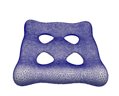
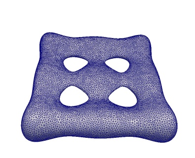
(a) $t=0.2$

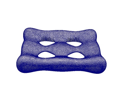
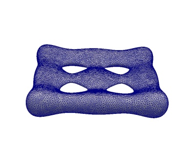
(b) $t=0.4$

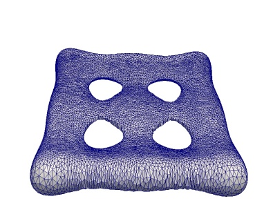
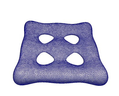
(c) $t=0.7$

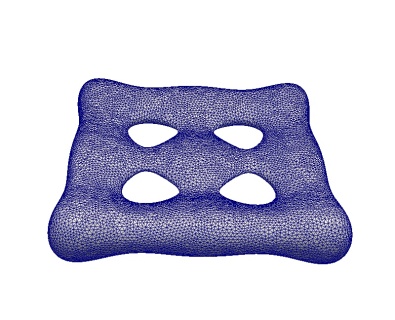
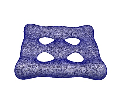
(d) $t=1$

Figure 1. Meshes obtained for Example 6.3 with an approximation of the Lagrangian (zero tangential) velocity (lefthand column) and with the ALE velocity (6.10) (righthand column).

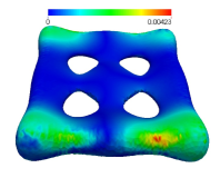
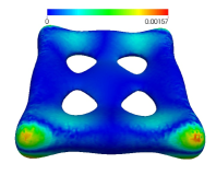
(a) $t=0.2$

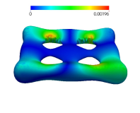
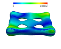
(b) $t=0.4$

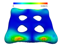
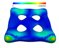
(c) $t=0.7$

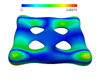
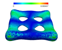
(d) $t=1$

Figure 2. Snapshots of the interpolant of the error using the two different schemes for Example 6.3, the left hand column corresponds to the Lagrangian scheme and the righthand column corresponds to the ALE scheme.

6.4 Example (Simulation on a surface with changing conormal).

We compute on a graph ${{\Gamma}(t)}$ above the unit disc which is given by the following parameterisation

(6.11) $$\boldsymbol{x}(\boldsymbol{\theta},t)=\left(\theta_{1},\theta_{2},2\sin(2\pi t)(1-\theta_{1}^{2}-\theta_{2}^{2})\right),\qquad\boldsymbol{\theta}=(\theta_{1},\theta_{2})^{T}\in B_{1}(0),t\in[0,0.25].$$

Defining the height of the graph

(6.12) $$z(\boldsymbol{\theta},t)=2\sin(2\pi t)(1-\theta_{1}^{2}-\theta_{2}^{2}),\qquad\boldsymbol{\theta}=(\theta_{1},\theta_{2})^{T}\in B_{1}(0),t\in[0,0.25],$$

we set the material velocity to be the normal velocity of the graph which is given by

(6.13) $$\boldsymbol{v}(\boldsymbol{\theta},t)=\frac{-\partial_{t}z(\boldsymbol{\theta},t)\left((\nabla z(\boldsymbol{\theta},t))^{T},-1)^{T}\right)}{1+\left|\nabla z(\boldsymbol{\theta},t)\right|^{2}},\qquad\boldsymbol{\theta}\in B_{1}(0),t\in[0,0.25].$$

We will again compare a Lagrangian and ALE scheme. For the ALE scheme we define the arbitrary velocity

(6.14) $$\boldsymbol{v}^{a}_{1}(\boldsymbol{\theta},t)=0,\boldsymbol{v}^{a}_{2}(\boldsymbol{\theta},t)=0,\boldsymbol{v}^{a}_{3}(\boldsymbol{\theta},t)=\partial_{t}z(\boldsymbol{\theta},t)\qquad\boldsymbol{\theta}\in B_{1}(0),t\in[0,0.25].$$

The arbitrary tangential velocity is then determined by $\boldsymbol{a}_{\boldsymbol{\mathcal{T}}}=\boldsymbol{v}^{a}-\boldsymbol{v}$.

For this example we define the initial triangulation ${{\Gamma}_{h}^{0}}$ (which is used for both schemes) with curved boundary faces in such a way that the initial triangulation is an exact triangulation of the unit disc, i.e., ${{\Gamma}_{h}^{0}}={\Gamma}^{0}$. We also note that as the the velocity fields $\boldsymbol{v}$ and $\boldsymbol{v}^{a}$, defined by (6.13) and (6.14) respectively, are zero on the boundary, the triangulation of the boundary remains exact for all times.

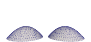
(a) $t=0.05$

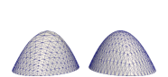
(b) $t=0.1$

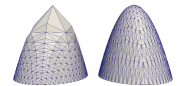
(c) $t=0.25$

Figure 3. Snapshots of the meshes obtained in Example 6.4 on moving the vertices with the Lagrangian (6.13) and ALE velocities (6.14), left and right hand meshes in each subfigure respectively, starting with the same initial triangulation with 545 vertices. We observe that moving the vertices with the Lagrangian velocity leads to a mesh that resolves the surface poorly at the final time.

In Figure 3 we show some snapshots of the evolution of the same initial triangulation using the Lagrangian and ALE velocities, we have used a coarse initial triangulation so that the individual elements are clearly visible. For this example the ALE velocity clearly yields a mesh more suitable for computation.

We consider the following equation on the surface (6.11);

(6.15) $$\partial^{\bullet}_{\boldsymbol{v}}u+u\nabla_{{{\Gamma}(t)}}\cdot\boldsymbol{v}-\Updelta_{{{\Gamma}(t)}}u=10\sin\left(2\pi x_{3}^{2}\right)\quad\mbox{ on }{{\Gamma}(t)},t\in[0,0.25],$$

with natural boundary conditions of the form (1.2). We take the initial data $u(\boldsymbol{x},0)=0$. We selected a timestep of $10^{-5}$. We employed the BDF1 (implicit Euler) scheme (5.63) to compute the discrete solutions.

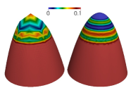
(a) Mesh with 8321 vertices

(b) Mesh with 33025 vertices

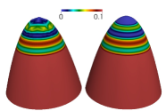
(c) Mesh with 131585 vertices

Figure 4. Snapshots of the computed solution for Example 6.4 at the end time $t=0.25$ (slightly tilted). Each subfigure shows the results of the Lagrangian (left) and ALE schemes (right) starting with the same initial triangulations for both schemes.

Figure 4 shows the computed to solution to (6.15) at the final time on successive refinements of the mesh with the ALE and Lagrangian schemes. We observe good agreement between the solutions with the coarser and finer meshes in the ALE case and qualitative agreement between these solutions and the solution with Lagrangian scheme on the finest mesh (although even with the finest mesh the resolution of the surface is poor in the Lagrangian case). On the coarser meshes the Lagrangian scheme does not adequately resolve the surface and the source term and hence generates qualitatively different solutions to the fine mesh Lagrangian and (all three) ALE simulations.

6.5 Example ( Long time Lagrangian simulations on a surface with periodic evolution ).

We consider a surface

(6.16) $${{\Gamma}(t)}=\left\{\boldsymbol{x}\in{\mathbb{R}}^{3}\left|\frac{x_{1}^{2}}{a(t)^{2}}+\frac{x_{2}^{2}}{b(t)^{2}}+\frac{x_{3}^{2}}{c(t)^{2}}-1=0\right.\right\},$$

with $a(t)=1-0.1\sin(\pi t),b(t)=1-0.2\sin(\pi t)$ and $c(t)=1+0.1\sin(\pi t)$. The surface is therefore an ellipsoid with time dependent axes and the initial surface at $t=0$ is the surface of the unit sphere. We assume the material velocity of the surface is the normal velocity. We consider (1.1) posed on the surface with four different initial conditions

(6.17) $$u_{1}(\boldsymbol{x},0) =1\quad\boldsymbol{x}\in{\Gamma}^{0},$$

(6.18) $$u_{2}(\boldsymbol{x},0) =1+\sin(2\pi x_{1})\quad\boldsymbol{x}\in{\Gamma}^{0},$$

(6.19) $$u_{3}(\boldsymbol{x},0) =1+4\sin(8\pi x_{1})+3\cos(6\pi x_{2})+2\sin(8\pi x_{3})\quad\boldsymbol{x}\in{\Gamma}^{0},$$

(6.20) $$u_{4}(\boldsymbol{x},0) =1+8\sin(16\pi x_{1})+7\cos(14\pi x_{2})+6\sin(24\pi x_{3})\quad\boldsymbol{x}\in{\Gamma}^{0}.$$

We used the Lagrangian BDF1 scheme (5.63) to simulate the equation on a triangulation of the sphere with 16386 vertices and selected a timestep of $10^{-4}$. We approximated the initial data for the numerical method as follows

(6.21) $$U_{h,1}(\boldsymbol{x},0) =1\quad\boldsymbol{x}\in{{\Gamma}_{h}^{0}},$$

(6.22) $$U_{h,2}(\boldsymbol{x},0) =\tilde{I}_{h}u_{2}(\boldsymbol{x},0)+\int_{{{\Gamma}_{h}^{0}}}\left(1-\tilde{I}_{h}u_{2}(\cdot,0)\right)\quad\boldsymbol{x}\in{{\Gamma}_{h}^{0}},$$

(6.23) $$U_{h,3}(\boldsymbol{x},0) =\tilde{I}_{h}u_{3}(\boldsymbol{x},0)+\int_{{{\Gamma}_{h}^{0}}}\left(1-\tilde{I}_{h}u_{3}(\cdot,0)\right)\quad\boldsymbol{x}\in{{\Gamma}_{h}^{0}},$$

(6.24) $$U_{h,4}(\boldsymbol{x},0) =\tilde{I}_{h}u_{4}(\boldsymbol{x},0)+\int_{{{\Gamma}_{h}^{0}}}\left(1-\tilde{I}_{h}u_{4}(\cdot,0)\right)\quad\boldsymbol{x}\in{{\Gamma}_{h}^{0}},$$

where $\tilde{I}_{h}:\operatorname{C}({\Gamma}^{0})\to{\mathcal{S}_{h}}(0)$ denotes the linear Lagrange interpolation operator. The approximations of the initial conditions for the numerical scheme were chosen such that the initial approximations have the same total mass. We note that the approximations of the the initial conditions satisfy (5.31).

Figure 5 shows plots of the initial conditions (6.22), (6.23) and (6.24) on the discrete surface. Figure 6 shows snapshots of the discrete solution for the case of constant initial data (6.21) we observe that the numerical solution appears to converge rapidly to a periodic function. We wish to investigate numerically the effect of the initial data on this periodic solution, to this end we compute the numerical solution with the initial conditions (6.22), (6.23) and (6.24) and compare these numerical solutions to that obtained with constant initial data. Figure 7 shows the $\operatorname{L}_{2}({{\Gamma}_{h}}(t))$ norm of the difference between the numerical solutions with the non-constant initial data and the numerical solution with the constant initial data versus time. It appears that the numerical solutions converge to the same periodic solution for all four different initial conditions.

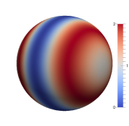
(a) $U_{h,2}(\cdot,0)$

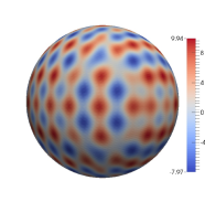
(b) $U_{h,3}(\cdot,0)$

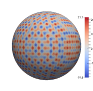
(c) $U_{h,4}(\cdot,0)$

Figure 5. Initial conditions (6.22), (6.23) and (6.24) for the simulations of Example 6.5.

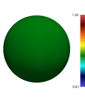
(a) $t=0$

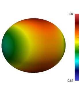
(b) $t=0.2$

(c) $t=1$

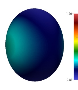
(d) $t=1.5$

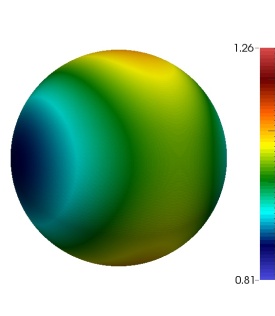
(e) $t=2$

(f) $t=2.2$

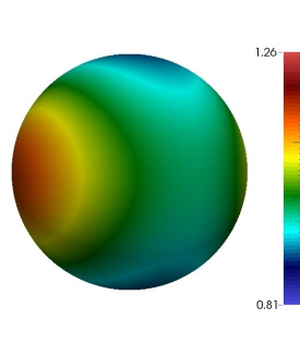
(g) $t=3$

(h) $t=3.5$

(i) $t=4$

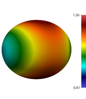
(j) $t=4.2$

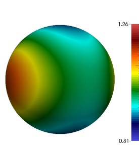
(k) $t=5$

(l) $t=5.5$

Figure 6. Snapshots of the numerical solution of Example 6.5 with constant initial data (6.21).

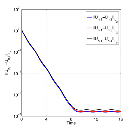
Figure 7. The $\operatorname{L}_{2}({{\Gamma}_{h}}(t))$ norm of the difference between numerical solution with constant initial data (6.21) and the numerical solutions corresponding to the initial conditions (6.22), (6.23) and (6.24) (blue, red and black lines respectively).

Appendix A Transport formula

The following transport formula play a fundamental role in the formulation and analysis of the numerical method.

A.1 Lemma (Transport formula).

Let ${\mathcal{M}}(t)$ be a smoothly evolving surface with material velocity $\boldsymbol{v}$, let $f$ and $g$ be sufficiently smooth functions and $\boldsymbol{w}$ a sufficiently smooth vector field such that all the following quantities exist. Then

(A.1) $$\frac{{\operatorname{d}}}{{\operatorname{d}}t}\int_{{\mathcal{M}}(t)}f= \int_{{\mathcal{M}}(t)}\partial^{\bullet}_{\boldsymbol{v}}f+f\nabla_{\Gamma}\cdot\boldsymbol{v},$$

(A.2) $$\frac{{\operatorname{d}}}{{\operatorname{d}}t}\int_{{\mathcal{M}}(t)}f\boldsymbol{w}\cdot\nabla_{\Gamma}g= \int_{{\mathcal{M}}(t)}\left(\partial^{\bullet}_{\boldsymbol{v}}f\boldsymbol{w}\cdot\nabla_{\Gamma}g+f\partial^{\bullet}_{\boldsymbol{v}}\boldsymbol{w}\cdot\nabla_{\Gamma}g+f\boldsymbol{w}\cdot\nabla_{\Gamma}\partial^{\bullet}_{\boldsymbol{v}}g\right)$$

$$+\int_{{\mathcal{M}}(t)}\nabla_{\Gamma}\cdot\boldsymbol{v}\left(f\boldsymbol{w}\cdot\nabla_{\Gamma}g\right)-\int_{{\mathcal{M}}(t)}f\boldsymbol{w}\cdot\mathcal{B}_{{\Gamma}}{\left(\boldsymbol{v}\right)}\nabla_{\Gamma}g$$

(A.3) $$\frac{{\operatorname{d}}}{{\operatorname{d}}t}\int_{{\mathcal{M}}(t)}\nabla_{\Gamma}f\cdot\nabla_{\Gamma}g= \int_{{\mathcal{M}}(t)}\left(\nabla_{\Gamma}\partial^{\bullet}_{\boldsymbol{v}}f\cdot\nabla_{\Gamma}g+\nabla_{\Gamma}\partial^{\bullet}_{\boldsymbol{v}}g\cdot\nabla_{\Gamma}f\right)$$

$$+\int_{{\mathcal{M}}(t)}\left(\nabla_{\Gamma}\cdot\boldsymbol{v}-2\mathcal{D}_{{\Gamma}}{\left(\boldsymbol{v}\right)}\right)\nabla_{\Gamma}f\cdot\nabla_{\Gamma}g,$$

with the deformation tensors defined by

$$\mathcal{B}_{{\Gamma}}{\left(\boldsymbol{v}_{ij}\right)}=(\nabla_{\Gamma})_{i}v_{j}-\sum_{l=1}^{m+1}\nu_{l}\nu_{i}(\nabla_{\Gamma})_{j}v_{l}\quad\text{ and }\quad\mathcal{D}_{{\Gamma}}{\left(\boldsymbol{v}_{ij}\right)}=\frac{1}{2}\left((\nabla_{\Gamma})_{i}v_{j}+(\nabla_{\Gamma})_{j}v_{i}\right),$$

respectively.

Proof . Proofs of (A.1) and (A.3) are given in [1]. The proof of (A.2) is as follows, (for further details see the proof of (A.3) in [1, Appendix]) we have

(A.4) $$\frac{{\operatorname{d}}}{{\operatorname{d}}t}\int_{{\mathcal{M}}(t)}f\boldsymbol{w}\cdot\nabla_{\Gamma}g=\int_{{\mathcal{M}}(t)}\partial^{\bullet}_{\boldsymbol{v}}\left(f\boldsymbol{w}\cdot\nabla_{\Gamma}g\right)+\nabla_{\Gamma}\cdot\boldsymbol{v}\left(f\boldsymbol{w}\cdot\nabla_{\Gamma}g\right)$$

$$=\int_{{\mathcal{M}}(t)}\bigg{(}\partial^{\bullet}_{\boldsymbol{v}}f\left(\boldsymbol{w}\cdot\nabla_{\Gamma}g\right)+f\left(\partial^{\bullet}_{\boldsymbol{v}}\boldsymbol{w}\right)\cdot\nabla_{\Gamma}g+f\boldsymbol{w}\cdot\left(\partial^{\bullet}_{\boldsymbol{v}}\nabla_{\Gamma}g\right)+\nabla_{\Gamma}\cdot\boldsymbol{v}\left(f\boldsymbol{w}\cdot\nabla_{\Gamma}g\right)\bigg{)}.$$

Finally, application of the following result from [7, Lemma 2.6]

$$\partial^{\bullet}_{\boldsymbol{v}}\nabla_{{{\Gamma}(t)}}g=\nabla_{{{\Gamma}(t)}}\partial^{\bullet}_{\boldsymbol{v}}g-\mathcal{B}_{{\Gamma}}{\left(\boldsymbol{v}\right)}\nabla_{{{\Gamma}(t)}}g,$$

in (A.4) completes the proof of the Lemma. ∎

For the analysis of the second order scheme we note that repeated application of the transport formula together with the smoothness of the velocity yields the following bounds, see [4, Lemma 9.1] for a similar discussion. Let ${\Gamma}$ be a smoothly evolving surface with material velocity $\boldsymbol{v}$, let $f$ and $g$ be sufficiently smooth functions and $\boldsymbol{w}$ a sufficiently smooth vector and further assume $\partial^{\bullet}_{\boldsymbol{v}}g=0$ then

(A.5) $$\left|\frac{{\operatorname{d}}^{2}}{{\operatorname{d}}t^{2}}\int_{{\Gamma}}\nabla_{\Gamma}f\cdot\nabla_{\Gamma}g\right| \leq\left|\int_{{\Gamma}}\nabla_{\Gamma}\partial^{\bullet}_{\boldsymbol{v}}(\partial^{\bullet}_{\boldsymbol{v}}f)\cdot\nabla_{\Gamma}g\right|$$

$$+c\left(\left|\int_{{\Gamma}}\nabla_{\Gamma}\partial^{\bullet}_{\boldsymbol{v}}f\cdot\nabla_{\Gamma}g\right|+\left|\int_{{\Gamma}}\nabla_{\Gamma}f\cdot\nabla_{\Gamma}g\right|\right),$$

(A.6) $$\left|\frac{{\operatorname{d}}^{2}}{{\operatorname{d}}t^{2}}\int_{{\Gamma}}f\boldsymbol{w}\cdot\nabla_{\Gamma}g\right| \leq\left|\int_{{\Gamma}}\partial^{\bullet}_{\boldsymbol{v}}(\partial^{\bullet}_{\boldsymbol{v}}f)\boldsymbol{w}\cdot\nabla_{\Gamma}g\right|$$

$$+c\left(\left|\int_{{\Gamma}}\partial^{\bullet}_{\boldsymbol{v}}f\boldsymbol{w}\cdot\nabla_{\Gamma}g\right|+\left|\int_{{\Gamma}}f\boldsymbol{w}\cdot\nabla_{\Gamma}g\right|\right).$$

Appendix B Approximation results

For a function $\eta\in C^{0}({{\Gamma}(t)})$ we denote by $I_{h}\eta\in{\mathcal{S}_{h}^{l}}$ the lift of the linear Lagrange interpolant of $\tilde{I}_{h}\eta\in{\mathcal{S}_{h}}$, i.e., $I_{h}\eta=(\tilde{I}_{h}\eta)^{l}$. The following Lemma was shown in [23].

B.1 Lemma (Interpolation bounds).

For an $\eta\in\operatorname{H}^{2}{{{\Gamma}(t)}}$ there exists a unique $I_{h}\eta\in{\mathcal{S}_{h}^{l}(t)}$ such that

(B.1) $$\left\|\eta-I_{h}\eta\right\|_{\operatorname{L}_{2}\left({{\Gamma}(t)}\right)}+h\left\|\nabla_{{\Gamma}(t)}(\eta-I_{h}\eta)\right\|_{\operatorname{L}_{2}\left({{\Gamma}(t)}\right)}\leq ch^{2}\left\|\eta\right\|_{\operatorname{H}^{2}({{\Gamma}(t)})}.$$

The following results provide estimates for the difference between the continuous velocity (here we mean the velocity that includes the arbitrary tangential motion and not the material velocity) and the discrete velocity of the smooth surface together with an estimate on the material derivative.

B.2 Lemma.

Velocity and material derivative estimates

(B.2) $$\left|\partial^{\bullet}_{h,\boldsymbol{v}^{a}_{h}}\left(\boldsymbol{v}_{a}-\boldsymbol{v}^{a}_{h}\right)\right|+h\left|\nabla_{{\Gamma}(t)}\partial^{\bullet}_{h,\boldsymbol{v}^{a}_{h}}\left(\boldsymbol{v}_{a}-\boldsymbol{v}^{a}_{h}\right)\right| \leq ch^{2}\quad\text{on }{\Gamma}$$

(B.3) $$\left\|\boldsymbol{a}_{\boldsymbol{\mathcal{T}}}-\boldsymbol{t}^{a}_{h}\right\|_{\operatorname{L}_{2}\left({{\Gamma}(t)}\right)}+h\left\|\nabla_{{\Gamma}(t)}\left(\boldsymbol{a}_{\boldsymbol{\mathcal{T}}}-\boldsymbol{t}^{a}_{h}\right)\right\|_{\operatorname{L}_{2}\left({{\Gamma}(t)}\right)} \leq ch^{2}\left\|\boldsymbol{a}_{\boldsymbol{\mathcal{T}}}\right\|_{\operatorname{H}^{2}({{\Gamma}(t)})}.$$

(B.4) $$\left\|\partial^{\bullet}_{\boldsymbol{v}_{a}}z-\partial^{\bullet}_{h,\boldsymbol{v}^{a}_{h}}z\right\|_{\operatorname{L}_{2}\left({{\Gamma}(t)}\right)} \leq ch^{2}\left\|z\right\|_{\operatorname{H}^{1}({{\Gamma}(t)})}$$

(B.5) $$\left\|\nabla_{{\Gamma}(t)}\left(\partial^{\bullet}_{\boldsymbol{v}_{a}}z-\partial^{\bullet}_{h,\boldsymbol{v}^{a}_{h}}z\right)\right\|_{\operatorname{L}_{2}\left({{\Gamma}(t)}\right)} \leq ch\left\|z\right\|_{\operatorname{H}^{2}({{\Gamma}(t)})}$$

(B.6) $$\left\|\partial^{\bullet}_{\boldsymbol{v}_{a}}\partial^{\bullet}_{\boldsymbol{v}_{a}}z-\partial^{\bullet}_{\boldsymbol{v}^{a}_{h}}\partial^{\bullet}_{h,\boldsymbol{v}^{a}_{h}}z\right\|_{\operatorname{L}_{2}\left({{\Gamma}(t)}\right)} \leq ch^{2}\left\|\partial^{\bullet}_{\boldsymbol{v}}z\right\|_{\operatorname{H}^{1}({{\Gamma}(t)})}$$

(B.7) $$\left\|\nabla_{{\Gamma}(t)}\left(\partial^{\bullet}_{\boldsymbol{v}_{a}}\partial^{\bullet}_{\boldsymbol{v}_{a}}z-\partial^{\bullet}_{\boldsymbol{v}^{a}_{h}}\partial^{\bullet}_{h,\boldsymbol{v}^{a}_{h}}z\right)\right\|_{\operatorname{L}_{2}\left({{\Gamma}(t)}\right)} \leq ch\left\|\partial^{\bullet}_{\boldsymbol{v}}z\right\|_{\operatorname{H}^{2}({{\Gamma}(t)})}.$$

Proof . The estimate (B.2) is shown in [8, Lemma 7.3], (B.3) follows from Lemma B.1 and the fact that $\boldsymbol{T}^{a}_{h}$ is the interpolant of the arbitrary tangential velocity and $\boldsymbol{t}^{a}_{h}$ is its lift. Estimates (B.4) and (B.5) are shown in [2, Cor. 5.7]. The estimates (B.6) and (B.7) follow easily from (B.2), (B.4) and (B.5). ∎

We now state some results on the error due to the approximation of the surface

B.3 Lemma (Geometric perturbation errors).

For any $(\Psi_{h}(\cdot,t),\Phi_{h}(\cdot,t))\in{\mathcal{S}_{h}}(t)\times{\mathcal{S}_{h}}(t)$ with corresponding lifts $(\psi_{h}(\cdot,t),\varphi_{h}(\cdot,t))\in{\mathcal{S}_{h}^{l}}(t)\times{\mathcal{S}_{h}^{l}}(t),$ the following bounds hold:

(B.8) $$\left|m\left({\psi_{h}},{\varphi_{h}}\right)-m_{h}\left({\Psi_{h}},{\Phi_{h}}\right)\right| \leq ch^{2}\left\|\psi_{h}\right\|_{\operatorname{L}_{2}\left({{\Gamma}(t)}\right)}\left\|\varphi_{h}\right\|_{\operatorname{L}_{2}\left({{\Gamma}(t)}\right)}$$

(B.9) $$\left|a\left({\psi_{h}},{\varphi_{h}}\right)-a_{h}\left({\Psi_{h}},{\Phi_{h}}\right)\right| \leq ch^{2}\left\|\nabla_{{{\Gamma}(t)}}\psi_{h}\right\|_{\operatorname{L}_{2}\left({{\Gamma}(t)}\right)}\left\|\nabla_{{{\Gamma}(t)}}\varphi_{h}\right\|_{\operatorname{L}_{2}\left({{\Gamma}(t)}\right)}$$

(B.10) $$\left|g\left({\psi_{h}},{\varphi_{h}};{\boldsymbol{v}^{a}_{h}}\right)-g_{h}\left({\Psi_{h}},{\Phi_{h}};{\boldsymbol{V}^{a}_{h}}\right)\right| \leq ch^{2}\left\|\psi_{h}\right\|_{\operatorname{H}^{1}({{\Gamma}(t)})}\left\|\varphi_{h}\right\|_{\operatorname{H}^{1}({{\Gamma}(t)})}$$

(B.11) $$\left|b\left({\psi_{h}},{\varphi_{h}};{\boldsymbol{t}^{a}_{h}}\right)-b_{h}\left({\Psi_{h}},{\Phi_{h}};{\boldsymbol{T}^{a}_{h}}\right)\right| \leq ch^{2}\left\|\psi_{h}\right\|_{\operatorname{L}_{2}\left({{\Gamma}(t)}\right)}\left\|\nabla_{{\Gamma}(t)}\varphi_{h}\right\|_{\operatorname{L}_{2}\left({{\Gamma}(t)}\right)},$$

with $\boldsymbol{V}^{a}_{h},\boldsymbol{T}^{a}_{h},\boldsymbol{v}^{a}_{h}$ and $\boldsymbol{t}^{a}_{h}$ as defined in §3.

Proof . A proof of (B.8), (B.9) and (B.10) is given in [2, Lemma 5.5]. We now prove (B.11). We start by introducing some notation. We denote by $\delta_{h}$ the quotient between the discrete and smooth surface measures which satisfies [1, Lemma 5.1]

(B.12) $$\sup_{t\in(0,T)}\sup_{{{\Gamma}_{h}(t)}}\left|1-\delta_{h}\right|\leq ch^{2}$$

We introduce $\boldsymbol{P},\boldsymbol{P}_{h}$ the projections onto the tangent planes of ${{\Gamma}(t)}$ and ${{\Gamma}_{h}}$ respectively. We denote by ${\boldsymbol{\mathcal{H}}}$ the Weingarten map $(\mathcal{H}_{ij}=\partial_{x_{j}}\nu_{i})$.

(B.13) $$\left|b\left({\psi_{h}},{\varphi_{h}};{\boldsymbol{t}^{a}_{h}}\right)-b_{h}\left({\Psi_{h}},{\Phi_{h}};{\boldsymbol{T}^{a}_{h}}\right)\right|=\left|\int_{{\Gamma}(t)}\psi_{h}\boldsymbol{t}^{a}_{h}\cdot\nabla_{{\Gamma}(t)}\varphi_{h}-\int_{{{\Gamma}_{h}(t)}}\Psi_{h}\boldsymbol{T}^{a}_{h}\cdot\nabla_{{\Gamma}_{h}(t)}\Phi_{h}\right|$$

From [1] we have

(B.14) $$\nabla_{{\Gamma}_{h}}\eta=\boldsymbol{B}_{h}\nabla_{\Gamma}\eta^{l},$$

where $\boldsymbol{B}_{h}=\boldsymbol{P}_{h}(\boldsymbol{I}-d\boldsymbol{\mathcal{H}})$. We have with $\boldsymbol{p},\boldsymbol{x}$ as in (3.1),

(B.15) $$\boldsymbol{T}^{a}_{h}(\boldsymbol{x},\cdot)\cdot\nabla_{{\Gamma}_{h}}\Phi_{h}(\boldsymbol{x},\cdot) =\boldsymbol{P}_{h}\boldsymbol{T}^{a}_{h}(\boldsymbol{x},\cdot)\cdot\nabla_{{\Gamma}_{h}}\Phi_{h}(\boldsymbol{x},\cdot)$$

$$=\boldsymbol{P}_{h}\boldsymbol{t}^{a}_{h}(\boldsymbol{p},\cdot)\cdot\boldsymbol{P}_{h}(\boldsymbol{I}-d\boldsymbol{\mathcal{H}})\boldsymbol{P}\nabla_{\Gamma}\varphi_{h}(\boldsymbol{p},\cdot)$$

$$=\boldsymbol{P}_{h}\boldsymbol{t}^{a}_{h}(\boldsymbol{p},\cdot)\cdot\boldsymbol{P}_{h}\boldsymbol{P}(\boldsymbol{I}-d\boldsymbol{\mathcal{H}})\nabla_{\Gamma}\varphi_{h}(\boldsymbol{p},\cdot)$$

$$=(\boldsymbol{I}-d\boldsymbol{\mathcal{H}})\boldsymbol{P}\boldsymbol{P}_{h}\boldsymbol{t}^{a}_{h}(\boldsymbol{p},\cdot)\cdot\nabla_{\Gamma}\varphi_{h}(\boldsymbol{p},\cdot)$$

$$={\boldsymbol{\mathcal{Q}}_{h}}\boldsymbol{t}^{a}_{h}(\boldsymbol{p},\cdot)\cdot\nabla_{\Gamma}\varphi_{h}(\boldsymbol{p},\cdot)$$

where the last equality defines $\boldsymbol{\mathcal{Q}}_{h}$. We denote the lifted version by $\boldsymbol{\mathcal{Q}}_{h}^{l}$ Thus we may write (B.13) as

(B.16) $$\left|b\left({\psi_{h}},{\varphi_{h}};{\boldsymbol{t}^{a}_{h}}\right)-b_{h}\left({\Psi_{h}},{\Phi_{h}};{\boldsymbol{T}^{a}_{h}}\right)\right| =\left|\int_{{\Gamma}(t)}\psi_{h}\boldsymbol{t}^{a}_{h}\cdot\nabla_{{\Gamma}(t)}\varphi_{h}-\int_{{\Gamma}(t)}\frac{1}{\delta_{h}^{l}}\psi_{h}\boldsymbol{\mathcal{Q}}^{l}_{h}\boldsymbol{t}^{a}_{h}\cdot\nabla_{{\Gamma}(t)}\varphi_{h}\right|$$

$$\leq\left|\int_{{\Gamma}(t)}\psi_{h}(\boldsymbol{I}-\boldsymbol{\mathcal{Q}}^{l}_{h})\boldsymbol{P}\boldsymbol{t}^{a}_{h}\cdot\nabla_{{\Gamma}(t)}\varphi_{h}\right|+ch^{2},$$

where we have used (B.12). We now apply the following result from [1, Lem 5.1]

(B.17) $$\sup_{t\in(0,T)}\sup_{{{\Gamma}_{h}(t)}}\left|\left(\boldsymbol{I}-\boldsymbol{\mathcal{Q}}_{h}\right)\boldsymbol{P}\right|\leq ch^{2},$$

which yields the desired bound. ∎

Appendix C Ritz projection estimates

It proves helpful in the analysis to introduce the Ritz projection $\operatorname{R}^{h}:\operatorname{H}^{1}({\Gamma})\to{\mathcal{S}_{h}^{l}}$ defined as follows: for $z\in\operatorname{H}^{1}({\Gamma})$ with $\int_{\Gamma}z=0$,

(C.1) $$a\left({\operatorname{R}^{h}z},{\varphi_{h}}\right)=a\left({z},{\varphi_{h}}\right)\quad\forall\varphi_{h}\in{\mathcal{S}_{h}^{l}},$$

with $\int_{\Gamma}\operatorname{R}^{h}z=0$.

C.1 Lemma (Ritz projection estimates).

We recall the following estimates proved in [2, Thm. 6.1 and Thm. 6.2] that hold for the mesh-size $h$ sufficiently small

(C.2) $$\left\|z-\operatorname{R}^{h}z\right\|_{\operatorname{L}_{2}\left({\Gamma}\right)} +h\left\|\nabla_{\Gamma}\left(z-\operatorname{R}^{h}z\right)\right\|_{\operatorname{L}_{2}\left({\Gamma}\right)}\leq ch^{2}\left\|z\right\|_{\operatorname{H}^{2}({\Gamma})}.$$

(C.3) $$\left\|\partial^{\bullet}_{h,\boldsymbol{v}^{a}_{h}}\left(z-\operatorname{R}^{h}z\right)\right\|_{\operatorname{L}_{2}\left({\Gamma}\right)} +h\left\|\nabla_{\Gamma}\partial^{\bullet}_{h,\boldsymbol{v}^{a}_{h}}\left(z-\operatorname{R}^{h}z\right)\right\|_{\operatorname{L}_{2}\left({\Gamma}\right)}\leq$$

$$ch^{2}\left(\left\|z\right\|_{\operatorname{H}^{2}({\Gamma})}+\left\|\partial^{\bullet}_{\boldsymbol{v}_{a}}z\right\|_{\operatorname{H}^{2}({\Gamma})}\right).$$

References

- Dziuk and Elliott [2007] G. Dziuk and C. M. Elliott. Finite elements on evolving surfaces. IMA Journal of Numerical Analysis, 27(2):262, 2007.
- Dziuk and Elliott [2013a] G. Dziuk and C. M. Elliott. L2-estimates for the evolving surface finite element method. Mathematics of Computation, 82(281):1–24, 2013.
- Dziuk and Elliott [2012] G. Dziuk and C. M. Elliott. A fully discrete evolving surface finite element method. SIAM Journal on Numerical Analysis, 50(5):2677–2694, 2012. doi: 10.1137/110828642. URL http://epubs.siam.org/doi/abs/10.1137/110828642.
- Dziuk et al. [2012] G. Dziuk, Ch. Lubich, and D. Mansour. Runge–Kutta time discretization of parabolic differential equations on evolving surfaces. IMA Journal of Numerical Analysis, 32(2):394–416, 2012.
- Lubich et al. [2013] Ch. Lubich, D. Mansour, and C. Venkataraman. Backward difference time discretization of parabolic differential equations on evolving surfaces. IMA Journal of Numerical Analysis, 33(4):1365–1385, 2013.
- Elliott and Ranner [2013] C. M. Elliott and T. Ranner. Evolving surface finite element method for the Cahn-Hilliard equation. Numerische Mathematik, 1-52, 2014. doi: 10.1007/s00211-014-0644-y. URL http://dx.doi.org/10.1007/s00211-014-0644-y.
- Dziuk et al. [2013] G. Dziuk, D. Kröner, and T. Müller. Scalar conservation laws on moving hypersurfaces. Interfaces and Free Boundaries, 15(2):203–236, 2013.
- Lubich and Mansour [2014] Ch. Lubich and D. Mansour. Variational discretization of linear wave equations on evolving surfaces. Mathematics of Computation (In Press), 2014.
- Dziuk and Elliott [2013b] G. Dziuk and C. M. Elliott. Finite element methods for surface PDEs. Acta Numerica, 22:289–396, 2013b.
- Elliott and Styles [2012] C. M. Elliott and V. Styles. An ALE-ESFEM for solving PDEs on evolving surfaces. Milan Journal of Mathematics, 80:469–501, 2012. ISSN 1424-9286. doi: 10.1007/s00032-012-0195-6. URL http://dx.doi.org/10.1007/s00032-012-0195-6.
- Neilson et al. [2010] M. P. Neilson, J. A. Mackenzie, S. D. Webb, and R. H. Insall. Use of the parameterised finite element method to robustly and efficiently evolve the edge of a moving cell. Integrative Biology, 2(11-12):687–695, 2010.
- Elliott and Stinner [2012] C. M. Elliott and Björn Stinner. Computation of two-phase biomembranes with phase dependent material parameters using surface finite elements. Communications in Computational Physics, 13(2):325–360, 2012.
- Croft et al. [2013] W. Croft, C. M. Elliott, G. Ladds, B. Stinner, C. Venkataraman, and C. Weston. Parameter identification problems in the modelling of cell motility. Journal of Mathematical Biology (In Press), 2014.
- Elliott et al. [2012] C. M. Elliott, B. Stinner, and C. Venkataraman. Modelling cell motility and chemotaxis with evolving surface finite elements. Journal of The Royal Society Interface, 9(76):3027–3044, 2012. doi: 10.1098/rsif.2012.0276. URL http://rsif.royalsocietypublishing.org/content/9/76/3027.abstract.
- Vierling [2011] M. Vierling. Parabolic optimal control problems on evolving surfaces subject to point-wise box constraints on the control - theory and numerical realization. Interfaces and Free Boundaries, 16(2):137–173, 2014.
- Olshanskii et al. [2013] M. A. Olshanskii, A. Reusken, and X. Xu. An Eulerian space-time finite element method for diffusion problems on evolving surfaces. SIAM Journal on Numerical Analysis, 52(3), 2014.
- [17] A. Alphonse, C. M. Elliott, and B. Stinner. An abstract framework for parabolic PDEs on evolving spaces. arXiv preprint arXiv:1403.4500, 2014.
- Elliott and Stuart [1993] C. M. Elliott and A.M. Stuart. The global dynamics of discrete semilinear parabolic equations. SIAM Journal on Numerical Analysis, 30(6):1622–1663, 1993.
- Brenner and Scott [2002] S.C. Brenner and L.R. Scott. The mathematical theory of finite element methods. Texts in Applied Mathematics, vol. 15, Springer, 2002.
- Schmidt and Siebert [2005] A. Schmidt and K.G. Siebert. Design of adaptive finite element software: The finite element toolbox ALBERTA. Springer Verlag, 2005.
- Henderson et al. [2004] A. Henderson, J. Ahrens, and C. Law. The ParaView Guide. Kitware Clifton Park, NY, 2004.
- Rineau and Yvinec [2013] L. Rineau and M. Yvinec. 3D surface mesh generation. In CGAL User and Reference Manual. CGAL Editorial Board, 4.3 edition, 2013. URL http://doc.cgal.org/4.3/Manual/packages.html#PkgSurfaceMesher3Summary.
- Dziuk [1988] G. Dziuk. Finite elements for the Beltrami operator on arbitrary surfaces. Partial Differential Equations and Calculus of Variations, Lecture Notes Math 1357:142-155, Berlin Heidelberg New York: Springer 1988.