Precision measurements with photon-subtracted or photon-added Gaussian states

Abstract

Photon-subtracted and photon-added Gaussian states are amongst the simplest non-Gaussian states that are experimentally available. It is generally believed that they are some of the best candidates to enhance sensitivity in parameter extraction. We derive here the quantum Cramér-Rao bound for such states and find that for large photon numbers photon-subtraction or -addition only leads to a small correction of the quantum Fisher information (QFI). On the other hand a divergence of the QFI appears for very small squeezing in the limit of vanishing photon number in the case of photon subtraction, implying an arbitrarily precise measurement with almost no light. However, at least for the standard and experimentally established preparation scheme, the decreasing success probability of the preparation in that limit exactly cancels the divergence, leading to finite sensitivity per square root of Hertz, when the duration of the preparation is taken into account.

I Introduction

Propelled by the perspective of quantum information applications, the creation and use of non-classical states of light has seen a large increase of interest in recent years. Classical light is often understood as light which allows a description through a well-defined positive $P$-function, whereas all other states are called non-classical Kim et al. (2005); Mandel (1986). But different classes of non-classical quantum states can be considered.

A first category are squeezed Gaussian states Hudson (1974); Soto and Claverie (1983); Mandilara et al. (2009). Gaussian states include a large variety of experimentally relevant states that can be produced with high photon numbers, such as coherent states, single- or multi-mode squeezed states (and therefore entangled states), and thermal states. Combining squeezed vacuum with a bright coherent state on a beam-splitter is an important experimental tool for achieving highly sensitive measurements Caves (1981); Keller et al. (2008); Abadie et al. (2011).

As second category which is relevant for quantum information is the class of states whose Wigner function is not positive everywhere. For brevity we call such states negative Wigner function states. This type of non-classicality is motivated amongst other things by the continuous variable version of the Gottesmann-Knill theorem which states that universal quantum computation with continuous variables requires Hamiltonians that are at least cubic in the quadrature operators Braunstein and van Loock (2005). Moreover, it was recently shown that quantum algorithms for which both the initial state and the following operations can be represented by positive Wigner functions can be simulated efficiently on a classical computer Mari and Eisert (2012).

One of the most promising approaches to negative Wigner function states of light is through photon subtraction or addition. Proposed theoretically at the end of last century Dakna et al. (1997), photon subtraction from a coherent state of light was realized experimentally by Grangier et al. in 2004 Wenger et al. (2004). Since then a multitude of extensions have been found or proposed, including photon addition, multiple photon subtraction, coherent superposition of addition and subtraction of photons, or subtraction from more general states of light (see Kim (2008); Neergaard-Nielsen et al. (2011) and references therein). This kind of non-classical light can be used for increasing entanglement and consequently efficiency of quantum teleportation protocols, for the demonstration of non-locality and loophole-free violation of Bell’s inequalities, for generating Schrödinger kitten states, for quantum computing, for noise-less probabilistic amplification, and for the experimental verification of the bosonic commutation relations Ourjoumtsev et al. (2007); Lee et al. (2011); Navarrete-Benlloch et al. (2012); Ferreyrol et al. (2010); Xiang et al. (2010); Bimbard et al. (2010); Zavatta et al. (2009); Takahashi et al. (2008); Gerrits et al. (2010); Nha and Carmichael (2004); García-Patrón et al. (2004); Dakna et al. (1997); Parigi et al. (2007); Bartley et al. (2013); Lee et al. (2013); Kim et al. (2012); Kim (2008); Neergaard-Nielsen et al. (2011).

The ultimate sensitivity limits of quantum parameter estimation with Gaussian states, both pure and mixed, and the multi-parameter limits for the single-mode case, are now fully understood Pinel et al. (2012, 2013); Monras (2013). As long as the parameter to be estimated does not depend on the number of photon itself, Gaussian states always lead to a best scaling as $1/\sqrt{N}$ with the average photon number $N$. However, the prefactor depends on the squeezing. In Pinel et al. (2012) the optimal measurement strategy was identified for finite squeezing resources which makes use of a specific detection mode.

So far it was unknown if the relatively simple procedure of subtracting (or adding) photons from (or to) Gaussian states can substantially enhance the sensitivity with which certain parameters coded in the state of light can be measured, and in particular if it is possible to beat the standard quantum limit (SQL) this way. The latter corresponds to the sensitivity achievable with a coherent state and is characterized by a $1/\sqrt{N}$ scaling of the sensitivity with the mean photon number $N$ (see e.g. Giovannetti et al. (2004)).

In this paper we provide an answer to this question by calculating the quantum Cramér-Rao bound for the sensitivity with which a parameter characterizing the original Gaussian state can be measured after addition or subtraction of a photon. We show that for large photon numbers $N$ single photon-subtraction or -addition only leads to a correction of order $1/N$ of the quantum Fisher information (QFI). Surprisingly, however, a divergence of the QFI appears for very small squeezing in the limit of vanishing photon number in the case of photon subtraction, implying an arbitrary precise measurement with almost no light. However, at least for the standard and experimentally established preparation scheme, the decreasing success probability of the preparation in that limit exactly cancels the divergence, leading to finite sensitivity per square root of Hertz, when the duration of the preparation is taken into account. Nevertheless, these results may find application in niches where precise measurements are required with almost no light, as for example in the context of biological samples Wolfgramm et al. (2012).

II Photon subtraction and addition

Different approaches to photon-subtracted states are found in the literature. Kim et al. Kim et al. (2005) consider a physical process of photon-subtraction close to the experimental procedure Wenger et al. (2004), where the original state consists of squeezed vacuum that passes a beam splitter. Single photon detection is implemented in one output mode, and the detection of a single photon in that mode heralds a photon-subtracted state in the other output mode, whose properties can be verified with standard Wigner-function reconstruction techniques. This approach allowed Kim et al. to take into account losses and analyze conditions for observing the negativity of the Wigner function.

We take a simpler approach, following Kim et al. (2012), and define a photon-subtracted state relative to a reference state $\hat{\rho}$ in the single mode case by

$$\hat{\rho}^{-}=\hat{a}\hat{\rho}\hat{a}^{\dagger}/N^{-}\,$$ (1)

where $\hat{a}$ is the photon annihilation operator, $\hat{a}^{\dagger}$ is the photon creation operator, and $N^{-}={\rm tr}(\hat{a}^{\dagger}\hat{a}\hat{\rho})=N$ is the mean photon number. A photon-added state is defined correspondingly as

$$\hat{\rho}^{+}=\hat{a}^{\dagger}\hat{\rho}\hat{a}/N^{+}\,,$$ (2)

with $N^{+}={\rm tr}(\hat{a}\hat{a}^{\dagger}\hat{\rho})=N+1$. This definition immediately implies that a single coherent state $|\alpha\rangle$ is invariant under photon subtraction, but not under photon addition. We will come back to the question of state preparation and its impact on the experimentally relevant sensitivities in Sec. IV.2

The Wigner function of a single mode state $\hat{\rho}$ as function of the quadratures $x$ and $p$ is defined as Gardiner and Zoller (2004); Schleich (2011)

$$W(x,p)[\hat{\rho}]=\frac{1}{\pi}\int dy\langle x+y|\hat{\rho}|x-y\rangle e^{-2iyp}\,.$$ (3)

Here and in the following we set $\hbar=1$, such that $\hat{x}=(\hat{a}+\hat{a}^{\dagger})/\sqrt{2}$ and $\hat{p}=i(\hat{p}-\hat{x})/\sqrt{2}$. States $\hat{x}\hat{\rho}$, $\hat{p}\hat{\rho}$, etc., then have Wigner functions (see Eq. (4.5.11) in Gardiner and Zoller (2004))

$$W(x,p)[\hat{x}\hat{\rho}] = \left(x+\frac{i}{2}\partial_{p}\right)W(x,p)[\hat{\rho}]$$ (4)

$$W(x,p)[\hat{\rho}\hat{x}] = \left(x-\frac{i}{2}\partial_{p}\right)W(x,p)[\hat{\rho}]$$ (5)

$$W(x,p)[\hat{p}\hat{\rho}] = \left(p-\frac{i}{2}\partial_{x}\right)W(x,p)[\hat{\rho}]$$ (6)

$$W(x,p)[\hat{\rho}\hat{p}] = \left(p+\frac{i}{2}\partial_{x}\right)W(x,p)[\hat{\rho}]\,.$$ (7)

The general $M$-mode case is obtained in a completely analogous fashion by simply replacing the single quadratures $x,p$ with a vector ${\mathbf{X}}^{t}=(x_{1},p_{1},\ldots,x_{M},p_{M})$, and adding a label for mode $k$ in which the photon is added/subtracted. We write the corresponding density matrix as $\hat{\rho}^{(\pm,k)}$. Combining the definitions of $\hat{a}$, $\hat{a}^{\dagger}$ with Eq. (1), Eq. (2), and Eqs. (4-7), we find for the Wigner function

$$W({\mathbf{X}})[\hat{\rho}^{(\pm,k)}]=\frac{1}{2}\left(x_{k}^{2}+p_{k}^{2}\mp x_{k}\partial_{x_{k}}\mp p_{k}\partial_{p_{k}}+\frac{1}{4}(\partial_{p_{k}}^{2}+\partial_{x_{k}}^{2})+1\right)W({\mathbf{X}})[\hat{\rho}]/N^{\pm}\,.$$ (8)

III Quantum Cramér-Rao bound

Quantum parameter estimation theory (QPET) establishes the ultimate lower bound to the sensitivity with which a classical parameter $\theta$ that parametrizes the quantum state can be measured. This sensitivity is fundamentally due to quantum fluctuations, and becomes relevant once all other sources of noise, error and imperfection are eliminated. QPET generalizes classical parameter estimation theory (PET), which sets a lower bound on the fluctuations with which a parameter characterizing a probability distribution $p(\theta,A)$ of measurement outcomes $A_{i}$ of an observable $A$ can be estimated. It is optimized over all possible estimator functions Rao (1945); Cramér (1999). QPET gives the additional freedom to optimize over all possible (POVM-)measurements Braunstein and Caves (1994) that generate the probability distributions $p(\theta,A)$. Performing that optimization, one finds that the standard deviation $\delta\theta$ of the fluctuations of $\theta$ estimated from $Q$ measurements are bounded from below by the quantum Cramér-Rao bound (QCRB)

$$\delta\theta\geq\delta\theta_{\rm min}\equiv\frac{1}{\sqrt{QI(\hat{\rho}(\theta))}}\,,$$ (9)

where $I(\hat{\rho}(\theta))=\sqrt{2d_{\rm Bures}(\hat{\rho}(\theta),\hat{\rho}(\theta+d\theta))}$ is the Bures distance between $\hat{\rho}(\theta)$ and $\hat{\rho}(\theta+d\theta)$ (also called quantum Fisher information), defined as $d_{\rm Bures}(\hat{\rho}_{1},\hat{\rho}_{2})=\sqrt{2}\sqrt{1-\sqrt{F(\hat{\rho}_{1},\hat{\rho}_{2})}}$ through the fidelity $F(\hat{\rho}_{1},\hat{\rho}_{2})={\rm tr}(\hat{\rho}_{1}^{1/2}\hat{\rho}_{2}\hat{\rho}_{1}^{1/2})$. For pure states the fidelity reduces to the squared overlap of the two states, $F(|\psi\rangle\langle\psi|,|\phi\rangle\langle\phi|)=|\langle\psi|\phi\rangle|^{2}$.

In Pinel et al. (2012) we gave the formula for the Fisher information for an arbitrary pure state described in terms of its Wigner function. With Eq. (8), we therefore have the general translation of the change of sensitivity from any pure state, whose Wigner function we know, to a state where a single photon is subtracted or added in mode $k$. In terms of the Fisher information,

$$I(\hat{\rho}^{(\pm,k)}(\theta))=2(2\pi)^{M}\int_{-\infty}^{\infty}\left(W({\mathbf{X}})^{\prime}[\hat{\rho}^{(\pm,k)}]\right)^{2}d{\mathbf{X}}^{2M}\,,$$ (10)

where the ^′ means differentiation with respect to $\theta$, the integral over $d{\mathbf{X}}=dx_{1}\,dp_{1}\ldots dx_{M}\,dp_{M}$ is over all modes, and we have corrected for a factor 2 due to a different convention for the quadratures in Pinel et al. (2012). Note that $N^{\pm}$ will, in general, also depend on $\theta$.

IV QCR for single-photon-subtracted Gaussian states

In the following we restrict ourselves to the single mode case and therefore drop the index $k$. We assume that the co-variance matrix takes a diagonal form and we write $\mbox{\boldmath{$\Gamma$}}={\rm diag}(\Gamma_{xx},\Gamma_{pp})$ with $(\Gamma_{xx})^{-1}=2\langle(\hat{x}-\langle\hat{x}\rangle)^{2}\rangle$ and $(\Gamma_{pp})^{-1}=2\langle(\hat{p}-\langle\hat{p}\rangle)^{2}\rangle$. This can always be achieved by choosing an appropriate linear combination of the quadratures $x$ and $p$. We do not consider the case where the rotation depends on the parameter $\theta$. Introducing the $\theta$ dependence, the Wigner function of a Gaussian state is then given by

$$W_{\theta}(x,p)[\hat{\rho}]=\frac{\sqrt{\Gamma_{xx,\theta}\Gamma_{pp,\theta}}}{\pi}e^{-(x-\overline{x}_{\theta})^{2}\Gamma_{xx,\theta}-(p-\overline{p}_{\theta})^{2}\Gamma_{pp,\theta}}\,,$$ (11)

where the subscripts $\theta$ indicate the parameter dependence of the average values of the quadratures and of the inverse covariance matrix. We specialize on pure states for all values of $\theta$, in which case one has $\Gamma_{xx,\theta}\Gamma_{pp,\theta}=1$. Thus, we are led to the final form of the Wigner function of a pure Gaussian single-mode state

$$W_{\theta}(x,p)[\hat{\rho}]=\frac{1}{\pi}e^{-(x-\overline{x}_{\theta})^{2}\Gamma_{\theta}-(p-\overline{p}_{\theta})^{2}/\Gamma_{\theta}}\,,$$ (12)

where we have abbreviated $\Gamma_{\theta}\equiv\Gamma_{xx,\theta}$. For $\Gamma_{\theta}=1$, this is a coherent state, otherwise a pure squeezed state. For reference below we note the Fisher information for a pure Gaussian state with Wigner function given by Eq. (12) Pinel et al. (2012)

$$I_{G} = \frac{4\Gamma_{\theta}\overline{p}_{\theta}^{\prime 2}+4\Gamma_{\theta}^{3}\overline{x}_{\theta}^{\prime 2}+\Gamma_{\theta}^{\prime 2}}{2\Gamma_{\theta}^{2}}\,.$$ (13)

For a coherent state, this reduces to

$$I_{\rm coher}=2(\overline{x}_{\theta}^{\prime 2}+\overline{p}_{\theta}^{\prime 2})\,.$$ (14)

IV.1 General result

Inserting Eq. (12) into Eq. (8) we find the explicit Wigner function of the photon-subtracted single-mode Gaussian state

$$W_{\theta}(x,p)[\hat{\rho}^{-}] = \frac{e^{-\frac{(p-\overline{p}_{\theta})^{2}}{\Gamma_{\theta}}-(x-\overline{x}_{\theta})^{2}\Gamma_{\theta}}}{\pi\Gamma_{\theta}^{2}\left(2\left(-1+\overline{p}_{\theta}^{2}+\overline{x}_{\theta}^{2}\right)+\frac{1}{\Gamma_{\theta}}+\Gamma_{\theta}\right)}\big{(}2p^{2}+2\overline{p}_{\theta}^{2}+4p\overline{p}_{\theta}(-1+\Gamma_{\theta})$$

$$-\left(1+4p^{2}\right)\Gamma_{\theta}+2\left(1+p^{2}+x^{2}\right)\Gamma_{\theta}^{2}+\left(-1-4x^{2}+4x\overline{x}_{\theta}\right)\Gamma_{\theta}^{3}+2(x-\overline{x}_{\theta})^{2}\Gamma_{\theta}^{4}\big{)}\,.$$

The Wigner-function for a photon-subtracted state is plotted in Fig. 1. We see that photon subtraction leads to a large “hole” where the Wigner-function becomes negative, confirming the strongly non-classical character of such a state. One checks that for $\Gamma_{\theta}=1$, Eq. (IV.1) gives back Eq. (12), confirming the invariance of a coherent state under photon-subtraction.

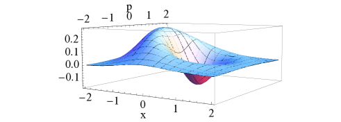
Figure 1: Wigner function of photon-subtracted state for $\Gamma_{\theta}=1.1$, $\overline{x}_{\theta}=1/20$.

The squared term in Eq. (10) can still be evaluated analytically. We find that the Fisher information is given by

$$I(\hat{\rho}^{(-)}(\theta)) = \frac{1}{2\left(\Gamma_{\theta}+2\left(-1+\overline{p}_{\theta}^{2}+\overline{x}_{\theta}^{2}\right)\Gamma_{\theta}^{2}+\Gamma_{\theta}^{3}\right)^{2}}$$ (16)

$$\times\Big{\{}4\Gamma_{\theta}(3+\Gamma_{\theta}(-8+8\overline{p}_{\theta}^{2}+10\Gamma_{\theta}$$

$$+4\left(-2+\overline{p}_{\theta}^{2}+\overline{x}_{\theta}^{2}\right)\left(\overline{p}_{\theta}^{2}+\overline{x}_{\theta}^{2}\right)\Gamma_{\theta}+8\left(-1+\overline{x}_{\theta}^{2}\right)\Gamma_{\theta}^{2}+3\Gamma_{\theta}^{3}))\left(\overline{p}_{\theta}^{\prime 2}+\Gamma_{\theta}^{2}\overline{x}_{\theta}^{\prime 2}\right)$$

$$+32\Gamma_{\theta}^{2}(\overline{p}_{\theta}\left(1+\left(-1+\overline{p}_{\theta}^{2}+\overline{x}_{\theta}^{2}\right)\Gamma_{\theta}\right)\overline{p}_{\theta}^{\prime}-\overline{x}_{\theta}\Gamma_{\theta}\left(-1+\overline{p}_{\theta}^{2}+\overline{x}_{\theta}^{2}+\Gamma_{\theta}\right)\overline{x}_{\theta}^{\prime})\Gamma_{\theta}^{\prime}$$

$$+\Big{(}3+\Gamma_{\theta}\Big{(}12\overline{p}_{\theta}^{2}+4\left(-2+\overline{p}_{\theta}^{2}+\overline{x}_{\theta}^{2}\right)\left(\overline{p}_{\theta}^{2}+\overline{x}_{\theta}^{2}\right)\Gamma_{\theta}+12\left(-1+\overline{p}_{\theta}^{2}+\overline{x}_{\theta}^{2}\right)\Gamma_{\theta}^{2}+3\Gamma_{\theta}^{3}$$

$$+6\left(-2+2\overline{x}_{\theta}^{2}+3\Gamma_{\theta}\right)\Big{)}\Big{)}\Gamma_{\theta}^{\prime 2}\Big{\}}$$

For $\overline{x}^{\prime}=\overline{p}^{\prime}=\Gamma_{\theta}^{\prime}=0$, we find that $I(\hat{\rho}^{(-)}(\theta))=0$, as it should be. For $\Gamma_{\theta}=1\,\forall\theta$, Eq. (16) simplifies greatly, and one recovers the result of Eq. (14) for a coherent state. But it is clear that in general the complexity of Eq. (16) cannot be avoided: differentiating $W({\mathbf{X}})[\hat{\rho}^{\pm}]$ with respect to $\theta$, together with the already present $x^{2}$ and $p^{2}$, leads to terms up to power 4 in $x$ and $p$. Squaring the result, we obtain a polynomial of order 8 in $x$ and $p$ as prefactor of the Gaussian, such that the subsequent integration results in a corresponding polynomial containing the elements of $\Gamma_{\theta}$, $\overline{x}_{\theta}$ and $\overline{p}_{\theta}$, as well as their derivatives with respect to $\theta$.

For the Gaussian state underlying the definition of the mean quadratures, $\overline{x}_{\theta}$ and $\overline{p}_{\theta}$ scale as $\sim\sqrt{N}$. This also leads to $\overline{x}_{\theta}^{\prime}\sim\sqrt{N}$ and $\overline{p}_{\theta}^{\prime}\sim\sqrt{N}$, while we assume that $\Gamma_{\theta}$ is independent of $N$. These scalings allow us, for several special cases, to simplify the expression of $I(\hat{\rho}^{(-)}(\theta))$ at first orders and analyze its behavior.

IV.2 Special and limiting cases

We study in this subsection the asymptotic behavior of $I(\hat{\rho}^{(-)}(\theta))$ for several cases.

First, in the limit of large $\overline{x}_{\theta}$, we have the asymptotic expansion

$$I(\hat{\rho}^{(-)}(\theta)) = \frac{4\Gamma_{\theta}\overline{p}_{\theta}^{\prime 2}+4\Gamma_{\theta}^{3}\overline{x}_{\theta}^{\prime 2}+\Gamma_{\theta}^{\prime 2}}{2\Gamma_{\theta}^{2}}-\frac{4\overline{x}_{\theta}^{\prime}\Gamma_{\theta}^{\prime}}{\Gamma_{\theta}\overline{x}_{\theta}}+{\cal O}\left[\frac{1}{\overline{x}_{\theta}}\right]^{2}\,.$$ (17)

We recognize in the first term the result of Eq. (13) for a Gaussian state that scales as $N$, assuming that $\Gamma_{\theta}$ and at least one of $\overline{x}^{\prime 2}$ and $\overline{p}^{\prime 2}$ are different from zero, such that the numerator of the first term in Eq. (17) scales as $N$ for large $N$. Note that in Pinel et al. (2012) the terms with $\overline{x}_{\theta}^{\prime 2}$ have to be multiplied with a factor $1/2$ to compare with the present result due to the different quadrature convention. The second term will typically be of order $N^{0}$, as the scalings from $\overline{x}_{\theta}$ and $\overline{x}_{\theta}^{\prime}$ cancel under the same assumption. Thus the result is only modified by a term of relative order $1/N$ compared to Gaussian states, which is what one might have expected from the fact that one out of $N$ photons is taken out. In particular, the prefactor of the leading term $\propto N$ is identical to the one of the squeezed Gaussian state, such that asymptotically, photon subtraction does not enhance the sensitivity achievable with given squeezing resources.

Secondly, one checks that, for $\Gamma_{\theta}=1$, Eq. (16) is invariant under the exchange of $\overline{x}_{\theta}$ and $\overline{p}_{\theta}$. In order to simplify the analysis we will therefore set in the following $\overline{p}_{\theta}=\overline{p}_{\theta}^{\prime}=0$ for all $\theta$.

If all parameter dependence is in the shift in $x$-direction, $\Gamma_{\theta}^{\prime}=\overline{p}_{\theta}^{\prime}=\overline{p}_{\theta}=0$, we have

$$I(\hat{\rho}^{(-)}(\theta)) = 2\frac{\Gamma_{\theta}\left(3-8\Gamma_{\theta}+2\left(5-4\overline{x}_{\theta}^{2}+2\overline{x}_{\theta}^{4}\right)\Gamma_{\theta}^{2}+8\left(-1+\overline{x}_{\theta}^{2}\right)\Gamma_{\theta}^{3}+3\Gamma_{\theta}^{4}\right)\overline{x}_{\theta}^{\prime 2}}{\left(1+2\left(-1+\overline{x}_{\theta}^{2}\right)\Gamma_{\theta}+\Gamma_{\theta}^{2}\right)^{2}}\,.$$ (18)

We see once more that this equation scales as $\sim N$, i.e. for large $N$ one cannot do much better than with the original Gaussian state. However, for small $N$ ($\overline{x}_{\theta}\to 0$) and $\Gamma_{\theta}$ close to 1, one gets an interesting divergence (see Fig. 2). This can be attributed to the fact that the denominator vanishes for $(\overline{x}_{\theta},\Gamma_{\theta})=(0,1)$, which is the only root of the denominator in the real plane. Exactly at $\Gamma_{\theta}=1$ the numerator also vanishes and one gets of course back the finite result for the coherent state given by Eq. (14).

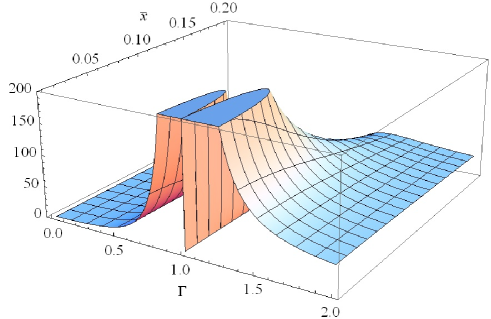
Figure 2: Fisher information $I(\hat{\rho}(\theta))$ as function of $\overline{x}\equiv\overline{x}_{\theta}$ and $\Gamma\equiv\Gamma_{\theta}$ for $\Gamma^{\prime}_{\theta}=\overline{p}_{\theta}=0$ in units of its value $2\pi$ for a coherent state ($\Gamma_{\theta}=1$) with the same $\overline{x}$. The plot is cut at $I(\hat{\rho}(\theta))=200.$

When expanding Eq. (18) close to this point ($\Gamma_{\theta}=1+\epsilon_{\theta}$ with $|\epsilon_{\theta}|\ll 1$), we find

$$I(\hat{\rho}^{(-)}(\theta))/(2\overline{x}_{\theta}^{\prime 2}) = 1+\left(1+\frac{2}{\overline{x}_{\theta}^{2}}\right)\epsilon_{\theta}+\left(\frac{1}{\overline{x}_{\theta}^{4}}+\frac{1}{\overline{x}_{\theta}^{2}}\right)\epsilon_{\theta}^{2}+{\cal O}(\epsilon_{\theta})^{3}\,.$$ (19)

Eq. (19) shows that indeed at $\epsilon_{\theta}=0$ we have the Fisher information of a coherent state, but at all finite values of $\epsilon_{\theta}$ one can reach arbitrarily large sensitivity in the limit of $\overline{x}_{\theta}\to 0$, as the lowest order in $\epsilon_{\theta}$ already diverges. Furthermore, the two limits $\overline{x}_{\theta}\to 0$ and $\Gamma_{\theta}\to 1$ do not commute. We just saw that taking $\Gamma_{\theta}\to 1$ first gives the finite coherent state result also in the limit $\overline{x}_{\theta}\to 0$ (i.e. the Fisher information of the vacuum state): $I(\hat{\rho}^{(-)}(\theta))=2\overline{x}_{\theta}^{\prime 2}$. However, the opposite order of limits gives, at $\overline{x}_{\theta}=0$, $I(\hat{\rho}^{(-)}(\theta))/\overline{x}_{\theta}^{\prime 2}=2\Gamma_{\theta}(3-2\Gamma_{\theta}+3\Gamma_{\theta}^{2})/(\Gamma_{\theta}-1)^{2}$, which diverges for $\Gamma_{\theta}\to 1$ as

$$I(\hat{\rho}^{(-)}(\theta))/\overline{x}_{\theta}^{\prime 2}=\frac{8}{(\Gamma_{\theta}-1)^{2}}+\frac{16}{\Gamma_{\theta}-1}+14+{\cal O}(\Gamma_{\theta}-1)\,.$$ (20)

Thus, the Fisher information is highly singular in the point $(\overline{x}_{\theta},\Gamma_{\theta})=(0,1)$, with a finite value on the line $\Gamma_{\theta}=1$ when approaching $\overline{x}_{\theta}\to 0$, but diverging on the line $\overline{x}_{\theta}=0$ when approaching $\Gamma_{\theta}\to 1$. Compared with the Fisher information for a Gaussian state, Eq. (12), that gives $2\Gamma_{\theta}\overline{x}_{\theta}^{\prime 2}$, we see that subtracting a photon can greatly enhance the Fisher information for the measurement of the same parameter.

One may wonder how this is compatible with the understanding that the quantum Cramér-Rao bound for the Gaussian state Pinel et al. (2012) gives the best possible sensitivity no matter what POVM measurement is performed on the state, and no matter how the data is analyzed. In particular one might argue that photon subtraction is achieved through interaction with another physical system and subsequent measurement, which one might think is describable by a set of POVMs. The resolution of the apparent paradox is through the observation that an essential step of photon subtraction is the selection of a sub-ensemble, heralded by the detection of a single photon as described above. However, that selection process makes the final state a non-linear function of the initial density matrix and therefore cannot be described by processing with a set of POVMs summing up to the identity matrix. Thus, the previously derived quantum Cramér-Rao bound Pinel et al. (2012) does not apply here, or in other words, photon subtraction (or addition) allows one to escape from the limitations on state processing on which the quantum Cramér-Rao bound is based.

We now study how useful the diverging Fisher information is. In particular, for $\overline{x}_{\theta}\to 0$ and in the limit of zero squeezing, the preparation of the state as described in Wenger et al. (2004); Kim (2008) by post-selection heralded on a single detected photon after passing through the beam splitter will fail almost always, such that the total measurement time including state preparation increases and the experimentally relevant sensitivity per square root of Hertz is reduced. Therefore, when taking the preparation time into account, the quantum Fisher information has to be appropriately rescaled, and the question is whether this removes its divergence.

A first observation is that the preparation scheme by Wenger et al. (2004); Kim (2008) is by no way unique. There might be more efficient preparation schemes that require a different renormalization of the Fisher information, or maybe none at all. Nevertheless, it is instructive to calculate the required renormalization for the particular preparation scheme in Wenger et al. (2004); Kim (2008). As we will show in the following, it turns out that the divergence of the Fisher information is completely removed. Therefore, when taking into account the increasing preparation time of the photon-subtracted state in the limit of an initial unsqueezed vacuum state, the experimentally relevant sensitivity per square root of Hertz cannot be increased to arbitrarily high levels, at least with this preparation scheme.

To demonstrate this, let us calculate the success probability for the preparation scheme, i.e. the probability to detect exactly one photon of the initial squeezed coherent state in the darker of the two output ports after it passes an almost transparent beam splitter. The two mode unitary transformation that describes the beam splitter is given by $\hat{U}_{BS}(\delta)=\exp(\delta(\hat{a}^{\dagger}\hat{b}-\hat{a}\hat{b}^{\dagger}))$, where $\hat{a},\hat{b}$ are annihilation operators respectively for the two modes, and $\delta$ is the mixing angle. Owing to the conservation of total photon-number $N$ by the beam splitter, it is convenient to represent $\hat{U}_{BS}$ in the dual-rail basis,

$$\langle k,N-k|\hat{U}_{BS}|m,N-m\rangle = \sqrt{\frac{k!(N-k)!}{m!(N-m)!}}\sum_{l={\rm Max}(m-k,0)}^{{\rm Min}(N-k,m)}{m\choose l}{N-m\choose N-k-l}$$ (21)

$$\times(-1)^{l}\left(\cos\delta\right)^{m+N-k-2l}\left(\sin\delta\right)^{k-m+2l}\,,$$

where the kets $|n,m\rangle$ denotes a product of photon number eigenstates with $n$ and $m$ photons, respectively, in the two modes Nielsen and Chuang (2010); Braun and Georgeot (2006).

Next we express the initial state $|\psi\rangle$ very generally in the photon number basis as $|\psi\rangle=\sum_{n=0}^{\infty}a_{n}|0,n\rangle$, with the first mode initially in the vacuum state. After the action of the beam splitter we have the final state $|\psi^{\prime}\rangle=\hat{U}_{BS}|\psi\rangle$. The probability to detect one photon in the first mode is then given by $P^{\mathrm{out}}_{1}=\sum_{n=0}^{\infty}|\langle 1,n|\psi^{\prime}\rangle|^{2}$. A few lines of calculation lead to

$$P^{\mathrm{out}}_{1}=\sum_{n=1}^{\infty}P_{n}n\left(\cos\delta\right)^{2(n-1)}\sin^{2}\delta\,,$$ (22)

where $P_{n}=|a_{n}|^{2}$ denotes the initial probabilities for $n$ photons in the input mode. For a squeezed coherent state, these probabilities are well known (see e.g. Eq. (3.5.16) in Scully and Zubairy (1997)). We adapt the notation of that reference in writing the squeezed coherent state as

$$|\alpha,\xi\rangle=\hat{S}(\xi)\hat{D}(\alpha)|0\rangle\,,$$ (23)

where $\hat{S}(\xi)$ and $\hat{D}(\alpha)$ are the usual squeeze and displacement operators, $\hat{S}(\xi)=\exp((\xi^{*}\hat{a}^{2}-\xi(\hat{a}^{\dagger})^{2})/2)$ with $\xi=re^{i\vartheta}$, $(r\geq 0$) and $\hat{D}(\alpha)=\exp(\alpha\hat{a}^{\dagger}-\alpha^{*}\hat{a})$. Then

$$P_{n}=\frac{(\tanh(r))^{n}}{2^{n}n!\cosh(r)}\exp\left(-|\alpha|^{2}+\frac{1}{2}\left(e^{-i\vartheta}\alpha^{2}+e^{i\vartheta}(\alpha^{*})^{2}\right)\tanh(r)\right)|H_{n}\left(\frac{\alpha e^{-i\vartheta/2}}{\sqrt{\sinh(2r)}}\right)|^{2}\,,$$ (24)

where $H_{n}(x)$ is the Hermite polynomial of order $n$.

A closed form of $P_{n}$ can be found in the case that interests us most, namely at $\alpha=0$, where we find

$$P^{\mathrm{out}}_{1}(\alpha=0,\delta)=\frac{\sin^{2}(2\delta){\rm sech}(r)\tanh^{2}(r)}{4(1-\cos^{4}\delta\tanh^{2}r)^{3/2}}\,.$$ (25)

The function is $\pi$-periodic in $\delta$ as to be expected. The squeezing angle $\vartheta$ has disappeared with the amplitude $\alpha\to 0$, as can be seen from Eq. (24). A plot of $P^{\mathrm{out}}_{1}$ as function of the remaining parameters $r$ and $\delta$ is shown in Fig. 3. We see that $P^{\mathrm{out}}_{1}$, as function of $\delta$, reaches a sharp maximum of about 0.2 if the squeezing is rather strong. The maximum moves with increasing squeezing closer and closer to $\delta=0$. For small squeezing $P^{\mathrm{out}}_{1}(\alpha=0,\delta)$ starts off quadratically, as is confirmed by expanding it about $r=0$,

$$P^{\mathrm{out}}_{1}(\alpha=0,\delta)=\frac{1}{4}\sin^{2}(2\delta)r^{2}+{\cal O}(r^{3})\mbox{ for }r\ll 1\,.$$ (26)

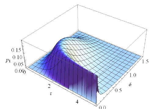
Figure 3: Success probability $p_{1}\equiv P_{1}^{\rm out}$) for preparation of the single photon subtracted squeezed coherent state for $\overline{x}_{\theta}=0$ as function of squeeze parameter $r$ and beam splitter mixing angle $\delta$.

Next we need to calculate the parameters $\Gamma_{\theta}$ and $x_{\theta}$ used so far for characterizing our Gaussian states. This is easily achieved with the results for the expectation values for $\hat{a}$, $\hat{a}^{2}$ and $\hat{a}^{\dagger}\hat{a}$ for squeezed coherent states found in Eq. (2.7.11) in Scully and Zubairy (1997). Inserting the result into the equation leading to Eq. (20), we find for the Fisher information, in the case of $\overline{p}_{\theta}=\overline{p}_{\theta}^{\prime}=\Gamma^{\prime}=0$,

$$I(\hat{\rho}^{(-)}(\theta))=\overline{x}_{\theta}^{\prime 2}\frac{4e^{4r}(-1+3\cosh(2r))}{(-1+e^{2r})^{2}}\,,$$ (27)

which for small $r$ diverges as $1/r^{2}$,

$$I(\hat{\rho}^{(-)}(\theta))=2\overline{x}_{\theta}^{\prime 2}\left(\frac{1}{r^{2}}+\frac{2}{r}+\frac{14}{3}+{\cal O}(r^{1})\right)$$ (28)

in agreement with Eq. (20). We are interested in the regime where $P^{\mathrm{out}}_{1}$ is small. This means that on the average one has to repeat the preparation attempt of the photon-subtracted state a number of times that scales as $1/P^{\mathrm{out}}_{1}$. Thus, in a given finite time, the number of measurements that can be done with a successfully prepared photon-subtracted state is proportional to $P^{\mathrm{out}}_{1}$. (In other words, if a single preparation takes a time $T$, the preparation rate is $P^{\mathrm{out}}_{1}/T$). Since the quantum Fisher information for a single shot measurement given by Eq. (9) is scaled by the number of measurements $Q$ in the QCRB, we have to rescale the QFI with a factor $P^{\mathrm{out}}_{1}$ in order to find the scaling of the effective quantum Fisher information that includes the preparation rate (giving a sensitivity with units $[\theta]\sqrt{\rm Hz}$). We see from Eq. (26) that the scaling of $P^{\mathrm{out}}_{1}$ with $r$ at small $r$ is quadratic, so it exactly cancels the $1/r^{2}$ divergence of the quantum Fisher information. The effective quantum Fisher information reads

$$I_{\mathrm{eff}}(\hat{\rho}^{(-)}(\theta))=\frac{1}{2}\overline{x}_{\theta}^{\prime 2}\sin^{2}(2\delta)+{\cal O}(r)\,.$$ (29)

Let us stress the parallel between this result and noiseless linear amplification, as first proposed by Xiang et al. in Xiang et al. (2010). In the same way as the noiseless amplification of an initial quantum state can occur non-deterministically by photon heralding, in the case we have studied it is possible to surpass the sensitivity of a Gaussian state in parameter estimation by photon subtraction, but only in a non deterministic way that is conditioned by the successful subtraction of one photon.

All of the above remains valid if the parameter dependence of the Gaussian state is carried by $\overline{p}_{\theta}$ instead of $\overline{x}_{\theta}$. The quantum Fisher information at $\alpha=0$ is then simply to be multiplied with $1/\Gamma_{\theta}^{2}$, which does not change the behavior at $\Gamma_{\theta}\to 1$.

Finally, if all parameter dependence is in $\Gamma_{\theta}$, i.e. if both shifts are independent of $\theta$, $\overline{x}_{\theta}^{\prime}=\overline{p}_{\theta}^{\prime}=\overline{p}=0$, we get a result that is asymptotically independent of $N$,

$$I(\hat{\rho}^{(-)}(\theta)) = \frac{\left(3+\Gamma_{\theta}\left(4\overline{x}^{4}\Gamma_{\theta}+4\overline{x}_{\theta}^{2}\left(3-2\Gamma_{\theta}+3\Gamma_{\theta}^{2}\right)+3\left(-4+6\Gamma_{\theta}-4\Gamma_{\theta}^{2}+\Gamma_{\theta}^{3}\right)\right)\right)\Gamma_{\theta}^{\prime 2}}{2\left(\Gamma_{\theta}+2\left(-1+\overline{x}_{\theta}^{2}\right)\Gamma_{\theta}^{2}+\Gamma_{\theta}^{3}\right)^{2}}$$ (30)

paralleling once more the behavior for Gaussian states Pinel et al. (2012). In the limit of initial vacuum, $\overline{x}_{\theta}=\overline{p}_{\theta}=0$, one finds $I(\hat{\rho}^{(-)}(\theta))=3\Gamma_{\theta}^{\prime 2}/(2\Gamma_{\theta}^{2})$, i.e. there is no divergence at $\Gamma_{\theta}\to 1$.

V QCR for Gaussian states with one photon added

V.1 General results

Photon addition leads to more complicated expressions, but the procedure for obtaining the QCR follows the same pattern as above. In order to simplify expressions a little we drop all subscripts $\theta$ in this section. We first find the Wigner function for the photon-added Gaussian state,

$$W(x,p)[\hat{\rho}^{+}] = \frac{e^{-\frac{(p-\overline{p})^{2}}{\Gamma}-(x-\overline{x})^{2}\Gamma}}{\pi\Gamma^{2}\left(2\left(3+\overline{p}^{2}+\overline{x}^{2}\right)+\Gamma^{-1}+\Gamma\right)}$$

$$\times \Big{(}2p^{2}+2\overline{p}^{2}+\left(-1+4p^{2}\right)\Gamma+2\left(1+p^{2}+x^{2}\right)\Gamma^{2}+\left(-1+4x^{2}-4x\overline{x}\right)\Gamma^{3}$$

$$+2(x-\overline{x})^{2}\Gamma^{4}-4p\overline{p}(1+\Gamma)\Big{)}\,.$$

Inserting this in Eq. (10), expanding in $x$ and $p$ up to the tenth order, integrating symbolically term by term, and adding up the terms from the expansion, we find the exact expression for the Fisher information, which can be found in the Appendix, in Eq. (VII).

V.2 Special and limiting cases

The expansion for large $\overline{x}$ leads to the exact same expression for the first two highest order terms in $N$ as for photon subtraction in Eq. (17). Thus, for large photon numbers, photon subtraction and addition are essentially equivalent concerning their usefulness for precision measurements, and, as mentioned above, the increase (or decrease, depending on the sign of the second term in Eq. (17)) is of relative order $1/N$ only.

If all the parameter dependence for a state centered at $\overline{p}=0$ is in the shift in $x$-direction, $\Gamma^{\prime}=0=\overline{p}=\overline{p}^{\prime}=0$, we find

$$I(\hat{\rho}^{(+)}(\theta)) = \frac{2}{(1+2(3+\overline{x}^{2})\Gamma+\Gamma^{2})^{4}}$$

$$\times \Big{\{}\Gamma(3+4(13+3\overline{x}^{2})\Gamma+4(83+8\overline{x}^{2}+4\overline{x}^{4})\Gamma^{2}+4(239+135\overline{x}^{2}+52\overline{x}^{4}+4\overline{x}^{6})\Gamma^{3}$$

$$+2(593+784\overline{x}^{2}+432\overline{x}^{4}+96\overline{x}^{6}+8\overline{x}^{8})\Gamma^{4}+4(91+177\overline{x}^{2}+84\overline{x}^{4}+12\overline{x}^{6})\Gamma^{5}$$

$$+4(35+48\overline{x}^{2}+12\overline{x}^{4})\Gamma^{6}+4(9+5\Gamma^{2})\Gamma^{7}+3\Gamma^{8})\overline{x}^{\prime 2}\Big{\}}\,.$$

We see once more the leading behavior $\propto N$ due to the terms $\overline{x}^{8}\overline{x}^{\prime 2}/\overline{x}^{8}$. However, contrary to photon subtraction, no divergence is observed for $N\ll 1$, regardless of the squeezing, as the possibly vanishing term $(-1+\overline{x}^{2})$ in the denominator for the photon-subtracted case is now replaced by $3+\overline{x}^{2}>0$.

Finally, if both shifts are independent of $\theta$, $\overline{x}^{\prime}=\overline{p}^{\prime}=\overline{p}=0$, we have

$$I(\hat{\rho}^{(+)}(\theta)) = \frac{1}{2\Gamma^{2}(1+2(3+\overline{x}^{2})\Gamma+\Gamma^{2})^{4}}$$

$$\times \Big{\{}(3+24(2+\overline{x}^{2})\Gamma+4(105+88\overline{x}^{2}+16\overline{x}^{4})\Gamma^{2}+8(114+149\overline{x}^{2}+60\overline{x}^{4}+8\overline{x}^{6})\Gamma^{3}$$

$$+2(665+992\overline{x}^{2}+480\overline{x}^{4}+96\overline{x}^{6}+8\overline{x}^{8})\Gamma^{4}+8(114+149\overline{x}^{2}+60\overline{x}^{4}+8\overline{x}^{6})\Gamma^{5}$$

$$+4(105+88\overline{x}^{2}+16\overline{x}^{4})\Gamma^{6}+24(2+\overline{x}^{2})\Gamma^{7}+3\Gamma^{8})(\Gamma^{\prime})^{2}\Big{\}}\,.$$

In the limit of initial vacuum (i.e. in addition $\overline{x}\to 0$), the expression converges to

$$I(\hat{\rho}^{(+)}(\theta)) = \frac{\left(3+48\Gamma+420\Gamma^{2}+912\Gamma^{3}+1330\Gamma^{4}+912\Gamma^{5}+420\Gamma^{6}+48\Gamma^{7}+3\Gamma^{8}\right)(\Gamma^{\prime})^{2}}{2\Gamma^{2}\left(1+6\Gamma+\Gamma^{2}\right)^{4}}\,.$$ (34)

For large $\Gamma$ this expression decays just as in the photon subtracted state, i.e. as $3(\Gamma^{\prime})^{2}/(2\Gamma^{2})$.

VI Conclusions

For large number of photon $N$, subtraction (or addition) of a single photon from (or to) a pure Gaussian state does not substantially alter the scaling with $N$ of the sensitivity with which one can estimate a parameter $\theta$ coded in the initial Gaussian state. The corrections to the quantum Fisher information are only of relative order $1/N$. For small $N$, photon subtraction can increase the sensitivity attainable with squeezed states, in particular for almost vanishing squeezing parameter $r$ and $N\ll 1$. The quantum Fisher information diverges as $1/r^{2}$ in that limit, reflecting the extremely non-classical behavior of such a state. However, in the standard preparation scheme, based on the passage of a squeezed coherent state through a beam splitter that is almost transparent for the state, and heralding an output based on the detection of a single photon in the almost dark output port Wenger et al. (2004); Kim (2008), the success probability of the preparation decays proportionally to $r^{2}$ with the squeezing parameter. The rescaled quantum Fisher information for the experimentally relevant sensitivity in a fixed bandwidth that takes into account the preparation time of the state is given by the product of the success probability and the single shot quantum Fisher information. This leads to an exact cancellation of the divergence of the Fisher information. It remains to be seen whether there are deterministic preparation schemes or experimental niches where such states that use essentially no light at all can compete with the standard approach of very large photon numbers.

Acknowledgments: We thank Claude Fabre for useful discussions. O.P. acknowledges support by the Australian Research Council Centre of Excellence for Quantum Computation and Communication Technology, project number CE110001027. This work is supported by the European Research Council starting grant Frecquam.

VII Appendix

Here we report the exact Fisher information for the photon-added state. For improving the readability, we skip all the subscripts $\theta$, but it is understood that $\overline{x}$, $\overline{p}$, and $\Gamma$ depend on $\theta$, and ^′ denotes $d/d\theta$.

$$I(\hat{\rho}^{(+)}(\theta)) = \frac{1}{2\Gamma^{2}(1+2(3+\overline{p}^{2}+\overline{x}^{2})\Gamma+\Gamma^{2})^{4}}$$

$$\times \Big{\{}16(9+3\overline{p}^{2}+5\overline{x}^{2})\Gamma^{10}(\overline{x}^{\prime})^{2}+12\Gamma^{11}(\overline{x}^{\prime})^{2}+4\Gamma^{9}(3(\overline{p}^{\prime})^{2}+4(35+4\overline{p}^{4}+12\overline{x}^{2}(4+\overline{x}^{2})$$

$$+8\overline{p}^{2}(3+2\overline{x}^{2}))(\overline{x}^{\prime})^{2})+3(\Gamma^{\prime})^{2}+\Gamma^{8}(16(13+3\overline{p}^{2}+5\overline{x}^{2})(\overline{p}^{\prime})^{2}+16(91+103\overline{p}^{2}$$

$$+36\overline{p}^{4}+4\overline{p}^{6}+(177+20\overline{p}^{2}(6+\overline{p}^{2}))\overline{x}^{2}+28(3+\overline{p}^{2})\overline{x}^{4}+12\overline{x}^{6})(\overline{x}^{\prime})^{2}-32\overline{x}\overline{x}^{\prime}\Gamma^{\prime}$$

$$+3(\Gamma^{\prime})^{2})+12\Gamma((\overline{p}^{\prime})^{2}+2(2+\overline{p}^{2}+\overline{x}^{2})(\Gamma^{\prime})^{2})+4\Gamma^{2}(4(9+5\overline{p}^{2}+3\overline{x}^{2})(\overline{p}^{\prime})^{2}+8\overline{p}\overline{p}^{\prime}\Gamma^{\prime}$$

$$+(7+4\overline{p}^{2}+4\overline{x}^{2})(15+4\overline{p}^{2}+4\overline{x}^{2})(\Gamma^{\prime})^{2})+2\Gamma^{4}(8(91+12\overline{p}^{6}+103\overline{x}^{2}+28\overline{p}^{4}(3+\overline{x}^{2})$$

$$+4\overline{x}^{4}(9+\overline{x}^{2})+\overline{p}^{2}(177+20\overline{x}^{2}(6+\overline{x}^{2})))(\overline{p}^{\prime})^{2}+8(13+5\overline{p}^{2}+3\overline{x}^{2})(\overline{x}^{\prime})^{2}$$

$$+16(2\overline{p}(33+20\overline{x}^{2}+4(\overline{p}^{4}+\overline{x}^{4}+\overline{p}^{2}(5+2\overline{x}^{2})))\overline{p}^{\prime}$$

$$-\overline{x}(45+4\overline{p}^{4}+8\overline{p}^{2}(4+\overline{x}^{2})+4\overline{x}^{2}(8+\overline{x}^{2}))\overline{x}^{\prime})\Gamma^{\prime}+(665+992\overline{x}^{2}+8(\overline{p}^{8}+4\overline{p}^{6}(3+\overline{x}^{2})$$

$$+6\overline{p}^{4}(10+6\overline{x}^{2}+\overline{x}^{4})+\overline{x}^{4}(60+12\overline{x}^{2}+\overline{x}^{4})+4\overline{p}^{2}(31+30\overline{x}^{2}+9\overline{x}^{4}+\overline{x}^{6})))(\Gamma^{\prime})^{2})$$

$$+8\Gamma^{7}(2(83+8\overline{p}^{2}+4\overline{p}^{4}+16(4+\overline{p}^{2})\overline{x}^{2}+12\overline{x}^{4})(\overline{p}^{\prime})^{2}$$

$$+(593+784\overline{x}^{2}+8(\overline{p}^{8}+4\overline{p}^{6}(3+\overline{x}^{2})+6\overline{p}^{4}(3+\overline{x}^{2})^{2}+\overline{x}^{4}(54+12\overline{x}^{2}+\overline{x}^{4})$$

$$+2\overline{p}^{2}(53+2\overline{x}^{2}(27+9\overline{x}^{2}+\overline{x}^{4}))))(\overline{x}^{\prime})^{2}$$

$$-4\overline{x}(19+5\overline{p}^{2}+5\overline{x}^{2})\overline{x}^{\prime}\Gamma^{\prime}+3(2+\overline{p}^{2}+\overline{x}^{2})(\Gamma^{\prime})^{2}+4\overline{p}\overline{p}^{\prime}(-32\overline{x}\overline{x}^{\prime}+(-1+\overline{p}^{2}+\overline{x}^{2})\Gamma^{\prime}))$$

$$+8\Gamma^{5}((593+848\overline{x}^{2}+8(\overline{p}^{8}+4\overline{p}^{6}(3+\overline{x}^{2})+6\overline{p}^{4}(3+\overline{x}^{2})^{2}+\overline{x}^{4}(54+12\overline{x}^{2}+\overline{x}^{4})$$

$$+2\overline{p}^{2}(49+2\overline{x}^{2}(27+9\overline{x}^{2}+\overline{x}^{4}))))(\overline{p}^{\prime})^{2}+2(83+8\overline{x}^{2}+4(3\overline{p}^{4}+\overline{x}^{4}+4\overline{p}^{2}(4+\overline{x}^{2})))(\overline{x}^{\prime})^{2}$$

$$-8\overline{x}(3+\overline{p}^{2}+\overline{x}^{2})(21+2\overline{p}^{4}+4\overline{p}^{2}(3+\overline{x}^{2})+2\overline{x}^{2}(6+\overline{x}^{2}))\overline{x}^{\prime}\Gamma^{\prime}$$

$$+(114+8\overline{p}^{6}+149\overline{x}^{2}+60\overline{x}^{4}+8\overline{x}^{6}+12\overline{p}^{4}(5+2\overline{x}^{2})+\overline{p}^{2}(149+24\overline{x}^{2}(5+\overline{x}^{2})))(\Gamma^{\prime})^{2}$$

$$+8\overline{p}\overline{p}^{\prime}(-16\overline{x}\overline{x}^{\prime}+(3+\overline{p}^{2}+\overline{x}^{2})(21+2\overline{p}^{4}+4\overline{p}^{2}(3+\overline{x}^{2})+2\overline{x}^{2}(6+\overline{x}^{2}))\Gamma^{\prime}))$$

$$+4\Gamma^{6}(4(239+135\overline{p}^{2}+52\overline{p}^{4}+4\overline{p}^{6}+(273+152\overline{p}^{2}+20\overline{p}^{4})\overline{x}^{2}+4(25+7\overline{p}^{2})\overline{x}^{4}+12\overline{x}^{6})(\overline{p}^{\prime})^{2}$$

$$+4(239+12\overline{p}^{6}+135\overline{x}^{2}+52\overline{x}^{4}+4\overline{x}^{6}+4\overline{p}^{4}(25+7\overline{x}^{2})+\overline{p}^{2}(273+152\overline{x}^{2}+20\overline{x}^{4}))(\overline{x}^{\prime})^{2}$$

$$-16\overline{x}(33+20\overline{x}^{2}+4(\overline{p}^{4}+\overline{x}^{4}+\overline{p}^{2}(5+2\overline{x}^{2})))\overline{x}^{\prime}\Gamma^{\prime}$$

$$+(7+4\overline{p}^{2}+4\overline{x}^{2})(15+4\overline{p}^{2}+4\overline{x}^{2})(\Gamma^{\prime})^{2}+8\overline{p}\overline{p}^{\prime}(-64\overline{x}\overline{x}^{\prime}+(45+4\overline{p}^{4}+8\overline{p}^{2}(4+\overline{x}^{2})$$

$$+4\overline{x}^{2}(8+\overline{x}^{2}))\Gamma^{\prime}))+4\Gamma^{3}(4(35+12\overline{p}^{4}+16\overline{p}^{2}(3+\overline{x}^{2})+4\overline{x}^{2}(6+\overline{x}^{2}))(\overline{p}^{\prime})^{2}+3(\overline{x}^{\prime})^{2}$$

$$+8\overline{p}(19+5\overline{p}^{2}+5\overline{x}^{2})\overline{p}^{\prime}\Gamma^{\prime}+2\Gamma^{\prime}(-4\overline{x}(-1+\overline{p}^{2}+\overline{x}^{2})\overline{x}^{\prime}$$

$$+114\Gamma^{\prime}+(\overline{p}^{2}+\overline{x}^{2})(149+8\overline{p}^{4}+60\overline{x}^{2}+8\overline{x}^{4}+4\overline{p}^{2}(15+4\overline{x}^{2}))\Gamma^{\prime}))\Big{\}}\,.$$

References

- Kim et al. (2005) M. Kim, E. Park, P. Knight, and H. Jeong, Physical Review A 71, 043805 (2005).
- Mandel (1986) L. Mandel, Physica scripta 1986, 34 (1986).
- Hudson (1974) R. Hudson, Reports on Mathematical Physics 6, 249 (1974).
- Soto and Claverie (1983) F. Soto and P. Claverie, Journal of Mathematical Physics 24, 97 (1983).
- Mandilara et al. (2009) A. Mandilara, E. Karpov, and N. J. Cerf, Physical Review A 79, 062302 (2009).
- Caves (1981) C. M. Caves, Phys. Rev. D 23, 1693 (1981).
- Keller et al. (2008) G. Keller, V. D’Auria, N. Treps, T. Coudreau, J. Laurat, and C. Fabre, Optics Express 16, 9351 (2008).
- Abadie et al. (2011) J. Abadie, B. Abbott, R. Abbott, T. Abbott, M. Abernathy, C. Adams, R. Adhikari, C. Affeldt, B. Allen, G. Allen, et al., Nature Physics 7, 962 (2011).
- Braunstein and van Loock (2005) S. L. Braunstein and P. van Loock, Rev. Mod. Phys. 77, 513 (2005).
- Mari and Eisert (2012) A. Mari and J. Eisert, Physical review letters 109, 230503 (2012).
- Dakna et al. (1997) M. Dakna, T. Anhut, T. Opatrnỳ, L. Knöll, and D.-G. Welsch, Physical Review A 55, 3184 (1997).
- Wenger et al. (2004) J. Wenger, R. Tualle-Brouri, and P. Grangier, Physical review letters 92, 153601 (2004).
- Kim (2008) M. Kim, arXiv preprint arXiv:0807.4708 (2008).
- Neergaard-Nielsen et al. (2011) J. S. Neergaard-Nielsen, M. Takeuchi, K. Wakui, H. Takahashi, K. Hayasaka, M. Takeoka, M. Sasaki, A. Furusawa, B. M. Nielsen, E. S. Polzik, et al., Progress in Informatics 8, 5 (2011).
- Ourjoumtsev et al. (2007) A. Ourjoumtsev, A. Dantan, R. Tualle-Brouri, and P. Grangier, Physical Review Letters 98, 030502 (2007).
- Lee et al. (2011) S.-Y. Lee, S.-W. Ji, H.-J. Kim, and H. Nha, Physical Review A 84, 012302 (2011).
- Navarrete-Benlloch et al. (2012) C. Navarrete-Benlloch, R. García-Patrón, J. H. Shapiro, and N. J. Cerf, Physical Review A 86, 012328 (2012).
- Ferreyrol et al. (2010) F. Ferreyrol, M. Barbieri, R. Blandino, S. Fossier, R. Tualle-Brouri, and P. Grangier, Physical review letters 104, 123603 (2010).
- Xiang et al. (2010) G.-Y. Xiang, T. Ralph, A. Lund, N. Walk, and G. J. Pryde, Nature Photonics 4, 316 (2010).
- Bimbard et al. (2010) E. Bimbard, N. Jain, A. MacRae, and A. Lvovsky, Nature Photonics 4, 243 (2010).
- Zavatta et al. (2009) A. Zavatta, V. Parigi, M. Kim, H. Jeong, and M. Bellini, Physical review letters 103, 140406 (2009).
- Takahashi et al. (2008) H. Takahashi, K. Wakui, S. Suzuki, M. Takeoka, K. Hayasaka, A. Furusawa, and M. Sasaki, Physical review letters 101, 233605 (2008).
- Gerrits et al. (2010) T. Gerrits, S. Glancy, T. S. Clement, B. Calkins, A. E. Lita, A. J. Miller, A. L. Migdall, S. W. Nam, R. P. Mirin, and E. Knill, Physical Review A 82, 031802 (2010).
- Nha and Carmichael (2004) H. Nha and H. Carmichael, Physical Review Letters 93, 020401 (2004).
- García-Patrón et al. (2004) R. García-Patrón, J. Fiurášek, N. Cerf, J. Wenger, R. Tualle-Brouri, and P. Grangier, Physical review letters 93, 130409 (2004).
- Parigi et al. (2007) V. Parigi, A. Zavatta, M. Kim, and M. Bellini, Science 317, 1890 (2007).
- Bartley et al. (2013) T. J. Bartley, P. J. Crowley, A. Datta, J. Nunn, L. Zhang, and I. Walmsley, Physical Review A 87, 022313 (2013).
- Lee et al. (2013) S.-Y. Lee, S.-W. Ji, and C.-W. Lee, Phys. Rev. A 87, 052321 (2013).
- Kim et al. (2012) H.-J. Kim, S.-Y. Lee, S.-W. Ji, and H. Nha, Phys. Rev. A 85, 013839 (2012).
- Pinel et al. (2012) O. Pinel, J. Fade, D. Braun, P. Jian, N. Treps, and C. Fabre, Physical Review A 85, 010101 (2012).
- Pinel et al. (2013) O. Pinel, P. Jian, N. Treps, C. Fabre, and D. Braun, Phys. Rev. A 88, 040102 (2013).
- Monras (2013) A. Monras, arXiv preprint arXiv:1303.3682 (2013).
- Giovannetti et al. (2004) V. Giovannetti, S. Lloyd, and L. Maccone, Science 306, 1330 (2004).
- Wolfgramm et al. (2012) F. Wolfgramm, C. Vitelli, F. A. Beduini, N. Godbout, and M. W. Mitchell, Nature Photonics 7, 28 (2012).
- Gardiner and Zoller (2004) C. Gardiner and P. Zoller, Quantum noise: a handbook of Markovian and non-Markovian quantum stochastic methods with applications to quantum optics, vol. 56 (Springer, 2004).
- Schleich (2011) W. P. Schleich, Quantum optics in phase space (Wiley. com, 2011).
- Rao (1945) C. R. Rao, Bulletin of the Calcutta Mathematical Society 37, 81 (1945).
- Cramér (1999) H. Cramér, Mathematical Methods of Statistics (PMS-9), vol. 9 (Princeton university press, 1999).
- Braunstein and Caves (1994) S. L. Braunstein and C. M. Caves, Physical Review Letters 72, 3439 (1994).
- Nielsen and Chuang (2010) M. A. Nielsen and I. L. Chuang, Quantum computation and quantum information (Cambridge university press, 2010).
- Braun and Georgeot (2006) D. Braun and B. Georgeot, Physical Review A 73, 022314 (2006).
- Scully and Zubairy (1997) M. O. Scully and M. S. Zubairy, Quantum Optics (Cambridge University Press, 1997).