A Well-Balanced Scheme For Two-Fluid Flows In Variable Cross-Section ducts

Abstract

We propose a finite volume scheme for computing two-fluid flows in variable cross-section ducts. Our scheme satisfies a well-balanced property. It is based on the VFRoe approach. The VFRoe variables are the Riemann invariants of the stationnary wave and the cross-section. In order to avoid spurious pressure oscillations, the well-balanced approach is coupled with an ALE (Arbitrary Lagrangian Eulerian) technique at the interface and a random sampling remap.

Introduction

Classical finite volume solvers generally have a bad precision for solving two-fluid interfaces or flows in varying cross-section ducts. Several cures have been developed for improving the precision.

• For cross-section ducts, the well-balanced approach of Greenberg and Leroux [4] (see also [7] and [5]) is an efficient tool to improve the precision.

• For two-fluid flows the pressure oscillations phenomenon (see [6] and [2] for instance) can be cured by a recent tool developed in [3] and [1]. It is based on an ALE (Arbitrary Lagrangian Eulerian) scheme followed by a random sampling projection step.

In this paper, we show that is is possible to mix the two approaches in order to design an efficient scheme for computing two-fluid flows in variable cross-section ducts.

1 A well-balanced two-fluid ALE solver

1.1 Model

We consider the flow of a mixture of two compressible fluids (a gas (1) and a liquid (2), for instance) in a cross-section duct. The time variable is noted $t$ and the space variable along the duct is $x$. We denote by $A(x)$ the cross-section at position $x$. The unknowns are the density $\rho(x,t),$ the velocity $u(x,t)$, the internal energy $e(x,t)$ and the fraction of gas $\varphi(x,t)$. Following Greenberg and Leroux [4] it is now classical to consider the cross-section $A$ as an artificial unknown. The equations are the Euler equations in a duct, which read

$$\partial_{t}(A\rho)+\partial_{x}(A\rho u) = 0,$$ (1)

$$\partial_{t}(A\rho u)+\partial_{x}(A(\rho u^{2}+p)) = p\partial_{x}A,$$ (2)

$$\partial_{t}(A\rho E)+\partial_{x}(A(\rho E+p)u) = 0,$$ (3)

$$\partial_{t}(A\rho\varphi)+\partial_{x}(A\rho\varphi u) = 0,$$ (4)

$$\partial_{t}A = 0,$$ (5)

with

$$p=p(\rho,e,\varphi),$$ (6)

$$E=e+\frac{u^{2}}{2}.$$ (7)

Without loss of generality, in this paper we consider a stiffened gas pressure law (see [8] and included references)

$$p(\rho,e,\varphi)=(\gamma(\varphi)-1)\rho e-\gamma(\varphi)\pi(\varphi).$$ (8)

The mixture pressure law parameters $\gamma(\varphi)$ and $\pi(\varphi)$ are obtained from the pure fluid parameters $\gamma_{i}>1,\pi_{i}$, $i=1,2$ thanks to the following interpolation, which is justified in [2]

$$\frac{1}{\gamma(\varphi)-1} = \varphi\frac{1}{\gamma_{1}-1}+(1-\varphi)\frac{1}{\gamma_{2}-1},$$ (9)

$$\frac{\gamma(\varphi)\pi(\varphi)}{\gamma(\varphi)-1} =\varphi \frac{\gamma_{1}\pi_{1}}{\gamma_{1}-1}+(1-\varphi)\frac{\gamma_{2}\pi_{2}}{\gamma_{2}-1}.$$ (10)

We define the vector of conservative variables

$$W=(A\rho,A\rho u,A\rho E,A\rho\varphi,A)^{T}.$$ (11)

The conservative flux is

$$F(W)=(A\rho u,A(\rho u^{2}+p),A(\rho E+p)u,A\rho\varphi u,0)^{T},$$ (12)

and the non-conservative source term is

$$S=(0,p\partial_{x}A,0,0,0),$$ (13)

such that the system (1)-(5) becomes

$$\partial_{t}W+\partial_{x}F(W)=S(W).$$ (14)

We define the vector of primitive variables

$$Y=(\rho,u,p,\varphi,A)^{T}.$$ (15)

We define also the following quantities

$$Q = \text{mass flow rate}=\rho Au,$$ (16)

$$s = \text{entropy}=(p+\pi(\varphi))\rho^{-\gamma(\varphi)},$$ (17)

$$h = \text{enthalpy}=e+\frac{p}{\rho},$$ (18)

$$H = \text{total enthalpy}=h+\frac{u^{2}}{2}.$$ (19)

The entropy is solution of the partial differential equation

$$Tds=de-\frac{p}{\rho^{2}}d\rho+\lambda d\varphi.$$ (20)

It is useful to express also the pressure $p$ and the enthalpy $h$ as functions of $(\rho,s,\varphi)$

$$p=p(\rho,s,\varphi),\quad h=h(\rho,s,\varphi).$$ (21)

Then in these variables the sound speed $c$ satisfies

$$c^{2}=p_{\rho}=\rho h_{\rho}.$$ (22)

The jacobian matrix $F^{\prime}(W)$ in system (14) admits real eigenvalues

$$\lambda_{0}=0,\quad\lambda_{1}=u-c,\quad\lambda_{2}=\lambda_{3}=u,\quad\lambda_{4}=u+c.$$ (23)

However, the system may be resonant (when $\lambda_{0}=\lambda_{1}$ or $\lambda_{0}=\lambda_{4}$.) The quantities $\varphi$, $s$, $Q$ and $H$ are independant Riemann invariants of the stationnary wave $\lambda_{0}$. In the sequel, the vector of “stationary” variables $Z$ will play a particular role

$$Z=(A,\varphi,s,Q,H)^{T}.$$ (24)

1.2 VFRoe ALE numerical flux

We recall now the principles of the VFRoe solver. We first consider a arbitrary change of variables $U=U(W)$. In practice, we will take the set of primitive variables $U=Y$ (15) or the set of stationnary variables $U=Z$ (24). The vector $U$ satisfies a non-conservative set of equations

$$\partial_{t}U+C(U)\partial_{x}U=0.$$ (25)

The system (1)-(5) is approximated by a finite volume scheme with cells $]x_{i-1/2},x_{i+1/2}[$, $i\in\mathbb{Z}$. We denote by $\tau$ the time step and by $\Delta x_{i}=x_{i+1/2}-x_{i-1/2}$ the size of cell $i$. We denote by $W_{i}^{n}$ the conservative variables in cell $i$ at time step $n$. The cross-section $A$ is approximated by a piecewise constant function, $A=A_{i}$ in cell $i$.

We consider first a very general scheme where the boundary of the cell $x_{i+1/2}$ moves at the velocity $v_{i+1/2}^{n}$ between time steps $n$ and $n+1$, thus we have

$$x_{i+1/2}^{n+1}=x_{i+1/2}^{n}+\tau v_{i+1/2}^{n}.$$ (26)

In a VFRoe-type scheme, we have to define linearized Riemann problems at interface $i+1/2$ between the state $W_{L}=W_{i}^{n}$ and $W_{R}=W_{i+1}^{n}$, we introduce

$$\overline{U}=\frac{1}{2}(U_{L}+U_{R}).$$ (27)

In this way, it is possibe to define

$$\overline{W}=W(\overline{U}),\quad\overline{C}=C(\overline{U}).$$ (28)

We then consider the linearized Riemann problem

$$\partial_{t}U+\overline{C}\partial_{x}U = 0,$$ (29)

$$U(x,\text{0)} = \left\{\begin{array}[]{c}U_{L}\text{ if }x<0,\\ U_{R}\text{ if }x>0.\end{array}\right.$$ (32)

We denote its solution by

$$U(U_{L},U_{R},\frac{x}{t})=U(x,t).$$ (33)

Because of the stationary wave, $U(U_{L},U_{R},\frac{x}{t})$ is generally discontinuous at $x/t=0.$ We are then able to define a discontinuous Arbitrary Lagrangian Eulerian (ALE) numerical flux

$$F(W_{L},W_{R},v^{\pm}):=F(W(U(U_{L},U_{R},v^{\pm})))-vW(U(U_{L},U_{R},v^{\pm})).$$ (34)

The sizes of the cells evolve as

$$\Delta x_{i}^{n+1}=\Delta x_{i}^{n}+\tau(v_{i+1/2}^{n}-v_{i-1/2}^{n}).$$ (35)

If $v_{i+1/2}^{n}\leq 0$ and $v_{i-1/2}^{n}\geq 0$, the ALE scheme is

$$\Delta x_{i}^{n+1}W_{i}^{n+1,-}-\Delta x_{i}^{n}W_{i}^{n}+$$

$$\tau\left(F(W_{i}^{n},W_{i+1}^{n},v_{i+1/2}^{n,-})-F(W_{i-1}^{n},W_{i}^{n},v_{i-1/2}^{n,+})\right) = 0.$$ (36)

If $v_{i+1/2}^{n}>0$ then we have to add the following term to the left of the previous equation

$$\tau\left(F(W_{i}^{n},W_{i+1}^{n},0^{-})-F(W_{i}^{n},W_{i+1}^{n},0^{+})\right).$$ (37)

If $v_{i-1/2}^{n}<0$ then we have to add also the following term

$$\tau\left(F(W_{i-1}^{n},W_{i}^{n},0^{-})-F(W_{i-1}^{n},W_{i}^{n},0^{+})\right).$$ (38)

1.3 ALE velocity

We have now to detail the choice of the variable $U$ and the velocity $v$ according to the data $W_{L}$ and $W_{R}$. The idea is to use the classical well-balanced scheme everywhere but at the interface between the two fluids, where we use the Lagrange flux. When our initial data satisfy $\varphi\in\{0,1\}$, the algorithm reads

• If we are not at the interface, i.e. if $\varphi_{L}=\varphi_{R}$, we take $U=Z$ and $v=0$. This choice corresponds to the VFRoe well-balanced scheme described in [5].

• If we are at the interface, i.e. if $\varphi_{L}\neq\varphi_{R}$ then we choose $U=Y$. This choice ensures that the linearized Riemann solver presents no jump of pressure and velocity at the contact discontinuity. We thus denote by $u^{*}(W_{L},W_{R})$ and $p^{*}(W_{L},W_{R})$ the velocity and the pressure at the contact. We take $v=u^{*}(W_{L},W_{R})$, $A^{*}=A_{L}$ if $v<0$ and $A^{*}=A_{R}$ if $v>0$. The lagrangian numerical flux then takes the form

  $$F(W_{L},W_{R},v^{\pm})=(0,A^{*}p^{*},A^{*}u^{*}p^{*},0,-A^{*}u^{*})^{T}.$$ (39)

1.4 Glimm remap

We go back to the original Euler grid by the Glimm procedure.

We construct a sequence of pseudo-random numbers $\omega_{n}\in[0,1[.$ In practice, we consider the $(5,3)$ van der Corput sequence [1]. According to this number we take

$$W_{i}^{n+1}=W_{i-1}^{n+1,-}\text{ if }\omega_{n}<\frac{\tau_{n}}{\Delta x_{i}}\max(v_{i-1/2}^{n},0),$$ (40)

$$W_{i}^{n+1}=W_{i+1}^{n+1,-}\text{ if }\omega_{n}>1+\frac{\tau_{n}}{\Delta x_{i}}\min(v_{i+1/2}^{n},0),$$ (41)

$$W_{i}^{n}=W_{i}^{n+1,-}\text{ if }\frac{\tau_{n}}{\Delta x_{i}}\max(v_{i-1/2}^{n},0)\leq\omega_{n}\leq 1+\frac{\tau_{n}}{\Delta x_{i}}\min(v_{i+1/2}^{n},0).$$ (42)

1.5 Properties of the scheme

The constructed scheme has many interesting properties:

• it is well-balanced in the sense that it preserves exactly all stationary states (i.e. initial data for which the quantities $\varphi,s,Q,H$ are constant);

• for constant cross-section ducts, it computes exactly the contact discontinuities, with no smearing of the density and the mass fraction;

• if at the initial time the mass fraction is in $\{0,1\}$, then this property is exactly preserved at any time.

For detailed proofs, we refer to [5] and [1]. Some other subtleties are given in the same references. For instance, the change of variables $Z=Z(W)$ is not always invertible. This implies to define a special procedure for constructing completely rigorously the well-balanced VFRoe solver.

2 Numerical results

In order to test our algorithm, we consider a Riemann problem for which we know the exact solution. The initial data are discontinuous at $x=1$. The data of the problem are given in Table 1

quantity	Left	Right
$\rho$	2	3.230672602
$u$	0.5	-0.4442565900
$p$	1	12
$\varphi$	1	0
$A$	1.5	1

Table 1: Numerical results. Data of the Riemann problem

The pressure law parameters are $\gamma_{1}=1.4$, $\pi_{1}=0$, $\gamma_{2}=1.6$ and $\pi_{2}=2.$ We compute the solution on the domain $[0.4;1.6]$ with approximately $2000$ cells. The final time is $T=0.2$ and the CFL number is $0.6$. The density, the velocity and the pressure are represented on Figures 1, 2 and 3. We observe an excellent agreement between the exact and the approximate solution. The mass fraction is not represented: it is not smeared at all and perfectly matches the exact solution.

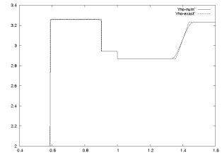
Figure 1: Two-fluid, discontinuous cross-section Riemann problem. Density plot. Comparison of the exact solution (dotted line) and the approximate one (continuous line)

Figure 2: Two-fluid, discontinuous cross-section Riemann problem. Pressure plot. Comparison of the exact solution (dotted line) and the approximate one (continuous line)

Figure 3: Two-fluid, discontinuous cross-section Riemann problem. Velocity plot. Comparison of the exact solution (dotted line) and the approximate one (continuous line)

3 Conclusion

We have constructed and validated a new scheme for computing two-fluid flows in variable cross-section ducts. Our scheme relies on two ingredients:

• a well-balanced approach for dealing with the varying cross-section;

• a Lagrange plus remap technique in order to avoid pressure oscillations at the interface. The random sampling remap ensures that the interface is not diffused at all.

On preliminary test cases, our approach gives very satisfactory results. We intend to apply it to the computation of the oscillations of cavitation bubbles. More results will be presented at the conference.

The authors wish to thank Jean-Marc Hérard for many fruitful discussions.

References

• [1] M. Bachmann, P. Helluy, H. Mathis, S. Mueller. Random sampling remap for compressible two-phase flows. Preprint HAL http://hal.archives-ouvertes.fr/hal-00546919/fr/
• [2] T. Barberon, P. Helluy, S. Rouy. Practical computation of axisymmetrical multifluid flows. Int. J. Finite Vol. 1 (2004), no. 1, 34 pp. http://ijfv.org
• [3] C. Chalons, F. Coquel. Computing material fronts with a Lagrange-Projection approach. HYP2010 Proc. http://hal.archives-ouvertes.fr/hal-00548938/fr/
• [4] J.-M. Greenberg, A.Y., Leroux. A well balanced scheme for the numerical processing of source terms in hyperbolic equations”, SIAM J. Num. Anal., vol. 33 (1), pp. 1–16, 1996.
• [5] P. Helluy, J.-M. HΓ©rard, H. Mathis. A Well- Balanced Approximate Riemann Solver for Variable Cross- Section Compressible Flows. AIAA-2009-3540. 19th AIAA Computational Fluid Dynamics. June 2009.
• [6] S. Karni. Multicomponent flow calculations by a consistent primitive algorithm. J. Comput. Phys. 112 (1994), no. 1, 31–43
• [7] D. Kroner, M.-D. Thanh. Numerical solution to compressible flows in a nozzle with variable cross-section, SIAM J. Numer. Anal., vol. 43(2), pp. 796–824, 2006.
• [8] R. Saurel, R. Abgrall. A simple method for compressible multi-fluid flows. SIAM J. Sci. Comput. 21 (1999), no. 3, 1115–1145