Orthogonal polynomials for Minkowski’s question mark function

Abstract

Hermann Minkowski introduced a function in 1904 which maps quadratic irrational numbers to rational numbers and this function is now known as Minkowski’s question mark function since Minkowski used the notation $?(x)$. This function is a distribution function on $[0,1]$ which defines a singular continuous measure with support $[0,1]$. Our interest is in the (monic) orthogonal polynomials $(P_{n})_{n\in\mathbb{N}}$ for the Minkowski measure and in particular in the behavior of the recurrence coefficients of the three term recurrence relation. We will give some numerical experiments using the discretized Stieltjes-Gautschi method with a discrete measure supported on the Minkowski sequence. We also explain how one can compute the moments of the Minkowski measure and compute the recurrence coefficients using the Chebyshev algorithm.

1 Introduction

In 1904 Hermann Minkowski [23] introduced an interesting function, which he called the question mark function and he denoted its values by $?(x)$. This notation with a question mark is somewhat confusing, so instead we will denote the function by $q$ and we will only consider it on the interval $[0,1]$.

There are several ways to define the Minkowski question mark function. Minkowski used the following construction: let $\mathcal{M}_{1}$ be the sequence with two elements $0$ and $1$ and define $q(0)=0$ and $q(1)=1$. The sequence $\mathcal{M}_{2}$ then consists of $\mathcal{M}_{1}$ and the new point $(0+1)/(1+1)=1/2$ and $q(1/2)=1/2$. In general we construct the Minkowski sequence $\mathcal{M}_{N}$ by taking all the elements from $\mathcal{M}_{N-1}$ and all the “mediants” $(a+a^{\prime})/(b+b^{\prime})$ of two consecutive rational numbers $a/b$ and $a^{\prime}/b^{\prime}$ in $\mathcal{M}_{N-1}$, where we take $0=0/1$ and $1=1/1$. Then the Minkowski question mark function on the new points takes the values

$$q(\frac{a+a^{\prime}}{b+b^{\prime}})=\frac{q(a/b)+q(a^{\prime}/b^{\prime})}{2}.$$

The Minkowski sequence $\mathcal{M}_{N}$ is dense in $[0,1]$ as $N\to\infty$ and $q(x)$ for $x\in[0,1]\setminus\mathbb{Q}$ is defined by continuity. Observe that $\mathcal{M}_{N}$ contains $2^{N-1}+1$ points.

Another way to define the question mark function is by using continued fractions [13]. If $0<x<1$ then we can write $x$ as a regular continued fraction

$$x=\cfrac{1}{a_{1}+\cfrac{1}{a_{2}+\cfrac{1}{a_{3}+\cfrac{1}{\ddots}}}},\qquad a_{i}\in\mathbb{N}\setminus\{0\}.$$

The Minkowski question mark function at $x$ is then defined as

$$q(x)=2\sum_{k=1}^{\infty}\frac{(-1)^{k+1}}{2^{a_{1}+a_{2}+\cdots+a_{k}}}.$$

If $x$ is a rational number, then the continued fraction is terminating and $q(x)$ is given by a finite sum. By setting $q(0)=0$ and $q(1)=1$ one can show that $q:[0,1]\to[0,1]$ is a continuous and increasing function, so that $q$ is a probability distribution function on $[0,1]$ which defines a probability measure on $[0,1]$. Arnaud Denjoy [14] showed that this distribution function has the property that $q^{\prime}(x)=0$ almost everywhere on $[0,1]$ so that the corresponding measure is singular and continuous.

A third way is to define the question mark function as a fixed point of an iterated function system with two rational functions. One has

$$q(x)=\begin{cases}\frac{1}{2}q\left(\frac{x}{1-x}\right),&0\leq x\leq\frac{1}{2},\\ 1-\frac{1}{2}q\left(\frac{1-x}{x}\right),&\frac{1}{2}<x\leq 1,\end{cases}$$ (1)

and one can easily show that the sequence of probability distribution functions $(q_{n})_{n\in\mathbb{N}}$, with

$$q_{n}(x)=\begin{cases}\frac{1}{2}q_{n-1}\left(\frac{x}{1-x}\right),&0\leq x\leq\frac{1}{2},\\ 1-\frac{1}{2}q_{n-1}\left(\frac{1-x}{x}\right),&\frac{1}{2}<x\leq 1,\end{cases}$$

and $q_{0}$ any probability distribution on $[0,1]$, converges uniformly to Minkowski’s question mark function. This allows us to compute integrals by a limit procedure

$$\int_{0}^{1}f(x)\,dq(x)=\lim_{n\to\infty}\int_{0}^{1}f(x)\,dq_{n}(x).$$

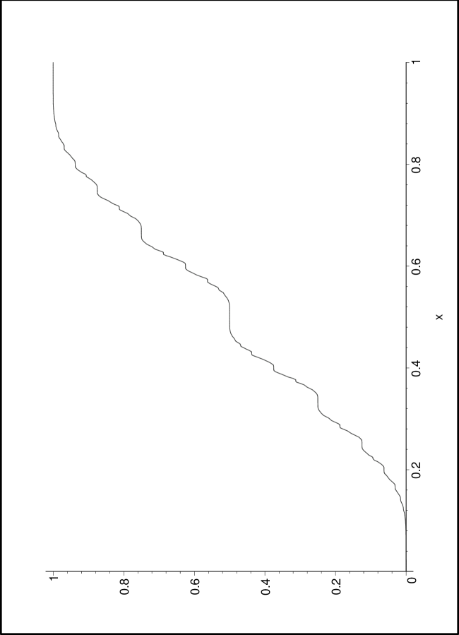
Figure 1: The Minkowski question mark function

In 1943 Raphaël Salem posed a problem about the Fourier coefficients of Minkowski’s question mark function:

$$\alpha_{n}=\int_{0}^{1}e^{2in\pi x}\,dq(x).$$

The Riemann-Lebesgue lemma tells us that Fourier coefficients of an absolutely continuous measure on $[0,1]$ tend to zero. The Minkowski question mark function is singularly continuous, so one cannot use the Riemann-Lebesgue lemma. Nevertheless, the support of $q$ is the full interval $[0,1]$ and it was proved by Salem [27] that $q$ is Hölder continuous of order $\alpha=\log 2/(2\log\frac{\sqrt{5}+1}{2})=0.7202$. Furthermore, Salem showed that

$$\lim_{n\to\infty}\frac{1}{n}\sum_{k=0}^{n}|\alpha_{k}|=\mathcal{O}(n^{-\alpha/2}),$$

so that $\alpha_{n}$ converges to zero on the average and there is the possibility that $\alpha_{n}\to 0$. This is the problem posed by Raphaël Salem [27]: do the Fourier coefficients of the Minkowski question mark function converge to 0? This is still an open problem. Giedrius Alkauskas [2] [3] already investigated this extensively by both numerical and analytical methods.

Our interest in this paper is in the orthonormal polynomials for the Minkowski question mark function:

$$\int_{0}^{1}p_{n}(x)p_{m}(x)\,dq(x)=\delta_{m,n},$$

where $p_{n}(x)=\gamma_{n}x^{n}+\cdots$ and $\gamma_{n}>0$, with recurrence relation

$$xp_{n}(x)=a_{n+1}p_{n+1}(x)+b_{n}p_{n}(x)+a_{n}p_{n-1}(x),\qquad n\geq 0,$$ (2)

with $p_{0}=1$ and $p_{-1}=0$, and in particular we are interested in the asymptotic behavior of the recurrence coefficients $(a_{n})_{n\geq 1}$ and $(b_{n})_{n\geq 0}$. Rakhmanov’s theorem [25] [26] tells us that for an absolutely continuous measure $\mu$ on $[0,1]$ for which $\mu^{\prime}>0$ almost everywhere on $[0,1]$, one has $a_{n}\to 1/4$ and $b_{n}\to 1/2$ as $n\to\infty$. In our case $q^{\prime}=0$ almost everywhere, so one cannot use Rakhmanov’s theorem to deduce the asymptotic behavior of the recurrence coefficients. However, it is known (see, e.g., [21, 32, 29]) that there exist discrete measures and continuous singular measures on $[0,1]$ for which the recurrence coefficients have the behavior $b_{n}\to 1/2$ and $a_{n}\to 1/4$ as $n\to\infty$, so that they are in the Nevai class $M(\frac{1}{2},\frac{1}{4})$.

Definition 1.

The Nevai class $M(b,a)$ consists of all positive measures on the real line for which the orthogonal polynomials have recurrence coefficients satisfying

$$\lim_{n\to\infty}a_{n}=a,\qquad\lim_{n\to\infty}b_{n}=b.$$

It is well known that measures $\mu\in M(b,a)$ have essential spectrum $[b-2a,b+2a]$, i.e., the support of $\mu$ is $[b-2a,b+2a]\cup E$, where $E$ is at most countable and the accumulation points can only be at $b\pm 2a$ (Blumenthal’s theorem, see, e.g., [24, Thm. 7 on p. 23], [31, §5]).

Our first problem is to find out whether the Minkowski question mark function is such a singular continuous function for which the recurrence coefficients are in the Nevai class (for the interval $[0,1]$), i.e., is the following asymptotic behavior true

$$\lim_{n\to\infty}a_{n}=\frac{1}{4},\quad\lim_{n\to\infty}b_{n}=\frac{1}{2}\ ?$$

The symmetry of $q$ around the point $1/2$

$$q(x)=1-q(1-x),\qquad x\in[0,1],$$

already implies that $b_{n}=1/2$ for all $n\in\mathbb{N}$, so the main problem is to find the asymptotic behavior of the recurrence coefficients $(a_{n})_{n\geq 1}$. We will investigate this numerically. In Section 2 we will use the discretized Stieltjes-Gautschi method to compute the recurrence coefficients by approximating the question mark function by a discrete measure which is the empirical distribution function of the Minkowski sequence $\mathcal{M}_{N}$ for various values of $N$. In Section 3 we will use the moments of the question mark function to compute the recurrence coefficients, using the Chebyshev algorithm. In Section 4 we will compare both methods and our conclusion is that the orthogonal polynomials for the question mark function are probably not in Nevai’s class for the interval $[0,1]$.

A second problem is whether the Minkowski question mark function induces a regular measure on $[0,1]$ in the sense of Ullman-Stahl-Totik. Regular measures in the theory of general orthogonal polynomials are those measures for which the asymptotic zero distribution and the $n$th root asymptotics of the leading coefficient $\gamma_{n}$ of the orthonormal polynomial $p_{n}$ is given in terms of the equilibrium measure and the capacity of the support $S_{\mu}$ [30, Def. 1.7 on p. 123], [28, Def. 3.1.2 on p. 61].

Definition 2.

A positive Borel measure $\mu$ on the real line with compact support $S_{\mu}$ is a regular measure if

$$\lim_{n\to\infty}\gamma_{n}^{-1/n}=\textup{cap}(S_{\mu}),$$

where $\textup{cap}(S_{\mu})$ is the logarithmic capacity of $S_{\mu}$, or, equivalently, the zeros $x_{1,n}<x_{2,n}<\cdots<x_{n,n}$ of $p_{n}$ have the behavior

$$\lim_{n\to\infty}\frac{1}{n}\sum_{k=1}^{n}f(x_{k,n})=\int_{S_{\mu}}f(x)\,d\mu_{e}(x)$$

for every continuous function on $S_{\mu}$, where $\mu_{e}$ is the equilibrium measure for the set $S_{\mu}$.

The capacity of an interval $[a,b]$ is given by $(b-a)/4$, so our problem is: does the following asymptotic behavior hold

$$\lim_{n\to\infty}\gamma_{n}^{-1/n}=\frac{1}{4}\ ?$$

By comparing the coefficient of $x^{n+1}$ in the recurrence relation (2) one finds the well-known relation $a_{n+1}=\gamma_{n}/\gamma_{n+1}$, so that

$$a_{1}a_{2}a_{3}\cdots a_{n}=\frac{\gamma_{0}}{\gamma_{n}},$$

and the problem then is to find whether the geometric mean of the recurrence coefficients converges to $1/4$:

$$\lim_{n\to\infty}(a_{1}a_{2}\cdots a_{n})^{1/n}=\frac{1}{4}\ ?$$

Of course, when $a_{n}\to 1/4$, i.e., when the recurrence coefficients are in the Nevai class for the interval $[0,1]$, then the geometric mean also converges to $1/4$. However, as we mentioned earlier, the numerical experiments in Sections 2 and 3 indicate that the recurrence coefficients probably do not converge to $1/4$, but then it is still possible that the geometric mean converges to $1/4$. Our numerical results in Section 3 however indicate that this is not the case and that the geometric mean seems to converge to a value less than $1/4$.

2 The discretized Stieltjes-Gautschi method

The computation of the recurrence coefficients of the orthogonal polynomials with the question mark function requires that we need to be able to integrate polynomials using the measure induced by $q$. This is not easy since the Minkowski question mark function is either defined by a limiting process or by a series involving continued fraction coefficients. We therefore will compute approximate values of the recurrence coefficients using a discretized version of the Stieltjes method, which was introduced by W. Gautschi, see, e.g., [16, §2.2], [17]. The idea is to use a discrete distribution function $q_{N}$ (with finitely many points of increase) which converges weakly to the Minkowski question mark function and to compute the recurrence coefficients $(a_{n,N})_{n\geq 1}$ and $(b_{n,N})_{n\geq 0}$ for the orthogonal polynomials for the distribution $q_{N}$. Then

$$\lim_{N\to\infty}a_{n,N}=a_{n},\quad\lim_{N\to\infty}b_{n,N}=b_{n},$$ (3)

where $(a_{n})_{n\geq 1}$ and $(b_{n})_{n\geq 0}$ are the recurrence coefficients of the orthogonal polynomials for the limiting distribution $q$, so that the recurrence coefficients of the discrete orthogonal polynomials are approximations of the recurrence coefficients of the orthogonal polynomials for the question mark function. The main advantage is that the computations for the discrete measure only require matrix computations and can therefore be easily done.

Rather than using the orthonormal polynomials, we will be using the monic orthogonal polynomials $P_{n}(x)=p_{n}(x)/\gamma_{n}$. These monic orthogonal polynomials satisfy the recurrence relation

$$P_{n+1}(x)=(x-b_{n})P_{n}(x)-a_{n}^{2}P_{n-1}(x),\qquad n\geq 0,$$ (4)

with $P_{0}=1$ and $P_{-1}=0$. In particular we will compute the squared recurrence coefficients $(a_{n}^{2})_{n\geq 1}$. There is no need to compute the recurrence coefficients $(b_{n})_{n\geq 0}$ since the symmetry of $q$ around $1/2$ implies that $b_{n}=1/2$ for all $n\geq 0$.

We have chosen to take for $q_{N}$ the empirical distribution function for the points in the Minkowski sequence $\mathcal{M}_{N}$. This means that we take

$$q_{N}(x)=\frac{1}{m_{N}}\#\{a/b\in\mathcal{M}_{N}\ |\ a/b\leq x\},$$

where $m_{N}=2^{N-1}+1$ is the number of points in $\mathcal{M}_{N}$. The measure induced by $q_{N}$ is supported on the Minkowski sequence $\mathcal{M}_{N}$ and each point has equal mass $1/m_{N}$. The corresponding measure can be written as

$$\frac{1}{m_{N}}\sum_{a/b\in\mathcal{M}_{N}}\delta_{a/b},$$

where $\delta_{c}$ is the Dirac measure at $c$. It is not so difficult to see that this discrete measure converges weakly to the measure induced by the Minkowski question mark function and in fact

$$\lim_{N\to\infty}q_{N}(x)=q(x),$$

uniformly on $[0,1]$ (see, e.g., [1, §2.1]). We have used these empirical distribution functions for $N=10$ up to $N=18$ (hence discrete measures with 513, 1025, 2049, 4097, 8193, 16385, 32769, 65537, and 131073 points) to compute the first 100 recurrence coefficients. The discrete measures are symmetric with respect to the point $1/2$, hence automatically $b_{n,N}=1/2$ for $0\leq n\leq 2^{N-1}$, so the main problem is to compute the recurrence coefficients $a_{n,N}^{2}$ and since we are only interested in the limit for $N\to\infty$, we restrict our attention to $1\leq n\leq 100$. First we need to find all the points in the set $\mathcal{M}_{N}$, which is easily done by the following procedure in Maple, using the packages LinearAlgebra and ArrayTools:

minkseq:=proc(N)
  local s,k,i;
  s:=Vector[row](2^{N-1}+1,fill=1);
  s[1]:=0;
  s[2]:=1;
  for i from 2 to n do
     for k to 2^(i-2) do
        s[2^(i-2)+k+1]:=(numer(s[k])+numer(s[k+1]))
                        /(denom(s[k])+denom(s[k+1]))
     end do;
     s=:sort(s)
  end do;
  s
end proc;

The weights corresponding to the points in $\mathcal{M}_{N}$ are all equal to $1/(2^{N-1}+1)$. Then we used the discretized Stieltjes-Gautschi method as is described in [19, §4.1 on p. 34] and implemented in the algorithm stieltjes.m [18]. We have made our computations in Maple in a precision given by Digits:=100. The resulting recurrence coefficients $a_{n,N}^{2}$ are given in Figures 2–4.

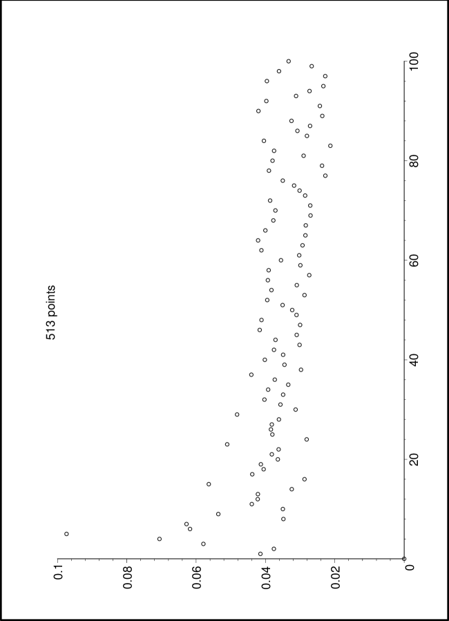
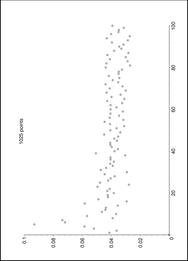
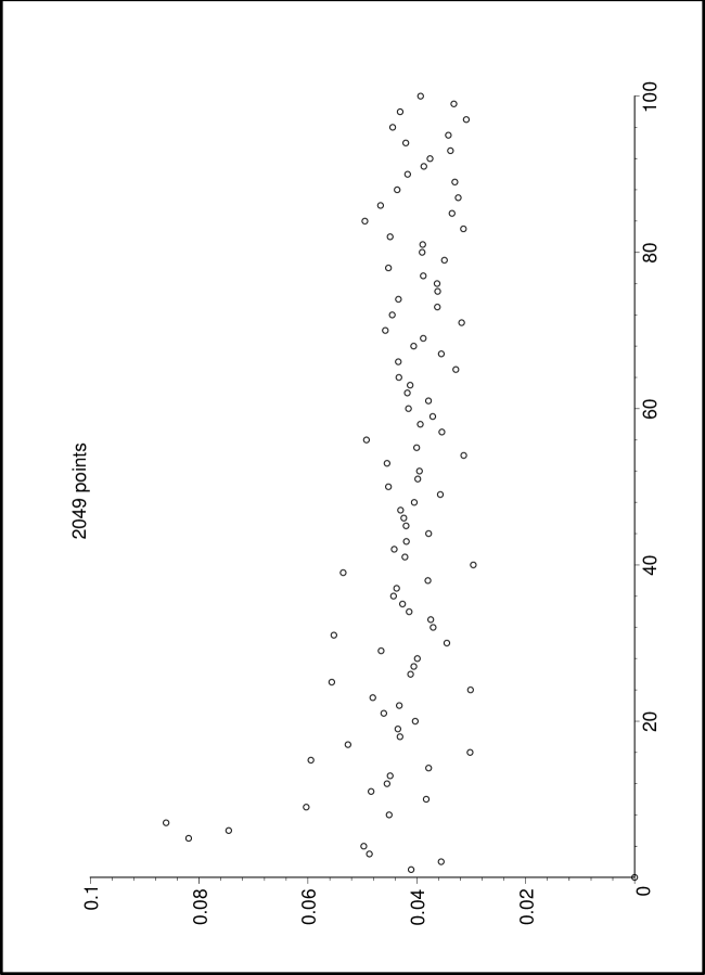
Figure 2: The recurrence coefficients $a_{n,N}^{2}$ for $N=10,11,12$

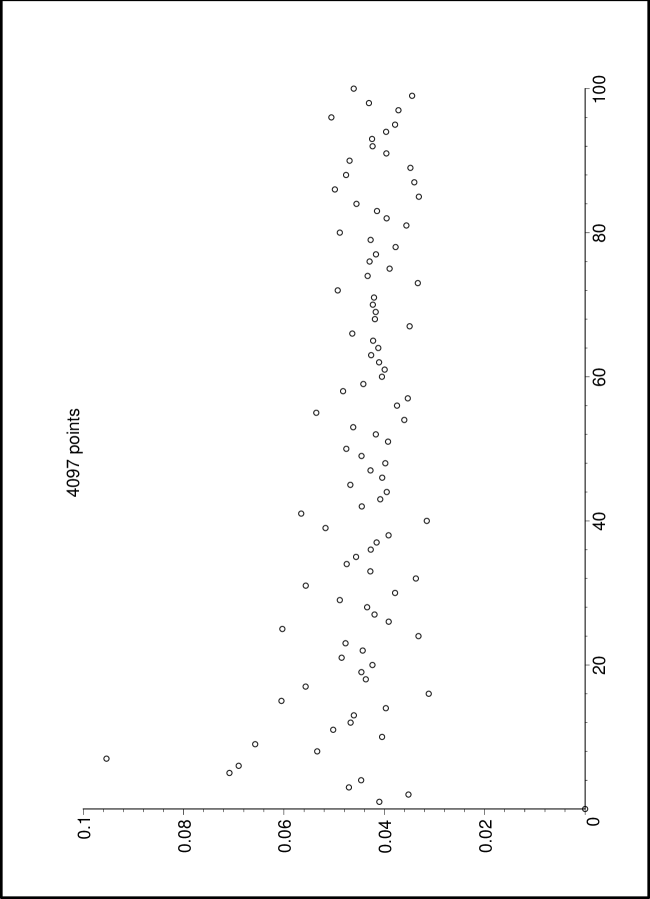
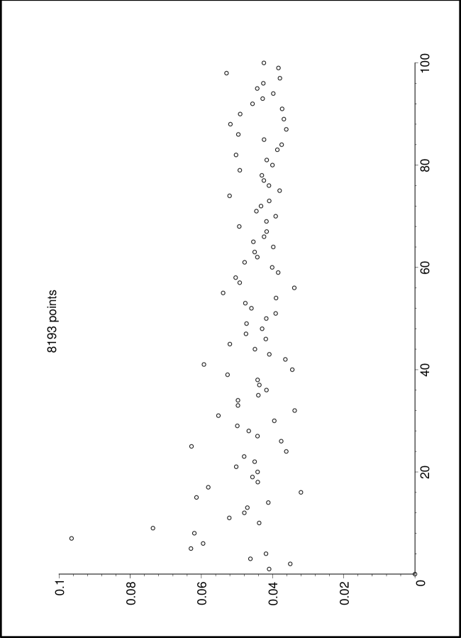
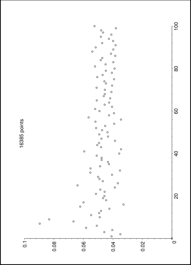
Figure 3: The recurrence coefficients $a_{n,N}^{2}$ for $N=13,14,15$

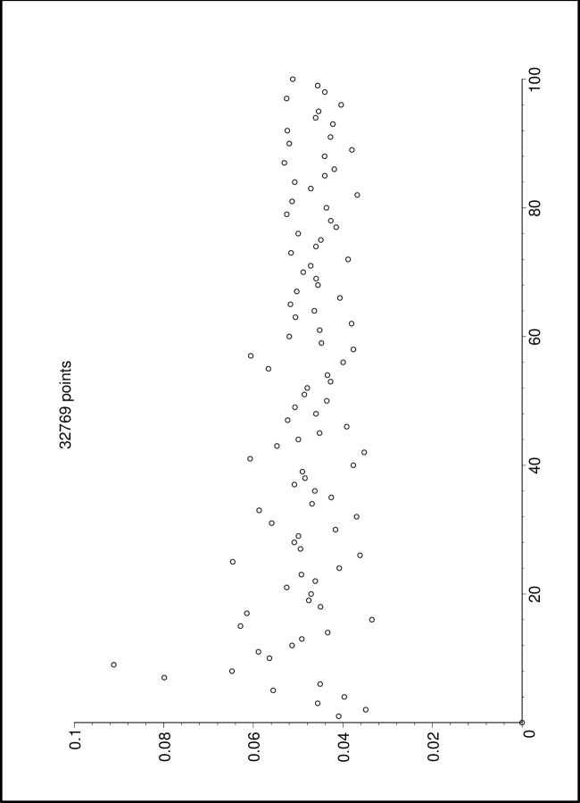
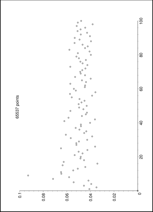
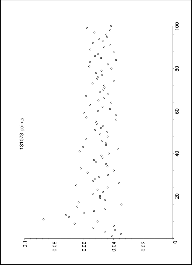
Figure 4: The recurrence coefficients $a_{n,N}^{2}$ for $N=16,17,18$

Even though the figures all show a similar behavior, they give different approximations for the recurrence coefficients of the orthogonal polynomials for the question mark function. The values are lying around $0.04$ to $0.05$ but there is a large value of $a_{n,N}^{2}$ (larger than 0.08) near the beginning which changes significantly in size and position when $N$ changes, see Table 1.

$a_{5,10}^{2}$	0.0973813815
$a_{5,11}^{2}$	0.0929448256
$a_{7,12}^{2}$	0.0860780825
$a_{7,13}^{2}$	0.0953811702
$a_{7,14}^{2}$	0.0964882611
$a_{7,15}^{2}$	0.0896426756
$a_{9,16}^{2}$	0.0911621120
$a_{9,17}^{2}$	0.0927763299
$a_{9,18}^{2}$	0.0872304015

Table 1: Largest values of $a_{n,N}^{2}$

3 Moments

In this section we will compute the recurrence coefficients by using the moments of the Minkowski question mark function. We have computed the moments using a method suggested by G. Alkauskas [4] [5]. We use the relation

$$m_{s}=\sum_{k=0}^{\infty}(-1)^{k}c_{k+s}\binom{k+s-1}{k}m_{k},\qquad s\geq 1,$$ (5)

where

$$c_{k}=\sum_{n=1}^{\infty}\frac{1}{2^{n}n^{k}},$$

then truncate the sum for $c_{n}$ to 400 terms and truncate the sum in (5) to 500 terms, so that it becomes a linear system of equations for the moments, with initial moment $m_{0}=1$. The error we make by truncating the sum for $c_{k}$ is

$$\sum_{n=401}^{\infty}\frac{1}{2^{n}n^{k}}<\sum_{n=401}^{\infty}\frac{1}{2^{n}}=2^{-400}\approx 0.387\ 10^{-120},$$

hence the $c_{k}$ are accurately computed up to 120 decimals. In Maple we used Digits:=400 and we obtained the moments as given (with 50 decimals) in A. The condition number of the matrix for this linear system is quite high (of the order $10^{435}$) so that the results must be treated with some suspicion, even with using high accuracy. The first moment $m_{1}$ is 1/2 and hence this value can be used to check the accuracy of the method: the computed value of $m_{1}$ was correct up to 93 decimals ($m_{1}=0.4999999\ldots$, with 92 nines). The accuracy seems to decrease for the higher moments. Our value of $m_{100}$ is

$$m_{100}=.000000444593386091498$$

which differs slightly from the value $0.0000004445933003$ in [4, p. 366].

An exact formula for the moments is given in [6]. This formula is not very suitable for computing the moments, but another infinite system of equations was mentioned in [7, p. 364]. The relation is

$$m_{s}=\sum_{k=0}^{\infty}d_{k+s}\binom{k+s-1}{k}m_{k},\quad s\geq 1,$$ (6)

where

$$d_{k}=2\sum_{n=2}^{\infty}\frac{1}{2^{n}n^{k}}=2c_{k}-1.$$

This relation can be proved in a similar way as Proposition 5 in [6] but using another functional equation for the moment generating function

$$G(z)=\sum_{k=1}^{\infty}m_{k}z^{k-1},$$

than the one used in the proof of (5), namely [6, Eq. (12)]

$$G(z)=-\frac{1}{1-z}-\frac{1}{(1-z)^{2}}G\left(\frac{1}{1-z}\right)+2G(z+1).$$

If we truncate the sum in (6) to 500 terms, then the linear system has a matrix with only positive terms and the condition number 2.97 is low. The value of $m_{1}$ was correct up to $31$ decimals ($m_{1}=0.4999999\ldots$, with 30 nines), which is less than using the linear system (5), but now this error is of the same magnitude for all moments. In fact we do get the same value for the moment $m_{100}$ as given higher. We believe that the reason why (6) gives less accurate results than (5) is that the truncation of the infinite system of equations to a matrix of size 500 leaves the error

$$\sum_{k=501}^{\infty}(-1)^{k}c_{k+s}\binom{k+s-1}{k}m_{k}$$

for the first system which, due to the oscillating terms in the sum, is much less than the error

$$\sum_{k=501}^{\infty}d_{k+s}\binom{k+s-1}{k}m_{k}$$

for the second system, which contains only positive terms. So even though the matrix of the second system is better conditioned than the matrix of the first system, the results of the first system give more accurate approximations to the moments.

Next, we used these moments to compute the recurrence coefficients in the three-term recurrence relation

$$P_{n+1}(x)=(x-b_{n})P_{n}(x)-a_{n}^{2}P_{n-1}(x)$$

of the monic orthogonal polynomials for Minkowski’s question mark function. We used the Chebyshev algorithm (with the ordinary moments, see [16, Algorithm 2.1 on p. 77]). It is well known that the mapping from moments $(m_{n})_{n\geq 0}$ to the recurrence coefficients $(a_{n+1}^{2},b_{n})_{n\geq 0}$ is badly conditioned, see, e.g., [16, §2.1.6]. This is the reason why we used high precision (Digits:=400) in our calculations. Recall that, due to the symmetry, all the recurrence coefficients $b_{n}$ are constant: $b_{n}=1/2$. This was useful to check the accuracy of our computations. We observed that our computed values of $b_{n}$ were correct to 23 decimal places up to $b_{40}$ but then slowly started to show errors, with $b_{53}$ a negative value, which is impossible. Therefore we listed and plotted the computed values of $a_{n}^{2}$ only up to $a_{40}^{2}$ in Table 2 and Figure 5.

$k$	$b_{k}$	$a_{k}^{2}$
0	0.5
1	0.5	0.040926476429308736381
2	0.5	0.034881265506134342903
3	0.5	0.045430415370805808038
4	0.5	0.038973377115288248098
5	0.5	0.052863907245188596784
6	0.5	0.037955175327144719607
7	0.5	0.059731637094523918352
8	0.5	0.038238400877758730555
9	0.5	0.058672115522904960765
10	0.5	0.046255346737208862213
11	0.5	0.050520824434494850803
12	0.5	0.051910925145095030363
13	0.5	0.056489563093038456301
14	0.5	0.040208992500495472293
15	0.5	0.071218137450141992615
16	0.5	0.039427602611174900647
17	0.5	0.059396186789821055700
18	0.5	0.053652031489601189600
19	0.5	0.053884790282064402379
20	0.5	0.050381653151077022836
21	0.5	0.057911359198380156348
22	0.5	0.053527412587600219313
23	0.5	0.057334758849746482997
24	0.5	0.044067432839352949172
25	0.5	0.073234222409597016726
26	0.5	0.043818059541906812748
27	0.5	0.056063579773800371687
28	0.5	0.058703247843561897668
29	0.5	0.057201243688393241195
30	0.5	0.049069569275476665894
31	0.5	0.064554576616699275413
32	0.5	0.045732073443752859070
33	0.5	0.069343850504209381053
34	0.5	0.049351815705867268360
35	0.5	0.053031677464673738708
36	0.5	0.061496568432752989923
37	0.5	0.058321435643186334303
38	0.5	0.052208175547033955364
39	0.5	0.056607898016942758422
40	0.5	0.055895931809777873999

Table 2: The recurrence coefficients $b_{n}$ and $a_{n}^{2}$

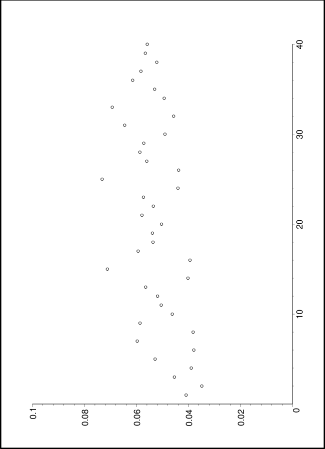
Figure 5: The recurrence coefficients $a_{n}^{2}$

In order to check whether the question mark function induces a regular measure on $[0,1]$, we need to compute $\gamma_{n}^{-1/n}$, where

$$\frac{1}{\gamma_{n}^{2}}=\int_{0}^{1}P_{n}^{2}(x)\,dq(x)=a_{1}^{2}a_{2}^{2}\cdots a_{n}^{2}.$$

For a regular measure on $[0,1]$ one has

$$\lim_{n\to\infty}\left(\frac{1}{\gamma_{n}}\right)^{1/n}=\frac{1}{4},$$

where $1/4$ is the logarithmic capacity of the interval $[0,1]$. It is more convenient to compute $\gamma_{n}^{-2/n}$ since we are really computing the squared recurrence coefficients $a_{n}^{2}$. Our computations (see Table 3) indicate that the sequence $(a_{1}^{2}a_{2}^{2}\cdots a_{n}^{2})^{1/n}$ may indeed be converging, but the limit is near $0.052$ instead of $(1/4)^{2}=1/16=0.0625$.

$k$	$(a_{1}^{2}a_{2}^{2}\cdots a_{k}^{2})^{1/k}$
1	0.040926476429308736381
2	0.037783161468586334476
3	0.040177332455719534022
4	0.039872900960755211548
5	0.042186560554634906505
6	0.041449910727599868208
7	0.043670914641443765852
8	0.042951735555887041699
9	0.044466283404646215085
10	0.044642030777323595493
11	0.045146924287480657337
12	0.045675227441320883038
13	0.046427976597463213256
14	0.045953497782193798426
15	0.047315493717202662999
16	0.046779242858071064616
17	0.047440963915026139792
18	0.047766342240858080778
19	0.048070312391450962315
20	0.048183319646452786085
21	0.048607122313805874900
22	0.048820630103435556238
23	0.049163047752620715919
24	0.048939412842737333783
25	0.049734867738244766161
26	0.049493171229376460057
27	0.049722196075856275919
28	0.050017931134405002549
29	0.050249919542639211311
30	0.050210120837211061076
31	0.050618791840573811015
32	0.050458453441009796727
33	0.050946927334564490546
34	0.050899284439881664328
35	0.050959003303570963593
36	0.051225761593643949404
37	0.051405681461085926182
38	0.051426640855254603168
39	0.051553375093489825709
40	0.051657713625567224389

Table 3: The values of $\gamma_{n}^{-2/n}=(a_{1}^{2}a_{2}^{2}\cdots a_{n}^{2})^{1/n}$.

4 Conclusion

4.1 The discretized Stieltjes-Gautschi method

When we compare the values of $a_{n,N}^{2}$ obtained in Section 2 with the values obtained in Section 3 (using the moments of $q$), see Figure 5, only the first five recurrence coefficients $a_{n,18}^{2}$ are close to the actual values. The reason that we don’t get accurate results for the $a_{n}^{2}$ is that the $a_{n,N}^{2}$ are approximations for the $a_{n}^{2}$ and that one needs to take the limit $N\to\infty$ to get the desired recurrence coefficients. The discrete distribution functions $q_{N}$ converge slowly to the Minkowski question mark function. In fact, it is known that

$$\max_{x\in[0,1]}|q_{N}(x)-q(x)|=\frac{1}{2^{N-1}+1},$$

hence the error $\|q_{N}-q\|_{\infty}$ is of the order $1/m_{N}$, where $m_{N}$ is the number of points in the support of the discrete measure $q_{N}$. The discrete approximation $q_{N}(x)$ for $x$ near $0$ and near $1$ is quite poor since the first point in $\mathcal{M}_{N}$ (after $0$) is $1/N$ and the largest point (before 1) is $(N-1)/N$. These single points have the task to represent $q$ on an interval of reasonable large size compared to the number of points which are available. The computations are in fact quite accurate for the recurrence coefficients $a_{n,N}^{2}$ of the discrete orthogonal polynomials, but the convergence in (3) is rather slow (except, of course, for $b_{n,N}$).

4.2 Behavior of the recurrence coefficients

If we compute the recurrence coefficients $(a_{k}^{2})_{1\leq k\leq n}$ and $(b_{k})_{0\leq k\leq n}$ from the moments $(m_{k})_{0\leq k\leq 2n}$, then we can’t compute many coefficients since the mapping from moments to recurrence coefficients becomes ill-conditioned at an exponential rate in $n$. The use of modified moments

$$\hat{m}_{n}=\int_{0}^{1}r_{n}(x)\,dq(x),$$

where $(r_{n})_{n\in\mathbb{N}}$ is a sequence of known polynomials, sometimes leads to a better conditioned mapping from modified moments to recurrence coefficients, in particular when the polynomials $(r_{n})_{n\in\mathbb{N}}$ are already close to the polynomials $(p_{n})_{n\in\mathbb{N}}$ for which we are computing the recurrence coefficients. Unfortunately no such system of polynomials seems to be available and our attempts to use the Chebyshev polynomials on $[0,1]$ lead to a similar ill-conditioned problem. So we are stuck with the regular moments and high precision arithmetic, which allowed us to compute 40 recurrence coefficients $a_{n}^{2}$ reliably. The reliability was checked by using the recurrence coefficients $b_{k}$ as control variables, since we know that they are all constant and equal to 1/2: errors in the computed values of $b_{k}$ for $k>n_{0}$ certainly indicate that the corresponding $a_{k}^{2}$ for $k>n_{0}$ are not reliable. On the other hand, if the $b_{k}$ are computed accurately for $k\leq n_{0}$ then one may reasonably assume that the $a_{k}^{2}$ are also accurate for $k\leq n_{0}$, except possibly the last one.

Of course, 40 recurrence coefficients are not really enough to say something about the asymptotic behavior of the recurrence coefficients. Nevertheless Figure 5 doesn’t give the impression that the recurrence coefficients are converging. The recurrence coefficients vary somewhat between $0.04$ and $0.06$ with some higher values. The average of the recurrence coefficients $a_{n}^{2}$ for $1\leq 40$ is $0.05246234283$ which is not close to $1/16=0.0625$. Hence, based on our numerical evidence, we conclude that the recurrence coefficients $(a_{n}^{2})_{n}$ do not converge, and even their averages do not seem to converge to $1/16$. This means that Minkowski’s question mark function does not give orthogonal polynomials in the Nevai class $M(\frac{1}{2},\frac{1}{4})$, and most likely not in any other Nevai class $M(\frac{1}{2},a)$.

4.3 Does $q$ induce a regular measure?

The oscillating nature of the recurrence coefficients $(a_{n}^{2})_{n\geq 1}$ still leaves open the possibility that the geometric mean $(a_{1}^{2}a_{2}^{2}\cdots a_{n}^{2})^{1/n}$ converges. Our numerical experiments, with $1\leq n\leq 40$, indicate that the geometric mean may be converging but that the limit is less than $1/16=0.0625$, see Table 3. Hence our numerical evidence leads to the conclusion that the question mark function does not induce a regular measure on $[0,1]$.

In general it is known that

$$c_{\mu}\leq\liminf_{n\to\infty}\gamma_{n}^{-1/n}\leq\limsup_{n\to\infty}\gamma_{n}^{-1/n}\leq\textup{cap}(S_{\mu}),$$

where $S_{\mu}$ is the support of the orthogonality measure $\mu$ and $c_{\mu}$ is the minimal carrier capacity of $\mu$,

$$c_{\mu}=\inf\{\textup{cap}(B)\ |\ B\textrm{ is a bounded Borel set and }\mu(\mathbb{R}\setminus B)=0\}.$$

Hence if the Minkowski question mark function does not induce a regular measure $\mu$ on $[0,1]$, then this implies that the minimal carrier capacity of the question mark function is less than $1/4$. The reason why $q$ does not induce a regular measure is probably that the support $[0,1]$ contains intervals with exponentially small measure. Indeed, one easily finds

$$q\left(\frac{1}{n}\right)-q(0)=\frac{1}{2^{n-1}},\qquad q(1)-q\left(1-\frac{1}{n}\right)=\frac{1}{2^{n-1}},$$

$$q\left(\frac{1}{2}+\frac{1}{4n}\right)-q\left(\frac{1}{2}-\frac{1}{4n}\right)=\frac{3}{2}\frac{1}{2^{n}},$$

so that the intervals $[0,\frac{1}{n}]$, $[\frac{n-1}{n},1]$ and $[\frac{1}{2}-\frac{1}{4n},\frac{1}{2}+\frac{1}{4n}]$ of length $\mathcal{O}(1/n)$ have measure proportional to $1/2^{n}$. These intervals reappear all over the interval $[0,1]$ because of the self-similar nature of $q$, expressed by (1). Hence, the support of the measure induced by the question mark function behaves like a subset of $[0,1]$ with gaps and for measures with a support containing gaps, the recurrence coefficients show much more oscillating or chaotic behavior. The minimal carrier capacity would be less than the capacity of $[0,1]$ due to these gaps which have exponentially small measure.

4.4 Open problems

Many open problems remain for the orthogonal polynomials related to the question mark function [10]. To name a few:

• Is there any structure in the seemingly chaotic behavior of the recurrence coefficients? In particular it would be nice to know whether the coefficients $a_{n}^{2}$ are almost periodic. To answer this question it would be necessary to calculate the mean of the coefficients and then to look for oscillations about this mean. This would require many more coefficients than available right now.

• Can one determine

  $$\liminf_{n\to\infty}a_{n}^{2},\quad\limsup_{n\to\infty}a_{n}^{2}\ ?$$

• Does the geometric mean

  $$\lim_{n\to\infty}(a_{1}a_{2}\ldots a_{n})^{2/n}$$

  exist?

• Is this limit (if it exists) equal to the minimal carrier capacity of the measure induced by the question mark function?

The question mark function is a reasonably simple singularly continuous measure which, next to the well known Cantor measure, is useful to investigate how the recurrence coefficients of orthogonal polynomials with singular continuous measure behave. This paper is the first in which the Minkowski question mark function is considered in the context of orthogonal polynomials. Earlier there have been a number of papers dealing with the recurrence coefficients of orthogonal polynomials for the Cantor measure, and for these many more recurrence coefficients have been investigated, see e.g., the work of G. Mantica [22], H.-J. Fischer [15] and the recent work of Heilman, Owrutsky and Strichartz [20] on orthogonal polynomials with self-similar measures.

A very relevant singular continuous measure is the equilibrium measure for the Julia set of the iteration of a polynomial $T$, such as $T(x)=x^{2}-c$, with $c>2$. Such a Julia set is of the same nature as the Cantor set, where one iteratively removes intervals from a given interval. The orthogonal polynomials for such a singular measure have been analyzed in detail by Barnsley, Geronimo, Harrington [8], Bellissard, Bessis, Moussa [9], Bessis, Geronimo, Moussa [11] and Bessis, Mehta, Moussa [12]. One of their results is that the subsequence $P_{2^{n}}(x)$ of the orthogonal polynomials is explicitly given by the $n$-th iterate of the given polynomial $T(x)$ and that the recurrence coefficients satisfy some non-linear relations, from which one can deduce that the recurrence coefficients are limit periodic for a large class of polynomials $T$. It would be nice to obtain such results for the Minkowski question mark function. However, the self-similarity of the question mark function, as described by (1), involves rational functions so that (orthogonal) polynomials composed with rational functions lead to rational functions and hence the polynomial nature is not preserved by the mappings in the iterated function system.

Acknowledgement

We thank S. Yakubovich for bringing the Minkowski question mark function to our attention. This research was supported by KU Leuven research grant OT/12/073, FWO grant G.0427.09 and the Belgian Interuniversity Attraction Poles Programme P7/18.

Appendix A Moments

$k$	$m_{k}$
1	0.50000000000000000000000000000000000000000000000000
2	0.29092647642930873638069776273912029008043710219559
3	0.18638971464396310457104664410868043512065565329339
4	0.12699225840744313520289222788021163884118514576173
5	0.090164454945335997055486162852728371901870108915328
6	0.065928162577472341926815287122643139097250419686219
7	0.049294310463767495715873019738162192824596016540408
8	0.037518711852048335539887123885001326828330311845185
9	0.028979622034097514125202534817631105526453454918480
10	0.022665858176292038567084595433830909709028113615601
11	0.017920859234922559709620674061965959387422365122601
12	0.014304689510828028713327933529010923388486775628519
13	0.011515014023688037216614175868946822321198574437066
14	0.0093396445516456630408229433763950525836249376062925
15	0.0076269557590972324137284663579204452441313886605484
16	0.0062668792729955855181245666105463942184539549010276
17	0.0051783877867685200880408849955806484581000333322566
18	0.0043010785465847754710770555353762470229805125766226
19	0.0035894093787684071613366998806631220004089279356802
20	0.0030086867071149232599754021703205599242915788661537
21	0.0025322317634222266277036639307882264778052530156116
22	0.0021393519928752509332902769549514723550086345056961
23	0.0018138708773921687964413975361770115813330394837942
24	0.0015430503000888974750639610156922661098154179170794
25	0.0013167923220646751068501044957069765425398359511571
26	0.0011270421715775897395157816468683456633974505562164
27	0.00096733770677037783561122437105791592882537796051057
28	0.00083246658220639104473557479405732069610975267509581
29	0.00071820335559030841469949022408376381202557302200995
30	0.00062110644645096567556056888154034901542203410280702
31	0.00053836027103037905202629197075705905383821217884329
32	0.00046765173455275558510114895133989297915712195884076
33	0.00040707303776263157571881765213893343503728847982982
34	0.00035504477084132941930948314931026013893192071414219
35	0.00031025474516371162917662025303647309624750426315414

$k$	$m_{k}$
36	0.00027160910474659558624707454363471603060022780445456
37	0.00023819307170515894210646197643373870213103110230062
38	0.00020923928922626913333968336609713458623759072879973
39	0.00018410218544426637502507882484141316037994511212385
40	0.00016223713098006110726991119269902592433404152806255
41	0.00014318342992835510310721778791488526305144139896956
42	0.00012655038932266879782766519282463067535339428877894
43	0.00011200587071717784852138503115054268313120729105696
44	0.000099266850721688056248146847039352100867092413446553
45	0.000088091613483408666548718142966352919966384794835161
46	0.000078273273509573469871441756231586836413236191991855
47	0.000069634386611004882448594820251627462598040246563183
48	0.000062022453717890701051430866178792091112759697349794
49	0.000055306159621487594284446897034200886840998808601394
50	0.000049372218434717208976312359496974514537772757968773
51	0.000044122721362726073881354844160254923500862547763273
52	0.000039472901486704070959737735999458212044994283495032
53	0.000035349245666258223798489554957594867788549703093561
54	0.000031687896118933003424939851849986040400796168900580
55	0.000028433294336821167964517994319875407187553962659664
56	0.000025537028219094604542709782295425670986358747374410
57	0.000022956850006417952618424640438139791507342597816299
58	0.000020655838092375878340873282295400282104460092785749
59	0.000018601680291880423863588358493197745228211014253879
60	0.000016766059853447792758997531437488191617648704513657
61	0.000015124128560475439274975373678569160508643322805383
62	0.000013654053796046797396039913645973219220649444564075
63	0.000012336628542866380312339531772945578083278145703849
64	0.000011154935032657469162573155131448984539990112465750
65	0.000010094054210908289421180310562947718378648386875946
66	0.0000091408143945475299648985162271152064510786088610998
67	0.0000082835735137657351740548705254404013142671182635503
68	0.0000075120301789106204917387855457822400686084713220510
69	0.0000068170595271178220756077387776286434567656799242417
70	0.0000061905704040288945388332526110642901215894448069398

References

-
[1]
G. Alkauskas,
Integral transforms of the Minkowski question mark function,
PhD thesis, University of Nottingham, 2008.
http://etheses.nottingham.ac.uk/641/ - [2] G. Alkauskas, The Minkowski function and Salem’s problem, C.R. Math. Acad. Sci. Paris 350 (2012), no. 3–4, 137–140.
- [3] G. Alkauskas, Fourier-Stieltjes coefficients of the Minkowski question mark function, Analytic and Probabilistic Methods in Number Theory, Proceedings of the 5th International Conference in honour of J. Kubilius (Palanga, Lithuania, 4–10 September 2011), 2012, pp. 19–33. arXiv:1008.4014 [math.CA]
- [4] G. Alkauskas, An asymptotic formula for the moments of the Minkowski question mark function in the interval , Lithuanian Math. J. 48, no. 4 (2008), 357–367.
- [5] G. Alkauskas, The Minkowski question mark function: explicit series for the dyadic period function and moments, Math. Comput. 79 (269) (2010), 383–418; Addenda and corrigenda, Math. Comp. 80 (276), (2011), 2445–2454.
- [6] G. Alkauskas, The moments of Minkowski question mark function: the dyadic period function, Glasgow Math. J. 52 (2010), 41–64.
- [7] G. Alkauskas, Semi-regular continued fractions and an exact formula for the moments of the Minkowski question mark function, Ramanujan J. 25 (2011), 359–367.
- [8] M.F. Barnsley, J.S. Geronimo, A.N. Harrington, Almost periodic Jacobi matrices associated with Julia sets for polynomials, Comm. Math. Phys. 99 (1985), no. 3, 303–317.
- [9] J. Bellissard, D. Bessis, P. Moussa, Chaotic states of almost periodic Schrödinger operators, Phys. Rev. Lett. 49 (1982), no. 10, 701–704.
- [10] C. Berg, Open problems, Integral Transforms Spec. Funct. (to appear).
- [11] D. Bessis, J.S. Geronimo, P. Moussa, Function weighted measures and orthogonal polynomials on Julia sets, Constr. Approx. 4 (1988), no. 2, 157–173.
- [12] D. Bessis, M.L. Mehta, P. Moussa, Orthogonal polynomials on a family of Cantor sets and the problem of iterations of quadratic mappings, Lett. Math. Phys. 6 (1982), no. 2, 123–140.
- [13] A. Denjoy, Sur quelques points de la théorie des fonctions, C.R. Acad. Sci. Paris 194 (1932), 44–46.
- [14] A. Denjoy, Sur une fonction réelle de Minkowski, J. Math. Pures Appl. 17 (1938), 105–151.
- [15] H.-J. Fischer, Recurrence coefficients of orthogonal polynomials with respect to some self-similar singular distributions, Z. Anal. Anwendungen 14 (1995), no. 1, 141–155.
- [16] Walter Gautschi, Orthogonal Polynomials: Computation and Approximation, Oxford University Press, 2004.
- [17] W. Gautschi, On generating orthogonal polynomials, SIAM J. Sci. Statist. Comput. 3 (1982), 289–317.
-
[18]
W. Gautschi,
OPQ: matlab suite for generating orthogonal polynomials and related quadrature rules.
http://www.cs.purdue.edu/archives/2002/wxg/codes/ - [19] W. Gautschi, Algorithm 726: ORTHPOL – a package of routines for generating orthogonal polynomials and Gauss-type quadrature rules, ACM Trans. Math. Software 20 (1994), 21–62.
- [20] S.M. Heilman, P. Owrutsky, R.S. Strichartz, Orthogonal polynomials with respect to self-similar measures, Exp. Math. 20 (2011), no. 3, 238–259.
- [21] D.S. Lubinsky, Singularly continuous measures in Nevai’s class , Proc. Amer. Math. Soc. 111 (1991), 413–420.
- [22] G. Mantica, A stable Stieltjes technique for computing orthogonal polynomials and Jacobi matrices associated with a class of singular measures, Constr. Approx. 12 (1996), no. 4, 509–530.
- [23] H. Minkowski, Zur Geometrie der Zahlen, Verhandlungen des III. Internationalen Mathematiker-Kongresses, Heidelberg, 1904, pp. 164–173.
- [24] P.G. Nevai, Orthogonal Polynomials, Mem. Amer. Math. Soc. 18 (1979), no. 213, v+185 pp.
- [25] E.A. Rakhmanov, On the asymptotics of the ratio of orthogonal polynomials, Mat. Sb. 103 (145) (1977), 237–252 (in Russian); translated in Math. USSR Sb. 32 (1977), 199–213.
- [26] E.A. Rakhmanov, On the asymptotics of the ratio of orthogonal polynomials, II Mat. Sb. 118 (160) (1982), 104–117 (in Russian); translated in Math. USSR Sb. 47 (1983), 105–117.
- [27] R. Salem, On some singular monotonic functions which are strictly increasing, Trans. Amer. Math. Soc. 53 (1943), 427- 439.
- [28] Herbert Stahl, Vilmos Totik, General Orthogonal Polynomials, Encyclopedia of Mathematics and its Applications 43, Cambridge University Press, 1992.
- [29] V. Totik, Orthogonal polynomials with ratio asymptotics, Proc. Amer. Math. Soc. 114 (1992), 491–495.
- [30] J.L. Ullman, On the regular behaviour of orthogonal polynomials, Proc. London Math. Soc. (3), 24 (1972), 119–148.
- [31] W. Van Assche, Compact Jacobi matrices: from Stieltjes to Krein and , Ann. Fac. Sci. Toulouse Math. (6) (1996), Special issue “100 ans après Th.-J. Stieltjes”, pp. 195–215.
- [32] W. Van Assche, A.P. Magnus, Sieved orthogonal polynomials and discrete measures with jumps dense in an interval, Proc. Amer. Math. Soc. 106 (1989), 163–173.