Kepler-9 revisited

Abstract

Aims. Kepler-9 was the first case where transit timing variations have been used to confirm the planets in this system. Following predictions of dramatic TTVs - larger than a week - we re-analyse the system based on the full Kepler data set.

Methods. We re-processed all available data for Kepler-9 removing short and long term trends, measured the times of mid-transit and used those for dynamical analysis of the system.

Results. The newly determined masses and radii of Kepler-9b and -9c change the nature of these planets relative to the one described in Holman et al. 2010 (hereafter H10) with very low, but relatively well charcterised (to better than 7%), bulk densities of 0.18 and 0.14 g cm³ (about 1/3 of the H10 value). We constrain the masses (45.1 and 31.0 M_⊕, for Kepler-9b and -9c respectively) from photometry alone, allowing us to see possible indications for an outer non-transiting planet in the radial velocity data. At $2R_{\oplus}$ Kepler-9d is determined to be larger than suggested before - suggesting that it is a low-mass low-density planet.

Conclusions. The comparison between the H10 analysis and our new analysis suggests that small formal error in the TTV inversion may be misleading if the data does not cover a significant fraction of the interaction time scale.

1 Introduction

Transit timing variations (TTVs) are deviations from strict periodicity in extra solar planetary transits, caused by non-Keplerian forces – usually the interaction with other planets in the system. These TTVs are particularly important in multi-transiting systems since they can allow learning about dynamics in the system, which in turn can confirm the exoplanetary origin of the transit signals with no further observations (e.g. Holman et al. 2010, H10 hereafter, or Xie 2013), and sometimes even allow deriving the planets’ mass from photometry alone (Kepler-87, Ofir et al., 2014). For these reasons TTVs had attracted a lot of attention since they were first predicted by Holman & Murray (2005) and Agol et al. (2005), and especially since they where first observed by H10 in the prototypical Kepler-9 system.

Kepler-9 is prototypical not just because it was the first object detected with TTVs, but also since it is a textbook-like example of TTVs: exhibiting very large TTVs on very deep transits, making the effect abundantly clear. The first study of the Kepler-9 system also included a prediction for the expected TTVs during the following few years (their Figure S4) which included dramatic TTV spanning up to about ${}^{+4}_{-8}d$ relative to the nominal ephemeris, accumulated over long interaction times scales (e.g. $\sim 1000d$ from first maximum to first minimum TTV excursion of Kepler-9c). These very large TTVs are easy to compare to the observed ones in later Kepler data. Indeed by the time we re-analysed this object much more data were available, revealing that the actual TTVs, while still large, were much less extreme than initially predicted. We observed TTV spans of about ${}^{+0.6}_{-0.9}d$ for the same features as above, and TTV time scale about half as long as predicted. These prompted us to revisit the analysis of Kepler-9.

This paper is therfore divided in the following way: in sections §2 and §3 we describe the input data and TTV analysis procedures we used. In §4 we made sure we are able to recover the H10 results when using only the data that was available at the time, showing consistent analysis, which then allowed us to perform a full analysis using the full data set in §5, before discussing the updated analysis in §6.

2 Photometry and light curve modeling

We processed quarters 1 through 16 of Kepler-9 long cadence photometry which spans 1426d, more than six times longer than the original study of H10. We processed it similarly to the processing of Kepler-87 (Ofir et al., 2014), fitting for Kepler-9b and Kepler-9c’s individual times of mid-transit, and fitting Kepler-9d using linear ephemeris since we detected no TTVs for it. In short, this processing used a light curve that was corrected for short-term systematic effects using the SARS algorithm (Ofir et al., 2010; Ofir & Dreizler, 2013), which was then iteratively: fitted for long-term trends, modeled for its transit signals, and corrected for the model by dividing it out – till convergence. The resultant photometric model parameters are given in Table 1.

Table 1: All fitted parameters from the light curve modeling of the Kepler-9 system. Note a few non-fitted parameters are also given for convenience: the linear periods of Kepler-9b and Kepler-9c, which exhibit TTVs, are computed from the individual times of mid-transit, and the different semi-major axes $a$ are actually a single parameter common to all planets scaled using Kepler’s laws. All times (T_mid parameters) are measured relative to BJD-2454933.0.

param	BestFit	$50\%$	$1\sigma$ range	param	BestFit	$50\%$	$1\sigma$ range
$\mathrm{Linear}\,P_{b}[d]$	19.2471658	19.2471669	${}_{-0.0000036}^{+0.0000035}$	$Tmid_{b,47}$	987.78055	987.78027	${}_{-0.00053}^{+0.00050}$
$a_{b}/R_{*}$	25.00	24.95	${}_{-0.16}^{+0.17}$	$Tmid_{b,48}$	1007.00387	1007.00382	${}_{-0.00059}^{+0.00055}$
$r_{b}/R_{*}$	0.082483	0.082515	${}_{-0.000107}^{+0.000099}$	$Tmid_{b,49}$	1045.44241	1045.44326	$\pm 0.00059$
$b_{b}/R_{*}$	0.7803	0.7812	${}_{-0.0036}^{+0.0033}$	$Tmid_{b,50}$	1083.88091	1083.88077	${}_{-0.00056}^{+0.00059}$
$\mathrm{Linear}\,P_{c}[d]$	38.944030	38.944011	$\pm 0.000012$	$Tmid_{b,51}$	1103.09894	1103.09864	$\pm 0.00072$
$a_{c}/R_{*}$	40.00	39.91	${}_{-0.25}^{+0.27}$	$Tmid_{b,52}$	1122.31856	1122.31921	${}_{-0.00062}^{+0.00057}$
$r_{c}/R_{*}$	0.07963	0.07964	${}_{-0.00015}^{+0.00013}$	$Tmid_{b,53}$	1141.53855	1141.53895	$\pm 0.00061$
$b_{c}/R_{*}$	0.8619	0.8624	${}_{-0.0023}^{+0.0019}$	$Tmid_{b,54}$	1160.75793	1160.75827	${}_{-0.00062}^{+0.00058}$
$P_{d}$	1.59295922	1.59295878	${}_{-0.00000095}^{+0.00000109}$	$Tmid_{b,55}$	1179.97760	1179.97817	${}_{-0.00055}^{+0.00058}$
$\mathrm{Linear}\,T_{mid,3}$	800.15785	800.15795	$\pm 0.00026$	$Tmid_{b,56}$	1199.19677	1199.19654	${}_{-0.00056}^{+0.00054}$
$a_{d}/R_{*}$	4.748	4.738	${}_{-0.030}^{+0.032}$	$Tmid_{b,57}$	1218.41779	1218.41789	${}_{-0.00064}^{+0.00062}$
$r_{d}/R_{*}$	0.01508	0.01517	$\pm 0.00013$	$Tmid_{b,58}$	1237.63676	1237.63612	${}_{-0.00045}^{+0.00043}$
$b_{d}/R_{*}$	0.6955	0.6951	${}_{-0.0075}^{+0.0064}$	$Tmid_{b,59}$	1256.86020	1256.86036	${}_{-0.00054}^{+0.00057}$
$Tmid_{b,1}$	44.24962	44.24968	${}_{-0.00054}^{+0.00053}$	$Tmid_{b,60}$	1276.08020	1276.07952	$\pm 0.00053$
$Tmid_{b,2}$	63.48423	63.48436	${}_{-0.00069}^{+0.00066}$	$Tmid_{b,61}$	1395.30246	1295.30274	${}_{-0.00071}^{+0.00070}$
$Tmid_{b,3}$	101.95597	101.95545	${}_{-0.00059}^{+0.00053}$	$Tmid_{b,62}$	1333.74328	1333.74329	${}_{-0.00051}^{+0.00052}$
$Tmid_{b,4}$	121.19173	121.19124	${}_{-0.00055}^{+0.00067}$	$Tmid_{b,63}$	1352.96620	1352.96606	$\pm 0.00051$
$Tmid_{b,5}$	140.43520	140.43504	${}_{-0.00089}^{+0.00106}$	$Tmid_{b,64}$	1372.19038	1372.18961	${}_{-0.00091}^{+0.00089}$
$Tmid_{b,6}$	178.92599	178.92624	${}_{-0.00051}^{+0.00049}$	$Tmid_{b,65}$	1391.41097	1391.41048	${}_{-0.00053}^{+0.00060}$
$Tmid_{b,7}$	198.17235	198.17249	${}_{-0.00053}^{+0.00046}$	$Tmid_{b,66}$	1410.63395	1410.63366	${}_{-0.00053}^{+0.00051}$
$Tmid_{b,8}$	217.42998	217.42953	${}_{-0.00055}^{+0.00053}$	$Tmid_{b,67}$	1429.85806	1429.85854	${}_{-0.00053}^{+0.00054}$
$Tmid_{b,9}$	236.68239	236.68220	${}_{-0.00056}^{+0.00060}$	$Tmid_{b,68}$	1449.08463	1449.08471	${}_{-0.00069}^{+0.00067}$
$Tmid_{b,10}$	255.94584	255.94603	${}_{-0.00055}^{+0.00062}$	$Tmid_{c,1}$	36.30566	36.30599	${}_{-0.00076}^{+0.00078}$
$Tmid_{b,11}$	275.20392	275.20414	${}_{-0.00054}^{+0.00051}$	$Tmid_{c,2}$	75.33116	75.33166	${}_{-0.00069}^{+0.00073}$
$Tmid_{b,12}$	294.47506	294.47509	${}_{-0.00059}^{+0.00057}$	$Tmid_{c,3}$	114.33665	114.33623	${}_{-0.00086}^{+0.00084}$
$Tmid_{b,13}$	313.73752	313.73698	${}_{-0.00066}^{+0.00051}$	$Tmid_{c,4}$	153.3191	153.3201	${}_{-0.0011}^{+0.0012}$
$Tmid_{b,14}$	333.01416	333.01480	${}_{-0.00060}^{+0.00062}$	$Tmid_{c,5}$	192.26400	192.26409	${}_{-0.00103}^{+0.00094}$
$Tmid_{b,15}$	352.28289	352.28264	${}_{-0.00056}^{+0.00053}$	$Tmid_{c,6}$	231.18287	231.18412	${}_{-0.00087}^{+0.00082}$
$Tmid_{b,16}$	371.56419	371.56349	${}_{-0.00054}^{+0.00055}$	$Tmid_{c,7}$	270.07285	270.07225	${}_{-0.00076}^{+0.00071}$
$Tmid_{b,17}$	390.83565	390.83622	${}_{-0.00063}^{+0.00059}$	$Tmid_{c,8}$	308.92941	308.93019	${}_{-0.00075}^{+0.00073}$
$Tmid_{b,18}$	410.11896	410.11837	${}_{-0.00058}^{+0.00060}$	$Tmid_{c,9}$	347.76595	347.76565	${}_{-0.00072}^{+0.00070}$
$Tmid_{b,19}$	429.39382	429.39413	${}_{-0.00069}^{+0.00074}$	$Tmid_{c,10}$	386.57832	386.57828	${}_{-0.00071}^{+0.00069}$
$Tmid_{b,20}$	448.67952	448.68016	${}_{-0.00060}^{+0.00061}$	$Tmid_{c,11}$	425.37752	425.37789	${}_{-0.00073}^{+0.00070}$
$Tmid_{b,21}$	467.95695	467.95682	${}_{-0.00055}^{+0.00057}$	$Tmid_{c,12}$	464.16924	464.16864	${}_{-0.00087}^{+0.00090}$
$Tmid_{b,22}$	487.24089	487.24071	${}_{-0.00057}^{+0.00059}$	$Tmid_{c,13}$	502.95866	502.95890	${}_{-0.00076}^{+0.00075}$
$Tmid_{b,23}$	506.5199	506.5196	${}_{-0.0013}^{+0.0016}$	$Tmid_{c,14}$	541.75376	541.75425	${}_{-0.00105}^{+0.00099}$
$Tmid_{b,24}$	525.80356	525.80302	${}_{-0.00087}^{+0.00081}$	$Tmid_{c,15}$	580.56155	580.56190	$\pm 0.00072$
$Tmid_{b,25}$	545.07889	545.07896	${}_{-0.00054}^{+0.00062}$	$Tmid_{c,16}$	619.38606	619.38610	${}_{-0.00086}^{+0.00100}$
$Tmid_{b,26}$	564.36033	564.36037	${}_{-0.00059}^{+0.00062}$	$Tmid_{c,17}$	658.23669	658.23613	${}_{-0.00084}^{+0.00082}$
$Tmid_{b,27}$	583.63569	583.63578	${}_{-0.00056}^{+0.00059}$	$Tmid_{c,18}$	697.11331	697.11376	${}_{-0.00084}^{+0.00081}$
$Tmid_{b,28}$	602.90982	602.90991	${}_{-0.00051}^{+0.00054}$	$Tmid_{c,19}$	736.02270	736.02225	${}_{-0.00082}^{+0.00079}$
$Tmid_{b,29}$	641.45176	641.45165	${}_{-0.00059}^{+0.00064}$	$Tmid_{c,20}$	713.93519	813.93487	${}_{-0.00073}^{+0.00075}$
$Tmid_{b,30}$	660.7231	660.7215	${}_{-0.0024}^{+0.0015}$	$Tmid_{c,21}$	752.93504	852.93585	${}_{-0.00069}^{+0.00075}$
$Tmid_{b,31}$	679.98214	679.98182	${}_{-0.00076}^{+0.00078}$	$Tmid_{c,22}$	791.96021	891.95978	${}_{-0.00085}^{+0.00084}$
$Tmid_{b,32}$	699.24308	699.24380	${}_{-0.00054}^{+0.00057}$	$Tmid_{c,23}$	931.00067	931.00056	${}_{-0.00071}^{+0.00064}$
$Tmid_{b,33}$	718.49797	718.49867	${}_{-0.00057}^{+0.00061}$	$Tmid_{c,24}$	970.05421	970.05463	${}_{-0.00095}^{+0.00089}$
$Tmid_{b,34}$	737.75264	737.75284	${}_{-0.00070}^{+0.00069}$	$Tmid_{c,25}$	1009.11603	1009.11728	$\pm 0.00079$
$Tmid_{b,35}$	757.00132	757.00190	${}_{-0.00062}^{+0.00059}$	$Tmid_{c,26}$	1048.18462	1048.18524	$\pm 0.00079$
$Tmid_{b,36}$	776.24954	776.24997	${}_{-0.00059}^{+0.00053}$	$Tmid_{c,27}$	1087.25806	1087.25684	${}_{-0.00074}^{+0.00079}$
$Tmid_{b,37}$	795.49196	795.49128	${}_{-0.00053}^{+0.00054}$	$Tmid_{c,28}$	1126.33190	1126.33108	${}_{-0.00073}^{+0.00075}$
$Tmid_{b,38}$	814.73192	814.73155	${}_{-0.00065}^{+0.00076}$	$Tmid_{c,29}$	1165.40489	1165.40450	${}_{-0.00076}^{+0.00071}$
$Tmid_{b,39}$	833.96754	833.96814	${}_{-0.00066}^{+0.00064}$	$Tmid_{c,30}$	1204.47870	1204.47888	${}_{-0.00099}^{+0.00105}$
$Tmid_{b,40}$	853.20484	853.20451	${}_{-0.00059}^{+0.00057}$	$Tmid_{c,31}$	1243.55397	1243.55348	${}_{-0.00081}^{+0.00071}$
$Tmid_{b,41}$	872.43257	872.43290	${}_{-0.00054}^{+0.00057}$	$Tmid_{c,32}$	1282.62718	1282.62584	${}_{-0.00066}^{+0.00067}$
$Tmid_{b,42}$	891.66331	891.66329	$\pm 0.00057$	$Tmid_{c,33}$	1321.69645	1321.69632	${}_{-0.00081}^{+0.00076}$
$Tmid_{b,43}$	910.88965	910.88962	${}_{-0.00050}^{+0.00048}$	$Tmid_{c,34}$	1360.76777	1360.76784	${}_{-0.00067}^{+0.00069}$
$Tmid_{b,44}$	930.11432	930.11491	${}_{-0.00064}^{+0.00061}$	$Tmid_{c,35}$	1399.83472	1399.83481	${}_{-0.00076}^{+0.00073}$
$Tmid_{b,45}$	949.33779	949.33794	${}_{-0.00051}^{+0.00050}$	$Tmid_{c,36}$	1438.90270	1438.90226	${}_{-0.00074}^{+0.00071}$
$Tmid_{b,46}$	968.56094	968.56129	${}_{-0.00054}^{+0.00056}$

3 TTV modeling

We did not include Kepler-9d in the TTV modeling since it is dynamically decoupled from the outer two planets (see also Section 5). For the modeling of the TTVs we use the mercury6 code (Chambers & Migliorini, 1997; Chambers, 1999). The integration of the planetary orbits is done using the Bulirsch-Stoer integrator implemented in mercury6 starting from a set of initial values for the orbital elements for the planetary system. For integration of orbits in the Kepler-9 system, we use a time step of 0.5 days, i.e. about one 40^th of the orbital period of planet b. The duration of the integration is limited to the duration of the Kepler mission. From the osculating orbital elements at each time step we calculate the next transit time. The final transit times are then calculated from spline interpolations. These calculated and the observed mid transit times are used to run a Levenberg-Marquardt optimization resulting in an optimized parameter set for the planetary system.

Since the fit may depend on the choice of the initial values, we use the best fit parameters as well as the formal fit errors from the covariance matrix for a second extended fit. Within the 3-$\sigma$ limit we randomly vary the start parameters, however obeying parameter limits, e.g. positive eccentricity, if required. This procedure probes the $\chi^{2}$-landscape around the initial best fit value, it typically finds a better best fit and we use the distribution of parameters as an estimate of the error bars.

As a final check, we also integrate the best fit orbital solution over 5 Gyr using the hybrid-symplectic integrator of mercury6 at a time step of 0.8 days. Only a long-term stable solution is accepted.

4 Recovery of previous results

In a first step, we use the TTV data from H10 in order to demonstrate that we can recover their solution. Given the rather low number of TTV measurements, we restrict the orbits to coplanar orbits, given the low dispersion in measured inclinations that seems not to be a restrictive constraint. The free parameters therefore are the orbital period, eccentricity, argument of periastron, and mean anomaly at the beginning of the integration for each of the two planets. We take the mass of the central star as input with a distribution according to Havel et al. (2011). During each fit, the stellar mass is fixed. Instead of using the planetary masses as parameters, the mass of planet b is given relative to the stellar mass, the mass of planet c relative to that of planet b. We use 2500 random starting values for the Levenberg-Marquardt optimization as described in Sect. 3. As also discussed by H10, the planetary masses can only be weakly constrained from the partial TTV data set. We therefore also included the radial velocity (RV) measurements from H10 in our fit for the partial data set.

Table 2: Parameters of the planetary system of Kepler-9 derived from the TTV analysis using the partial data set of H10. The stellar mass is an input parameter with a distribution according Havel et al. (2011).The osculating orbital elements are given at a reference time BJD=2454900.0. For comparison, we list the literature value for the stellar mass (Havel et al., 2011) and those of the the planetary parameters from H10.

Parameter	this work		Holman et al.
	best fit	$\sigma$	best fit	$\sigma$
mb [M⊕]	79.6∗	3.6	79.9∗	6.5
mc [M⊕]	54.8∗	2.6	54.4	4.1
mc/mb	0.688	0.004	0.680	0.02
Pb [days]	19.2159	0.0008	19.2372	0.0007
Pc [days]	39.084	0.003	38.992	0.005
ab [AU]	0.143∗	0.001	0.140∗	0.001
ac [AU]	0.229∗	0.002	0.225∗	0.001
eb	0.10	0.02	0.15∗	0.04
ec	0.08	0.02	0.13∗	0.04
$\omega_{\rm b}$ [∘]	357.5	21.0	18.6∗	1.2
$\omega_{\rm c}$ [∘]	101.5	4.0	101.3∗	9.6
	this work		Havel et al.
m⋆ [M⊙]	1.05+	0.03	1.05	0.03
+ input value
∗ derived, i.e. not fitted parameters
note that H10 use $e\cos\omega$ and $e\sin\omega$

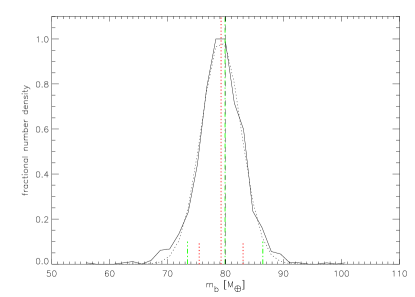
Figure 1: Distribution of derived mass of planet b (black solid line)derived using the partial data set. The Gauss fit to this distribution is shown as black dotted line. The best fit as well as the $1\sigma$ error range is indicated as red dotted line. The median of the distribution is indicated as black dashed line. The planetary mass and its uncertainty derived by H10 is indicated as green dashed-dotted line.

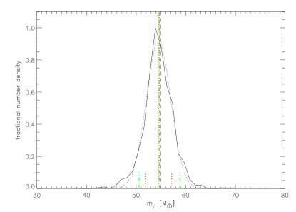
Figure 2: Distribution of derived mass of planet c (black solid line) derived using the partial data set. The Gauss fit to this distribution is shown as black dotted line. The best fit as well as the $1\sigma$ error range is indicated as red dotted line. The median of the distribution is indicated as black dashed line. The planetary mass and its uncertainty derived by H10 is indicated as green dashed-dotted line.

Figure 3: Radial velocity measurements from H10 compared to those predicted by our best fit for the partial data set. The time is given as BJD - 2454933.0.

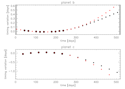
Figure 4: Transit timing variation measurement, i.e. the difference between the observed transit times and a linear ephemeris, of planet b (top) and planet c (bottom). Data by H10 (large circles) compared to our best fit (red squares) obtained using only these early TTV measurements. Error bars are smaller than the symbols. The small circles indicate the following transit times variations against the same linear ephemeris as later obsered by Kepler. The time is given as BJD - 2454933.0.

Figure 5: Deviation between the measured transit timing variations of planet b (top) and planet c (bottom) planet by H10 and our best fit. The time is given as BJD - 2454933.0.

Our best fit parameters for the partial data set are summarized in Table 2 and compared to pervious results. Our error bars are taken from the distribution of parameters as shown in Figures 1 and 2. The best fit model compared to the RV data is shown in Figs. 3. The comparison with Fig. (3) of H10 shows an nearly identical situation: The observed RV variations can be matched reasonably well, however, the deviation between the model and observation is up to 8 m/s and larger then expected given the error bars. Like in H10, we also conclude that more RV observations would be necessary to check for the influence of additional planets or stellar activity jitter. In Fig. 4 we show the TTV data together with our best fit of the partial data set and in Fig. 5 we show the residuals to that fit. The reduced $\chi^{2}$ of 2.4 is dominated by the deviations from the RV measurements while the TTV measurements can be matched within their error bars.

Basically, we can recover the literature values from H10 for the planetary masses and the mass ration which agree well within the error range. Also, the eccentricities and arguments of periastron agree within the error range. In the other orbital parameters, we find some discrepancies. We find a significantly lower orbital period for planet b but a higher for planet c.

The fit to the partial data is also extended towards later measurements (Fig. 4) and compared with the actual transits observed by Kepler. About 250 days after the last transit reported by H10 the deviation is already 0.1 days for planet b and 0.3 days for planet c. Given the small error bars, it is clear that the planetary parameters have to be re-determined using the full Kepler data set.

5 TTV analysis using the full data set

We repeated the analysis using the full data set in the same way as described in the previous section, except that we now allow for non coplanar orbits and increased the number of random starting values to 3000 (see Figures 6, and 7). The full data set also allows to constrain the planetary masses without including the RV data in the fit. As expected from the poor agreement between the extrapolated solution from the partial data set, the planetary parameters changed. The main change is a significant reduction of the planetary masses in our new fit, while the mass ratio agrees within the error range. In Table 3 we compare the new parameters to those we obtained from the partial data set (Table 2). The increase in the orbital period for planet b and the decrease for planet c are expected from the deviations seen in Figure 4.

Combining the fitted parameter $a/R_{\star}$ from Table 1 with the orbital semi major axis from the TTV fit (Table 3), we derive the stellar radius. Using this in combination with $r/R_{\star}$ (Table 1) provides the planetary radius, which then can be combined with the planetary masses (Table 3) to the mean planetary densities (Table 3, lower block).

Comparing the observed and calculated transit times in Fig. 8 now shows a good match over the whole observing period. This can also be seen from the residuals (Fig. 9) as well as from the reduced $\chi^{2}$ of 1.81. The lower planetary masses, however, lead to a less good match of the RV variations (Figures 10 and 11). We now have residuals of up to 12 m/s. Note, however, that the H10 masses were determined using the RVs in the fit, minimizing the RVs residuals by construction, whereas our full-dataset model did not fit for the RVs data.

Table 3: Fitted parameters (upper block) of the planetary system of Kepler-9 derived from the TTV analysis using the full Kepler data set. The osculating orbital elements are given at a reference time BJD=2454933.0. The stellar mass is an input parameter with a distribution according Havel et al. (2011), i.e. our errors take the uncertainties in the stellar mass into account. For comparison, we list our best fit parameters based on the TTV measurements from H10 (see Table 2). Note that those orbital elements are given at a reference time BJD=2454900.0. We also list derived quantities (lower block) for the stellar radius, the planetary masses, radii, orbital periods, and densities using the fitted parameters $a/R_{\star}$ and $r/R_{\star}$ from Table 1.

Parameter	this work		this work
	full data set		partial data set
	without RV		with RV
	best fit	$\sigma$	best fit	$\sigma$
m⋆ [M⊙]	1.05	0.03	1.05	0.03
mb/m⋆ [M⊕/M⊙]	43.0	0.7	75.4	3.3
mc/mb	0.6875	0.0003	0.69	0.004
Pb [days]	19.22418	0.00007	19.2159	0.0008
Pc [days]	39.03106	0.0002	39.084	0.003
eb	0.0626	0.001	0.10	0.02
ec	0.0684	0.0002	0.08	0.02
$i_{\rm b}$ [∘]	87.1	0.7	not fitted
$i_{\rm c}$ [∘]	87.2	0.7	not fitted
$\omega_{\rm b}$ [∘]	356.9	0.5	357.5	21.0
$\omega_{\rm c}$ [∘]	169.3	0.2	101.5	4.0
Mb [∘]	337.4	0.6	105.3	23.1
Mc [∘]	313.5	0.1	36.6	20.6
r⋆ [R⊙]	1.23	0.01
mb [M⊕]	45.1	1.5	79.6	3.6
mc [M⊕]	31.0	1.0	54.8	2.6
rb [R⊕]	11.1	0.1
rc[R⊕]	10.7	0.1
rd[R⊕]	2.0	0.02
ab [AU]	0.143	0.001	0.143	0.001
ac [AU]	0.229	0.002	0.229	0.002
ad [AU]	0.0271	0.0001
$\rho_{b}$ [g cm-3]	0.18	0.01
$\rho_{c}$[g cm-3]	0.14	0.01

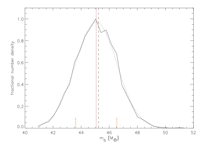
Figure 6: Distribution of derived mass of planet b using the full data set (black solid line). The Gauss fit to this distribution is shown as black dotted line. The best fit as well as the $1\sigma$ error range is indicated as red dotted line. The median of the distribution is indicated as black dashed line.

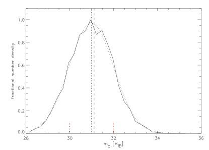
Figure 7: Distribution of derived mass of planet c using the full data set (black solid line). See also Fig.6.

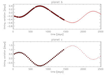
Figure 8: Transit timing variation measurement, i.e. the difference between the observed transit times and a linear ephemeris, of planet b (top) and planet c (bottom) planet (large circles) compared to our best fit (red squares) obtained using the full Kepler data set. The error bars are smaller than the size of the symbols. The small circles indicate the following transit times variations against the same linear ephemeris. The time is given as BJD - 2454933.0.

Figure 9: Deviation between the measured transit timing variations of planet b (top) and planet c (bottom) planet and our best fit using the full data set. The time is given as BJD - 2454933.0.

Figure 10: Radial velocity measurements from H10 compared to those predicted by our best fit using the full data set. We note that we do not include the RV data into our fit procedure but just derive it from the best fit model. The time is given as BJD - 2454933.0.

Figure 11: Residuals of radial velocity measurements from H10 compared to those predicted by our best fit using the full data set. The time is given as BJD - 2454933.0.

Table 4: Predicted future transit time for planet b and planet c from our best fit using the full data set. The time is given as BJD - 2454933.0

planet b
1468.30749	1853.21471	2238.70993	2623.31170
1487.53311	1872.48347	2257.96478	2642.53063
1506.76023	1891.76418	2277.21419	2661.74940
1525.98749	1911.03707	2296.46244	2680.96834
1545.21757	1930.32080	2315.70445	2700.18775
1564.44709	1949.59670	2334.94627	2719.40692
1583.68102	1968.88203	2354.18160	2738.62704
1602.91356	1988.15970	2373.41752	2757.84656
1622.15229	2007.44513	2392.64722	2777.06742
1641.38867	2026.72326	2411.87806	2796.28738
1660.63310	2046.00730	2431.10335	2815.50893
1679.87414	2065.28456	2450.33008	2834.72942
1699.12498	2084.56572	2469.55214	2853.95164
1718.37136	2103.84075	2488.77575	2873.17278
1737.62904	2123.11760	2507.99568	2892.39566
1756.88121	2142.38911	2527.21710	2911.61766
1776.14570	2161.66033	2546.43584	2930.84130
1795.40378	2180.92716	2565.65585	2950.06446
1814.67463	2200.19167	2584.87413	2969.28904
1833.93835	2219.45285	2604.09336	2988.51383
planet c
1477.96294	1867.51356	2255.75156	2646.06579
1517.01523	1906.32679	2294.69070	2685.14079
1556.05565	1945.12525	2333.66139	2724.21523
1595.07993	1983.91531	2372.66051	2763.28891
1634.08355	2022.70358	2411.68358	2802.36177
1673.06218	2061.49673	2450.72550	2841.43373
1712.01228	2100.30141	2489.78121	2880.50445
1750.93174	2139.12401	2528.84626	2919.57315
1789.82030	2177.97032	2567.91703	2958.63851
1828.67971	2216.84512	2606.99083	2997.69845

The discrepancy of the observed and calculated RV variations as well as possible slight systematic residuals in the TTVs of planet c raised the question whether or not we can find evidence for a forth, possibly non-transiting planet in the system. We therefore first searched for additional transiting planets in the system in the photometric model’s residuals using Optimal BLS (Ofir, 2014) but found none. We also repeated the dynamical analysis adding an outer, co-planer, plane to the system. Since the parameter range for an outer planet is huge, we restricted our search to orbits of the test planet in 3:2, 2:1, 5:2, and 3:1 mean motion resonances to planet c. No solution with a better reduced $\chi^{2}$ could be found. We note that the short time span of the RV data – less than one orbit of Kepler-9c – severly limit the orbits that one can hope to fit to such a test outer planet.

Additionally, we have also checked our assumption that planet d has no impact on our results: We included planet d in the dynamical model by fixing its orbital period at the measured value, assuming a co-planar and circular orbit, the latter motivated by the short circularization time scale at the small orbit distance, and determined the mean anomaly at the beginning of the integration to match the measured transit time $T_{mid,3}$. We then refitted the full TTV data set for planet d in the mass range of 1 to 30 Earth masses letting the parameters of planet b and c re-adjust. We find a very shallow $\chi^{2}$-minimum around 10,M_⊕ but with insignificant improvement compared to the tested mass range for planet d. The parameters of planet b and c are unaffected within their error bars. We conclude that we cannot derive any meaningful constraints on the mass of planet d and find our solution sumarized in Table 3 unaffected.

We conclude that neither an additonal outer planet in a low-order resonant orbit nor the inclusion of planet d can improve on the very systematic residuals of the RV signal. A more extended RV follow-up would be necessary in order to come to a more conclusive result.

6 Discussion and conclusion

6.1 Partial vs. full dataset

We re-analysed the Kepler-9 system using both the partial Kepler data set that was available to H10 and the full data set available today. The comparison between the previous and new results show, that a very good fit to a planetary system in first order mean motion resonance can be misleading if only a fraction of the interaction time scale is covered. Even the much longer currently available Kepler data set might not be sufficiently long for that. We therefore follow H10 and extrapolated our best fit model into the future (Fig. 8 and Table 4). Given the large TTVs, ground based observations even with a marginal detection of the transit should be able to check the solution proposed in this work.

H10 could confirm the Kepler-9b and Kepler-9c as planets from photometry alone, but could only place weak constraints on their masses without using RV data. They therefore included a few RV measurements in their fit, and it comes as no surprise that the RV fit is good since the partial photometry of the time did not have the constraining power to match the RV data. They also predicted that future Kepler data would be more constraining of the planetary masses, and indeed our results have smaller formal error bars on both planets’ masses from photometry alone. We note, however,that the systematic residuals shown in Fig. 9, and especially Fig. 11 cause us to warn of unmodeled phenomena, such as other planets in the system or longer time-scale interaction between the planets or stellar activity.

6.2 The revised planets

The scaled radii r${}_{b,c}/R_{*}$ we determined are slightly larger than the ones obtained by H10 by $\sim 3\sigma$ and $\sim 4.5\sigma$ for Kepler-9b and Kepler-9c, respectively. The new values are much more constrained with formal errors 5 to 8 times smaller. Actually, Kepler’s data allows in principle to determine the planets’ mass to $2.8\%$ and the planets’ radii to better than 0.2% – but those are limited by our knowledge of the host star properties. Furthermore, Kepler-9 was measured in short cadence mode (1 minute sampling instead of the regular 30-minute sampling) starting from Quarter 7, which allows for an even better timing precision (and thus mass determination). While we did not use short cadence data, using this data would have had little effect on the global uncertainty which is dominated by stellar parameters errors.

The newly determined masses and radii of Kepler-9b and -9c change the nature of these planets relative to the one described in H10. Both planets are now detetmined to have size similar to Jupiter’s but they are 7 to 10 times less massive than Jupiter, i.e. have densities about 1/3 of the density given in H10. Consequently, both planets have very low derived densities of $\rho_{b}\sim=0.18\,g\,cm^{-3}$ and $\rho_{c}\sim=0.14\,g\,cm^{-3}$ – among the lowest known. H10 specifically excluded coreless models for the planets, but the more abundant data we have today forces us to reconsider that Kepler-9b and -9c may not have cores at all. This result is of special interest in the context of the core accretion theory (Pollack et al., 1996): with masses of 30.6 and 44.5 $M_{\oplus}$ these planets have apparently just started their runaway growth when it stopped at this relatively rare intermediate mass.

Figure 12 shows the masses and radii of lower-mass ($M<100M_{\oplus}$) planets that have both mass and radius known to better than $3\,\sigma$ . It is evident that the new locations of Kepler-9b and -9c put them at the edge of the mass-radius distribution, with very low density and in a mass range that is very poorly sampled, and yet – both planets are now among the best-characterized exoplanets known with bulk densities known to $7\%$ or better. The recent successful launch of the GAIA mission further highlights that last point: the knowledge about both Kepler-9b and -9c in both radius and mass is limited by the knowledge about their host star. GAIA’s observations will fix Kepler-9’s properties to high precision, allowing to use other data (such as the available short cadence data) to further reduce the uncertainty on the physical parameters of Kepler-9b and -9c, and significantly so.

Finally, we note that Kepler-9d is now determined to have a radius of $2.00\pm 0.05R_{\oplus}$, an increase relative to H10. The increased size, together with the low metal content of its neighboring planets, suggest that Kepler-9d may not be rocky, or at least that it may have a significant volatiles fraction, again unlike the initial suggestion by H10. If this is true, then Kepler-9d is perhaps similar to the new and exciting subgroup of low-mass low-density planets (e.g. Kepler-87c or GJ 1214 Ofir et al., 2014; Charbonneau et al., 2009; Fortney et al., 2013)

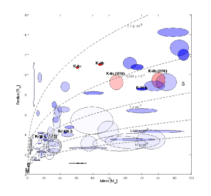
Figure 12: The mass-radius distribution of all well determined planets (both mass and radii determined to better than 3$\sigma$). For each planet the mass- and radius- semi-major axes represent the 1-$\sigma$ error bar, and the transparency is such that better determined planets are more opaque. Contours of constant bulk density are shown in dashed gray lines. The names of some of the better-determined planets are indicated. All planets are shown in shades of blue, but Kepler-9 which is shown in shades of red: larger (and more transparent) symbols for the H10 values, and smaller (and more opaque) symbols for the current study’s values. Solar system planets are shown as letters.

7 Acknowledgments

A.O. acknowledges financial support from the Deutsche Forschungsgemeinschaft under DFG GRK 1351/2.

References

- Agol et al. (2005) Agol, E., Steffen, J., Sari, R., & Clarkson, W. 2005, MNRAS, 359, 567
- Chambers (1999) Chambers, J. E. 1999, MNRAS, 304, 793
- Chambers & Migliorini (1997) Chambers, J. E. & Migliorini, F. 1997, in Bulletin of the American Astronomical Society, Vol. 29, AAS/Division for Planetary Sciences Meeting Abstracts #29, 1024
- Charbonneau et al. (2009) Charbonneau, D., Berta, Z. K., Irwin, J., et al. 2009, Nature, 462, 891
- Fortney et al. (2013) Fortney, J. J., Mordasini, C., Nettelmann, N., et al. 2013, ApJ, 775, 80
- Havel et al. (2011) Havel, M., Guillot, T., Valencia, D., & Crida, A. 2011, A&A, 531, A3
- Holman et al. (2010) Holman, M. J., Fabrycky, D. C., Ragozzine, D., et al. 2010, Science, 330, 51
- Holman & Murray (2005) Holman, M. J. & Murray, N. W. 2005, Science, 307, 1288
- Ofir (2014) Ofir, A. 2014, A&A, 561, A138
- Ofir et al. (2010) Ofir, A., Alonso, R., Bonomo, A. S., et al. 2010, MNRAS, 404, L99
- Ofir & Dreizler (2013) Ofir, A. & Dreizler, S. 2013, A&A, 555, A58
- Ofir et al. (2014) Ofir, A., Dreizler, S., Zechmeister, M., & Husser, T.-O. 2014, A&A, 561, A103
- Pollack et al. (1996) Pollack, J. B., Hubickyj, O., Bodenheimer, P., et al. 1996, Icarus, 124, 62
- Xie (2013) Xie, J.-W. 2013, ApJS, 208, 22