Validation of optimised population synthesis through mock spectra and Galactic globular clusters

Abstract

Optimised population synthesis provides an empirical method to extract the relative mix of stellar evolutionary stages and the distribution of atmospheric parameters within unresolved stellar systems, yet a robust validation of this method is still lacking. We here provide a calibration of population synthesis via non-linear bound-constrained optimisation of stellar populations based upon optical spectra of mock stellar systems and observed Galactic Globular Clusters (GGCs). The MILES stellar library is used as a basis for mock spectra as well as templates for the synthesis of deep GGC spectra from Schiavon et al. (2005). Optimised population synthesis applied to mock spectra recovers mean light-weighted stellar atmospheric parameters to within a mean uncertainty of 240 K, 0.04 dex, and 0.03 dex for $T_{\rm eff}$, $\log g$, and [Fe/H], respectively. We use additional information from HST/ACS deep colour-magnitude diagrams (CMDs) from Sarajedini et al. (2007) and literature metallicities to validate our optimisation results on GGCs. Decompositions of both mock and GGC spectra confirm the method’s ability to recover the expected mean light-weighted metallicity in dust-free conditions ($E(B-V)\lower 2.15277pt\hbox{$\;\buildrel<\over{\sim}\;$}0.15$) with uncertainties comparable to evolutionary population synthesis methods. Dustier conditions require either appropriate dust-modelling when fitting to the full spectrum, or fitting only to select spectral features. We derive light-weighted fractions of stellar evolutionary stages from our population synthesis fits to GGCs, yielding on average a combined $25\pm 6$ per cent from main sequence and turnoff dwarfs, $64\pm 7$ per cent from subgiant, red giant and asymptotic giant branch stars, and $15\pm 7$ per cent from horizontal branch stars and blue stragglers. Excellent agreement is found between these fractions and those estimated from deep HST/ACS CMDs. Overall, optimised population synthesis remains a powerful tool for understanding the stellar populations within the integrated light of galaxies and globular clusters.

1 INTRODUCTION

Fundamental information on the physical processes which dominate the formation and evolution of galaxies can be gleaned from the study of their stellar populations. Early studies of galaxies’ stellar content relied on the technique of population synthesis, wherein the integrated spectrum of a galaxy is decomposed into a sum of suitably-weighted spectra of individal stars with known basic properties such as temperature, surface gravity, and metallicity (Spinrad & Taylor 1971; Faber 1972; O’Connell 1976; Pickles 1985). In order to obtain information such as age or star formation history, stellar evolutionary models should then be applied subsequent to the decomposition. Advances in our knowledge of stellar evolution have however enabled a new technique for stellar population analyses, so-called evolutionary population synthesis (Renzini 1981; Buzzoni 1989; Bruzual & Charlot 1993; Maraston 1998). By combining individual stellar spectra with isochrones and an initial mass function, integrated spectra of entire galaxies (or stellar clusters) can then be constructed over a wide range of ages and metallicities. Thus, evolutionary population synthesis folds in evolutionary models as part of the spectral decomposition. The power of the latter technique to reduce the degrees of freedom in stellar population analyses resulted in the demise of the former.

However, various uncertainties affecting current stellar evolution models (e.g. thermally-pulsating asymptotic giant branch, horizontal branch, and blue straggler stars; Maraston 2007; Conroy et al. 2009), especially pertaining to the brightest phases of stellar evolution, are cause for concern in any application of evolutionary population synthesis. For instance, the presence of blue horizontal branch stars in elliptical galaxies, coupled to the lack of a predictive theory for their origins, can be misinterpreted as their having recently experienced a burst of star formation (Maraston & Thomas 2000). Population synthesis, on the other hand, should in principle be free from the outshining effect that uncertain phases of stellar evolution have on stellar population analyses. We therefore expect this technique to be able to unravel at once the contributions of all stars to the integrated light of a stellar system.

In light of these issues and the availability of exceptional computing power, we wish to re-examine and validate the population synthesis optimisation method as a means to provide estimates of the stellar content of unresolved systems independent of any assumed stellar evolution model. And while the latter is true, it should still be noted that the coverage in age, metallicity, and surface gravity of the adopted stellar basis may have a significant impact on the final spectral decompositions (Koleva et al. 2008).

Before applying the population synthesis technique to galaxy spectra, it must be rigorously tested on data samples for which the underlying stellar contents are known. In this paper, we use both mock and observational data to test the technique under realistic (imperfect) observing conditions. Owing to the existence of deep integrated spectra (Schiavon et al. 2005, hereafter S05) and colour-magnitude diagrams (hereafter CMDs; Sarajedini et al. 2007) as well as high-resolution star-by-star spectroscopic abundances (Harris 1996; Roediger et al. 2014, and references therein) for them, Galactic globular clusters (GGCs) provide the best astrophysical test bed for population synthesis.

Specifically, we test the ability of the technique to recover the luminosity-weighted distributions of stellar atmospheric parameters (effective temperature, surface gravity, metalliticy, and colour), as well as the contributions of various evolutionary phases to the integrated light of GGCs which can be directly validated with corresponding estimates based on CMDs. In doing so, we identify regions of parameter space (both observational and physical) where the technique may fail to reproduce known stellar system data. It should be noted that, without the inclusion of a stellar evolutionary model, population synthesis cannot derive evolutionary properties of stellar systems such as age and star formation histories; properties that we do not attempt to measure in this paper.

To our knowledge, no study of this kind has addressed the reliability of population synthesis methods using both mock and real data as constraints. Koleva et al. (2008) performed a similar study to our own using evolutionary population synthesis on the same S05 GGC spectra used here. We will show below that our population synthesis method is just as reliable in the determination of GGC metallicity despite the lack of stellar evolution modelling.

The computational engine central to our numerical decompositions is a non-linear bound-constrained optimisation. Similar spectral decompositions of stellar systems via constrained optimisation have been applied before (e.g. MacArthur et al. 2009; Cid Fernandes et al. 2005; Walcher et al. 2006). Other inversion methods used to fit stellar spectra or SSP models to integrated spectra have also been reported recently by, e.g. Vergely et al. (2002), Moultaka (2005), Ocvirk et al. (2006), Tojeiro et al. (2007), Koleva et al. (2008), and Koleva et al. (2009).

The organization of the paper is as follows. In Section 2, we present our libraries of GGC and stellar spectra. In Section 3, we describe the optimisation algorithm used for decomposing mock and observed integrated spectra into sums of individual stellar spectra, as well as establish the typical level of random and systematic errors inherent to any given decomposition. We then apply our algorithm in Section 4 to the GGC integrated spectra of S05 to determine the fractional contributions (by light) of stellar parameters (effective temperature, surface gravity and metallicity) for each cluster. These fractions in turn yield estimates of each cluster’s light-weighted metallicity and stellar evolutionary budget. Section 4.2 and Section 4.3 present a comparison against independent constraints. Our discussion and conclusions are presented in Section 5, followed by two appendices. Appendix A includes our reconstruction of each GGC spectrum analyzed in this paper. Finally, deep CMDs for the 24 S05 GGCs in common with the HST/ACS database of Sarajedini et al. (2007), along with their breakdown into the various stellar evolutionary zones, are presented and compared with CMDs derived from population synthesis in Appendix C.

2 SPECTRAL LIBRARIES

The GGC integrated spectra that we wish to model through population synthesis methods come from the S05 library. S05 obtained deep, drift-scan optical spectra of the cores of 41 GGCs using the R-C spectrograph on the Blanco 4-m telescope at the Cerro-Tololo-Interamerican Observatory. These data combine the merits of broad spectral coverage (${\sim}3350-6430$ Å), intermediate spectral resolution (FWHM ${\sim}3.1$ Å) and high signal-to-noise (50 $<$ S/N/Å $<$ 240 at 4000 Å). Further details on the observational setup or reduction methods for these spectra can be found in S05.

Population synthesis typically takes advantage of an extensive library of stellar spectra in order to reproduce the integrated spectrum of a (normally) unresolved stellar system. To reconstruct the S05 spectra, we use the Medium-resolution Isaac Newton Telescope stellar library (Sánchez-Blázquez et al. 2006; hereafter MILES), which consists of empirical spectra for 985 stars obtained at the 2.5-m Isaac Newton Telescope. The comparable wavelength range (${\sim}3525-7500$ Å) and resolution (FWHM=2.54 $\pm$ 0.08 Å; Cenarro et al. 2007; Falcón-Barroso et al. 2011) of these data and S05 makes the MILES library ideal for our purposes. Figure 1 shows sample spectra from both the S05 and MILES libraries, where the former (shown in blue) span the full metallicity range of the S05 library, while the latter (shown in red) span the full spectral range of the MILES library. A simple by-eye comparison of the continuum shapes from these two examples already suggests that GGC spectra are predominantly generated by cool (i.e., old) G-, K- and M-type stars rather than hot (i.e., young) O-, B- and A-type stars as expected given the mean age ($\lower 2.15277pt\hbox{$\;\buildrel>\over{\sim}\;$}10$ Gyr) of globular clusters. We will indeed confirm this impression in Section 4.1.

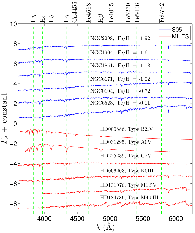
Figure 1: Representative spectra from the S05 and MILES spectral libraries, shown on an arbitrary flux scale. Vertical green dashed lines denote the locations of major (atomic) absorption features listed in Worthey et al. (1994), with the label of each feature provided at the figure top. The S05 and MILES spectra are stacked vertically in order of increasing metallicity ([Fe/H]) and effective temperature, respectively.

The successful decomposition of the GGC spectra hinges on the accurate characterization of both the wavelength calibration and spectral resolution of the S05 and MILES libraries. While the MILES spectra have a constant full width at half maximum resolution throughout their wavelength range (FWHM_M = 2.54 Å; Falcón-Barroso et al. 2011), that of the S05 spectra (FWHM_S) varies with wavelength according to,

$$\mathrm{FWHM_{\rm S}}(\lambda)=15.290-6.079\times 10^{-3}\lambda+9.472\times 10^{-7}\lambda^{2}-4.395\times 10^{-11}\lambda^{3}$$ (1)

where $\lambda$ is the wavelength in Å. This function gives FWHM${}_{\rm S}\simeq$ 3.1 Å at the central wavelengths (${\sim}4500-5500$ Å) of the S05 spectra and roughly 3.6 Å at their edges ($\sim$3350 Å and 6430 Å). The MILES spectra were therefore degraded by convolving with a Gaussian kernel to match the resolution of S05. A mean difference of 0.05 $\pm$ 0.13 Å between the centroids from S05 and MILES was measured, implying that the wavelength calibrations of the two libraries are consistent to within the random error, which is more than sufficient for our needs.

2.1 Stellar basis

We must now select a stellar spectral basis for our optimisation code. This basis would ideally comprise as many stellar types as possible whilst keeping the number of spectra manageable, lest our code be made computationally prohibitive. We first trimmed the original MILES library to exclude “exotic” stars (e.g. binaries, emission line objects), highly reddened stars (with $E(B-V)>0.1$), stars exhibiting spectral peculiarities, and stars with unknown distance measurements. Stars belonging to globular clusters were also removed to avoid possible contamination in their spectra and because their metallicities are assigned the mean of the entire globular cluster. All remaining stars were manually inspected for emission lines and other possible spectral blemishes. In the end, we were left with a “restricted” library of 774 stars from which to construct our stellar basis.

The range of physical parameters spanned by the stars in the restricted MILES library is highlighted in Figure 2. For each MILES star, the atmospheric parameters $T_{\rm eff}$, $\log g$ and [Fe/H] were extracted from Prugniel et al. (2011), where $T_{\rm eff}$ is the effective temperature (in K), log$(g)$ is the surface gravity (in cgs units), and [Fe/H] is the metallicity.

Each star in the full MILES library is shown as a grey dot while the restricted set is shown as blue dots in the top row of Figure 2. The group of stars in the middle panel at [Fe/H]$=-0.84$ are all members of the globular cluster NGC 6838 and are thus ignored. Many of the high $T_{\rm eff}$- low $\log g$ stars were also removed in light of strong emission lines in their spectra.

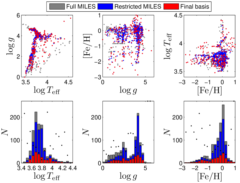
Figure 2: (Top panels) Bivariate distributions of the atmospheric parameters $T_{\rm eff}$, $\log g$ and [Fe/H] for the full MILES library, as well as two of its subsets (see Section 2.1 for details). (Bottom panels) Distribution of each atmospheric parameter in the full MILES library and its two subsets. Black points above each bin indicate the coverage of the final basis relative to the full MILES library, scaled from 0 to 1 in each panel from bottom to top respectively.

To minimize degeneracies and safeguard against computationally expensive optimisations, a subset of our restricted stars was chosen such that each member had to be above a minimum distance from all others in the 3-dimensional parameter space of $T_{\rm eff}$, $\log g$ and [Fe/H]. To ensure that each parameter was sufficiently sampled, a minimum (arbitrary) distance of 1/17th of the size of the parameter space was chosen. That distance corresponds to 0.07, 0.35, and 0.24 in $\log$ $T_{\rm eff}$, $\log g$ and [Fe/H] respectively. The fact that this spacing is larger than the typical errors in these parameters prevents degeneracies in our basis. We have verified that choosing a smaller distance (and thus a larger basis) does not affect our results. Our final stellar basis of 242 stars, hereafter “final basis”, is shown with red points in Figure 2. Fine sampling of the final basis is shown with histograms in the bottom panels of Figure 2, following the same colour scheme as its top panels. A black dot also indicates the fraction of MILES stars used for the final basis in each bin. The final basis includes stars which nicely sample the parameter space defined by the entire MILES library. Because the distributions are not uniform, any random error in our derived atmospheric parameters will likely bias the results toward the medians of these distributions.

3 Optimisation Method

3.1 The Algorithm

To disentangle the light-weighted stellar populations that make up the integrated spectra of GGCs, we set up an optimisation method in MATLAB which follows closely that presented in MacArthur et al. (2009). The overall optimisation problem can be summarized as trying to find the global minimum of a merit function $f(\vec{x})$ subject to linear constraints $a<x_{i}<b$. The merit function to be minimized is defined as,

$$\mathrm{Merit}=\left({\frac{1}{N-M}\sum\limits^{N}_{i=1}R_{i}^{2}}\right)^{\frac{1}{2}},$$ (2)

where $N$ is the number of data points included in the fit, $M$ is the number of stellar templates in the basis, and

$$R_{i}=w_{i}(G_{i}-S_{i}),$$ (3)

where $G_{i}$ is the flux of the S05 GGC spectrum at wavelength $\lambda_{i}$, $w_{i}$ is the weight of the $i^{th}$ pixel, and $S_{i}$ is the modelled GGC flux at $\lambda_{i}$ given by,

$$S_{i}=\sum\limits^{M}_{j=1}x_{j}F_{ji}.$$ (4)

Here $F_{ji}$ denotes the flux at the $i^{th}$ wavelength of the $j^{th}$ template, and $x_{j}$ is the relative contribution of the $j^{th}$ template to the synthesized spectrum. We define the weights per pixel $w_{i}=m_{i}\sigma_{i}^{-2}$, where $\sigma_{i}$ is the error on $G_{i}$ and $m_{i}$ can take a value of 0 or 1 to mask out blemishes in the GGC spectra (see S05). We take $\sigma_{i}^{2}$ as the variance given by the ratio of the SED to its S/N spectrum.

No templates can acquire a negative contribution to the synthesized spectrum as this would be unphysical. That is,

$$x_{j}\geq 0,~{}~{}~{}\forall~{}j=1..M$$ (5)

As in MacArthur et al. (2009), we have used the L-BFGS-B optimisation algorithm to minimize the merit function. This algorithm is a limited-memory quasi-Newton code designed for the problem of bound-constrained optimisation. The advantage of L-BFGS-B is that it does not require the full Hessian matrix at each iteration, but rather uses an approximation based on earlier iterations. This approximation is very useful in problems like ours wherein hundreds of independent variables may exist and computing the full Hessian can be computationally expensive and unnecessary. A MATLAB implementation of L-BFGS-B was obtained from http://www.cs.ubc.ca/ pcarbo/lbfgsb-for-matlab.html.

We also compare in the next section a similar optimisation routine, called fmincon, which is inherent to the MATLAB package. The latter uses an “interior-point” optimisation method. It will be shown below to perform poorly relative to L-BFGS-B in the case of realistic (noisy) data.

3.2 Tests with Mock Spectra

We must first test the internal accuracy of L-BFGS-B and fmincon in the context of our optimisation problem. To do so, mock composite spectra are created by summing individual stellar spectra from our final basis which can then be applied to either code. More specifically, a mock spectrum is created by first selecting ten stars from the final basis at random and giving them randomly-assigned positive weights $p_{i}$, subject to the constraint $\sum\limits^{10}_{i=1}p_{i}=1$ with each $p_{i}>0.05$; all other stars in the basis were given $p_{i}=0$. The basis spectra are then multiplied by their $p_{i}$ and summed to produce the mock spectrum. The figure of merit of our test is its ability to recover the correct $p_{i}$ for all of the stars in our final basis at once (including those with $p_{i}=0$).

In order to simulate realistic conditions, Gaussian noise is added to the spectrum up to a desired $S/N$ ratio per pixel. The two optimisation codes can then be tested with the same mock spectra in order to compare the recovered $p_{i}$. A given optimisation is run ten times for each $S/N$ ratio, varying the set of ten stars in the mock spectrum and their $p_{i}$ each time. The $S/N$ is varied over the range [10,10000] and the case of no additional noise is also considered. Such a large range is considered to show the very slow convergence of FMINCON with increasing $S/N$.

Initial conditions are required for these optimisation routines. By fitting to the same mock spectrum repeatedly with different initial conditions each time, we find that the optimisation results are largely insensitive to the initial conditions. Therefore for this and all subsequent decompositions, we use equal weights for all the basis stars as initial conditions for the optimisation code.

For each $S/N$ value, the relative residuals between the ten non-zero ($p_{i}\neq 0$) mock spectrum weights and their corresponding fit weights are computed and averaged over the ten weights and ten tests. These averaged relative residuals are shown as a function of $S/N$ in Figure 3. When no noise is added to the artificial spectrum, fmincon and L-BFGS-B both converge to within $0.1$ per cent of the correct result. However, in the presence of noise, L-BFGS-B proved far more reliable and converged faster. In light of these results, we only use L-BFGS-B for subsequent optimisations. Since the S05 spectra have $S/N$ levels in the range [50,240], Figure 3 shows that relative errors of $\sim$20 per cent should be assigned to our derived light-weighted fractions of individual stars. However, this error may likely result from degeneracies in our final basis. We show later in this section that the error in the recovered atmospheric parameters is much smaller than 20 per cent.

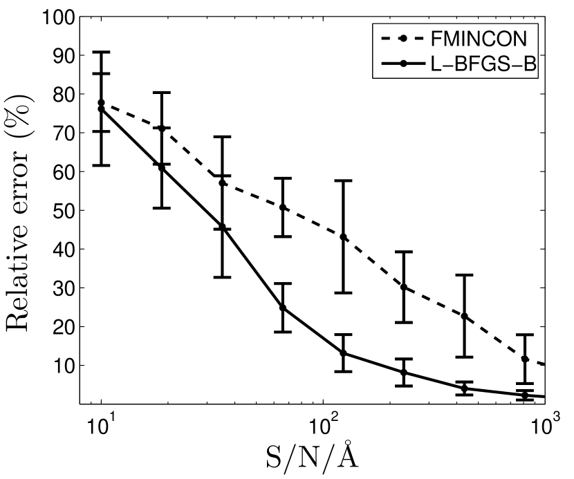
Figure 3: Relative error between the recovered and assigned weights in the decompositions of mock spectra as a function of $S/N$. Error bars represent the rms spread from ten realisations of the spectra at each $S/N$ value. The dashed and solid lines correspond to the two optimisation algorithms described in the text (see legend). The relative error at each $S/N$ value corresponds to the absolute difference between the fit and expected weights, divided by the expected weights and averaged over ten trials.

In assessing the internal errors of our optimisation procedure, false positives may also contribute to the random noise involved in the decomposition results. We test for this by computing for each run the maximum fractional contribution (by light) of those stars whose weights are assigned to be zero in the mock spectra. This maximum deviation from zero is averaged over all tests and is shown as a function of $S/N$ in Figure 4. Considering again the $S/N$ range of the S05 spectra, we infer that the random noise level for all subsequent fits should be less than 5 per cent. Therefore, any fractional contributions above 10 per cent will be significantly different from random noise at the 2$\sigma$ level.

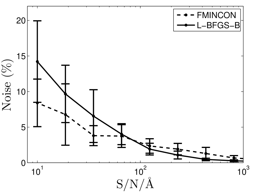
Figure 4: As in Figure 3 but here showing the maximum noise level in the mock spectra decompositions. The noise at each $S/N$ per Å was computed by taking the maximum fit weight expected to be zero in each trial run and averaging over all 10 trials for that $S/N$ ratio.

A similar test to the one above uses mock spectra constructed instead with stars external to the final basis but included in our restricted MILES subsample (see Section 2.1). The final basis is thus fully independent from these mock spectra. We run our code on five different mock spectra constructed this way. No noise is added here since the noise intrinsic to the spectra is now independent between these two datasets.

Since the assigned and recovered weights for stars cannot be directly compared in these tests (the parent samples are different), we evaluate the performance of the L-BFGS-B routine through cumulative distribution functions (CDFs) of the resulting luminosity fractions which comprise the mock and fitted spectra, as a function of their atmospheric parameters. The CDFs are shown in Figure 5 where the assigned and fitted weights are represented by the blue and red curves, respectively. For reference, the CDFs obtained if all of the final basis stars are given equal weights (initial conditions of the optimisation routine) are shown as green curves. The overall qualitative impression from Figure 5, with the red and blue CDFs being very similar, is that L-BFGS-B is quite robust at recovering the right mix of stellar parameters for the mock spectra. Mean light-weighted atmospheric parameters were computed for each test and compared between assigned and recovered spectra. These means can be seen in blue and red text in each panel respectively. The mock and recovered values agree within the uncertainties, which are computed from the error in the atmospheric parameters from Prugniel et al. (2011) in addition to an assumed error of 20 per cent in each derived light-weighted fraction. The mean residuals between assigned and recovered parameters are 240 K, 0.04 dex, and 0.03 dex for $T_{\rm eff}$, $\log g$, and [Fe/H], respectively. Thus, under these ideal (mock) conditions, population synthesis is excellent at recovering atmospheric parameters from integrated spectra.

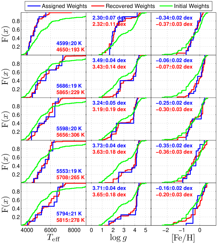
Figure 5: Comparison of the cumulative distribution functions (CDFs) in the space of the stellar parameters $T_{\rm eff}$, $\log g$, and [Fe/H] obtained from decompositions of mock spectra constructed from the MILES database but external to our final basis. The blue CDFs correspond to the mock spectra parameters derived from randomly assigned weights; the red CDFs are based on parameters recovered by our L-BFGS-B optimisation code. The green histograms represent the initial conditions for the optimisation program (i.e., all stars given equal weighting). Each row corresponds to a different mock spectrum, while each column represents a different atmospheric parameter. The light-weighted mean atmospheric parameters for mock and fit spectra are also shown in blue and red text respectively.

Since our analysis depends on matching the full SED of a stellar system, and not strictly on line indices, a blue-ward depression of the continuum due to dust extinction would clearly affect our ability to recover the right stellar mix. Line indices are indeed largely impervious to dust extinction effects (MacArthur 2005) but the latter is not true for full SED fitting. In order to quantify the influence of dust reddening on our spectral optimisations, mock spectra created from stars external to the main spectral basis were reddened according to the Milky Way extinction law (Cardelli et al. 1989).

The optimisation is performed on both reddened and non-reddened mock spectra through ten random realisations. Figure 6 shows the fit to a sample mock spectrum before and after reddening. In all cases, results were the same: fits to the non-reddened spectra are excellent, but application of a reddening law with $E(B-V)=0.35$ to the mock spectrum prior to optimisation causes a poorer fit. The highest discrepancies arise at prominent absorption features such as Mg₂, Fe5250, and H$\beta$ whose strengths depend strongly on metallicity and age.

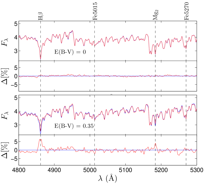
Figure 6: Fits to mock spectra before and after reddening (top and bottom sets of panels, respectively). The mock and fit spectra are shown in blue and red, respectively. Residuals are shown below the spectra. The mock spectrum in the bottom panel was reddened with $E(B-V)=0.35$. Important spectral features are indicated above the plot.

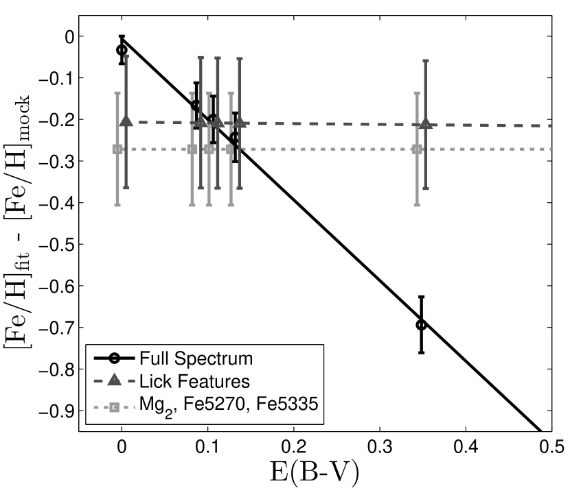
Figure 7: Residuals between the light-weighted metallicities of mock spectra ([Fe/H]_mock) and those of our population synthesis fits ([Fe/H]_fit) as a function of reddening applied to the mock spectra prior to fitting. Fits to the full spectrum, Lick features only, and only three metallicity-sensitive features are shown as circles, triangles, and squares respectively. Error bars indicate the rms dispersion over 10 tests. Linear fits to the data are also shown with different line types (see legend). For clarity, the data points for the fits to Lick or metallic features are offset in $E(B-V)$ by $\pm 0.005$ respectively.

To investigate the effect of reddening on the recovered metallicity, we compute a light-weighted metallicity of the mock and fit spectra, and average the difference over the ten realisations. This process is repeated with a range of reddening values. In Figure 7, we show the metallicity residuals between the fit and mock spectra as a function of applied reddening with circular points. Error bars indicate the rms dispersion over all ten realisations. When no reddening is applied, we recover the original metallicity accurately, with a mean $\Delta$[Fe/H]$=-0.018\pm 0.023$. When the mock spectra are reddened, we recover a lower than expected metallicity, an effect which grows linearly with $E(B-V)$.

In order to control this trend, we attempt to remove the effect of reddening from the reddened mock spectra by subtracting their continua. This procedure is performed by fitting and dividing by linear pseudo-continua around 13 prominent absorption features (hereafter “Lick features”) as in Worthey et al. (1994). The continuum level defined by the spectral region outside each feature is set to zero, leaving us with only 453 non-zero pixels per spectrum compared with 2770 in the full-spectrum case. We remove the continua this way for both the reddened and non-reddened MILES spectra (including the basis) and rerun the decompositions. Results of this test are shown as triangular points in Figure 7. With reddening effects removed from the spectra, we measure [Fe/H] consistently to within an error of 0.4 dex. Above $E(B-V)=0.15$, the derived metallicities are consistently better than when fitting to the (reddened) full spectrum indicating that this dereddening task was successful. However, for weakly reddened spectra, the fit to the full spectrum results in a more accurate value of [Fe/H]. In the weakly-reddened regime, one thus ought to fit to as many pixels as possible in order to maximize the accuracy of the derived parameters in a stellar population.

Note that the derived [Fe/H] values in this test tend to be underestimated. Since the metallicities of these mock spectra are generally higher (-0.5 $\leq$ [Fe/H] $\leq$ 0) than the mean metallicity of the basis ([Fe/H] $\sim-0.5$), random errors are expected to on average bias the average to underestimate the metallicities of these mock spectra, as observed. Indeed, we have checked that forcing the mock spectra to have [Fe/H] $<-1$ yields an overestimate in metallicity of 0.1 to 0.2 dex for highly reddened mock spectra.

In an attempt to increase our metallicity sensitivity, an additional test was performed where we instead fit only to three metallicity-sensitive spectral features: Mg₂, Fe5270, and Fe5335. Results of this test are shown as square points in Figure 7. Again, no trend with reddening is observed. However, the error in [Fe/H] estimates is now larger due to the even lower number (122) of pixels remaining in the spectra.

Our tests confirm both the code’s ability to recover the correct metallicity in dust-free conditions and to fail in the presence of dust. Full-spectrum population synthesis of integrated stellar spectra thus ill-advised for highly-reddened (e.g. low latitude) stellar systems without appropriate dust modelling.

4 Population Synthesis of Galactic Globular Clusters

4.1 Population Synthesis of the S05 GGC Spectra

The L-BFGS-B optimisation code was applied to the S05 GGC spectra using our final basis of 242 stars. Because the stars in the final basis are sampled mostly from the solar neighbourhood, and thus have similar alpha abundance patterns to the GGCs, we do not expect alpha-enhancement to be a concern (see Schiavon 2007). As in Section 3.2, we have also verified that our results are insensitive to initial conditions when fitting to GGC data. Therefore we use equal weighting for each basis spectrum as initial conditions.

In light of our tests in Section 3.2 and the fact that many of our GGC spectra suffer from Galactic extinction, we have implemented a reddening correction in Equation (3) by multiplying $S_{i}$ by a Cardelli reddening law of the form $e^{-\tau(\lambda)}$, where:

$$\tau(\lambda)=R_{V}E(B-V)\left(a(x)+\frac{b(x)}{R_{V}}\right)\frac{1}{1.086}.$$ (6)

and $a(x)$ and $b(x)$ are defined in Cardelli et al. (1989). We adopt $R_{V}=3.1$ for the Milky Way. For each GGC, we varied $E(B-V)$ in Equation (6) in steps of 0.02 from 0 to 1. The fit with the lowest value of the Merit function qualified as our best.

Comparisons of the synthesized and original spectra, along with the residuals of the fit, are shown in the electronic version of Appendix A for all 41 GGCs. The residuals were computed by taking the difference between the fitted and original spectra and normalizing by the mean value of the latter. $\chi^{2}$/dof values (hereafter $\chi^{2}$) are also shown for each decomposition. As in MacArthur et al. (2009), these values are computed as the ratio between the actual and expected variance in the fit. Most of our fits are excellent, such as those of NGC 1851 and NGC 1904 with $\chi^{2}\sim 1$, and demonstrate the applicability of our method.

The luminosity fractions of different stellar types which make up the total light of our GGCs, as inferred from our optimisation code, are binned by $T_{\rm eff}$, $\log g$, and [Fe/H] and plotted in Figure 8. Each colour bar in this figure represents the fit to a different cluster, ordered by metallicity. Recall that the relative uncertainty assigned to the weight of a given star is $\sim$20 per cent and that the absolute noise level is $\sim$5 per cent (see Section 3.2). However in this figure, the mean error in the magnitude of each colour bar will be less than that for individual stars. As a conservative upper limit, we still assign these same 20 per cent errors to the colour bars in this figure. Therefore all light fractions in this figure contributing less than 5 per cent may be considered noise.

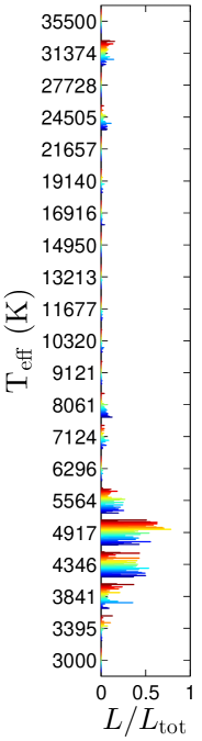
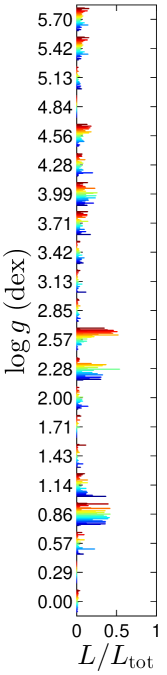
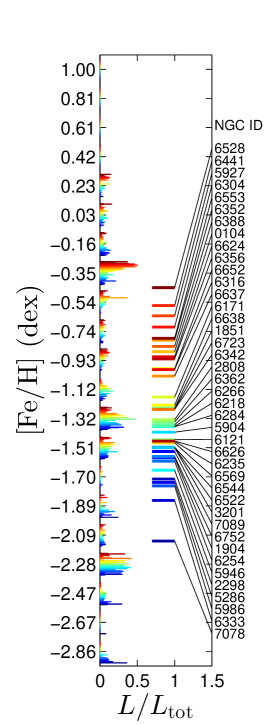
Figure 8: Optimised fractional contributions of final basis stars to each of the 41 S05 GGC spectra versus total cluster $V-$band luminosity, binned by either $T_{\rm eff}$, $\log g$  or [Fe/H]. Each colour strip represents the best final fit of a separate GGC, organized from low (bluer) to high (redder) metallicity. The values on the Y-axis correspond to the lower bounds of each atmospheric parameter bin. The derived light-weighted metallicity of each cluster is also indicated on the right side of the right panel, with a black line connecting each NGC ID with its metallicity.

In the $T_{\rm eff}$ regime, most of the contribution ($\sim$90 per cent) to the total light of the GGCs comes from stars with $T_{\rm eff}$$\sim$4000-6000 K. Interestingly, two very hot stars ($2.4$ and $3.1\times 10^{4}$ K) together make a small $\sim$5 per cent contribution to all the fits.

The fact that our modelling of these old systems requires very hot blue stars in all cases is certainly odd, and for some it might be a numerical artifact. This is especially true for GGCs such as 47 Tuc and NGC 6652 which are not expected to harbour such hot stars. Not surprisingly, the contribution from these hot stars in these clusters is less than our expected 5 per cent random error. Thus we may be overfitting these spectra in an effort to numerically minimise the residuals. However, in the cases where the hot star contribution does exceed 5 per cent, the decomposition would then be physically motivated; that is, these clusters are known to have a significant population of hot (e.g. blue horizontal branch and blue straggler) stars. Such is the case for e.g. NGC 6752 and 7089 (see Table 1 and Appendix C).

We find that these hot stars are necessary in order to obtain an accurate fit to the integrated spectra. Indeed, setting their light-weighting to zero after the optimisation yields a poor fit. The need for hot stars in similar fits was also reported by Koleva et al. (2008) who found that adding a contribution of very hot stars ($T_{\rm eff}$ = 6000 to 20 000 K) to their fits to the S05 spectra improved the match considerably, especially for clusters with strong blue horizontal branches.

The largest mean contributions to the total light in the $\log g$ regime come from high surface gravity main sequence stars ($\sim 35$ per cent between $\log g$ = 3.42 and 4.84 dex) and low surface gravity red giant stars ($\sim 33$ per cent between $\log g$ = 0.5 and 1.43 dex). A slightly smaller contribution of $\sim 28$ per cent on average comes from intermediate surface gravity stars with $\log g$ between 2.28 and 2.85 dex.

In the [Fe/H] regime, contributions come from a wide range of values. For clarity, the mean light-weighted metallicity of each GGC is indicated on the right side of the right panel. GGCs with low (high) metallicity have larger contributions from low (high) metallicity stars, as expected. Section 4.2 provides a more detailed comparison between these derived metallicities and current literature estimates.

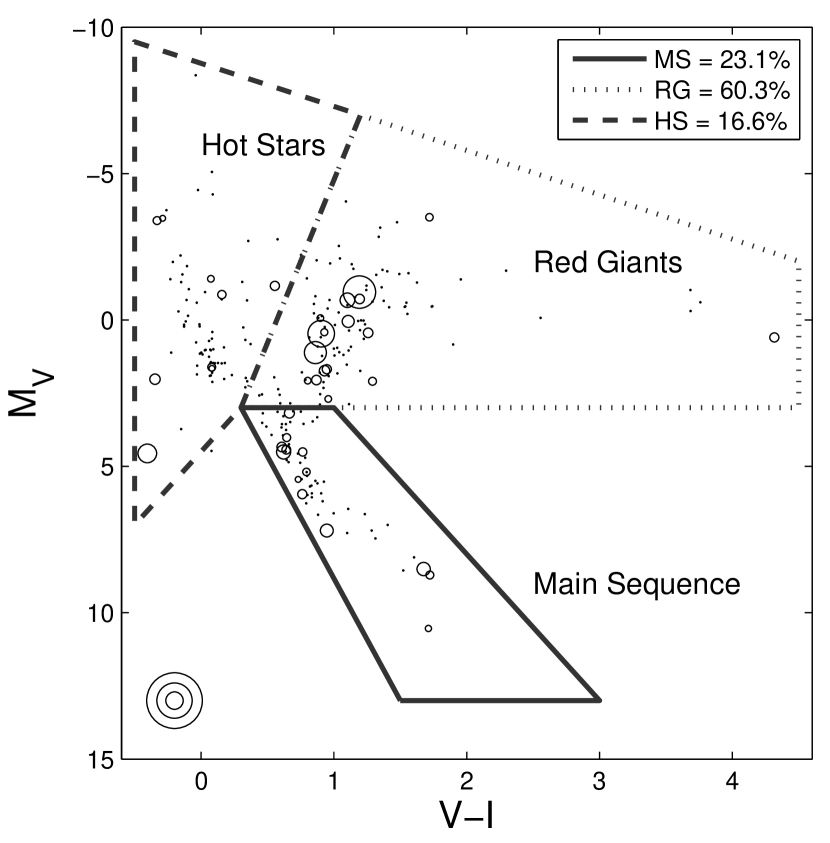
Figure 9: Mean fractional contributions (by light) of MILES stars to the spectra of all 41 GGCs plotted on a colour magnitude diagram, as indicated by the area covered by each point. Concentric circles at the bottom left corner indicate contributions of 5 per cent, 20 per cent, and 50 per cent. The legend indicates the total contribution from hot stars (HS), main sequence (MS), and red giant branch (RG) stars.

For a better visualisation of these results, Figure 9 shows the fractional contributions by light of MILES stars to the GGC spectra, averaged over all 41 fits to our GGCs. Relative contributions are directly proportional to the area of each circle. For reference, concentric circles are drawn in the bottom left corner to indicate contributions of 5 per cent, 20 per cent, and 50 per cent respectively. Rough stellar evolutionary zones have been sketched to investigate the contribution of various phases of stellar evolution. Because of the coarse resolution of the MILES library in (V-I) - $M_{V}$ space, only three zones have been drawn: Lower main sequence (MS), red giant branch (RG), and hot stars (HS). We find that roughly 60, 23, and 17 per cent of the integrated light of GGCs comes from each zone, respectively. As we shall see in Section 4.3, these evolutionary phase fractions agree well with the stellar fractions inferred from GGC CMDs, thus lending our optimisation method further support.

4.2 Metallicity Comparisons

We can also test our code’s ability to reproduce known GGC metallicities. Figure 10 compares literature values of [Fe/H] with those obtained through our decompositions. The error bar in the top-left panel represents the nominal uncertainty in the fitted values, based on our mock spectra decompositions (see Section 3.2).

The top-left panel of Figure 10 shows a comparison between the metallicities from Harris (1996, circa 2010) and fits to our GGCs. The mean and rms offset between our fits and literature values ($\Delta$[Fe/H]) are indicated in each panel. Between [Fe/H] of -1.5 and -1, the two datasets are in remarkable agreement. However, we tend to underestimate and overestimate [Fe/H] at higher and lower metallicity, respectively.

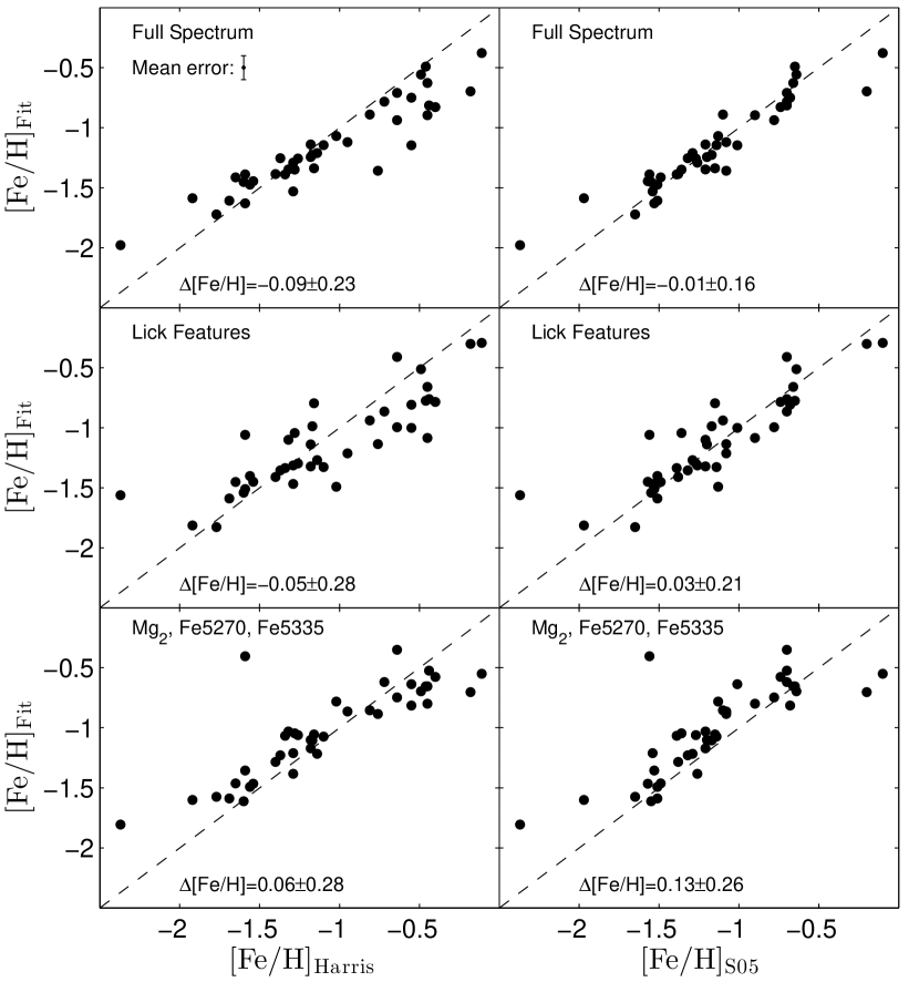
Figure 10: Comparison between metallicities derived from our optimisation synthesis of S05 GGC spectra and those from the Harris (1996) catalogue (left column) or S05 (right column). 1:1 relations are shown as dashed lines. The top row shows results from population synthesis using the full spectrum. The middle and bottom panels show the results of fitting only continuum-subtracted Lick features (thirteen generally prominent and three metallicity-sensitive features, respectively). Mean and rms metallicity offsets are indicated in each panel.

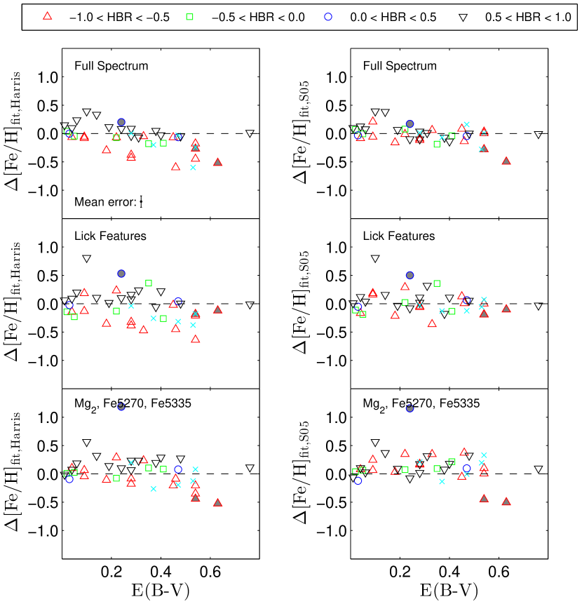
Figure 11: Residuals between metallicities derived from our optimisation synthesis of S05 GGC spectra and metallicities taken from the Harris (1996) catalogue, as a function of $E(B-V)$ (also taken from Harris 1996). Poor fits ($\chi^{2}>5$) are indicated with gray-filled markers. Points are styled according to horizontal branch ratio (HBR; see legend), while clusters without an HBR estimate are shown as cyan x’s.

This discrepancy at high metallicity may stem from the fact that metal-rich GGCs are mostly located near the Milky Way mid-plane and suffer more extinction than those lying above it. The top-left panel of Figure 11 shows the difference between our inferred (light-weighted) mean metallicity values and those taken from the 2010 edition of the Harris (1996) catalogue, as a function of colour excess $E(B-V)$. Here, poor fits ($\chi^{2}>5$) are indicated with filled gray markers. Data points are also coloured according to horizontal branch ratio (HBR), defined as HBR = (B-R)/(B+V+R), where B, V, and R are the number of stars bluer than, within, and redder than, the RR lyrae region of an HR diagram, respectively (Harris 1996). Thus a low HBR indicates a higher fraction of red-to-blue stars. For GGCs with low (negative) HBR and high reddening ($E(B-V)>0.15$), we underestimate [Fe/H] relative to the Harris (1996) values. This trend corroborates our results of mock tests with reddening in Section 3.2. In this first pass, it would appear that our Cardelli reddening correction was unsuccessful; however, we show below that this is not the case.

Cezario et al. (2013) also estimate [Fe/H] for the S05 GGCs via spectrum synthesis with the modelling program ULySS using for a basis SSP models based on MILES rather than the (empirical) MILES itself. When comparing with the [Fe/H] values of Carretta et al. (2009), they achieve $\Delta$[Fe/H] =$-0.15\pm 0.17$. Note that comparing with Carretta et al. (2009) instead of Harris (1996) does not change our results, which is expected since the Harris catalogue is largely based on that of Carretta et al. (2009). Thus, relative to Cezario et al. (2013), our method yields a smaller net offset but similar scatter with $\Delta$[Fe/H] =$-0.09\pm 0.23$.

In order to investigate and ultimately remove any reddening dependence, we subtract the continua of both the GGC and template MILES spectra using the same method as in Section 3.2, and rerun the decompositions. Note that this time we do not include the Cardelli reddening law coefficient as in fits with the full spectrum. The middle rows of Figures 10 and 11 show the result of this exercise. The left middle panel of Figure 10 indicates that the discrepancy between [Fe/H] derived from our decompositions and Harris (1996) for highly reddened GGCs is largely unchanged, and now exhibits more scatter.

Despite our continuum subtraction, the trend with reddening is still observed. Furthermore, we still find a lower than expected [Fe/H] for GGCs with negative HBR, but satisfactory agreement for those with positive HBR. This discrepancy may be partially explained by the fact that the 2010 version of the Harris (1996) catalogue uses a different metallicity scale than does Prugniel et al. (2011) for the MILES stars. The Harris (1996) values have been converted to a new scale defined by Carretta et al. (2009), while Prugniel’s scale agrees with that used by Sánchez-Blázquez et al. (2006), whom in turn used Soubiran et al. (1998) as a reference for their [Fe/H] values. Thus, rather than using the current Harris (1996) catalogue, we compare our derived [Fe/H] values with those compiled (and derived) by S05. Their [Fe/H] values are taken from Kraft & Ivans (2003) or Carretta & Gratton (1997), or extracted using their own spectroscopic methods.

The right-hand column of Figure 10 shows a comparison between the [Fe/H] values derived from our decompositions and those reported by S05. The top-right panel of this figure shows that our values for clusters with high [Fe/H] are in much better agreement with S05 than with Harris (1996, 2010 version), even when fitting to the full spectrum. Cezario et al. (2013) also find better agreement when comparing with S05 values ($\Delta[{\rm Fe/H}]=-0.05\pm 0.16$), whereas we find $\Delta[{\rm Fe/H}]=-0.01\pm 0.16$. Thus our errors in [Fe/H] are likely not driven by our inability to measure [Fe/H], but rather due to systematic uncertainties in the reference library.

Our scatter is consistent with a similar study by Koleva et al. (2008), who performed population synthesis on the S05 GGC spectra using single stellar population models based on the MILES library. They report a standard deviation of 0.17 dex between their determined [Fe/H] and those from S05. It is remarkable that we can achieve a similar result using only stellar spectra from MILES as a basis, without any evolutionary modelling.

Despite our corrections, we still seem to overestimate [Fe/H] at the low metallicity end ([Fe/H] $<-2$) when comparing to S05. This discrepancy might be due to incompleteness in our basis for stars with [Fe/H] $<2$, as is shown in the right-hand column of Figure 2. In an attempt to correct for this, we allow all MILES stars with [Fe/H] $<2$ into our basis regardless of peculiarities, and rerun the decompositions but no improvement is found. This is not surprising since the entire MILES library itself contains few stars below this metallicity.

For completeness we show the result of fitting to only the Lick features in the middle-right panel (again without a Cardelli reddening correction). While no trend with reddening is observed, the scatter is much higher than when fitting to the full spectrum. The same panel in Figure 11 shows that the residual trend with $E(B-V)$ has disappeared and shows lower scatter than when comparing with Harris (1996) [Fe/H] values, indicating that this task was indeed successful.

Rather than using all of the prominent features in our continuum-subtracted spectra, we now attempt to further improve the recovered metallicities by considering only three of the most metallicity-sensitive lines: Mg₂, Fe5250, and Fe5335. These results are displayed in the bottom panels of Figures 10 and 11. In this case comparisons between our fit [Fe/H] and those of Harris (1996) and S05 show good agreement. This method however overestimates metallicities for most of the GGCs regardless of our choice of [Fe/H] library comparison. This is likely because we err toward the mean of the distribution of atmospheric parameters in the basis ([Fe/H] $=-0.5$; see Section 3.2) which is higher than the [Fe/H] of most of our GGCs. Indeed, for [Fe/H] $>-0.5$, we tend to underestimate [Fe/H] when comparing with Harris (1996) values, a phenomenon consistent with our tests with mock spectra.

We thus conclude that, in terms of measuring light-weighted metallicities of highly reddened stellar systems accurately, fitting to the full spectrum with the inclusion of an appropriate reddening law yields the best results. However, in the absence of a reliable reddening correction, fitting to many spectral features with the continuum subtracted is a viable alternative. In the absence of significant reddening, fitting to the full spectrum yields the most accurate and precise metallicities.

4.3 GGC Population Synthesis through Colour-Magnitude Diagrams

A complementary approach to testing population synthesis results is through CMDs with which luminosity, colour, and stellar evolutionary phase distributions of member stars for each GGC can readily be extracted. From the luminosity and colour data, we can create a light-weighted colour distribution for each CMD. Thus, if colour information of the MILES stars can be obtained, we can directly compare the light-weighted stellar fractions resulting from our GGC spectral decompositions with those extracted from CMDs.

Accurate CMD data for our GGCs are available from the GGC HST/ACS survey  (Sarajedini et al. 2007). This database contains $V-$ and $I-$band magnitudes of individual stars in 66 GGCs. Twenty-four of these ACS GGCs overlap with the S05 database, thus providing ample data for comparison.

4.3.1 Stellar Evolutionary Stages

In order to obtain luminosity fractions of the many stellar evolutionary stages in globular clusters, we have defined specific CMD zones which correspond to these phases. The carefully delineated stellar evolutionary phase zones are shown for the 24 GGCs that overlap with Sarajedini et al. (2007) in Appendix D.

For each GGC, we then compute the total stellar light contained in each region and normalize those values by the total luminosity of the cluster, in the $V$-band. Stars lying outside of the evolutionary zones are ignored. The evolutionary phase luminosity fractions from CMDs are listed in Table 1. For a discussion on the luminosity fractions derived from these CMDs, see Appendix B.

Table 1: Luminosity fractions of various stellar evolutionary phases for the 24 GGCs in common between Schiavon et al. (2005) and Sarajedini et al. (2007). Fractions are derived via colour-magnitude diagrams.

	Luminosity fraction
NGC ID	MS	TO	SGB	RGB+AGB	RHB	BHB	BS
0104	0.13	0.10	0.05	0.56	0.15	0.00	0.01
1851	0.14	0.09	0.03	0.58	0.11	0.04	0.01
2298	0.13	0.09	0.05	0.61	0.02	0.09	0.01
2808	0.14	0.09	0.06	0.60	0.07	0.02	0.01
3201	0.15	0.09	0.04	0.59	0.06	0.06	0.01
5286	0.16	0.09	0.05	0.60	0.02	0.07	0.00
5904	0.16	0.09	0.04	0.59	0.03	0.07	0.01
5927	0.14	0.12	0.06	0.52	0.14	0.00	0.01
5986	0.15	0.09	0.06	0.59	0.03	0.07	0.01
6121	0.15	0.12	0.05	0.51	0.10	0.07	0.01
6171	0.17	0.12	0.04	0.52	0.11	0.03	0.01
6218	0.16	0.12	0.06	0.57	0.00	0.07	0.01
6254	0.18	0.10	0.04	0.61	0.00	0.06	0.01
6304	0.19	0.11	0.04	0.47	0.14	0.01	0.02
6352	0.16	0.13	0.06	0.43	0.18	0.01	0.03
6362	0.13	0.10	0.05	0.56	0.09	0.05	0.01
6388	0.11	0.08	0.05	0.59	0.15	0.01	0.01
6441	0.11	0.06	0.04	0.55	0.20	0.02	0.01
6624	0.13	0.12	0.06	0.49	0.17	0.01	0.02
6637	0.13	0.11	0.04	0.56	0.14	0.01	0.01
6652	0.12	0.11	0.05	0.56	0.13	0.02	0.02
6723	0.16	0.11	0.05	0.53	0.09	0.05	0.01
6752	0.15	0.10	0.07	0.61	0.00	0.06	0.00
7089	0.17	0.10	0.05	0.59	0.02	0.07	0.01
Mean	0.15	0.10	0.05	0.56	0.09	0.04	0.01
$\sigma$	0.02	0.01	0.01	0.05	0.06	0.03	0.01

In order to compare the evolutionary zone fractions between the ACS CMDs and those derived from population synthesis, we redrew coarse zones on the ACS CMDs that match those boundaries shown in Figure 9. The resulting light fractions are listed in Table 2 along with those from populations synthesis. The light fractions from CMDs come solely from $V$-band luminosities, while those from our optimisation are measured across our entire wavelength range from $\sim 3500$ to $6000$ Å which overlaps with the $B$ and $V$ bands. We do not expect this slight discrepancy to affect our results significantly. Indeed, the photometrically-derived results are in good statistical agreement with those obtained from our spectroscopic decompositions. For instance, the MS stars in CMDs make up $17\pm 3$ per cent of the total light, while the mean dwarf light fraction in our spectral decompositions is $22\pm 6$ per cent. For red giant stars, we find a contribution of $64\pm 7$ per cent from our spectral decompositions compared to the sum ($69\pm 6$ per cent) obtained from CMDs. The light fraction of hot stars also agrees well, with a fit fraction of $15\pm 7$ per cent compared with $14\pm 6$ per cent from CMDs. The uncertainty in these light fractions was computed by summing in quadrature the rms noise of the luminosity fractions for the aforementioned stellar evolutionary zones. The magnitude cut in Section 4.3.2 was not employed here; we have checked that doing so did not significantly affect these results.

Table 2: Luminosity fractions of various stellar evolutionary phases for the 24 GGCs in common between Schiavon et al. (2005) and Sarajedini et al. (2007). Fractions are derived via colour-magnitude diagrams.

	CMDs			Spectrum synthesis
NGC ID	MS	RG	HS	MS	RG	HS
0104	0.22	0.77	0.01	0.26	0.69	0.05
1851	0.17	0.71	0.12	0.29	0.62	0.10
2298	0.20	0.62	0.18	0.04	0.72	0.24
2808	0.16	0.77	0.06	0.25	0.64	0.10
3201	0.21	0.69	0.10	0.20	0.58	0.22
5286	0.21	0.65	0.14	0.09	0.65	0.27
5904	0.15	0.72	0.13	0.30	0.54	0.17
5927	0.14	0.68	0.18	0.28	0.62	0.10
5986	0.19	0.67	0.13	0.08	0.64	0.27
6121	0.19	0.63	0.18	0.15	0.63	0.22
6171	0.19	0.63	0.18	0.17	0.69	0.14
6218	0.20	0.69	0.12	0.22	0.57	0.21
6254	0.16	0.75	0.09	0.16	0.62	0.21
6304	0.15	0.79	0.05	0.24	0.66	0.10
6352	0.17	0.74	0.09	0.21	0.72	0.06
6362	0.22	0.62	0.17	0.24	0.68	0.08
6388	0.11	0.73	0.16	0.16	0.73	0.11
6441	0.16	0.67	0.17	0.24	0.63	0.13
6624	0.15	0.75	0.10	0.24	0.69	0.07
6637	0.13	0.66	0.22	0.24	0.70	0.07
6652	0.13	0.58	0.29	0.31	0.61	0.08
6723	0.17	0.61	0.21	0.34	0.55	0.11
6752	0.17	0.71	0.12	0.20	0.58	0.21
7089	0.17	0.70	0.13	0.27	0.55	0.18
Mean	0.17	0.69	0.14	0.22	0.64	0.15
$\sigma$	0.03	0.06	0.06	0.06	0.07	0.07

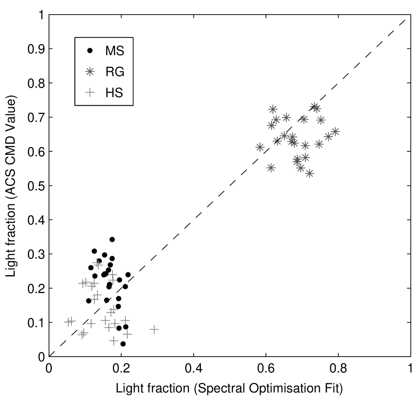
Figure 12: Light fractions of various evolutionary stages from the ACS CMDs as a function of those obtained by our population synthesis model. Fractions from main sequence (MS), red giant (RG), and “hot star” (HS) regions are shown as circles, stars, and crosses, respectively. The 1:1 relation is shown as a dashed line.

Regarding the fractions for individual clusters, we note that the HS fractions derived spectroscopically do not always agree with those from CMDs. This can be seen in Figure 12 where we show the light fractions of MS, RG, and HS from the ACS CMDs against our fitted results. While the agreement is generally very good, the scatter is large. The latter may result from the crudeness of our boundaries. For instance, our RG zone (see Figure 16) may contain some RHB stars that truly belong in the HS zone. This is especially true when the RHB is concentrated close to the RGB in the CMD (e.g. NGC 104, NGC 6441). Conversely, some MILES stars that fall in our HS zone but lie near the boundary may in fact belong to the RG zone (e.g. NGC 6752, NGC 7089). Thus in order to obtain accurate evolutionary phase fractions, the CMD zone boundaries must be carefully defined. See Appendix C for a visual representation on a per-cluster basis.

The test above is yet another important validation of our numerical optimisation spectral decomposition method.

4.3.2 Comparison of (V-I) Distributions

In order to compare the colour distributions based on our spectral decompositions and extracted from CMDs, we extract $V-I$ colours for MILES stars from the SIMBAD astronomical database. Because the latter lacks $I-$band magnitudes for many MILES stars, and short of any other catalogue with colour information, we use the colour interpolator of  Worthey & Lee (2011) to convert the atmospheric parameters $T_{\rm eff}$, $\log g$, and [Fe/H] for our final basis stars into $V-I$ colours.

A check on the reliability of the calculated values is performed by comparing the Worthey & Lee estimates with measured values from SIMBAD (if available). Modulo a small group of 5 discrepant stars (none of which are included in our final basis), the overall agreement is excellent. The mean difference in $V-I$ between the two datasets for stars in our basis is $-0.03$ with an rms dispersion of $0.11$. We thus verify the reliability of the Worthey $\&$ Lee calculator, as those authors also demonstrated in their paper.

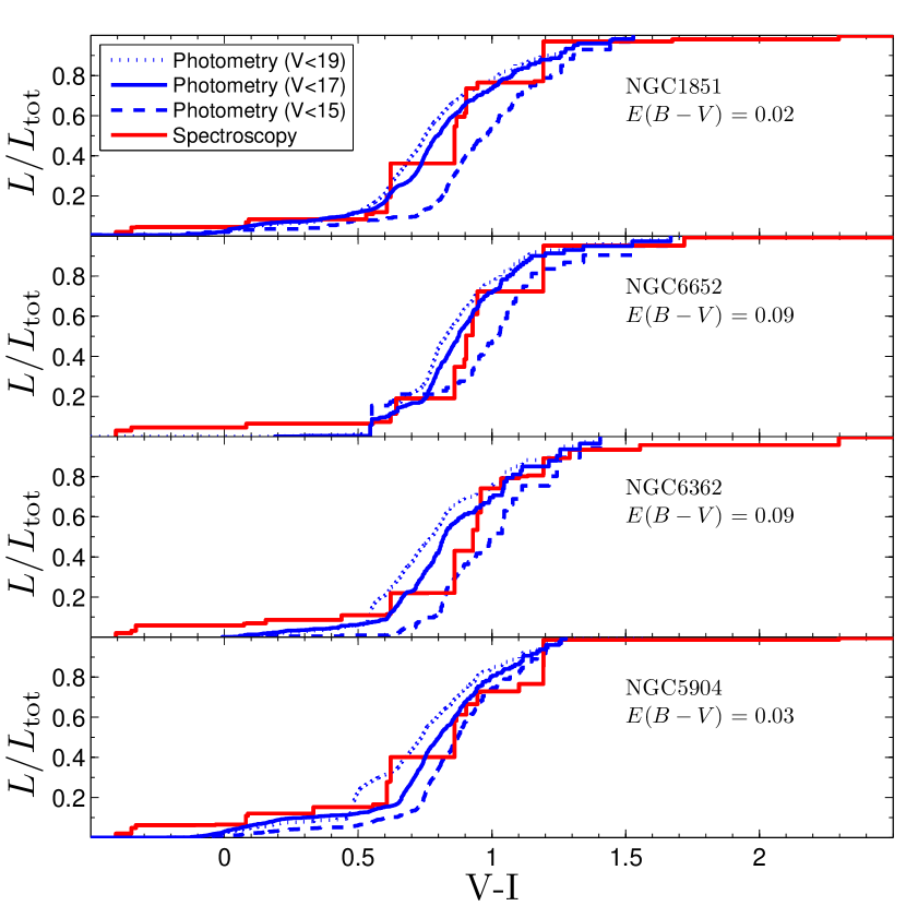
Figure 13: CDFs of the $V-I$ distributions obtained from our decompositions (red) compared to those from CMDs (blue) for a select sample of GGCs with low reddening. The CMD CDFs are shown for a range of the $V-$band magnitude cut-offs (see upper-left corner legend), as described in the text. The best match is obtained for a magnitude cut-off of $V<17$.

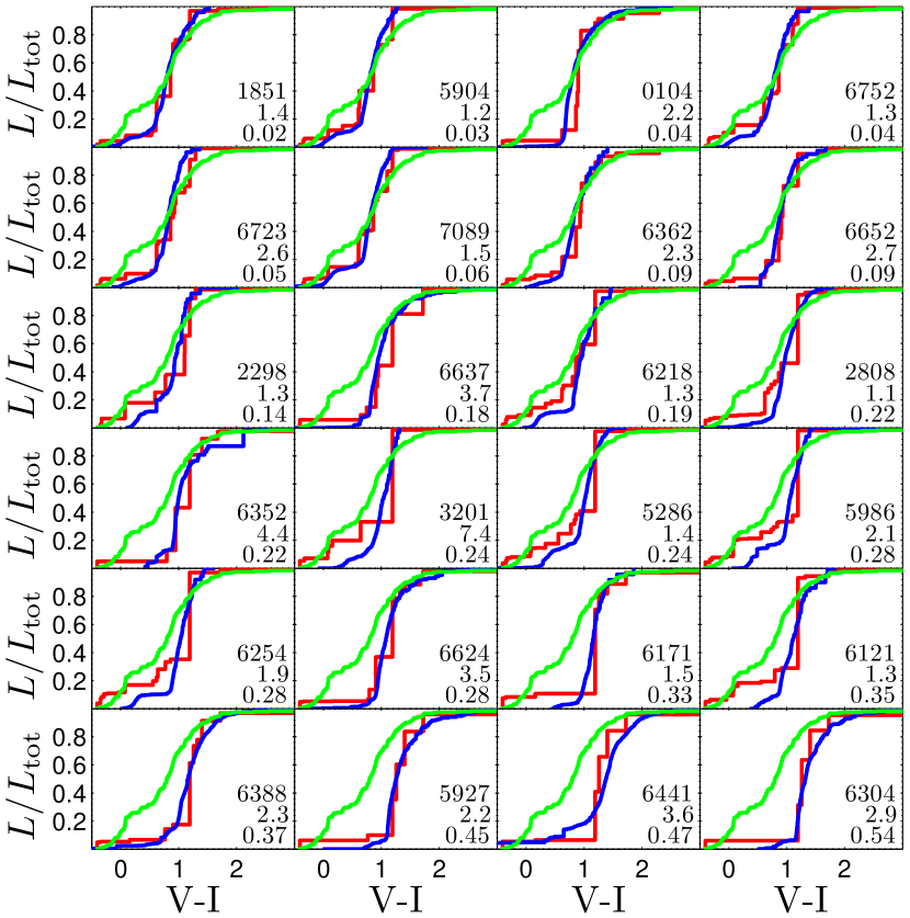
Figure 14: CDFs of the $V-I$ distributions obtained from our spectral optimisations (red), compared with those derived from CMDs (blue), for all the GGCs overlapping between the HST ACS (Sarajedini et al. 2007) and the S05 libraries. The colour distribution corresponding to equal weight for each star (i.e., initial conditions) is shown in green. NGC ID, $\chi^{2}$ value, and $E(B-V)$ from Harris (1996) are displayed at the bottom right of each panel (top to bottom, respectively).

The $V-I$ distributions from our spectral fits can now be compared with those extracted from the CMDs. This comparison uses the same method described in Section 3.2 for the mock spectra created from stars lying outside of our final basis.

A potential concern in this comparison is that our optimisation method may be insensitive to faint, cool stars that contribute little to the total integrated light in the GGC spectra. Such stars may strongly affect gravity-sensitive or molecular absorption features which only make up a few out of the thousands of pixels in the spectra, so fitting to the full spectrum may miss them. In an attempt to correct for this, we compute light fractions using only stars in the CMD brighter than some magnitude limit. We tested $V$-band magnitude cut-off values ranging from $V=$ 14 to 22 for each CMD-spectral optimisation comparison and found that the best match is found for an empirically-derived limit of $V<17$. Figure 13 shows this comparison for three values of $V-$band magnitude cutoff, where the CMD and optimisation CDFs are shown in blue and red, respectively. This threshold should not be adopted universally; it is merely representative of the sensitivity of our particular spectroscopic set-up.

The CDFs for the ACS clusters versus their $V-I$ distribution are shown in Figure 14, with the clusters arranged from the top-left to bottom-right corners in order of increasing $E(B-V)$. As gauged visually, the match between the CMD and optimisation CDFs is superb for most clusters.

This test further supports the applicability of our population synthesis method. However, some clusters, such as NGC 3201, 5986, and 6254, show large discrepancies in the bluer regions. Since these clusters have reasonably good fits (see Appendix A), this discrepancy may be the result of unknown method degeneracies.

5 Conclusions

We have tested the method of non-linear optimisation (population synthesis) to decompose the integrated spectra of stellar systems into distributions of fundamental stellar parameters. To this end, we have used the spectral MILES library (Sánchez-Blázquez et al. 2006) to construct a suitable basis for the optimisation. Our decomposition method was tested on mock spectra constructed from the spectral library basis, yielding relative uncertainties of 20 per cent in the light fractions and absolute total light noise levels of 5 per cent or less, for a given star.

The stellar atmospheric parameters $T_{\rm eff}$, $\log g$, and [Fe/H] of mock spectra constructed from stars outside our stellar basis were also extracted with great accuracy by our optimisation technique. The mean errors between mock and fitted atmospheric parameters are 240 K, 0.04 dex, and 0.03 dex for $T_{\rm eff}$, $\log g$, and [Fe/H], respectively.

Having established the reliability of our spectral decomposition method, we applied our code to the individual integrated spectra of 41 Galactic globular clusters from the collection of Schiavon et al. (2005). These spectra were decomposed into relative fractions (by light) of a suitably chosen basis of stellar spectra from the MILES library.

The light-weighted GGC metallicities obtained from population synthesis agree well with those of Harris (1996) and our own literature compilation (Schiavon et al. 2005) when an appropriate reddening model is included in the decomposition. In the absence of such a model, good agreement for highly reddened clusters is only found when the continuum is removed (i.e. only prominent absorption features enter the fit).

The decompositions based on our optimised population synthesis were compared with CMD data of the 24 S05 GGCs which overlap with those from Sarajedini et al. (2007). Our CMD analysis yielded light-weighted luminosity fractions for various stellar evolutionary stages as well as their $V-I$ colour distributions. We found superb agreement between these quantities and the luminosity fractions derived from our population synthesis optimisations. The extracted spectroscopic luminosity fractions are reported in the abstract and in Table 2 are compared against similar values from CMDs.

Overall, we find the technique of numerical optimisation to be a reliable tool for extracting the mean metallicity and light fractions of stellar populations in unresolved stellar systems. Some caveats pertaining to the depth of the spectroscopic data and the line of sight reddening must be taken into consideration.

Appendix A APPENDIX A

In this Appendix, we show the fits to our 41 GGC spectra from our population synthesis code. The S05 spectra and their optimisation fits are shown in blue and red, respectively. Goodness of fit is indicated by $\chi^{2}$/dof values and data-model residuals are shown in the inset below each spectrum. To estimate $\chi^{2}$/dof, the errors in each GGC spectrum were computed pixel-to-pixel by dividing the spectrum by the S/N ratio spectra provided by S05. Metallicity and reddening values from the 2010 version of Harris (1996) and from our fits are also indicated on each panel.

Spectral optimisation fits to GGC spectra.

…/continued

…/continued

…/continued

…/continued

…/continued

…/continued

…/continued

…/continued

…/continued

…/continued

…/continued

…/continued

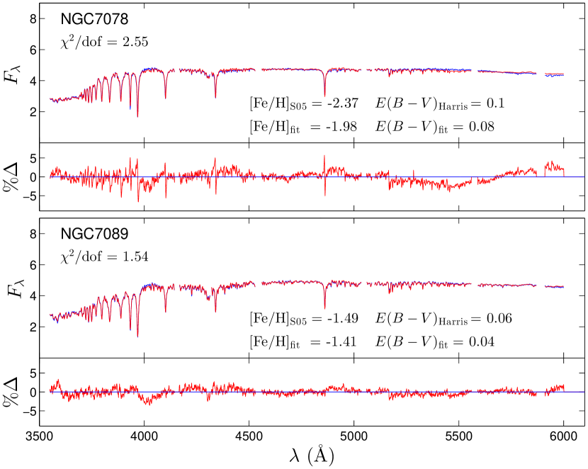
Figure 15: …/continued

Appendix B APPENDIX B

The $V$-band luminosity fractions of the many stellar evolutionary phases for the 24 ACS GGC clusters are displayed graphically in Figure 16. The light fractions of main sequence (MS), turn-off (TO), subgiant branch (SGB), and blue straggler (BS) stars remain fairly constant with [Fe/H]. Conversely, the red and asymptotic giant branch (RGB and AGB respectively) light fractions seem to decrease with increasing GGC metallicity. The fairly smooth and real increase and decrease of the red and blue horizontal branch (RHB and BHB, respectively) light fractions with metallicity, especially from [Fe/H] = -1.4 to -1, is a well-known dependence of the horizontal branch morphology. Note that our data would only be weakly sensitive to any second-order dependence of HB morphology (Sarajedini 1992).

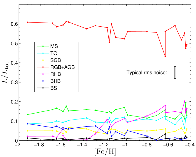
Figure 16: Fractional contributions of different stellar evolutionary phases to the total light of the 24 GGCs from Sarajedini et al. (2007) overlapping with S05, as a function of cluster metallicity. Evolutionary phases include turn-off (TO), subgiant branch (SGB), red giant and asymptotic giant branch (RGB+AGB), red horizontal branch (RHB), blue horizontal branch (BHB), and blue stragglers (BS). The rms noise in the luminosity fractions of turn-off stars is shown on the figure as a representative uncertainty.

Appendix C APPENDIX C

In this Appendix, we present colour-magnitude diagrams for the 24 GGCs of Sarajedini et al. (2007) which coincide with those studied by S05. Stages of stellar evolution are indicated by distinct boxes while the per cent contribution of each stage to the total luminosity of the cluster is provided in the legend. The uncertainty in the displayed luminosity fractions is estimated at 6 per cent, based on the rms noise in the luminosity fractions of the red giant stars.

Also included are CMDs of the same clusters, constructed through our optimised decompositions of their integrated spectra. Point sizes indicate the relative light-weighted contribution to the integrated spectra.

Colour-magnitude diagrams of GGCs; results are displayed as in Figure 9. The top and bottom panels correspond to CMDs from Sarajedini et al. (2007) and MILES, respectively.

…/continued

…/continued

…/continued

…/continued

…/continued

…/continued

…/continued

…/continued

…/continued

…/continued

…/continued

…/continued

…/continued

…/continued

…/continued

…/continued

…/continued

…/continued

…/continued

…/continued

…/continued

…/continued

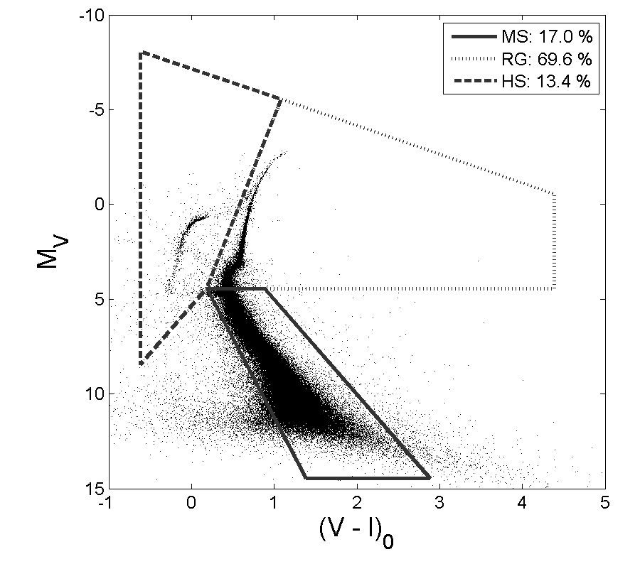
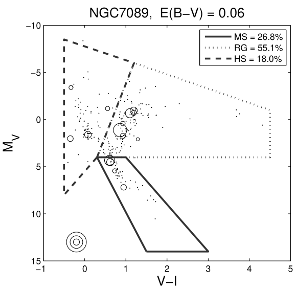
Figure 17: …/continued

Appendix D APPENDIX D

Here we present the ACS colour-magnitude diagrams for GGCs as in Appendix C, except that our evolutionary zones are now more precisely defined.

Galactic globular cluster colour-magnitude diagrams.

…/continued

…/continued

…/continued

…/continued

…/continued

…/continued

…/continued

…/continued

…/continued

…/continued

…/continued

…/continued

…/continued

…/continued

…/continued

…/continued

…/continued

…/continued

…/continued

…/continued

…/continued

…/continued

…/continued

References

- Bruzual & Charlot (1993) Bruzual G., Charlot S., 1993, ApJ, 405, 538
- Buzzoni (1989) Buzzoni A., 1989, ApJS, 71, 817
- Cardelli et al. (1989) Cardelli J. A., Clayton G. C., Mathis J. S., 1989, ApJ, 345, 245
- Carretta et al. (2009) Carretta E., Bragaglia A., Gratton R., D’Orazi V., Lucatello S., 2009, A&A, 508, 695
- Carretta & Gratton (1997) Carretta E., Gratton R. G., 1997, A&AS, 121, 95
- Cenarro et al. (2007) Cenarro A. J., Peletier R. F., Sánchez-Blázquez P., Selam S. O., Toloba E., Cardiel N., Falcón-Barroso J., Gorgas J., Jiménez-Vicente J., Vazdekis A., 2007, MNRAS, 374, 664
- Cezario et al. (2013) Cezario E., Coelho P. R. T., Alves-Brito A., Forbes D. A., Brodie J. P., 2013, A&A, 549, A60
- Cid Fernandes et al. (2005) Cid Fernandes R., Mateus A., Sodré L., Stasińska G., Gomes J. M., 2005, MNRAS, 358, 363
- Conroy et al. (2009) Conroy C., Gunn J. E., White M., 2009, ApJ, 699, 486
- Faber (1972) Faber S. M., 1972, A&A, 20, 361
- Falcón-Barroso et al. (2011) Falcón-Barroso J., Sánchez-Blázquez P., Vazdekis A., Ricciardelli E., Cardiel N., Cenarro A. J., Gorgas J., Peletier R. F., 2011, A&A, 532, A95+
- Harris (1996) Harris W. E., 1996, AJ, 112, 1487
- Koleva et al. (2009) Koleva M., Prugniel P., Bouchard A., Wu Y., 2009, A&A, 501, 1269
- Koleva et al. (2008) Koleva M., Prugniel P., Ocvirk P., Le Borgne D., Soubiran C., 2008, MNRAS, 385, 1998
- Kraft & Ivans (2003) Kraft R. P., Ivans I. I., 2003, PASP, 115, 143
- MacArthur (2005) MacArthur L. A., 2005, ApJ, 623, 795
- MacArthur et al. (2009) MacArthur L. A., González J. J., Courteau S., 2009, MNRAS, 395, 28
- Maraston (1998) Maraston C., 1998, MNRAS, 300, 872
- Maraston (2007) Maraston C., 2007, in Combes F., Palouš J., eds, IAU Symposium Vol. 235 of IAU Symposium, Stellar Population Models. pp 52–56
- Maraston & Thomas (2000) Maraston C., Thomas D., 2000, ApJ, 541, 126
- Moultaka (2005) Moultaka J., 2005, A&A, 430, 95
- O’Connell (1976) O’Connell R. W., 1976, ApJ, 206, 370
- Ocvirk et al. (2006) Ocvirk P., Pichon C., Lançon A., Thiébaut E., 2006, MNRAS, 365, 46
- Pickles (1985) Pickles A. J., 1985, ApJ, 296, 340
- Prugniel et al. (2011) Prugniel P., Vauglin I. Koleva M., 2011, VizieR Online Data Catalog, 353, 19165
- Renzini (1981) Renzini A., 1981, Annales de Physique, 6, 87
- Roediger et al. (2014) Roediger J. C., Courteau S., Graves G., Schiavon R. P., 2014, ApJS, 210, 10
- Sánchez-Blázquez et al. (2006) Sánchez-Blázquez P., Peletier R. F., Jiménez-Vicente J., Cardiel N., Cenarro A. J., Falcón-Barroso J., Gorgas J., Selam S., Vazdekis A., 2006, MNRAS, 371, 703
- Sarajedini (1992) Sarajedini A., 1992, PhD thesis, Yale University., New Haven, CT.
- Sarajedini et al. (2007) Sarajedini A., Bedin L. R., Chaboyer B., Dotter A., Siegel M., Anderson J., Aparicio A., King I., Majewski S., Marín-Franch A., Piotto G., Reid I. N., Rosenberg A., 2007, AJ, 133, 1658
- Schiavon (2007) Schiavon R. P., 2007, ApJS, 171, 146
- Schiavon et al. (2005) Schiavon R. P., Rose J. A., Courteau S., MacArthur L. A., 2005, ApJS, 160, 163
- Soubiran et al. (1998) Soubiran C., Katz D., Cayrel R., 1998, A&AS, 133, 221
- Spinrad & Taylor (1971) Spinrad H., Taylor B. J., 1971, ApJS, 22, 445
- Tojeiro et al. (2007) Tojeiro R., Heavens A. F., Jimenez R., Panter B., 2007, MNRAS, 381, 1252
- Vergely et al. (2002) Vergely J.-L., Lançon A., Mouhcine 2002, A&A, 394, 807
- Walcher et al. (2006) Walcher C. J., Böker T., Charlot S., Ho L. C., Rix H.-W., Rossa J., Shields J. C., van der Marel R. P., 2006, ApJ, 649, 692
- Worthey et al. (1994) Worthey G., Faber S. M., Gonzalez J. J., Burstein D., 1994, ApJS, 94, 687
- Worthey & Lee (2011) Worthey G., Lee H.-c., 2011, ApJS, 193, 1