Seed Photon Fields of Blazars in the Internal Shock Scenario

Abstract

We extend our approach of modeling spectral energy distribution (SED) and lightcurves of blazars to include external Compton (EC) emission due to inverse Compton scattering of an external anisotropic target radiation field. We describe the time-dependent impact of such seed photon fields on the evolution of multifrequency emission and spectral variability of blazars using a multi-zone time-dependent leptonic jet model, with radiation feedback, in the internal shock model scenario.

We calculate accurate EC-scattered high-energy spectra produced by relativistic electrons throughout the Thomson and Klein-Nishina regimes. We explore the effects of varying the contribution of (1) a thermal Shakura-Sunyaev accretion disk, (2) a spherically symmetric shell of broad-line clouds, the broad line region (BLR), and (3) a hot infrared emitting dusty torus (DT), on the resultant seed photon fields. We let the system evolve to beyond the BLR and within the DT and study the manifestation of the varying target photon fields on the simulated SED and lightcurves of a typical blazar. The calculations of broadband spectra include effects of $\gamma-\gamma$ absorption as $\gamma$-rays propagate through the photon pool present inside the jet due to synchrotron and inverse Compton processes, but neglect $\gamma-\gamma$ absorption by the BLR and DT photon fields outside the jet. Thus, our account of $\gamma-\gamma$ absorption is a lower limit to this effect. Here, we focus on studying the impact of parameters relevant for EC processes on high-energy (HE) emission of blazars.

1 Introduction

Blazars are known for their highly variable broadband emission. They are characterized by a doubly humped spectral energy distribution (SED), attributed to non-thermal emission, and spectral variability. The SED and variability patterns can be used as key observational features to place constraints on the nature of the particle population, acceleration of particles, and the environment around the jet that is responsible for the observed emission. Conversely, incorporating the nature of the particle population and the jet environment, as accurately as possible, in modeling such observational features can enable us to reach a better agreement between theoretical and observational results. Thus, exploring the environment of a blazar jet in an anisotropic and time-dependent manner is important for connecting the pieces together and putting tighter constraints on the origin of $\gamma$-ray emission.

Blazars, a combination of BL Lacertae (BL Lac) objects and flat spectrum radio-loud quasars (FSRQs), are divided into various subclasses depending on the location of the peak of the low-energy (synchrotron) SED component. The synchrotron peak lies in the infrared regime, with $\nu_{\rm s}\leq 10^{14}$ Hz, in low-synchrotron-peaked (LSP) blazars comprising FSRQs and low-frequency peaked BL Lac objects (LBLs). In the case of intermediate-synchrotron-peaked (ISP) blazars, consisting of LBLs and intermediate-frequency peaked BL Lacs (IBLs), the synchrotron peak lies in the optical - near-UV region with $10^{14}<\nu_{\rm s}\leq 10^{15}$ Hz. The synchrotron component of high-synchrotron-peaked (HSP) blazars, which include essentially all high-frequency-peaked BL Lac objects (HBLs), peaks in the X-rays at $\nu_{\rm s}>10^{15}$ Hz (Abdo et al., 2010; Böttcher, 2012). The high-energy (HE) component of blazars can be a result of inverse Compton (IC) scattering of synchrotron photons internal to the jet resulting in synchrotron self-Compton (SSC) emission (Bloom & Marscher, 1996). It could also be due to upscattering of accretion-disk photons (Dermer & Schlickeiser, 1993), and/or photons initially from the accretion disk being scattered by the broad-line region (BLR) (Sikora et al., 1994; Dermer, Sturner, & Schlickeiser, 1997), and/or seed photons from a surrounding dusty torus (DT) (Kataoka et al., 1999; Błażejowski et al., 2000). In the case of HBLs, the HE component is usually well reproduced with a synchrotron/SSC leptonic jet model (e.g., Finke, Dermer, & Böttcher, 2008; Aleksić et al., 2012), whereas an additional external Compton (EC) component is almost always required to fit the high-energy spectra of FSRQs, LBLs, and IBLs (e.g., Chiaberge & Ghisellini, 1999; Collmar et al., 2010).

Detailed numerical calculations for Compton scattering processes have been carried out for many specific models of blazar jet emission that involve their environment. Dermer & Schlickeiser (1993, 2002) have calculated Compton scattering of target photons in the Thomson regime from an optically thick and geometrically thin, thermal accretion disk based on the model of Shakura & Sunyaev (1973). Quasi-isotropic seed photon fields due to BLR or DT have also been considered to obtain Compton-scattered high-energy spectra in the Thomson limit by several authors (Sikora et al., 1994; Dermer, Sturner, & Schlickeiser, 1997; Błażejowski et al., 2000). On the other hand, extensive calculations involving anisotropic accretion-disk and BLR seed photon fields have been considered as well (Böttcher, Mause, & Schlickeiser, 1997; Böttcher & Bloom, 2000; Böttcher & Reimer, 2004; Kusunose & Takahara, 2005). Anisotropic radiation fields of the disk, the BLR, and the DT have been studied previously by Donea & Protheroe (2003), but primarily in the context of $\gamma-\gamma$ interaction of these photons with the GeV and TeV photons produced in the jet. Anisotropic treatment of BLR and DT photons, focussing on jet emission and rapid non-thermal flares, was carried out by Sokolov & Marscher (2005). These authors studied parameters describing the properties of BLR and DT that govern the interplay between the dominance of SSC and EC emission and their subsequent impact on SEDs, as well as relative time delays between light curves at different frequencies. For the purposes of their study, they used an integrated intensity - instead of considering line and continuum intensities separately - of the incident emission from the BLR. The emitting plasma was assumed to be located at parsec scales and the evolution of HE emission at sub-pc distances was ignored.

Recently, anisotropic treatment of disk and BLR target radiation fields has been considered by Dermer et al. (2009). The authors have calculated accurate $\gamma$-ray spectra due to inverse Comptonization of such seed photon fields throughout the Thomson and Klein-Nishina (KN) regimes to model FSRQ blazars, although in a one-zone scenario. Also, these authors evolve the system to only sub-pc distances along the jet axis, limiting themselves to locations within the BLR. In addition to this, one-zone leptonic jet models were recently shown (Böttcher, Reimer, & Marscher, 2009) to have severe limitations in attempts to reproduce very high energy (VHE) flares, such as that of 3C 279 detected in 2006 (Albert et al., 2008).

In a more recent approach, Marscher (2013) has considered an anisotropic seed photon field of the DT to calculate the resultant EC component of HE emission from blazar jets, in a turbulent extreme multi-zone scenario. While the $\gamma$-ray spectra are calculated throughout the Thomson and KN regimes, the energy loss rates are limited to only the Thomson regime. For the problem that work addresses, the system is located beyond the BLR, at parsec-scale distances from the central engine.

Here, we extend the previous approach of Joshi & Böttcher (2011, hereafter Paper 1), which calculated the synchrotron and SSC emission from blazar jets, to address some of the limitations of the models mentioned above. We use a fully time-dependent, 1-D multi-zone with radiation feedback, leptonic jet model in the internal shock scenario, shortened to the MUlti ZOne Radiation Feedback, MUZORF, model. We evolve the system from sub-pc to pc scale distances along the jet axis. We consider anisotropic target radiation fields to calculate the HE spectra resulting from EC scattering processes. The entire spectrum is calculated throughout the Thomson and KN regimes, thereby making it applicable to all classes of blazars. We include the attenuation of jet $\gamma$-rays through $\gamma-\gamma$ absorption (described in Paper 1) due to the presence of target radiation fields inside the jet, in a self-consistent manner. The generalized approach of our model lets us account for the constantly changing contribution of each of the seed photon field sources in producing HE emission in a self-consistent and time-dependent manner. This is especially relevant for understanding the origin of $\gamma$-ray emission from blazar jets.

In a number of previous analyses, the region within the BLR has been considered the most favorable location for $\gamma$-ray emission, with a range limited to between 0.01 and 0.3 pc Dermer & Schlickeiser (1994); Blandford & Levinson (1995); Ghisellini & Madau (1996). The reason behind this is the short intra-day variability timescales observed in some $\gamma$-ray flares, which indicated on the basis of light crossing timescales that the emission region is small and hence not be too far away from the central engine Ghisellini & Madau (1996); Ghisellini & Tavecchio (2009). At the same time, the emission region cannot be too close to the central engine without violating constraints placed by the $\gamma-\gamma$ absorption process Ghisellini & Madau (1996); Liu & Bai (2006). As a result, an emission region location closer to the BLR was considered the most favorable position due to the strong dependence of the scattered flux on the level of boosting and the energy of incoming photons (Sikora et al., 1994). Contrary to the above scenario, recent observations have shown coincidences of $\gamma$-ray outbursts with radio events on pc scales (e.g., León-Tavares et al., 2012; Jorstad et al., 2013). This seems to suggest a cospatial origin of radio and $\gamma$-ray events located at such distances. As a result, some authors conclude that the $\gamma$-ray emitting region could also lie outside of the BLR Sokolov & Marscher (2005); Lindfors, Valtaoja, & Türler (2005).

Thus, in order to understand the origin of $\gamma$-ray emission, it is important to let the system being modeled evolve to beyond the BLR and into the DT, and to include its contribution to the production of $\gamma$-ray emission. Here, we focus our attention toward understanding the dependence of $\gamma$-ray emission on the combination of various intrinsic physical parameters. We explore this aspect by including various components of seed photon fields in order to obtain a complete picture of their contribution in producing $\gamma$-ray emission and understand their effects on the dynamic evolution of SEDs and spectral variability patterns.

In §2, we describe our EC framework of including anisotropic seed photon fields from the accretion-disk, the BLR, and the DT. We lay out the expressions used to calculate accurate Compton-scattered $\gamma$-ray spectra resulting from the seed photon fields and the corresponding electron energy loss rates throughout the Thomson and KN regimes. In §3, we describe our baseline model, its simulated results, and the relevant physical input parameters that we use in the study. In §3.2, we present our results of the parameter study and discuss the effects of varying the input parameters on the simulated SED and lightcurves. We discuss and summarize our findings in §4. Throughout this paper, we refer to $\alpha$ as the energy spectral index such that flux density, $F_{\nu},\propto\nu^{-\alpha}$; the unprimed quantities refer to the rest frame of the AGN (lab frame), primed quantities to the comoving frame of the emitting plasma, and starred quantities to the observer’s frame; the dimensionless photon energy is denoted by $\epsilon=\frac{h\nu}{m_{\rm e}c^{2}}$.

Appendix A delineates the details of line-of-sight calculations for the BLR line and diffuse continuum emission used in obtaining the intensity of incoming BLR photons.

2 Methodology

We consider a multi-zone time-dependent leptonic jet model with radiation-feedback scheme as described in Paper 1. We extend our previous model of synchrotron/SSC emission to include the EC component in order to simulate the SED and spectral variability patterns of blazars. We consider three sources of external seed photon fields, namely the accretion disk, the BLR, and the DT. We evolve the emission region in the jet from sub-pc to pc scales (within the DT) and follow the evolution of the SED and spectral variability patterns over a period of $\sim$ 1 day, corresponding to the timescale of a rapid nonthermal flare. Such a comprehensive approach can be used as an important tool for connecting the origin of $\gamma$-ray emission of a flare to its multiwavelength properties.

As in paper 1, we consider a cylindrical emission region for our current study. We assume the emitting volume to be well collimated out to pc distances, which is a safe assumption to make based on the work of Jorstad et al. (2005), and hence do not consider the effects of adiabatic expansion on the evolution of the strength of the magnetic field or the electron population in the emission region. The size of the emission region is assumed to be small in comparison to the sizes of and distances to the external seed photon field sources. This way, the external radiation can be safely assumed to be homogeneous throughout the emitting plasma, although it is still highly anisotropic in the comoving frame of the plasma. In our current framework, we do not simulate radio emission as the calculated flux is well below the actual radio value. This is because we follow the early phase of $\gamma$-ray production corresponding to a shock position upto $\sim$ 1 pc in the lab frame. During this phase, the emission region is highly optically thick to GHz radio frequencies.

The angular dependence of the incoming radiation and the amount to which it contributes toward EC emission is determined by the geometry of all three seed photon field sources and the location of the emission region along the jet axis. In addition, the anisotropy is further enhanced due to relativistic aberration and Doppler boosting or deboosting in the plasma frame. We assume the external radiation to be constant in time over the period of our simulation. Figure 1 depicts the geometry of all three external sources under consideration. The jet is oriented along the z-axis in a plane perpendicular to the plane of the central engine, which is composed of the black hole and the accretion disk surronding it. The central engine is enveloped by a BLR, considered to be a geometrically thick spherical shell, and is situated inside the cavity of the BLR. These sources are, in turn, encased by a puffed up torus containing hot dust.

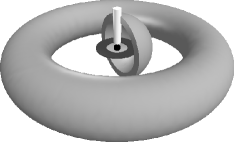
Figure 1: Illustration of the three sources of external radiation influencing the high-energy emission from the jet of a blazar. The central engine and the DT are situated in the same plane while the jet and the polar axis of the BLR lie in a plane perpendicular to it. Only half of the BLR is shown to illustrate the location of the central engine in the spherical shell’s cavity.

In the following subsections, we discuss the sources of seed photons for EC scattering and delineate the expressions that we use to calculate the corresponding emissivities and energy loss rates throughout the Thomson and KN regimes.

2.1 The Accretion Disk

In order to calculate the EC scattering of photons coming directly from a central source, we consider an optically thick accretion disk that radiates with a blackbody spectrum, based on the model of Shakura & Sunyaev (1973). The blackbody spectrum is calculated according to a temperature distribution T(R) given by Eq. (4) of Böttcher, Mause, & Schlickeiser (1997). where R is the radius of the disk.

Figure 2 shows a schematic of the disk geometry and the angular dependence of the disk spectral intensity on the position of the emission region in the jet. We assume a multi-color disk and calculate the radius dependent quantity, $\Theta(\rm R)\equiv k_{B}T(R)/m_{e}c^{2}$ (where $k_{B}=1.38\times 10^{-16}$ erg/K is the Boltzmann constant), in order to obtain the EC emissivity and the corresponding electron energy loss rate. The disk is assumed to emit in the energy range from optical to hard X-rays (10 keV), with a characteristic peak frequency of $\nu^{\rm peak}_{\rm disk}\sim 2\times 10^{15}$ Hz.

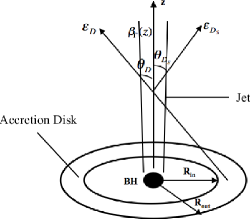
Figure 2: Model for the disk-jet geometry used in our EC formulation. The accretion disk extends from inner, $R_{\rm in}$, to outer, $R_{\rm out}$ radius. Temperature of the disk is calculated for all radii between $R_{\rm in}$ and $R_{\rm out}$. The emission region is located inside the jet, moving along the z-axis with a velocity $\beta_{\Gamma_{\rm sh}}c$ (as described in Paper 1). The incoming photon of dimensionless energy $\epsilon_{\rm D}$ from the disk intercepts the emitting volume at an angle $\theta_{\rm D}$ and the resulting outgoing photon with energy $\epsilon_{\rm D_{\rm S}}$ is scattered at an angle $\theta_{\rm D_{\rm S}}$.

For sake of brevity, the subscript $D$ has been dropped from $\epsilon$ for the rest of this section. Now, the spectral surface energy flux at radius R is given by $F(\nu,R)(erg~{}cm^{-2}s^{-1}Hz^{-1})=\pi B_{\nu}[T(R)]$, where $B_{\nu}[T(R)]$ describes the spectrum of a blackbody radiation at radius R with temperature T(R) (Dermer & Schlickeiser, 1993). The differential number of photons produced per second between $\epsilon$ and $\epsilon+d\epsilon$ and emitted from disk radius R and R + dR, $\dot{N}(\epsilon,R)$, is given by

$$\frac{dN}{dRdtd\epsilon}=\frac{2\pi^{2}RB_{\nu}[T(R)]}{h\epsilon}~{},$$ (1)

where $B_{\nu}[T(R)]=\frac{2h}{c^{2}}\frac{\nu^{3}}{\exp{[h\nu/k_{B}T(R)]}-1}$.

The differential spectral photon number density, $n_{\rm ph}(\epsilon,R)~{}(cm^{-3}\epsilon^{-1}R^{-1})$, is then given by

$$\frac{dn_{\rm ph}}{d\epsilon dR}=\frac{\dot{N}(\epsilon,R)}{4\pi x^{2}c}=\frac{\pi}{2}R\frac{B_{\nu}[T(R)]}{x^{2}ch\epsilon}~{},$$ (2)

where $x=\sqrt{R^{2}+z^{2}}$ and $\cos\theta_{D}=\eta_{\rm ph}=z/x$. Here and in the rest of the paper, a quantity is differential in the variables that are listed in parentheses. If the variables are preceded by a semicolon or only one variable is listed in the parentheses, then the quantity is parametrically dependent on such variable(s).

Converting $n_{\rm ph}(\epsilon,R)$ into $n_{\rm ph}(\epsilon,\Omega)$ by realizing that $\eta_{\rm ph}=\frac{z}{\sqrt{R^{2}+z^{2}}}$ and assuming azimuthal symmetry of the photon source, $n_{\rm ph}(\epsilon,\Omega_{\rm ph})$ is given by

$$\frac{dn_{\rm ph}}{d\epsilon d\Omega_{\rm ph}}=\frac{1}{2\pi}\frac{\pi B_{\nu}[T(R)]}{2ch\epsilon\eta_{\rm ph}}~{}.$$ (3)

Using Eq. (3) and the invariance of $\frac{n_{\rm ph}(\epsilon,\Omega)}{\epsilon^{2}}$ (Rybicki & Lightman, 1979; Dermer & Schlickeiser, 1993; Böttcher, Mause, & Schlickeiser, 1997),

$$n_{\rm ph}^{\prime}(\epsilon^{\prime},\Omega_{\rm ph}^{\prime})=\frac{\epsilon^{\prime 2}}{\epsilon^{2}}n_{\rm ph}(\epsilon,\Omega_{\rm ph})~{},$$ (4)

we can obtain the anisotropic differential spectral photon number density, $n_{\rm ph}^{\prime}(\epsilon^{\prime},\Omega_{\rm ph}^{\prime})$, in the plasma frame (Böttcher, Mause, & Schlickeiser, 1997)

$$n_{\rm ph}^{\prime}(\epsilon^{\prime},\Omega_{\rm ph}^{\prime})=\frac{1}{2c^{3}}(\frac{m_{e}c^{2}}{h})^{3}\epsilon^{\prime 2}\left(e^{\frac{\epsilon^{\prime}\Gamma_{\rm sh}(1+\beta_{\Gamma_{\rm sh}}\eta^{\prime}_{\rm ph})}{\Theta(R)}}-1\right)^{-1}\frac{1+\beta_{\Gamma_{\rm sh}}\eta^{\prime}_{\rm ph}}{\eta^{\prime}_{\rm ph}+\beta_{\Gamma_{\rm sh}}}~{},$$ (5)

Here, $\eta^{\prime}_{\rm ph}=\frac{z-\beta_{\Gamma_{\rm sh}}x}{x-\beta_{\Gamma_{\rm sh}}z}$ is the cosine of the angle that the incoming photon, emitted at radius $R$, makes with respect to the jet axis at height z. The relevant Lorentz transformations are given by (Dermer & Schlickeiser, 1993)

$$\epsilon=\epsilon^{\prime}\Gamma_{\rm sh}(1+\beta_{\Gamma_{\rm sh}}\eta^{\prime}_{\rm ph})$$

$$\eta_{\rm ph}=\frac{\eta^{\prime}_{\rm ph}+\beta_{\Gamma_{\rm sh}}}{1+\beta_{\Gamma_{\rm sh}}\eta^{\prime}_{\rm ph}}~{}.$$ (6)

The electron energy loss rate and photon production rate per unit volume due to inverse-Compton scattering of disk photons (ECD) can be calculated using Eq. (5). We use the approximation given in Böttcher, Mause, & Schlickeiser (1997) to calculate the energy loss rate of an electron with energy $\gamma^{\prime}$ throughout the Thomson and KN regimes:

$$-\dot{\gamma^{\prime}}_{\rm ECD}=\frac{\pi^{5}r_{e}^{2}}{30c^{2}}\left(\frac{m_{e}c^{2}}{h}\right)^{3}\gamma^{\prime 2}\Gamma_{\rm sh}^{2}\int\limits_{R_{\rm min}}^{R_{\rm max}}dR~{}\Theta^{4}(R)~{}R\frac{(x-\beta_{\Gamma_{\rm sh}}z)^{2}}{x^{4}}I(\langle\epsilon^{\prime}\rangle,\gamma^{\prime},\eta_{\rm ph}^{\prime})~{},$$ (7)

where, $I(\epsilon^{\prime},\gamma^{\prime},\eta_{\rm ph}^{\prime})$ is given by either equation (15) or (16) of Böttcher, Mause, & Schlickeiser (1997) according to the regime it is being calculated in.

On the other hand, if all scattering occurs in the Thomson regime, $\gamma^{\prime}\epsilon^{\prime}\ll 1$, then the electron energy loss rate can be directly calculated using Eq. (12) of Böttcher, Mause, & Schlickeiser (1997). Figure 3 shows a comparison between the electron energy loss rate obtained using the full expression given in Eq. (7) and the Thomson expression using Eq. (12) of Böttcher, Mause, & Schlickeiser (1997) for ECD. The transition from the KN to Thomson regime is governed by the temperature of the accretion disk such that the transition electron Lorentz factor is given by $\gamma_{\rm KN}\sim 1/(5\times 10^{-10}[T_{\rm max}/K])$, where $T_{\rm max}(K)=0.127\left[3GM\dot{M}/(8\pi\sigma_{\rm SB}R_{g}^{3})\right]^{1/4}$ is the maximum temperature of the disk for a non-rotating black hole (BH). The quantity $R_{\rm g}=\frac{GM}{c^{2}}$ is the gravitational radius corresponding to a BH of mass M (in units of $M_{\odot}$). The accretion rate of the BH is given by $\dot{M}$ such that the total disk luminosity, $L_{\rm disk}$, and the accretion efficiency, $\eta$, are related to $\dot{M}$ as $L_{\rm disk}=\eta\dot{M}c^{2}$. The Stefan-Boltzmann constant, $\sigma_{\rm SB}=5.6704\times 10^{-5}~{}erg~{}cm^{-2}K^{-4}s^{-1}$. In the case of our baseline model, $T_{\rm max}=9.6\times 10^{4}K$, implying $\gamma_{\rm KN}\sim 2\times 10^{4}$.

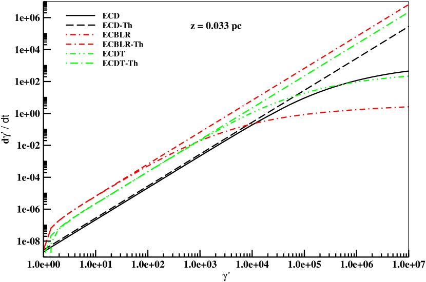
Figure 3: Energy loss rates of electrons/positrons showing a comparison of Thomson and full expressions due to inverse Comptonization of disk photons (ECD), BLR photons (ECBLR), and dusty torus photons (ECDT) in the forward shock (FS) region of the emitting volume at a distance of 0.033 pc from the BH. Input parameters of the base set (see §3) have been used to obtain the respective -$\dot{\gamma}^{\prime}$. The ECD process is denoted by solid line while its Thomson regime counterpart (ECD-Th) is depicted by long-dashed line. The ECBLR process is denoted by dot-dashed line and the ECBLR-Th process is represented by dot- double-short-dashed line. The ECDT process is represented by double-dot -dashed line and the ECDT-Th process is denoted by dot- double-long-dash line.

As can be seen from the figure, the lines for ECD and ECD-Th do not overlap each other in the Thomson regime. This is due to the fact that Eq. (13) of Böttcher, Mause, & Schlickeiser (1997) was used to calculate the electron energy loss rate due to external Comptonization of disk photons. The expression employs an approximation for all electron energies in calculating the electron energy loss rate. According to the approximation, the exact value of the angle between the electron and the jet axis does not play an important role and could be taken to be perpendicular to the jet axis for all electron energies. Furthermore, the thermal spectrum emitted by each radius of the disk could be approximated by a delta function in energy. Hence, the resulting electron energy loss rate is slightly different from that obtained using the full KN cross-section for an extended source.

The Compton photon production rate per unit volume, in the head-on approximation with $\beta_{\gamma^{\prime}}\rightarrow 1$, can be calculated from Eqs. (23) and (25) of Dermer et al. (2009). Using the following relationship between spectral luminosity, emissivity, and photon production rate per unit volume (Dermer & Menon, 2009), we obtain

$$\epsilon L(\epsilon,\Omega)=V_{b}\epsilon j(\epsilon,\Omega)$$

$$\epsilon j(\epsilon,\Omega)=m_{e}c^{2}\epsilon^{2}\dot{n}(\epsilon,\Omega)~{}.$$ (8)

After substituting the expression from Eq. (5), and converting $\eta_{\rm ph}^{\prime}$ in terms of R as mentioned above, we can obtain the ECD photon production rate per unit volume, in the plasma frame, under the head-on approximation as

$$\dot{n}_{\rm ECD}^{\prime}(\epsilon_{s}^{\prime},\Omega_{s}^{\prime})=\frac{3\sigma_{T}}{64\pi c^{2}}\frac{1}{\Gamma_{\rm sh}^{2}}\int\limits_{0}^{2\pi}d\phi^{\prime}_{\rm ph}\int\limits_{R_{\rm in}}^{R_{\rm out}}dR\frac{R}{(x-\beta_{\Gamma_{\rm sh}}z)^{2}}$$

$$\int\limits_{0}^{\epsilon^{\prime}_{\rm max}}d\epsilon^{\prime}\frac{\epsilon^{\prime}}{e^{\frac{\epsilon^{\prime}x}{\Theta(R)\Gamma_{\rm sh}(x-\beta_{\Gamma_{\rm sh}}z)}}-1}\int\limits_{\gamma^{\prime}_{\rm low}}^{\infty}d\gamma^{\prime}\frac{n^{\prime}_{e}(\gamma^{\prime})}{\gamma^{{}^{\prime}2}}\Xi_{\rm C}~{},$$ (9)

where the subscript $S$ stands for Compton scattered quantities, $\sigma_{T}=6.65\times 10^{-25}cm^{2}$ is the Thomson cross-section for an electron, and $n^{\prime}_{e}(\gamma^{\prime})$ is the electron number density. The quantity $\Xi_{C}$ is the solid-angle integrated KN Compton cross-section, under the head-on approximation (Dermer et al., 2009; Dermer & Menon, 2009) given by

$$\Xi_{c}=\frac{\gamma^{\prime}-\epsilon_{s}^{\prime}}{\gamma^{\prime}}+\frac{\gamma^{\prime}}{\gamma^{\prime}-\epsilon_{s}^{\prime}}-\frac{2\epsilon_{s}^{\prime}}{\gamma^{\prime}\epsilon^{\prime}(1-\cos\Psi^{\prime})(\gamma^{\prime}-\epsilon_{s}^{\prime})}+\frac{\epsilon_{s}^{{}^{\prime}2}}{\gamma^{{}^{\prime}2}\epsilon^{{}^{\prime}2}(1-\cos\Psi^{\prime})^{2}(\gamma^{\prime}-\epsilon_{s}^{\prime})^{2}}$$ (10)

The quantities $\epsilon^{\prime}_{\rm max}$ and $\gamma^{\prime}_{\rm low}$ are given by

$$\epsilon^{\prime}_{\rm max}=\frac{2\epsilon^{\prime}_{\rm s}}{(1-\cos\Psi^{\prime})}$$ and

$$\gamma^{\prime}_{\rm low}=\frac{\epsilon^{\prime}_{\rm S}}{2}\left[1+\sqrt{1+\frac{2}{\epsilon^{\prime}\epsilon_{\rm S}^{\prime}(1-\cos\Psi^{\prime})}}\right]~{},$$ (11)

where $\cos\Psi^{\prime}$, given by Eq. (6) of Böttcher, Mause, & Schlickeiser (1997), is the cosine of the scattering angle between the electron and target photon directions. We take $\phi^{\prime}_{\rm e}=0$ without loss of generality, based on the assumed azimuthal symmetry of electrons in the emission region. Eqs. (2.1), (2.2) (see §2.2), and (2.3) (see §2.3) are evaluated such that in the case of those scatterings for which $\gamma^{\prime}\epsilon^{\prime}<0.1$, we use Eq. (44) of Dermer et al. (2009) to calculate the Compton cross-section in the Thomson regime under the head-on approximation.

For cases where all scattering occurs in the Thomson regime, we can substitute the following differential cross-section, in the head-on approximation, (Dermer & Menon, 2009):

$$\frac{d^{2}\sigma_{\rm C}}{d\epsilon^{\prime}_{\rm S}d\Omega^{\prime}_{\rm S}}=\sigma_{\rm T}\delta(\Omega^{\prime}_{\rm S}-\Omega^{\prime}_{\rm e})\delta\left(\epsilon^{\prime}_{\rm S}-\gamma^{\prime}\epsilon^{\prime}(1-\beta_{\gamma^{\prime}}\cos\psi^{\prime})\right)~{},$$ (12)

where the subscript $e$ corresponds to electron related quantities, and Eq. (5) in the expression

$$\dot{n}^{\prime}_{\rm EC}(\epsilon^{\prime}_{\rm S},\Omega^{\prime}_{\rm S})=\frac{c}{4\pi}\int\limits_{4\pi}d\Omega^{\prime}_{\rm ph}\int\limits_{1}^{\infty}d\gamma^{\prime}n^{\prime}_{e}(\gamma^{\prime})\int\limits_{0}^{\infty}d\epsilon^{\prime}n^{\prime}_{\rm ph}(\epsilon^{\prime},\Omega^{\prime}_{\rm ph})(1-\beta_{\gamma^{\prime}}\cos\psi^{\prime})\int\limits_{4\pi}d\Omega^{\prime}_{\rm e}\frac{d^{2}\sigma_{\rm C}}{d\epsilon^{\prime}_{\rm S}d\Omega^{\prime}_{\rm S}}~{}$$ (13)

to obtain the Thomson regime photon production rate per unit volume in the plasma frame:

$$\dot{n}^{\prime\rm Th}(\epsilon^{\prime}_{\rm S},\Omega^{\prime}_{\rm S})=\frac{\sigma_{\rm T}}{8\pi c^{2}}\left(\frac{m_{e}c^{2}}{h}\right)^{3}\frac{\epsilon^{\prime 2}_{\rm S}}{\Gamma^{2}_{\rm sh}}\int\limits_{1}^{\infty}d\gamma^{\prime}\frac{n^{\prime}_{e}(\gamma^{\prime})}{\gamma^{\prime 6}}\int\limits_{0}^{2\pi}d\phi^{\prime}_{\rm ph}\frac{1}{1-\beta_{\gamma^{\prime}}\cos\psi^{\prime}}$$

$$\int\limits_{R_{\rm in}}^{R_{\rm out}}dR\frac{R}{\left(x-\beta_{\Gamma_{\rm sh}}z\right)^{2}}\left(e^{\frac{\epsilon^{\prime}_{\rm S}x}{\Gamma_{\rm sh}\gamma^{\prime 2}\Theta(R)(x-\beta_{\Gamma_{\rm sh}}z)(1-\beta_{\gamma^{\prime}}\cos\psi^{\prime})}}-1\right)^{-1}~{}.$$ (14)

2.2 The Broad Line Region

Here we model the BLR as an optically thin and geometrically thick spherical shell, extending from radius $R_{\rm in,BLR}$ to $R_{\rm out,BLR}$, with an optical depth $\tau_{\rm BLR}$ (Donea & Protheroe, 2003) and a covering factor $f_{\rm cov}$ of the central UV radiation (Liu & Bai, 2006). We assume the BLR to consist of dense clouds, which reprocess a fraction of the central UV radiation to produce the broad emission lines (Liu & Bai, 2006; Dermer et al., 2009). For our purposes, we assume that the radial dependence of line emissivity is based on the best fit parameters (s = 1 and p = 1.5) of Kaspi & Netzer (1999), such that the number density of clouds $n_{c}(r)\propto r^{-1.5}$ and the radius of clouds $R_{c}(r)\propto r^{1/3}$, at distance $r$ from the BH. In addition, the BLR clouds Thomson scatter a portion of the central UV radiation into a diffuse continuum (Liu & Bai, 2006). The line emission and diffuse continuum can provide important sources of target photons that jet electrons scatter to produce $\gamma$-ray energies (Sikora et al., 1997; Dermer et al., 2009).

In order to obtain the EC component due to the seed photon field of the BLR, we need to calculate the anisotropic distribution of the BLR line and continuum emission. This can be achieved by integrating the line and continuum emissivities along the lines of sight through the BLR to obtain the corresponding intensities (Donea & Protheroe, 2003; Liu & Bai, 2006). We use Eqs. (12) and (13) of Liu & Bai (2006) to calculate the anisotropic intensity of radiation of line emission, $I_{\rm line}(z,\theta)$, and diffuse continuum, $I_{\rm cont}(z,\theta)$ (in units of $erg~{}s^{-1}cm^{-2}ster^{-1}$) as a function of distance $z$ from the central source and angle $\theta$ that the incoming photons make with the jet axis. Figure 4 represents the geometry of the BLR under consideration and the angular dependence of the intensity of radiation from the BLR at the position of the emission region in the jet. We consider three possible positions of the emission region (Donea & Protheroe, 2003) to calculate emissivities and corresponding intensities, $I(z,\mu)$, along the jet axis, where $\mu$ is the cosine of the angle $\theta$ that the incoming BLR photon makes with the jet axis. The calculations of these path lengths are described in Appendix A.

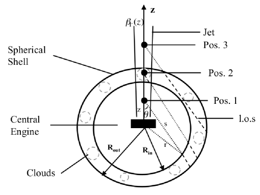
Figure 4: Model for the BLR geometry used in our EC component calculations. The BLR is considered to be a geometrically thick spherical shell that extends from inner, $R_{\rm in,BLR}$, to outer, $R_{\rm out,BLR}$, radius. Three positions of the emission region are marked: (Pos. 1) region is located in the cavity of the BLR, (Pos. 2) region is located within the BLR, and (Pos. 3) region is located outside the BLR. The incoming photon makes an angle $\theta$ with the z-axis (jet axis). Different lines of sight (l.o.s) are shown, which are calculated using the law of cosines between $r,s$ and $\theta$ as described in Appendix A.

The anisotropic profile of emission line intensity obtained using the path length calculations, as described in Appendix A, at the three locations (marked in Figure 4) is shown in Figure 5. The anisotropic intensity due to diffuse BLR emission has a similar profile as that of emission line intensity, and is not shown here for the sake of brevity.

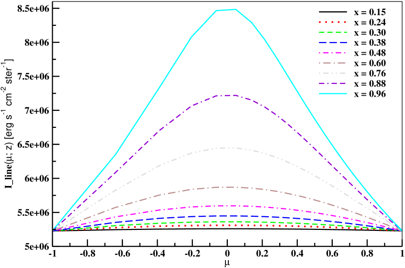
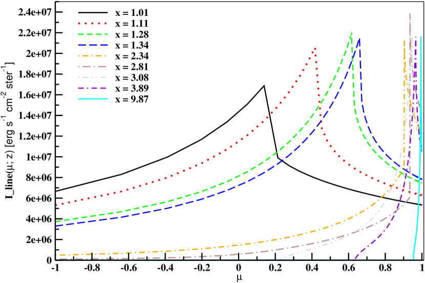
Figure 5: Plot of intensity of radiation as a function of $\mu=\cos{\theta}$, of BLR line emission. The variable $x$ in the figures refers to the distance along the jet axis in units of $R_{\rm in,BLR}$. Input parameters of the base set (see §3) are used to obtain the intensity profile of the BLR emission lines. Left: Intensity profile when the emission region is located at Pos. 1. The profile is symmetric due to equal contribution of all l.o.s from the BLR. The profile peaks as the emission region approaches the inner radius of the BLR at $\sim 0.96R_{\rm in,BLR}$. Right: Intensity profile when the emission region is located at Pos. 2 and 3. The profile becomes asymmetric as the emission region moves to Pos. 2 and Pos. 3 because lines of sight of unequal lengths contribute to the intensity calculation. The intensity distribution peaks at Pos. 2 when the emission region is located within the BLR shell, at $\sim 2.81R_{\rm in,BLR}$ . The intensity plummets as the emission region emerges from the BLR shell, at $\sim 3.08R_{\rm in,BLR}$, and stays constant thereafter.

For the purposes of our study, we consider both the broad line emission and the diffuse continuum radiation to calculate the total radiation field of the BLR. The combined field provides the source of target photons for EC scattering (ECBLR) by jet electrons. The BLR is assumed to emit in the energy range from infrared (IR) to soft X-rays (3 keV), with a characteristic peak frequency of $\nu^{\rm peak}_{\rm BLR}\sim 2\times 10^{15}$  Hz. For the sake of brevity, we drop the subscript $BLR$ from the equations for the rest of this section.

We consider 35 emission lines (34 components from Francis et al. (1991) and the H$\alpha$ component from Gaskell, Shields, & Wampler (1981)) to estimate the total flux of broad emission lines. Using Eq. (19) of Liu & Bai (2006) and Eq. (4), we can obtain the differential line emission photon number density (in $cm^{-3}\epsilon^{-1}ster^{-1}$) in the plasma frame:

$$n^{\prime\rm line}_{\rm ph}(\epsilon^{\prime}_{\rm line},\Omega^{\prime}_{\rm ph};z)=C_{1}\frac{I_{\rm line}(z,\mu)}{\Gamma_{\rm sh}^{4}(1+\beta_{\Gamma_{\rm sh}}\mu^{\prime})^{4}}\frac{N_{\rm V}~{}\delta(\epsilon^{\prime}-\epsilon^{\prime}_{\rm line})}{\epsilon^{\prime}}~{},$$ (15)

where $C_{1}=\frac{1}{m_{e}c^{3}555.77}$, $\epsilon^{\prime}_{\rm line}$ is the dimensionless energy of the incoming photon corresponding to one of the 35 emission line components and $N_{\rm V}$ is the line strength of each of those 35 components, with that of Ly$\alpha$ arbitrarily set at 100 (Francis et al., 1991). We define $\mu^{\prime}$ from $-1$ to $1$ in the plasma frame and use Eq. (2.1) to obtain $\mu$ for the lab frame.

Similarly, using Eqs. (19), (20), and (21) of Liu & Bai (2006) and Eq. (4), we can obtain the differential diffuse continuum photon number density (in $cm^{-3}\epsilon^{-1}ster^{-1}$) in the plasma frame as

$$n^{\prime\rm cont}_{\rm ph}(\epsilon^{\prime}_{\rm cont},\Omega^{\prime}_{\rm ph};z)=C_{2}\frac{I_{\rm cont}(z,\mu)\epsilon^{\prime 2}}{\left(e^{\frac{\epsilon^{\prime}\Gamma_{\rm sh}(1+\beta_{\Gamma_{\rm sh}}\mu^{\prime})}{\Theta}}-1\right)I}~{},$$ (16)

where $C_{2}=\frac{1}{m_{e}c^{3}}$ and $\Theta=1.68\times 10^{-5}$, corresponding to a blackbody temperature of $T=10^{5}$ K, which has been assumed for the inner region of the accretion disk (Liu & Bai, 2006). The quantity $I$ is the total blackbody spectrum, given by

$$I=\int\limits_{\epsilon_{\rm min}}^{\epsilon_{\rm max}}\frac{\epsilon^{3}d\epsilon}{e^{\frac{\epsilon}{\Theta}}-1}~{},$$ (17)

with $\epsilon_{\rm min}=3.22\times 10^{-6}$ corresponding to the photon frequency $\nu_{\rm min}=10^{14.6}$ Hz, and $\epsilon_{\rm max}=2.56\times 10^{-4}$ corresponding to the frequency $\nu_{\rm max}=10^{16.5}$ Hz (Liu & Bai, 2006). Thus, the total anisotropic differential spectral photon number density entering the jet from the BLR is

$$n_{\rm ph}^{\prime}(\epsilon^{\prime},\Omega^{\prime}_{\rm ph})=n^{\prime\rm line}_{\rm ph}(\epsilon^{\prime},\Omega^{\prime}_{\rm ph})+n^{\prime\rm cont}_{\rm ph}(\epsilon^{\prime},\Omega^{\prime}_{\rm ph})~{}.$$ (18)

The electron energy loss rate and photon production rate per unit volume due to ECBLR can be calculated using Eqs. (15), (16) and (18). We use Eq. (6.46) of Dermer & Menon (2009) to obtain the electron energy loss rate in the plasma frame. Substituting Eqs. (6.39) and (6.40) in Eq. (6.46) of Dermer & Menon (2009) yields

$$\dot{\gamma^{\prime}}=\frac{-3c\sigma_{\rm T}}{8}\int\limits_{4\pi}d\Omega^{\prime}_{\rm ph}\int\limits_{0}^{\infty}d\epsilon^{\prime}n_{\rm ph}^{\prime}(\epsilon^{\prime},\Omega^{\prime}_{\rm ph})\{\frac{\ln(D)}{\gamma^{\prime}\epsilon^{\prime}M^{2}}\left[(\gamma^{\prime}-\epsilon^{\prime})(M(M-2)-2)-\gamma^{\prime}\right]+$$

$$\frac{1}{3\epsilon^{\prime}D^{3}}[1-D^{3}+6\epsilon^{\prime}D(\gamma^{\prime}-\epsilon^{\prime})(1+M)(1-\beta_{\gamma^{\prime}}\mu^{\prime})+$$

$$\frac{6D^{2}}{\gamma^{\prime}M}\left(2(\gamma^{\prime}-\epsilon^{\prime})D-\gamma^{\prime}(M(M-1)-1)\right)]\}~{},$$ (19)

where $M=\gamma^{\prime}\epsilon^{\prime}(1-\beta_{\gamma^{\prime}}\mu^{\prime})$ and $D=1+2M$. As can be seen from the above equation, the entire integral is independent of $\phi^{\prime}$ and can be solved analytically. Similarly, after substituting Eqs. (15) and (16) in Eq. (2.2), the $d\epsilon^{\prime}$ integral can be solved analytically for $n^{\prime\rm line}_{\rm ph}(\epsilon^{\prime},\Omega^{\prime}_{\rm ph})$ due to the presence of the $\delta(\epsilon^{\prime}-\epsilon^{\prime}_{\rm line})$ function in its expression (see Eq. 15). After having carried out these simplifications, Eq. (2.2) is solved numerically to obtain the final electron energy loss rate due to the ECBLR process.

In the case that all scattering occurs in the Thomson regime, $\gamma^{\prime}\epsilon^{\prime}\ll 1$, the electron energy loss rate can be directly calculated by substituting $\langle\epsilon_{S}^{0}\sigma\rangle=\sigma_{T}$ and $\langle\epsilon_{S}^{1}\sigma\rangle=\sigma_{T}\gamma^{\prime 2}\epsilon^{\prime}(1-\cos\psi^{\prime})$ into Eq. (6.46) of Dermer & Menon (2009). After carrying out integrations over $d\phi^{\prime}$ and $d\epsilon^{\prime}$ analytically for both $n^{\prime\rm line}_{\rm ph}(\epsilon^{\prime},\Omega^{\prime}_{\rm ph})$ and $n^{\prime\rm cont}_{\rm ph}(\epsilon^{\prime},\Omega^{\prime}_{\rm ph})$, the Thomson-regime electron energy loss rate expression for the ECBLR process is given by

$$\dot{\gamma^{\prime}}=-2\pi c\sigma_{\rm T}C_{2}\int\limits_{-1}^{1}d\mu^{\prime}\frac{(1-\beta_{\gamma^{\prime}}\mu^{\prime})(\gamma^{\prime 2}(1-\beta_{\gamma^{\prime}}\mu^{\prime})-1)}{\Gamma_{\rm sh}^{4}\left(1+\beta_{\Gamma_{\rm sh}}\mu^{\prime}\right)^{4}}\left[I_{\rm line}(z,\mu)+\frac{\left(\pi\Theta\right)^{4}}{15I}I_{\rm cont}(z,\mu)\right]~{}.$$ (20)

Here, we have used the result $\int\limits_{0}^{\infty}dx\frac{x^{3}}{e^{xa}-1}=\frac{\pi^{4}}{15a^{4}}$. As can be seen from Fig. 3, the Thomson approximation for ECBLR deviates from the corresponding full expression at $\gamma^{\prime}\geq 100$.

The ECBLR photon production rate per unit volume, under the head-on approximation, is calculated using Eq. (6.32) of Dermer & Menon (2009). We write it in terms of the differential photon production rate using Eq. (2.1), and substitute the expression for the differential photon number density of BLR photons from Eq. (18) to obtain

$$\dot{n^{\prime}}(\epsilon_{s}^{\prime},\Omega_{s}^{\prime})=\frac{3c\sigma_{T}}{32\pi}\int\limits_{0}^{2\pi}d\phi^{\prime}_{\rm ph}\int\limits_{-1}^{1}d\mu^{\prime}\int\limits_{0}^{\epsilon^{\prime}_{\rm max}}d\epsilon^{\prime}\frac{n_{\rm ph}^{\prime}(\epsilon^{\prime},\Omega^{\prime}_{\rm ph})}{\epsilon^{\prime}}\\ \int\limits_{\gamma^{\prime}_{\rm low}}^{\infty}d\gamma^{\prime}\frac{n^{\prime}_{e}(\gamma^{\prime})}{\gamma^{{}^{\prime}2}}\Xi_{\rm C}~{},$$

where the quantities used in the above equation have been explained in §2.1. As mentioned in §2.1, the Compton cross-section in the above expression is evaluated such that in the case of scatterings for which $\gamma^{\prime}\epsilon^{\prime}<0.1$, we use Eq. (44) of Dermer et al. (2009) to calculate it in the Thomson regime, under head-on approximation.

For cases where all scattering occurs in the Thomson regime, Eqs. (12) and (13) yield

$$\dot{n}^{\prime\rm Th}(\epsilon^{\prime}_{\rm S},\Omega^{\prime}_{\rm S})=\frac{c\sigma_{\rm T}}{4\pi}\int\limits_{4\pi}d\Omega^{\prime}_{\rm ph}\int\limits_{1}^{\infty}d\gamma^{\prime}n^{\prime}_{e}(\gamma^{\prime})(1-\beta_{\gamma^{\prime}}\cos\psi^{\prime})\int\limits_{0}^{\infty}d\epsilon^{\prime}n^{\prime}_{\rm ph}(\epsilon^{\prime},\Omega^{\prime}_{\rm ph})$$

$$\delta\left(\epsilon^{\prime}_{\rm S}-\gamma^{\prime 2}\epsilon^{\prime}\left[1-\beta_{\gamma^{\prime}}\cos\psi^{\prime}\right]\right)~{}.$$ (21)

Solving for $d\epsilon^{\prime}$ analytically, we obtain the Thomson regime photon production rate per unit volume as

$$\dot{n}^{\prime\rm Th}(\epsilon^{\prime}_{\rm S},\Omega^{\prime}_{\rm S})=\frac{c\sigma_{\rm T}}{4\pi}\int\limits_{4\pi}d\Omega^{\prime}_{\rm ph}\int\limits_{1}^{\infty}d\gamma^{\prime}\frac{n^{\prime}_{e}(\gamma^{\prime})}{\gamma^{\prime 2}}n^{\prime}_{\rm ph}\left(\frac{\epsilon^{\prime}_{\rm S}}{\gamma^{\prime 2}(1-\beta_{\gamma^{\prime}}\cos\psi^{\prime})},\Omega^{\prime}_{\rm ph}\right)~{}.$$ (22)

Now substituting Eqs. (15) and (16) in Eq. (22) and solving for the delta function (present in Eq. (15)) in the $d\gamma^{\prime}$ integral for the line emission part, we can obtain the final expression for the ECBLR Thomson-regime photon production rate per unit volume as

$$\dot{n}^{\prime\rm Th}(\epsilon^{\prime}_{\rm S},\Omega^{\prime}_{\rm S})=\frac{c\sigma_{\rm T}}{4\pi}\int\limits_{4\pi}d\Omega^{\prime}_{\rm ph}[\frac{C_{1}}{2}\frac{I_{\rm line}(z,\mu)}{\Gamma_{\rm sh}^{4}\left(1+\beta_{\Gamma_{\rm sh}}\mu^{\prime}\right)^{4}}\sqrt{\frac{1-\cos\psi^{\prime}}{\epsilon^{\prime}_{\rm S}}}\sum_{\epsilon^{\prime}_{\rm line}}\frac{N_{\rm V}}{\epsilon^{\prime 3/2}_{\rm line}}n_{e}\left(\sqrt{\frac{\epsilon^{\prime}_{\rm S}}{\epsilon^{\prime}_{\rm line}(1-\cos\psi^{\prime})}}\right)$$

$$+C_{2}\frac{I_{\rm cont}(z,\mu)\epsilon^{\prime 2}_{\rm S}}{I}\int\limits_{1}^{\infty}d\gamma^{\prime}\frac{n^{\prime}_{e}(\gamma^{\prime})}{\gamma^{\prime 6}\left(1-\beta_{\gamma^{\prime}}\cos\psi^{\prime}\right)^{2}}\left(e^{\frac{\epsilon^{\prime}_{\rm S}\Gamma_{\rm sh}(1+\beta_{\Gamma_{\rm sh}}\mu^{\prime})}{\gamma^{\prime 2}(1-\beta_{\gamma^{\prime}}\cos\psi^{\prime})\Theta}}-1\right)^{-1}]~{}.$$ (23)

Where we evaluate the line emission term of the above equation for cases where $\gamma^{\prime}\geq 10$ so that $\beta_{\gamma^{\prime}}\simeq 1$ and the $d\gamma^{\prime}$ integral can be solved analytically using the delta function that is present in the expression for the differential line emission photon number density.

2.3 The Dusty Torus

We consider a clumpy molecular torus (Sokolov & Marscher, 2005; Marscher, 2013) whose emission is dominated by dust and which radiates as a blackbody at IR frequencies at a temperature T = 1200 K (Malmrose et al., 2011) in the lab frame. The torus lies in the plane of the accretion disk and extends from $R_{\rm in,DT}$ to $R_{\rm out,DT}$. As shown in Fig. 6, the central circle of the torus is located at a distance of $r_{\rm DT}=\frac{R_{\rm out,DT}+R_{\rm in,DT}}{2}$ from the central source and the cross-sectional radius of the torus is given by $R_{\rm T}=\frac{R_{\rm out,DT}-R_{\rm in,DT}}{2}$. We assume that the incident radiation comes from a portion of the inner surface of the torus. This portion, which is the covering factor, is dependent on the size of the torus.

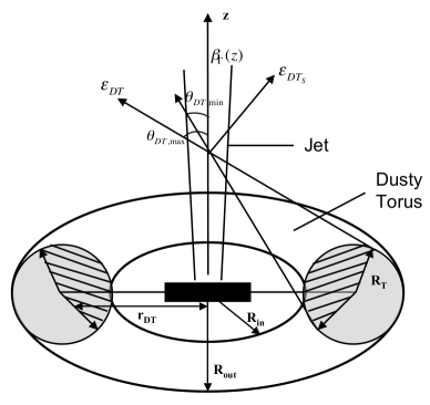
Figure 6: Model for the DT geometry used in our EC component calculations. The DT is considered to be a patchy molecular torus that extends from inner, $R_{\rm in,DT}$, to outer, $R_{\rm out,DT}$ radius. The central circle of the torus is located at a distance $r_{\rm DT}$ from the central engine. The shaded portion shows the cross-sectional area of the torus with radius $R_{\rm T}$. Only a fraction of the torus facing the central continuum source (cross-hatched region) is assumed to be hot enough to be visible to the emission region on the z-axis. Incoming photons from this portion of the surface enter the jet at angles whose range is governed by a minimum, $\theta_{\rm DT,min}$, and a maximum, $\theta_{\rm DT,max}$. The dimensionless energy of an incoming photon is given by $\epsilon_{\rm DT}$, while that of the scattered or the outgoing photon is given by $\epsilon_{\rm DT,S}$.

The DT is assumed to emit IR photons with a characteristic peak frequency of the radiation field, $\nu^{\rm peak}_{\rm DT}\sim 3\times 10^{13}$  Hz. For the sake of brevity, we drop the subscript $DT$ from all quantities listed in this section. The minimum, $\theta_{\rm min}$, and maximun, $\theta_{\rm max}$, incident angles constraining the incident emission from the torus are given by

$$\theta_{\rm min}=\sin^{-1}{\frac{r}{\sqrt{z^{2}+r^{2}}}}-\sin^{-1}{\frac{R_{\rm T}}{\sqrt{z^{2}+r^{2}}}}$$

$$\theta_{\rm max}=\sin^{-1}{\frac{r}{\sqrt{z^{2}+r^{2}}}}+\sin^{-1}{\frac{R_{\rm T}}{\sqrt{z^{2}+r^{2}}}}~{}.$$ (24)

These angles are subsequently transformed into the plasma frame according to:

$$\eta^{\prime}=\cos{\theta^{\prime}}=\frac{\cos{\theta}-\beta_{\Gamma_{\rm sh}}}{1-\beta_{\Gamma_{\rm sh}}\cos{\theta}}~{}.$$ (25)

The covering factor of the dusty torus, $f_{\rm cov}$, can be obtained in terms of the fraction, $\xi$, of the disk luminosity, $L_{\rm disk}$, that illuminates the torus such that, $L_{\rm Dust}=\xi L_{\rm disk}$. Here we take $\xi=0.22$ as found for PKS 1222+216 by Malmrose et al. (2011). Also, the following relationship holds between $L_{\rm Dust}$, $f_{\rm cov}$, and the illuminated area of the torus, $A_{\rm obs}$:

$$L_{\rm Dust}=A_{\rm obs}\sigma_{\rm SB}T^{4}f_{\rm cov}~{},$$ (26)

The illuminated area of the torus visible from a position in the jet is given by

$$A_{\rm obs}\approx\frac{\pi^{2}}{4}(R_{\rm out}^{2}-R_{\rm in}^{2})~{},$$ (27)

where the factor of 1/4 appears because only the front side of the inner torus is illuminated and only half of this is visible to the emitting region in the lab frame. Thus, for given values of $R_{\rm in}$, $R_{\rm out}$, and $L_{\rm disk}$, the covering factor of the torus can be obtained from Eqs. (26) and (27). Conversely, for given values of $f_{\rm cov}$ and $R_{\rm in}$, we can also obtain the extent of the torus in terms of $R_{\rm out}$ and the corresponding values of $r$ and $R_{\rm T}$.

Since the torus emits as a blackbody, the differential spectral photon number density in the plasma frame is simply given by

$$n^{\prime}_{\rm ph}(\epsilon^{\prime},\Omega^{\prime}_{\rm ph})=2\left(\frac{m_{e}c}{h}\right)^{3}f_{\rm cov}\frac{\epsilon^{\prime 2}}{e^{\frac{\epsilon^{\prime}\Gamma_{\rm sh}(1+\beta_{\Gamma_{\rm sh}}\eta^{\prime})}{\Theta}}-1}~{},$$ (28)

where we have used Eq. (4) to convert the differential photon density from the lab to the plasma frame. Fig. 7 shows the anisotropic intensity profile of the DT as a function of incident angle, $\mu^{\prime}=\cos{\theta^{\prime}}$, in the plasma frame.

Figure 7: Plot of intensity of radiation from the DT as a function of distance, $z$, along the jet axis and the incident angle of incoming photons $\mu^{\prime}=\cos{\theta^{\prime}}$. The variable $x$ in the figure refers to the value of $z$ in terms of $R_{\rm in,BLR}$. Input parameters of the base set (see §3) have been used to obtain the anisotropic intensity profile of the DT emission. Since only a fraction of the torus emits radiation in the direction of the emission region, at smaller values of $z$, incoming photons enter the jet from the front but cover a very narrow range of angles. As the emission region moves outward along the jet axis (e.g., $z=6.20R_{\rm inBLR}$), incoming photons from the DT cover a broader range of angles but enter the jet more from the side, which leads to de-boosting and reduces the overall intensity of radiation in the plasma frame. The dotted lines in the figure indicate the range of angles that contribute to the DT intensity at that distance; beyond this range the intensity drops to zero.

We substitute Eq. (28) in Eq. (2.2) to calculate the electron energy loss rate due to ECDT, which yields

$$\dot{\gamma^{\prime}}=\frac{-3c\pi\sigma_{\rm T}}{2}\left(\frac{m_{e}c}{h}\right)^{3}f_{\rm cov}\int\limits_{\eta^{\prime}_{\rm min}}^{\eta^{\prime}_{\rm max}}d\eta^{\prime}\int\limits_{0}^{\infty}d\epsilon^{\prime}\frac{\epsilon^{\prime 2}}{e^{\frac{\epsilon^{\prime}\Gamma^{\rm sh}(1+\beta_{\Gamma_{\rm sh}}\eta^{\prime})}{\Theta}}-1}\{\frac{\ln(D)}{\gamma^{\prime}\epsilon^{\prime}M^{2}}\left[(\gamma^{\prime}-\epsilon^{\prime})(M(M-2)-2)-\gamma^{\prime}\right]$$

$$+\frac{1}{3\epsilon^{\prime}D^{3}}[1-D^{3}+6\epsilon^{\prime}D(\gamma^{\prime}-\epsilon^{\prime})(1+M)(1-\beta_{\gamma^{\prime}}\eta^{\prime})+$$

$$\frac{6D^{2}}{\gamma^{\prime}M}\left(2(\gamma^{\prime}-\epsilon^{\prime})D-\gamma^{\prime}(M(M-1)-1)\right)]\}.$$ (29)

For cases where all scattering occurs in the Thomson regime, we follow the steps described in §2.2 to obtain Eq. (20), which yields the Thomson-regime electron energy loss rate for the ECDT process as

$$\dot{\gamma^{\prime}}=\frac{-4\pi^{5}c\sigma_{\rm T}\Theta^{4}}{15\Gamma_{\rm sh}^{4}}\left(\frac{m_{e}c}{h}\right)^{3}f_{\rm cov}\int\limits_{\eta^{\prime}_{\rm min}}^{\eta^{\prime}_{\rm max}}d\eta^{\prime}\frac{(1-\beta_{\gamma^{\prime}}\eta^{\prime})\left[\gamma^{\prime 2}(1-\beta_{\gamma^{\prime}}\eta^{\prime})-1\right]}{\left(1+\beta_{\Gamma_{\rm sh}}\eta^{\prime}\right)^{4}}~{}.$$ (30)

As shown in Fig. 3, the Thomson approximation for ECDT deviates from the corresponding full expression above $\gamma^{\prime}\sim 3\times 10^{3}$. We substitute Eq. (28) in Eq. (2.2) to obtain the ECDT photon production rate per unit volume, under the head-on approximation, as

$$\dot{n^{\prime}}(\epsilon_{s}^{\prime},\Omega_{s}^{\prime})=\frac{3c\sigma_{\rm T}}{16\pi}\left(\frac{m_{e}c}{h}\right)^{3}f_{\rm cov}\int\limits_{0}^{2\pi}d\phi^{\prime}_{\rm ph}\int\limits_{\eta^{\prime}_{\rm min}}^{\eta^{\prime}_{\rm max}}d\eta^{\prime}\int\limits_{0}^{\epsilon^{\prime}_{\rm max}}d\epsilon^{\prime}\frac{\epsilon^{\prime}}{e^{\frac{\epsilon^{\prime}\Gamma_{\rm sh}(1+\beta_{\Gamma_{\rm sh}}\eta^{\prime})}{\Theta}}-1}\\ \int\limits_{\gamma^{\prime}_{\rm low}}^{\infty}d\gamma^{\prime}\frac{n^{\prime}_{e}(\gamma^{\prime})}{\gamma^{{}^{\prime}2}}\Xi_{\rm C}~{}.$$

For scatterings occuring entirely in the Thomson regime, we substitute Eq. (28) in Eq. (2.2) to obtain the ECDT Thomson-regime photon production rate per unit volume,

$$\dot{n}^{\prime\rm Th}(\epsilon^{\prime}_{\rm S},\Omega^{\prime}_{\rm S})=\frac{c\sigma_{\rm T}}{2\pi}\left(\frac{m_{e}c}{h}\right)^{3}f_{\rm cov}\int\limits_{0}^{2\pi}d\phi^{\prime}\int\limits_{\eta^{\prime}_{\rm min}}^{\eta^{\prime}_{\rm max}}d\eta^{\prime}\int\limits_{1}^{\infty}d\gamma^{\prime}\frac{n^{\prime}_{e}(\gamma^{\prime})}{\gamma^{\prime 6}\left(1-\beta_{\gamma^{\prime}}\cos{\psi^{\prime}}\right)^{2}}\left[e^{\frac{\epsilon^{\prime}_{\rm S}\Gamma_{\rm sh}(1+\beta_{\Gamma_{\rm sh}}\eta^{\prime})}{\Theta\gamma^{\prime 2}(1-\beta_{\gamma^{\prime}}\cos{\psi^{\prime}})}}-1\right]^{-1}~{}.$$ (31)

3 Parameter Study and Results

We explore the effects of varying the contribution of the disk, the BLR, and the DT on the resultant seed photon fields and their manifestation on the simulated SED and lightcurves of a typical blazar. This is important for understanding the evolution of the HE emission of blazars as a function of distance down the jet and thus gain insight on the location of the observed $\gamma$-ray emission.

3.1 Our Baseline Model

For the purposes of this study, the flux values are calculated for the frequency range $\nu^{\prime}=(10^{8}-10^{26})$ Hz and for the electron energy distribution (EED) range $\gamma^{\prime}=10-10^{8}$, with both ranges divided into 50 grid points. The entire emission region is divided into 100 slices with 50 slices in the forward and 50 in the reverse shock regions. The code has been fully parallelized using the OpenMP interface. This has resulted in significant speed-up in the time-dependent numerical calculation of radiative transfer processes in our multi-zone scenario.

Table 1 shows the values of the base set (run 1) parameters used to obtain our baseline model. The parameters of this generic blazar are motivated by a fit to the blazar 3C 279 for modeling rapid variability on timescales of $\sim$ 1 day. The input parameters up to $\theta^{*}_{\rm obs}$ have been explained in Paper 1, except for $z_{i}$ and $z_{o}$, which refer to the location of inner and outer shells, respectively, along the jet axis. These values are used to calculate the point of collision, $z_{c}$, along the z axis (see Paper 1 for details), which determines the initial location of the emission region along the jet axis. According to the model description given in Paper I, the input parameters for the base set are used to obtain a value for the BLF of the emission region, which in this case is $\Gamma_{\rm sh}=14.9$. The BLF value in turn yields a magnetic field strength of $B^{\prime}=2.71$ G and $\gamma^{\prime}_{\rm max}=1.26\times 10^{5}$ for both the forward and reverse emission regions. On the other hand, the value of $\gamma^{\prime}_{\rm min}$ is numerically obtained to be $8.81\times 10^{2}$ for the forward and $1.85\times 10^{3}$ for the reverse emission regions. Similarly, the total widths of the forward and reverse emission regions are analytically obtained to be $\Delta^{\prime}_{\rm fs}=1.01\times 10^{16}$ cm and $\Delta^{\prime}_{\rm rs}=2.12\times 10^{16}$ cm, respectively, which consequently yields a shock crossing time for each of the emission regions of $t^{\prime}_{\rm cr,fs}=8.93\times 10^{5}$ s and $t^{\prime}_{\rm cr,rs}=1.37\times 10^{6}$ s. In the observer’s frame, this corresponds to the forward shock (FS) spending $\sim 15$ hours in the forward emission region and the reverse shock (RS) spending $\sim 23$ hours in the reverse emission region. The width, and consequently shock crossing time, for each of the emission regions is set such that it is comparable to the flaring period of our simulation.

The inner and outer shells collide at a distance of $z_{c}=1.01\times 10^{17}$ cm, making this the starting position of the emission region along the jet axis. The entire simulation runs for a total of $\sim 5$ days in the observer’s frame, during which the emission region moves beyond the BLR and into the DT, covering a distance of 1.04 pc, in the AGN frame. For our baseline model, the forward shock exits the forward emission region within a day in the observer’s frame, when the emission region is located in the cavity of the BLR at $\sim 0.16$ pc. Similarly, the reverse shock exits its region within a day when the emission region is located within the BLR at $\sim 0.24$ pc. Over the time scale of our simulation, the BLR energy density, $u^{\prime}_{\rm ph,BLR}$, changes from $2.82\times 10^{-2}$ to $1.18\times 10^{-5}~{}erg~{}cm^{-3}$, while the DT energy density, $u^{\prime}_{\rm ph,DT}$, evolves from $3.62\times 10^{-2}$ to $5.62\times 10^{-3}~{}erg~{}cm^{-3}$.

Table 1: Parameter list of run 1 used to obtain the baseline model.

Parameter	Symbol	Value
Kinetic Luminosity	$L_{w}$	$5\times 10^{47}$ erg/s
Event Duration	$t_{w}$	$10^{7}$ s
Outer Shell Mass	$M_{o}$	$1.531\times 10^{32}$ g
Inner Shell BLF	$\Gamma_{i}$	26.3
Outer Shell BLF	$\Gamma_{o}$	10
Inner Shell Width	$\Delta_{i}$	$6.2\times 10^{15}$ cm
Outer Shell Width	$\Delta_{o}$	$7.4\times 10^{15}$ cm
Inner Shell Position	$z_{i}$	$7.8\times 10^{15}$ cm
Outer Shell Position	$z_{o}$	$1.56\times 10^{16}$ cm
Electron Energy Equipartition Parameter	$\varepsilon^{\prime}_{e}$	$9\times 10^{-2}$
Magnetic Energy Equipartition Parameter	$\varepsilon^{\prime}_{B}$	$2.5\times 10^{-3}$
Fraction of Accelerated Electrons	$\zeta^{\prime}_{e}$	$1\times 10^{-2}$
Acceleration Timescale Parameter	$\alpha^{\prime}$	$2\times 10^{-5}$
Particle Injection Index	$q^{\prime}$	4.0
Slice/Jet Radius	$R^{\prime}_{z}$	$5.44\times 10^{16}$ cm
Observer Frame Observing Angle	$\theta^{*}_{\rm obs}$	$1.5\deg$
Disk Luminosity	$L_{\rm disk}$	$8\times 10^{45}$ erg/s
BH Mass	$M_{\rm BH}$	$2\times 10^{8}M_{\odot}$
Accretion Efficiency	$\eta_{\rm acc}$	0.06
BLR Luminosity	$L_{\rm BLR}$	$8\times 10^{44}$ erg/s
BLR inner radius	$R_{\rm in,BLR}$	$6.17\times 10^{17}$ cm
BLR outer radius	$R_{\rm out,BLR}$	$1.85\times 10^{18}$ cm
BLR optical depth	$\tau_{\rm BLR}$	0.01
BLR covering factor	$f_{\rm cov,BLR}$	0.03
DT inner radius	$R_{\rm in,DT}$	$3.086\times 10^{18}$ cm
DT outer radius	$R_{\rm out,DT}$	$6.17\times 10^{18}$ cm
Ldisk fraction	$\xi$	0.2
DT covering factor	$f_{\rm cov,DT}$	0.2
Redshift	$Z^{*}$	0.538

Figure 8 shows the instantaneous broadband spectra and the time-averaged SED from the baseline model. Since we are focussing on rapid variability in this study, we have evaluated the SED averaged over an integration time of $\sim$ 1 day. As mentioned in Paper 1, each instantaneous spectrum shown in Fig. 8 corresponds to a combination of multiple instantaneous SEDs, from both forward and reverse emission regions, binned over a time period of 9 ks. This was done to facilitate file management on the computational facility being used and to be able to compare instantaneous SEDs to X-ray observations, which have a typical integration time of the same order. The time-averaged SED is shown by the heavy solid curve on the left side of Fig. 8, while the right side illustrates time-averaged radiative components responsible for the total time-averaged SED. In our framework, although the time-averaged components dictate the overall profile of the SED and clearly show which component is responsible for emission in a particular energy band, they do not exactly match the level of the total time-averaged SED. This is because, in our model, individual radiative components are calculated from the emission coefficients rather than from the actual escaping radiative flux.

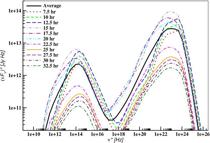
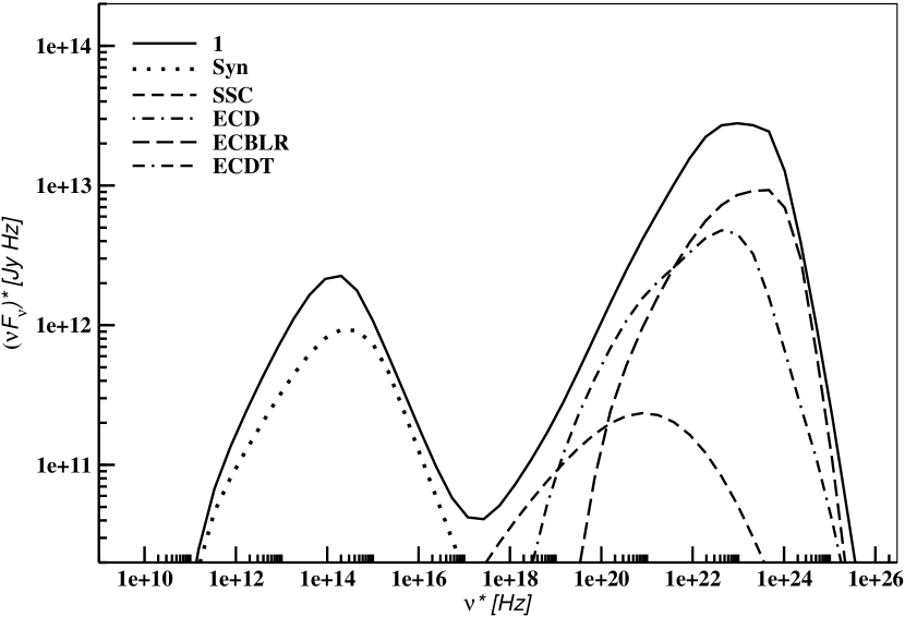
Figure 8: Sample SEDs from the computations. Left: Simulated instantaneous spectra of the baseline model of a generic blazar. The thick solid black line shows the SED resulting from averaging over an integration period of 1 day, corresponding to a rapid flare of that duration. The SEDs corresponding to 9 ks and 18 ks have not been considered in time-averaging since they correspond to a state when the system is still chaotic as it gradually approaches equilibrium. Right: Time-averaged SED showing individual radiation components as dotted: synchrotron; small-dashed: SSC; dot-dashed: ECD, which cannot be seen since its contribution is below $10^{10}$ Jy Hz for this case; long-dashed: ECBLR; and dot-double dash: ECDT.

The instantaneous SEDs shown in the left hand side of Fig. 8 exhibit the effects of acceleration and cooling on the broadband spectra of our generic blazar in a time-dependent manner. As the shocks propagate through the system and energize an increasingly larger volume of the emitting regions, the overall flux level of the spectra continues to increase without affecting the location of peak frequencies for the synchrotron and EC component. Once the emission from the system reaches its maximum (at $\sim$ 15 hr in this case), by which time the forward shock has already left the forward emission region, cooling starts to show its effects on the SEDs, with the entire broadband spectrum extending to progressively lower frequencies and the overall flux declining steadily. At later times ($\sim$ 17.5 hr onwards), the emission comes from a comparatively smaller volume of the emitting region, with the reverse emission region contributing the most at this time since the reverse shock is still present in the system. This implies that fresh high-energy electrons, which dominate the emission at the synchrotron peak, are still being injected into the system at that time. Consequently, the synchrotron component after 17.5 hr does not progress to lower frequencies, although the high-energy component does.

As can be seen from the right side of Fig. 8, the EC component peaks in the $\gamma$-ray regime at $\sim 10\times 10^{23}$ Hz, while the synchrotron component peaks in the near-IR at $\sim 2\times 10^{14}$ Hz. The transition from synchrotron to high-energy emission takes place in the X-ray range at $\sim 3\times 10^{17}$ Hz. As can be seen from Fig. 8, the EC emission of the base set is dominated by the ECBLR component, which peaks at $\sim 0.4$ GeV. For the flux level (in Jy Hz) considered for our cases, the ECD component does not contribute to the HE component of this blazar, while the ECDT component is responsible for the emission in the MeV range reaching its maximum level at $\sim 200$ MeV. As a result, ECBLR and ECDT are the two major components that govern the cooling of electrons/positrons due to EC emission. The derived Compton dominance factor (CDF), defined as CDF = $\nu F^{*~{}\rm EC,peak}_{\nu}/\nu F^{*~{}\rm syn,peak}_{\nu}$, is 12.4. The spectral hardness (SH) of the SED can be quantified in terms of the photon spectral index, which is found to be $\alpha^{*}_{\rm 2-10keV}=0.59$ in the X-ray (2 - 10 keV) range and is indicative of a hard SSC-dominated X-ray spectrum. The Fermi range photon spectral index (calculated at 10 GeV) is $\alpha^{*}_{\rm 10GeV}=2.75$ and implies a much softer $\gamma$-ray spectrum. The left side of Fig. 9 shows a comparison of total energy density, $u^{\prime}_{\rm ph}$ (in units of $erg~{}cm^{-3}$) due to the BLR and DT photon fields for our baseline model. As can be seen, energy densities due to the two photon fields are comparable to each other at sub-pc scales, with the BLR energy density peaking at $\sim$ 0.21 pc and plummeting beyond this. The DT energy density takes over at $\sim 0.3$ pc and remains the dominant contributor to the seed photon field out to $\sim$ 3 pc. The long-dashed curve in the figure shows a more accurate representation of the BLR energy density, which was obtained by using a linear grid for $\mu^{\prime}_{\rm ph,BLR}$ consisting of 4000 points. In order to save computation time in calculating intensities due to BLR line and diffuse continuum emission at each of these points, we switched to the Gaussian quadrature method for evaluating integrals over BLR angles. The Gaussian grid consisted of only 48 points and resulted in faster calculations. The percent difference between these two approaches is 27% in the beginning, reducing to 12% at the peak of the BLR energy density profile. The initial difference of 27% is not expected to change or affect our inferences on the dominance of a particular EC process on the overall profile of SEDs, because this difference is overshadowed by the amount of boosting BLR photons receive while entering the jet from the front.

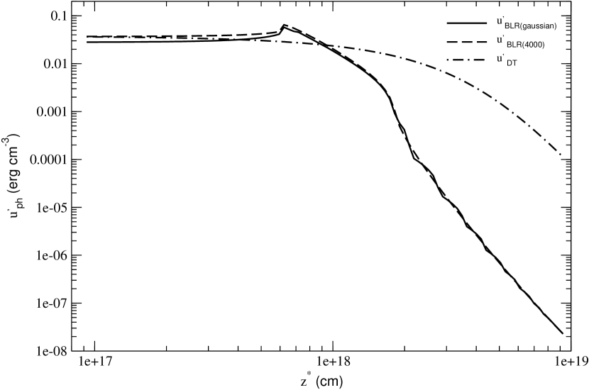
Figure 9: Energy density profiles of BLR and DT photon fields for the baseline model. The black solid curve denotes BLR energy density profile calculated using a Gaussian quadrature method for evaluating integrals over BLR angles. The long-dashed curve represents the same as mentioned above, but using a linear grid for BLR angles consisting of 4000 points. The percent difference between the two approaches is 27%. The dot-dashed curve illustrates the DT energy density profile out to a distance of $\sim$ 3 pc.

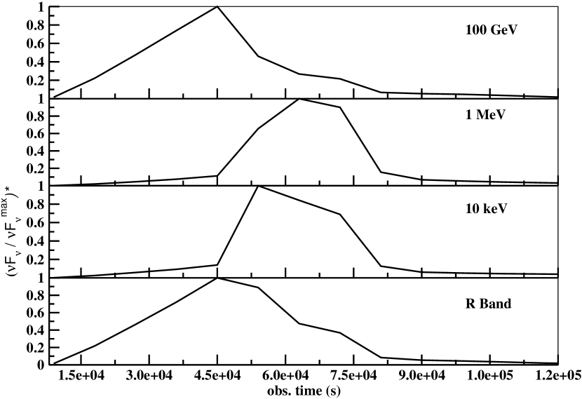
Figure 10: Simulated light curves at R band, 10 keV, 1 MeV, and 100 GeV energies resulting from our baseline model with parameters listed in Table 1.

Figure 10 shows light curves in the optical (R band), X-ray (10 keV), HE $\gamma$-ray (1 MeV), and $\gamma$-ray in the upper Fermi range (100 GeV) spectral regimes from our baseline model for a 1-day flaring period. As can be seen from the figure, the synchrotron-dominated optical and EC-dominated HE emission in the 100 GeV energy range are governed by the presence of shocks in the system. As explained in Paper 1, the respective pulses steadily rise for as long as the acceleration of particles operates and both reach their maximum at $t^{*}_{\rm peak}$ = 45 ks, after which they start to decline rapidly. The Fermi light curve starts to decline sooner and decays faster than the R-band light curve as long as the FS is present in the system (until $t^{*}_{\rm FS,exit}\sim$ 53 ks). Once the FS exits, the Fermi light curve becomes shallower, while the R-band light curve undergoes a sharper decline, which is marked by a break in the decaying part of the respective pulse profiles. This is because, as also mentioned in Paper 1, higher energy electrons are involved in producing optical synchrotron and 100 GeV EC photons. Such electrons cool on a timescale shorter than the dynamical timescale within a particular zone. Thus, once the shocks exit their respective emission regions and radiative cooling prevails in that region, the optical and 100 GeV pulse rapidly decay. This makes the rising and decaying phases of the pulse nearly equal and result in a quasi-symmetrical pulse profile. The X-ray light curve at 10 keV is a result of upscattering of lower energy (near IR) synchrotron photons by lower energy electrons and is dominated by the low-energy end of SSC emission. Since such electrons remain in the system for an extended period of time, the X-ray light curve peaks later than the optical and Fermi light curves. At the same time, there is a continued build-up of late-arriving photons at scattering sites, due to which the pulse peaks later and exhibits a much more gradual decline, resulting in an asymmetrical pulse profile (Joshi & Böttcher, 2011). The 1 MeV light curve, on the other hand, results from the rising part of the ECDT emission, with some contribution from that of the ECBLR component. This implies that lower energy electrons are responsible for emission in this energy range compared to those responsible for the optical and 100 GeV emission. As a result, the 1 MeV flux is last to peak at $t^{*}_{\rm peak}$ = 63 ks. Since the timescale of decay is inversely proporational to the characteristic energy of the electrons responsible for the respective emission, the 1 MeV light curve decays later compared to its 100 GeV counterpart.

3.2 Parameter Variation

Here, we explore the effects of varying physical parameters related to the EC emission in order to understand their impact on the evolution of broadband spectra and light curves of our generic blazar. For all the cases described below, the simulation run time is the same as that of the baseline model, which is $\sim$ 5 days in the observer’s frame. Table 2 shows the values of each of the parameters that are varied in the rest of the simulations. We describe the effects of varying these parameters on the time-averaged SEDs and light curves with respect to that of the baseline model in sections 3.2.1 - 3.2.3.

Table 2: Parameter list for other simulations. The corresponding values of the baseline model are also listed here for reference.

Run #	Parameter Value	Baseline Model
2	$z_{c}=0.05~{}R_{\rm in,BLR}$	$0.16~{}R_{\rm in,BLR}$
3	$z_{c}=0.81~{}R_{\rm in,BLR}$
4	$z_{c}=3.10~{}R_{\rm in,BLR}$
5	$L_{\rm BLR}=8\times 10^{43}erg~{}s^{-1}$	$8\times 10^{44}erg~{}s^{-1}$
6	$L_{\rm BLR}=7.2\times 10^{45}erg~{}s^{-1}$
7	$f_{\rm cov,DT}=0.01$	0.2
8	$f_{\rm cov,DT}=0.9$

3.2.1 Variations of $z_{c}$

Figure 11 shows the impact of changing the starting position along the jet axis, $z_{c}$, of the emission region on the time-averaged SEDs and light curves of our baseline model. As described in §3.1, the point of collision decides the starting position of the emission region along the z-axis. Changing this location and understanding its effect on the resultant SED and light curves is important in comprehending the effect of the AGN environment as the emission region moves spatially through it.

In the case of run 2, the starting position of the emission region is at $z_{c}=3.08\times 10^{16}$ cm or $\sim 5\times 10^{-2}~{}R_{\rm in,BLR}$. During this run, the emission region moves beyond the BLR, covering a distance of 1.02 pc, in the AGN frame, similar to that of run 1. In this case, the FS exits the system when the emission region is located in the cavity of the BLR, but closer to the central engine compared to that of run 1, at $z\sim 0.14$ pc or $\sim 0.7~{}R_{\rm in,BLR}$. The RS exits the system when the emission region is located within the BLR at $z\sim 0.21$ pc or $\sim 1.1~{}R_{\rm in,BLR}$. In the case of run 3, $z_{c}=5.02\times 10^{17}cm$ or $\sim 0.8~{}R_{\rm in,BLR}$. Here, the emission region moves slightly deeper into the DT compared to that of run 1, and ends at a distance of 1.17 pc. In this case the FS exits the system when the emission region is located within the BLR at $z\sim 0.29$ pc or $\sim 1.5~{}R_{\rm in,BLR}$ and the RS exits the system when the region is at $z\sim 0.36$ pc or $\sim 1.8~{}R_{\rm in,BLR}$. In the case of run 4, the emission region is placed beyond the BLR at $z_{c}=1.91\times 10^{18}$ cm or $\sim 3~{}R_{\rm in,BLR}$. Consequently, the system evolves until 1.63 pc with the FS exiting the system at $z\sim 0.75$ pc or $\sim 3.7~{}R_{\rm in,BLR}$ and the RS at $z\sim 0.82$ pc or $\sim 4.1~{}R_{\rm in,BLR}$.

As can be seen from the left side of Fig. 11, placing the emission region closer to the central engine (run 2) or closer to the inner radius of the BLR (run 3) doesn’t change the overall profile of the time-averaged SED. This is because, just like run 1, in both cases the high-energy emission continues to be dominated by the ECBLR process. In other words, the total external radiation energy density, as received by the emission region in its comoving frame, does not go through any significant change. The location of peak frequencies for synchrotron and EC processes, and the location of the transition frequency from synchrotron to high-energy emission, remains the same as that of run 1. The CDF value doesn’t change between run 1 and 2, whereas for run 3 the value changes slightly to 11.0. This is because in this case, since the starting position of the emission region is located very close to the inner radius of the BLR the amount of boosting of incoming BLR photons received by the emission region is slightly lower compared to that of run 1. As a result, the electrons don’t lose as much energy due to the ECBLR process, which slightly increases the amount of synchrotron emission and brings down the value of CDF. The SH for the 2-10 keV and Fermi ranges does not change between runs 1 and 2. For run 3, $\alpha^{*}_{\rm 2-10keV}=0.58$ and $\alpha^{*}_{\rm 10GeV}=2.74$, representing a minor change in the SH in these two energy ranges due to reasons mentioned above.

On the other hand, for the case where the emission region is placed outside the BLR (run 4), the ECBLR is no longer the dominant process. This is tantamount to the emission region containing a lower external radiation energy density in its comoving frame. As a result, the entire high-energy emission is dominated by both ECDT and SSC processes. This can also be seen in Fig. 12, which illustrates the individual time-averaged radiation components responsible for the broadband time-averaged SED of run 4. The ECDT process is responsible for emission in the MeV - soft GeV range and peaks at $\sim 120$ MeV, whereas the SSC component makes up the X-ray to soft-MeV regime and peaks at $\sim 1$ MeV. Since the emission region is located outside the BLR, it does not receive as much boosting of BLR photons from the front. The boosting of IR photons from the dusty torus is also not strong enough at this location, due to which the overall flux level of the EC component decreases. Consequently, radiative cooling of electrons due to synchrotron process becomes stronger, which increases the level of synchrotron and SSC components in the broadband spectra and brings the CDF down to 1.93. As a result, the location of peak frequencies for the synchrotron and high-energy component, as well as the location of the transition frequency from synchrotron to high-energy emission, shift to lower frequencies. A by-product of the reduced amount of radiative cooling due to EC processes is that the SH in the X-ray and Fermi ranges increases to $\alpha^{*}_{\rm 2-10keV}=0.35$ and $\alpha^{*}_{\rm 10GeV}=2.12$, respectively.

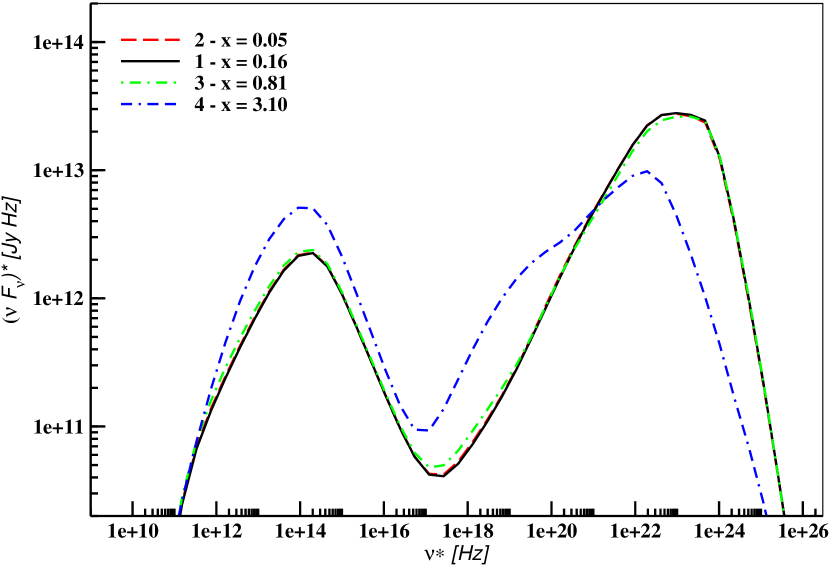
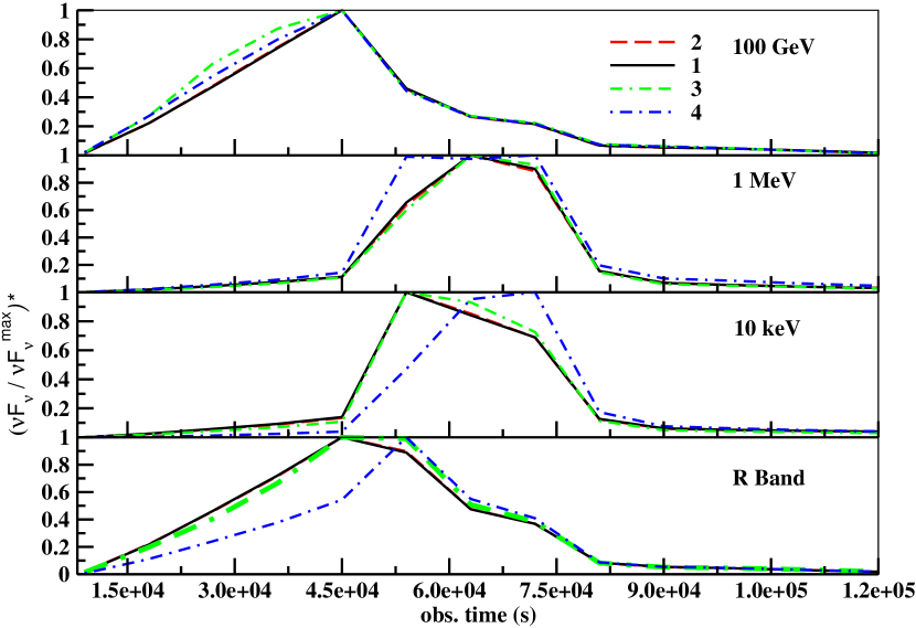
Figure 11: Simulated time-averaged SEDs (left) and light curves (right) of a generic blazar from runs 2, 3, and 4, illustrating the effects of varying the position, $z_{c}$, of the emission region along the jet axis. The plots are compared against those of run 1 (baseline model).

The right side of Fig. 11 shows a comparison of light curves for runs 2, 3, and 4 against those of run 1. As expected, the light curves of runs 2 and 3 essentially follow the same profile as those of run 1 due to the continued dominance of the ECBLR process in both these cases. As a result, the time taken for a pulse to peak and decline, in a particular energy band, is nearly the same for all three runs. However in the case of run 3, since the Compton cooling rate due to the ECBLR process is slightly less compared to that of run 1, for reasons mentioned above, there is a slight build-up of synchrotron photons for as long as the shocks are located within the emission region. This leads to a slightly extended feature in the synchrotron-dominated R-band pulse compared to that of run 1. On the other hand, in the case of run 4, due to a much reduced external Compton cooling rate compared to that of run 1 the entire broadband spectrum shifts to lower energies. Also, as explained above, this increases the dominance of synchrotron and SSC emission and allows them to persist for a longer duration compared to that of run 1. As a result, both the synchrotron-dominated R-band and SSC-dominated 10 keV pulses peak later than their run 1 counterparts. However, as explained in section 3.1, since the electrons responsible for the optical synchrotron pulse have higher energy compared to those responsible for the 10 keV pulse, they last only for as long as the shocks remain in the system. As a result, even though the R-band pulse for run 4 attains its peak later, it declines rapidly enough, once the FS exits the system, to match the decline of its run 1 counterpart, thereby making the duration of the R-band pulse for run 4 comparatively shorter. The 1 MeV pulse, on the other hand, is dominated by the peak of SSC emission and some contribution from the ECDT component. This implies that higher energy electrons than those emitting the synchrotron-dominated optical pulse are responsible for emission at this waveband. As a result, the pulse attains its peak sooner, exhibits a continued gradual buildup of photons, and lasts longer than its run 1 counterpart. As far as the 100 GeV pulse is concerned, the pulse profile is similar to that of run 1 due to reasons explained in section 3.1.

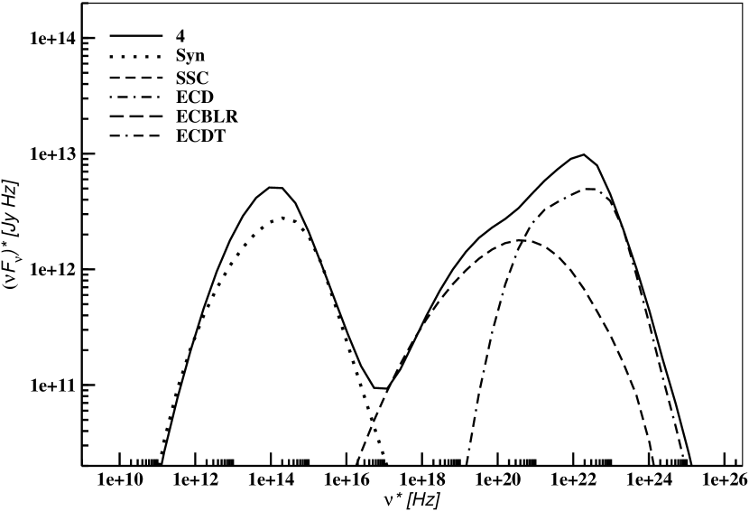
Figure 12: Time-averaged SED of run 4 showing the contribution of the individual radiation components as dotted: synchrotron; small-dashed: SSC; dot-dashed: ECD, which cannot be seen as its contribution is below $10^{10}$ Jy Hz; long-dashed: ECBLR, which also cannot be seen due to the reason stated above; and dot-double dash: ECDT.

3.2.2 Variations of BLR Covering Factor

Figure 13 shows the effect of varying the luminosity of the BLR (runs 5 & 6) on the time-averaged SED and light curves of the generic blazar with respect to our baseline model. This is equivalent to varying the BLR energy density, which directly affects the lower-energy component of a blazar. Changing $u_{\rm ph,BLR}$ shifts the partition between the synchrotron and the EC component, which in turn impacts the synchrotron flux of the SED. In the case of run 5, $L_{\rm BLR}$ is decreased such that $u^{\prime}_{\rm ph,BLR}$ evolves from $2.82\times 10^{-3}$ to $1.18\times 10^{-6}~{}erg~{}cm^{-3}$ over a distance of 1.04 pc. For run 6, $L_{\rm BLR}$ is increased such that $u^{\prime}_{\rm ph,BLR}$ evolves from $2.54\times 10^{-1}$ to $1.06\times 10^{-4}~{}erg~{}cm^{-3}$ over 1.04 pc. The starting position of the emission region for both runs is the same as that of run 1, with the FS exiting the system in the cavity of the BLR at $z\sim 0.16$ pc and the RS leaving the system when the emission region is located within the BLR at $z\sim 0.24$ pc.

As can be seen from the left side of Fig. 13, increasing the value of $L_{\rm BLR}$ (run 6), is equivalent to increasing the BLR radiation energy density. This leads to a dominance of the ECBLR component over the rest of the IC components, which increases the flux level of the EC component of the spectra and escalates the CDF by six times in comparison to its run 1 counterpart. This in turn, suppresses the SSC component well below the ECDT emission level. The locations of the transition and peak-EC-component frequencies also shift to higher values. This is because, in this case, the transition is no longer between synchrotron-SSC but between synchrotron-ECDT processes. As a result, the SH in the X-ray regime decreases to $\alpha^{*}_{\rm 2-10keV}=0.70$ because, as can be seen from the figure, the high-frequency end of the synchrotron component extends into the 2-10 keV regime, rendering the corresponding spectrum softer. On the other hand, since the emission at 10 GeV now comes from a harder part of the spectra, which is closer to the peak of the EC component compared to that of run 1, the Fermi range spectrum becomes harder and the SH increases to $\alpha^{*}_{\rm 10GeV}=2.50$. Contrary to the above scenario, decreasing the covering factor of the BLR to 0.01 (run 5), and thereby its $L_{\rm BLR}$, reduces the dominance of the ECBLR component and increases that of the ECDT component in producing high-energy emission compared to that of run 1. This can also be seen in Fig. 14, which shows the individual time-averaged radiation components responsible for the broadband time-averaged SED of run 5. In addition, due to the reduced BLR radiation energy density, the flux level of the EC component decreases compared to that of run 1. This in turn, lowers the CDF to 6.35 and shifts the locations of the transition and peak-EC-component frequencies leftward. Since the high-frequency end of the synchrotron compoent no longer extends into the X-ray range in this case, the SH of the SED in this regime increases to $\alpha^{*}_{\rm 2-10keV}=0.49$. On the other hand, the Fermi range SH, with $\alpha^{*}_{\rm 10GeV}=2.61$, is higher than that of run 1 but lower in comparison to run 6. This is because, in this case, the 10 GeV emission comes from the softer part of the HE component, which is well below the peak of the EC component, compared to that of run 6. In addition to this, there is weaker radiative cooling of particles due to EC processes compared to that of run 1. As a result, the corresponding Fermi range spectrum is harder than that of run 1, but softer than that of run 6.

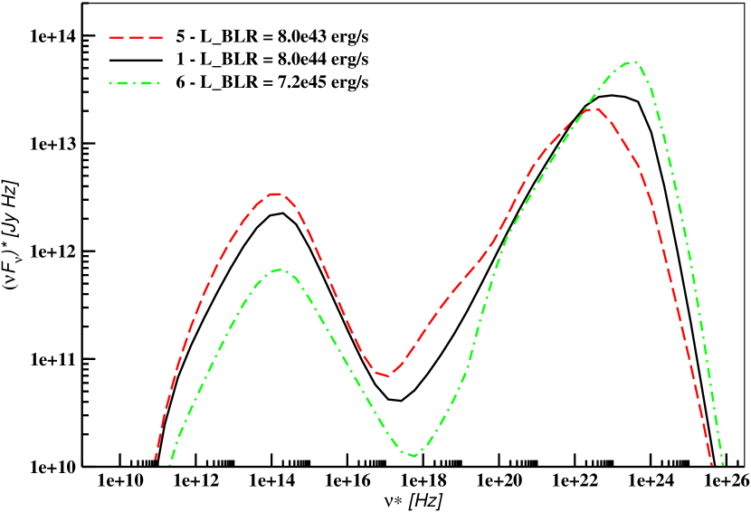
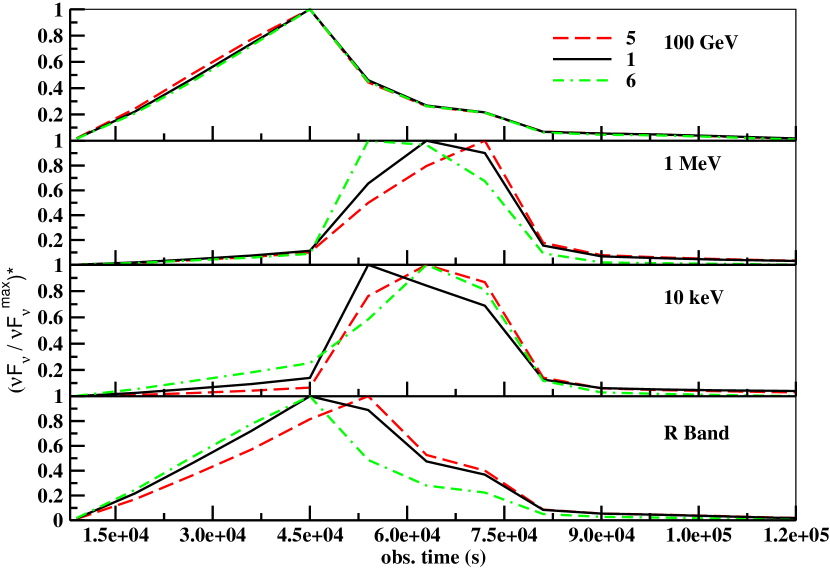
Figure 13: Simulated time-averaged SEDs (left) and light curves (right) of a generic blazar from runs 5 & 6, depicting the effects of varying the $L_{\rm BLR}$. The plots are compared against those of run 1 (baseline model).

The right side of Fig. 13 shows a comparison of light curves for runs 5 and 6 against those of run 1. The synchrotron R-band and 10 keV light curves for run 5 peak later compared to those of run 1. This is because, as explained above, a lower $u^{\prime}_{\rm ph,BLR}$ results in a reduced Compton cooling rate, which in turn affects the synchrotron flux and makes the synchrotron-dominated pulse last longer. As a result, the R-band light curve continues to rise for as long as the FS is in the system. But, as explained in section 3.2.1 for the case of run 4, since higher energy electrons are responsible for the optical synchrotron pulse than those for the 10 keV pulse, the optical pulse declines quickly enough to match the declining pulse profile of that of run 1, once the FS shock crosses the system at $t^{*}_{\rm FS,~{}exit}\sim$ 53 ks. The 1 MeV pulse, in the case of run 5, is dominated by the rising but softer part of the ECDT component. This implies that lower energy particles are responsible for producing this pulse, compared to those of run 1, thereby causing it to peak later. On the other hand, in the case of run 6, the R-band pulse exhibits exactly the opposite effect to that of run 5 due to an increased Compton cooling rate owing to a higher value of $u^{\prime}_{\rm ph,BLR}$. As a result, it declines much more rapidly and lasts for a shorter duration. The 10 keV pulse, in this case, is dominated by the low-frequency end of the ECDT process. As a result, the corresponding spectrum is softer because low-energy electrons are responsible for producing this pulse. This is why the pulse peaks later than that of run 1, but at the same time as that of run 5. The 1 MeV pulse, on the other hand, is dominated by the rising part of the ECBLR component and is due to higher energy electrons in the region, which is why the pulse starts to peak sooner, undergoes a gradual buildup, and declines faster compared to that of run 1. As far as the 100 GeV pulse for runs 5 and 6 is concerned, it follows the same profile as that of run 1 because of reasons explained in section 3.1.

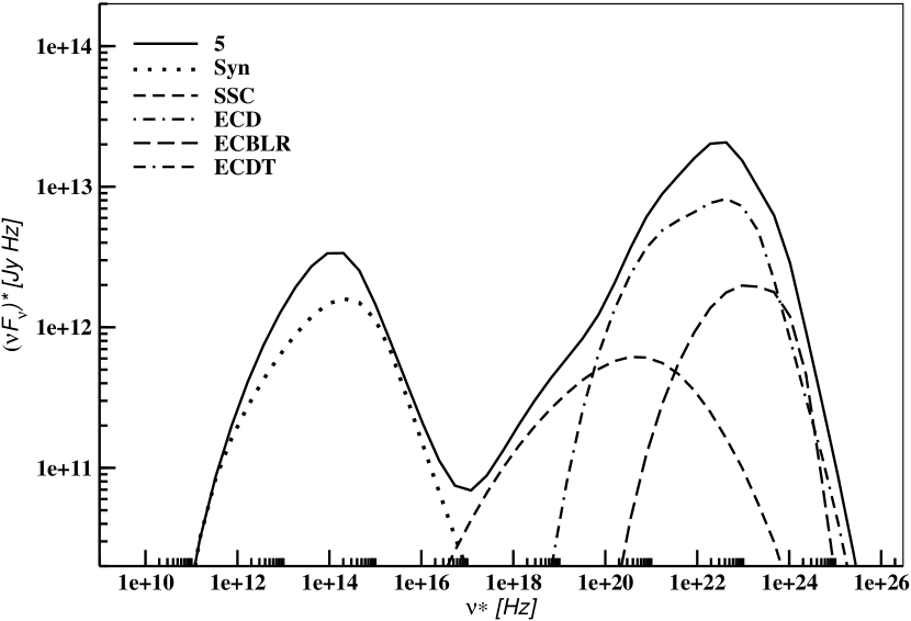
Figure 14: Time-averaged SED of run 5 showing the contribution of the individual radiation components as dotted: synchrotron; small-dashed: SSC; dot-dashed: ECD, which cannot be seen as its contribution is below $10^{10}$ Jy Hz; long-dashed: ECBLR, and dot-double dash: ECDT.

3.2.3 Variations of DT Covering Factor

The impact of decreasing (run 7) or increasing (run 8) the covering factor of the DT on the time-averaged SED and light curves of a generic blazar is shown in Fig. 15. This is equivalent to varying the DT energy density, which again affects the lower-energy component of a blazar and the location of the subsequent partition between the synchrotron and EC components. In the case of run 7, $f_{\rm cov,DT}$ is decreased such that $u^{\prime}_{\rm ph,DT}$ evolves from $5.25\times 10^{-3}$ to $4.14\times 10^{-3}~{}erg~{}cm^{-3}$ over a distance of 1.04 pc. For run 8, $f_{\rm cov,DT}$ is increased such that $u^{\prime}_{\rm ph,DT}$ evolves from $5.72\times 10^{-2}$ to $3.76\times 10^{-3}~{}erg~{}cm^{-3}$ over 1.04 pc. The starting position of the emission region for both runs is the same as that of run 1 with the FS exiting the system in the cavity of the BLR at $z\sim 0.16$ pc and the RS leaving the system when the emission region is located within the BLR at $z\sim 0.24$ pc.

Changing $f_{\rm cov,DT}$ also requires changing $R_{\rm out,DT}$, according to Eqs. (26) and (27), in order to keep the rest of the input parameters related to the ECDT emission the same. Decreasing $f_{\rm cov,DT}$ to 0.01 and increasing the size of the torus such that $R_{\rm out,DT}=2.37\times 10^{19}$ cm (run 7) dilutes the intensity of the ECDT emission. As a result, the contribution of the ECDT component to the EC emission decreases, which makes ECBLR the dominant EC component but lowers the overall EC flux level. Hence, the synchrotron emission rises, slightly decreasing the CDF to 10.1. The radiative cooling of particles due to EC emission decreases. This increases the SSC contribution in the X-ray regime, which consequently increases the SH such that $\alpha^{*}_{\rm 2-10keV}=0.57$. On the other hand, the effects of cooling due to the ECBLR component increase in the Fermi range, which decrease the SH at 10 GeV such that $\alpha^{*}_{\rm 10GeV}=2.77$. The peak EC-component frequency shifts to higher frequencies due to the dominance of the ECBLR component in this case. Contrary to the above scenario, increasing $f_{\rm cov,DT}$ to 0.9 and shrinking the DT such that $R_{\rm out,DT}=3.95\times 10^{18}$ cm (run 8) enhances the emission of the torus as received by the emission region. This makes the contribution of the ECDT component comparable to that of the ECBLR emission, as can be seen from Fig. 16. This has the opposite effect to that of run 7, although the overall change in the SED, in this case, is not as significant and closely follows that of run 1. To summarize the impact, the CDF increases slightly to 14.6 and the peak EC-component frequency shifts slightly to lower frequencies. The SH in the X-ray regime decreases slightly compared to that of run 1, while the SH at 10 GeV increases slightly such that $\alpha^{*}_{\rm 10GeV}=2.73$. This is because, in this case, the contribution of the ECBLR component decreases slightly compared to that of run 1, which implies comparatively less cooling and the presence of more higher-energy electrons, which gives rise to a harder spectra at that energy range.

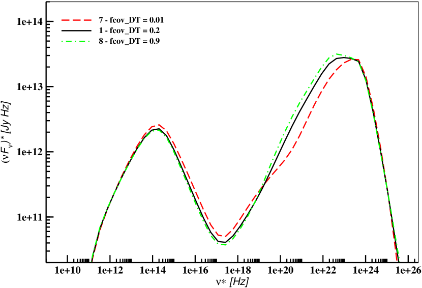
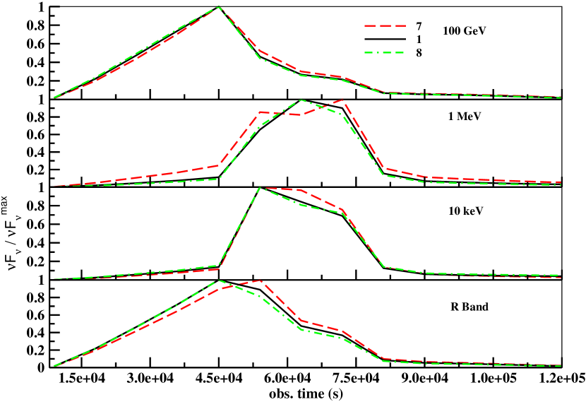
Figure 15: Simulated time-averaged SEDs (left) and light curves (right) of a generic blazar from runs 7 & 8 showing the effects of changing the covering factor of the DT and consequently $R_{\rm out,DT}$ according to Eqs. (26) and (27).

The right side of Fig. 15 compares light curves for runs 7, and 8 against those of run 1. As can be seen from the figure, the light curve profiles of run 8 are similar to those of run 1 because the overall impact of increasing the covering factor of the DT, while keeping other parameters related to EC emission the same, is not very significant. On the other hand, in the case of run 7, the synchrotron-dominated R-band pulse lasts for a slightly longer duration due to a decreased Compton cooling rate and consequently an increased amount of synchrotron emission. As a result, it peaks later than that of run 1 but lasts only for as long as the FS is inside the emission region and declines afterwards due to the reasons given in section 3.1. At 10 keV, the pulse of run 7 peaks at the same time and has a similar profile as that of run 1, but lasts a bit longer due to an increased contribution from the SSC emission. On the other hand, unlike the case for run 1, the 1 MeV emission in run 7 is dominated by the rising part of the ECBLR component involving comparatively lower-energy electrons. As a result, the corresponding pulse peaks later before declining along with those of runs 1 and 8. We would like to point out here that the 1 MeV light curve for run 7 has really only one peak. The slight depression seen at around 63000s is more of a numerical artifact resulting due to the not-so-high resolution of the electron and photon energy grid. As is seen in the other cases, the 100 GeV pulse for runs 7 and 8 follows the same profile as that of run 1 because of reasons explained in section 3.1.

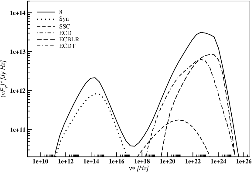
Figure 16: Time-averaged SED of run 8 showing the contribution of the individual radiation components as dotted: synchrotron; small-dashed: SSC; dot-dashed: ECD, which cannot be seen as its contribution is below $10^{10}$ Jy Hz; long-dashed: ECBLR, and dot-double dash: ECDT.

4 Discussion and Conclusions

We have extended the scope of the multi-zone time-dependent leptonic jet model, with radiation feedback scheme, in the internal shock scenario, of Joshi & Böttcher (2011) (known for short as the MUlti ZOne Radiation Feedback, MUZORF, model) to include the EC component by considering anisotropic target radiation fields. The current model is now applicable to a broader class of blazars, including FSRQs, LBLs, and IBLs, and allows us to distinguish and quantify the contribution of each of the seed photon fields in producing high-energy emission of blazars out to $\sim$ pc scales.

In our approach, we consider three sources of seed photon fields, namely the accretion disk, the BLR, and the DT. We let the system evolve to beyond the BLR and into the DT, and calculate the corresponding distance- and time-dependent EC emission according to the prescription described in sections 2.1 to 2.3. In our current work, we have not considered detailed spectral fitting and analysis to compare against the multiwavelength SEDs and light curves of blazars available through campaigns involving the Fermi Gamma Ray Space Telescope, which we leave to future work. Instead, we have carried out a parameter study of rapid variability, on timescales of $\sim$ 1 day, between optical, X-ray, and $\gamma$-ray energies. We point out that the MUZORF model is applicable to EC emission up to only a few parsecs. This is because currently it does not include adiabatic cooling, which is relevant for evolving the system out to several parsecs. This is a work in progress that we plan to address in the future.

We have carried out a parameter study to understand the effects of varying input parameters relevant to the EC emission on the dynamic evolution of the SED and light curves of a generic blazar. A number of input parameters, such as the location of the emission region along the jet axis ($z_{c}$), the covering factor of the BLR ($f_{\rm cov,BLR}$), and that of the dusty torus ($f_{\rm cov,DT}$) were varied. The goal of the study was to understand the dependence of the contribution of each of the target photon field components on such parameters in producing HE emission of blazars. Anisotropic target radiation fields were considered from each of the seed photon field components in order to enable the system to evolve beyond the BLR and allow the contribution of each of the three components to be incorporated as accurately as possible. As has been demonstrated in §2.3, the range of angles covered by incoming DT photons, in the anisotropic case, is quite narrow. For the cases considered here, the DT played an important role in contributing toward $\gamma$-ray emission in the MeV range, while the BLR contributed mostly in the high MeV - low GeV range. For the value of $L_{\rm disk}$ and $z_{c}$ considered in all of our cases, the emission due to the ECD process was found to be negligible for the level of fluxes considered here. This is because of the amount of de-boosting of disk photons when entering the jet from behind or from the side at those positions. Similar evolution of the ECD emission with $z_{c}$ was also found by Dermer et al. (2009).

For all cases, the 100 GeV light curves always led the X-rays and MeV emission, while for some cases they either led or peaked at the same time as the optical light curves, depending on the parameter that was varied for those simulations. More symmetric pulse profiles were obtained for higher frequency light curves than those for lower frequency ones. Similar behavior of pulse profiles were also found by Sokolov & Marscher (2005); Böttcher & Dermer (2010); Joshi & Böttcher (2011). It was demonstrated, that for the case where the emission region was placed beyond the BLR, the HE emission was primarily due to ECDT and SSC processes. This can be extrapolated to conclude that as the distance of the emitting plasma from the central engine increases, SSC starts to dominate over EC emission due to a substantially reduced amount of Doppler boosting of incoming seed photon fields. The EC losses then become a fraction of the synchrotron losses, and SSC flux exceeds the EC flux (Sokolov & Marscher, 2005). Similar results are achieved if the energy density of the BLR or DT radiation is reduced, which also introduces an optical lag relative to the HE $\gamma$-ray variations (Böttcher & Dermer, 2010). In addition to these input parameters, another factor that plays an important role in deciding the duration of HE pulses and the range of the location of $\gamma$-ray emission is the time of exit of shocks from their respective emitting regions. This is because, as discussed in §3, $\gamma$-ray emission is produced by highly energetic leptons, which, in turn, are produced in the system for as long as the shocks are present and accelerating particles to such high energies. Therefore, analyzing the effects of the combination of the factors discussed above on the evolution of the system is crucial to understanding the origin of $\gamma$-ray emission and its relationship with emission at lower frequencies.

Understanding of the sources of seed photons is imperative in order to comprehend the HE emission of blazars in general. At the same time, it is important to realize that at distances of several parsecs from the central engine, the target photon field from these components is quite weak. In that case, these three conventional sources might not explain the high $\gamma$-ray luminosity and correlation between $\gamma$-ray and radio events that have been observed at such distances (Jorstad et al., 2013; Marscher et al., 2012; Agudo et al., 2011). In such a scenario, considering possible new sources of seed photon fields or modifying the placement of the existing ones becomes important. The latter might include, (1) a variable location of the $\gamma$-ray emitting zone (Stern & Poutanen, 2011), (2) an outflowing BLR serving as a source of external seed photons at parsec scales (León-Tavares et al., 2011), (3) the presence of some stray BLR material surrounding the radio core that could produce required density of target photons at those distances (León-Tavares et al., 2013), or (4) an additional but internal source of seed photons, such as a Mach disk, in tandem with DT photon field (Marscher, 2013). Such possibilities should be explored in producing the $\gamma$-ray luminosity at those length scales.

Appendix A Lines of Sight of Incoming BLR Photons

Here we calculate the respective path lengths of incoming BLR photons for Pos. 1, 2, and 3 of the emission region, as described in §2.2. These path lengths are used to integrate the emission coefficient to obtain the intensity of incoming photons (in units of $erg~{}s^{-1}cm^{-2}ster^{-1}$) as a function of distance, z, along the jet axis and angle $\theta$. All quantities in this section refer to the lab frame. Referring to Fig. 4, the quantity $s$ is considered as $l$ in this section. Then, the values of $l_{\rm min}$ and $l_{\rm max}$ of an incoming BLR photon when the emission region is located at Pos. 1 are obtained using the cosine law of angles:

$$r^{2}=z^{2}+l^{2}-2zl\cos{\theta}~{}.$$ (A1)

Given $R_{\rm in}$ and $R_{\rm out}$, we obtain the respective pathlength limits, $l_{\rm min}$ and $l_{\rm max}$, as

$$l_{\rm min}=z\cos{\theta}+z\sqrt{\cos^{2}{\theta}+\left(\frac{R_{\rm in}}{z}\right)^{2}-1}~{},$$

$$l_{\rm max}=z\cos{\theta}+z\sqrt{\cos^{2}{\theta}+\left(\frac{R_{\rm out}}{z}\right)^{2}-1}~{},$$ and

$$I(z,\theta)=\int\limits_{l_{\rm min}}^{l_{\rm max}}j(r)dl~{},$$ (A2)

where $j(r)$ is the emission coefficient at the radial distance $r$, as described in §2.2 and Liu & Bai (2006). Similarly, when the emission region is located at Pos. 2, the limits of integration can be calculated using the method described above, while keeping in mind that, for this case, $z>R_{\rm in}$. As a result, we obtain

$$l_{\rm min,min}=z\cos{\theta}-z\sqrt{\cos^{2}{\theta}+\left(\frac{R_{\rm in}}{z}\right)^{2}-1},$$

$$l_{\rm min,max}=z\cos{\theta}+z\sqrt{\cos^{2}{\theta}+\left(\frac{R_{\rm in}}{z}\right)^{2}-1},$$ and

$$l_{\rm max}=z\cos{\theta}+z\sqrt{\cos^{2}{\theta}+\left(\frac{R_{\rm out}}{z}\right)^{2}-1},$$ such that

$$I(z,\theta)=\int\limits_{0}^{l_{\rm min,min}}j(r)dl+\int\limits_{l_{\rm min,max}}^{l_{\rm max}}j(r)dl~{}.$$ (A3)

For $\theta\geq\theta_{\rm cr}$, where $\theta_{\rm cr}=\cos^{-1}(\frac{l_{\rm cr}}{z})$ and $l_{\rm cr}=\sqrt{z^{2}-R^{2}_{\rm in}}$, there is no contribution from lines of sight through the cavity of the BLR. In this case, the intensity calculation reduces to $I(z,\theta)=\int\limits_{0}^{l_{\rm max}}j(r)dl$, where $l_{\rm max}$ is given in Eq. (A).

For the case where the emission region is located at Pos. 3, critical angles and their corresponding path lengths to the outer boundary of the inner and outer circles, respectively, are given by

$$\theta_{\rm in,cr}=\cos^{-1}{(\frac{l_{\rm in,cr}}{z})},$$

$$l_{\rm in,cr}=\sqrt{z^{2}-R^{2}_{\rm in}},$$ and

$$\theta_{\rm out,cr}=\cos^{-1}{(\frac{l_{\rm out,cr}}{z})},$$

$$l_{\rm out,cr}=\sqrt{z^{2}-R^{2}_{\rm out}}~{}.$$ (A4)

Thus, if $\theta<\theta_{\rm in,cr}$, the intensity would be obtained according to

$$l_{\rm min,min}=z\cos{\theta}-z\sqrt{\cos^{2}{\theta}+\left(\frac{R_{\rm in}}{z}\right)^{2}-1},$$

$$l_{\rm min,max}=z\cos{\theta}+z\sqrt{\cos^{2}{\theta}+\left(\frac{R_{\rm in}}{z}\right)^{2}-1},$$ and

$$l_{\rm max,min}=z\cos{\theta}-z\sqrt{\cos^{2}{\theta}+\left(\frac{R_{\rm out}}{z}\right)^{2}-1},$$

$$l_{\rm max,max}=z\cos{\theta}+z\sqrt{\cos^{2}{\theta}+\left(\frac{R_{\rm out}}{z}\right)^{2}-1},$$ such that

$$I(z,\theta)=\int\limits_{l_{\rm max,min}}^{l_{\rm min,min}}j(r)dl+\int\limits_{l_{\rm min,max}}^{l_{\rm max,max}}j(r)dl~{}.$$ (A5)

If $\theta_{\rm in,cr}\leq\theta<\theta_{\rm out,cr}$, the intensity is given by

$$l_{\rm max,min}=z\cos{\theta}-z\sqrt{\cos^{2}{\theta}+\left(\frac{R_{\rm out}}{z}\right)^{2}-1},$$

$$l_{\rm max,max}=z\cos{\theta}+z\sqrt{\cos^{2}{\theta}+\left(\frac{R_{\rm out}}{z}\right)^{2}-1},$$ such that

$$I(z,\theta)=\int\limits_{l_{\rm max,min}}^{l_{\rm max,max}}j(r)dl~{},$$ (A6)

References

- Abdo et al. (2010) Abdo, A. A., et al., 2010, ApJ, 716, 30
- Agudo et al. (2011) Agudo, I., et al., 2011, ApJL, 735, 10
- Albert et al. (2008) Albert, J., et al., 2008, Science, 320, 1752
- Aleksić et al. (2012) Aleksić, J., et al., 2012, A & A, 542, 100
- Blandford & Levinson (1995) Blandford, R. D., & Levinson, A., 1995, ApJ, 441, 79
- Błażejowski et al. (2000) Błażejowski, M., Sikora, M., Moderski, R., & Madejski, G. M., 2000, ApJ, 545, 107
- Bloom & Marscher (1996) Bloom, S. D., & Marscher, A. P., 1996, ApJ, 461, 657
- Böttcher (2012) Böttcher, M., 2012, Fermi & Jansky Proceedings, arXiv:1205.0539
- Böttcher & Bloom (2000) Böttcher, M., & Bloom, S. D., 2000, AJ, 119, 469
- Böttcher & Dermer (2010) Böttcher, M., & Dermer, C. D., 2010, ApJ, 711, 445
- Böttcher, Mause, & Schlickeiser (1997) Böttcher, M., Mause, H., & Schlickeiser, R., 1997, A&A, 324, 395
- Böttcher & Reimer (2004) Böttcher, M., & Reimer, A., 2004, ApJ, 609, 576
- Böttcher, Reimer, & Marscher (2009) Böttcher, M., Reimer, A., & Marscher, A. P., 2009, ApJ, 703, 1168
- Chiaberge & Ghisellini (1999) Chiaberge, M., & Ghisellini, G., 1999, MNRAS, 306, 551
- Collmar et al. (2010) Collmar, W., et al., 2010, A & A, 522, 66
- Dermer et al. (2009) Dermer, C. D., Finke, J. D., Krug, H., & Böttcher, M., 2009, ApJ, 696, 32
-
Dermer & Menon (2009)
Dermer, C. D., & Menon, G., 2009, High Energy Radiation from Black
Holes:
Gamma Rays, Cosmic Rays, and Neutrinos, Princeton University Press - Dermer & Schlickeiser (2002) Dermer, C. D., & Schlickeiser, R., 2002, ApJ, 575, 667
- Dermer & Schlickeiser (1994) Dermer, C. D., & Schlickeiser, R., 1994, ApJS, 90, 945
- Dermer & Schlickeiser (1993) Dermer, C. D., & Schlickeiser, R., 1993, ApJ, 416, 458
- Dermer, Sturner, & Schlickeiser (1997) Dermer, C. D., Sturner, S. J., & Schlickeiser, R., 1997, ApJS, 109, 103
- Donea & Protheroe (2003) Donea, A-C., & Protheroe, R. J., 2003, Astroparticle Physics, 18, 377
- Finke, Dermer, & Böttcher (2008) Finke, J. D., Dermer, C. D., & Böttcher, M, 2008, ApJ, 686, 181
- Francis et al. (1991) Francis, P., et al., 1991, ApJ, 373, 465
- Gaskell, Shields, & Wampler (1981) Gaskell, C. M., Shields, G. A., & Wampler, E. J., 1981, ApJ, 249, 443
- Ghisellini & Madau (1996) Ghisellini, G., & Madau, P., 1996, MNRAS, 280, 67
- Ghisellini & Tavecchio (2009) Ghisellini, G., & Tavecchio, F., 2009, MNRAS, 397, 985
- Jorstad et al. (2013) Jorstad, S. G., et al., 2013, ApJ, 773, 147
- Jorstad et al. (2005) Jorstad, S. G., et al., 2005, AJ, 130, 1418
- Joshi & Böttcher (2011) Joshi, M., & Böttcher, M., 2011, ApJ, 727, 21
- Kaspi & Netzer (1999) Kaspi, S., & Netzer, H., 1999, ApJ, 524, 71
- Kataoka et al. (1999) Kataoka, J., et al., 1999, ApJ, 514, 138
- Kusunose & Takahara (2005) Kusunose, M., & Takahara, F., 2005, ApJ, 621, 285
- León-Tavares et al. (2013) León-Tavares, J., et al., 2013, ApJL, 763, 36
- León-Tavares et al. (2012) León-Tavares, J., et al., 2012, ApJ, 754, 23
- León-Tavares et al. (2011) León-Tavares, J., et al., 2011, A&A, 532, 146
- Lindfors, Valtaoja, & Türler (2005) Lindfors, E. J., Valtaoja, E., & Türler, M., 2005, A&A, 440, 845
- Liu & Bai (2006) Liu, H. T., & Bai, J. M., 2006, ApJ, 653, 1089
- Malmrose et al. (2011) Malmrose, M., et al., 2011, ApJ, 732, 116
- Marscher et al. (2012) Marscher, A. P., et al., 2012, Fermi & Jansky Proceedings, arXiv:1204.6706
- Marscher (2013) Marscher, A. P., 2013, submitted to ApJ
-
Rybicki & Lightman (1979)
Rybicki, G. B., & Lightman, A. P., 1979, Radiative processes in
astrophysics,
John Wiley & Sons, New York - Shakura & Sunyaev (1973) Shakura, N. I., & Sunyaev, R. A., 1973, A & A, 24, 337
- Sikora et al. (1994) Sikora, M., Begelman, M. C., & Rees, M. J., 1994, ApJ, 421, 153
- Sikora et al. (1997) Sikora, M., Madejski, G., Moderski, R., & Poutanen, J., 1997, ApJ, 484, 108
- Sokolov & Marscher (2005) Sokolov, A., & Marscher, A. P., 2005, ApJ, 629, 52
- Stern & Poutanen (2011) Stern, B. E., & Poutanen, J., 2011, MNRAS, 417, L11