Initial Speed of Knots in the Plasma Tail of C/2013 R1(Lovejoy)

Abstract

We report short-time variations in the plasma tail of C/2013 R1(Lovejoy). A series of short (two to three minutes) exposure images with the 8.2-m Subaru telescope shows faint details of filaments and their motions over 24 minutes observing duration. We identified rapid movements of two knots in the plasma tail near the nucleus ($\sim$ 3$\times 10^{5}$ km). Their speeds are 20 and 25 km s^-1 along the tail and 3.8 and 2.2 km s^-1 across it, respectively. These measurements set a constraint on an acceleration model of plasma tail and knots as they set the initial speed just after their formation. We also found a rapid narrowing of the tail. After correcting the motion along the tail, the narrowing speed is estimated to be $\sim$ 8 km s^-1. These rapid motions suggest the need for high time-resolution studies of comet plasma tails with a large telescope.

1 Introduction

Plasma tails of comets and their time variations potentially provide crucial information on solar winds and magnetic fields in the solar system (e.g., Niedner, 1982; Mendis, 2006; Downs et al., 2013). Short-time variations in plasma tails, however, are not yet fully understood. Indeed, most previous studies observed tails and structures at far distances ($>10^{6}$ km from the nucleus) with a time resolution of an order of an hour.

Regarding the speed of movement along the tail, Niedner (1981) studied 72 disconnection events (DEs) of various comet tails and found $\lesssim$ 100 km s^-1 at $\lesssim 10^{7}$ km from the nuclei. Their initial speeds before DEs are around 44 km s^-1 and the typical acceleration is 21 cm s^-2. Saito et al. (1987) analyzed a knot in the plasma tail of comet 1P/Halley and derived its average velocity of 58 km s^-1 at 4–9 $\times 10^{5}$ km from the nucleus. Kinoshita et al. (1996) observed C/1996 B2(Hyakutake) and measured the speed of a knot of 99.2 km s^-1 at 5.0 $\times 10^{6}$ km from the nucleus. Brandt et al. (2002) investigated DE of C/1995 O1 (Hale-Bopp) and obtained the speed of $\sim$ 500 km s^-1 at $\sim$ 7$\times 10^{7}$ km from the nucleus. Buffington et al. (2008) analyzed several knots in comets C/2001 Q4(NEAT) and C/2002 T7(LINEAR) using the Solar Mass Ejection Imager. They found the speed to be 50–100 km s^-1 around $10^{6}$ km from the nucleus.

These previous studies did not catch the moment immediately after the formation of knots or the detachment of knots from the tail. The initial speed at these critical times was only an extrapolation from later observations relatively far away. In this letter, we report detections of knots in the plasma tail 3$\times 10^{5}$ km away from the nucleus of C/2013 R1(Lovejoy) and a direct measurement of their initial motions. We adopt the AB magnitude system throughout the paper.

2 Data

The comet was observed on 2013 December 4 (UT) using the Subaru Prime Focus Camera (Suprime-Cam; Miyazaki et al., 2002) mounted on the Subaru Telescope at Mauna Kea (observatory code 568). The camera consists of a 5 $\times$ 2 array of 2k $\times$ 4k CCDs. The pixel scale is 0.202 arcsec pixel^-1. The field of view is about 35$\times$28 arcmin. We used two broadband filters: W-C-IC (I-band: center=7970 Å, full width at half maximum (FWHM)=1400Å) and W-J-V (V-band: center=5470 Å, FWHM=970Å) filters. Both bands trace the plasma tail. I-band includes predominantly H₂O⁺ line emissions, while V-band includes CO⁺ and H₂O⁺ line emissions.

The observation log is given in Table 1. The total observing time of 24 minutes was spent after main science targets of the observing run were set. The start time of the exposures have an uncertainty of about 1 second. The position angle and the pointing offset were adopted to catch the comet nucleus at the bottom-left corner and to have the tail run diagonally across the field-of-view so that the maximum extent of the tail is framed in each exposure.

The Subaru telescope’s non-sidereal tracking mode(Iye et al., 2004) was used so that the comet was always observed at the same position on the CCD array. For the observing run, the comet’s coordinates were calculated using the NASA/JPL HORIZONS system with the orbit element of JPL#22. We used an ephemeris of one-minute step. Unfortunately, the values of JPL#22 were not recorded. In the following, we instead used newer orbital elements (JPL#55). The values are given in Table 2. The positions calculated from JPL#22 and JPL#55 have an offset by 0.34 arcsec in right ascension and -1.88 arcsec in declination but show no drift during the observation. The offset of the absolute celestial coordinate does not affect in this study, since our analysis is on relative position of structures inside of the comet. At the time of the observations, the observercentric and heliocentric distance to the comet were 0.5523–0.5526 and 0.8812–0.8811 au, respectively. In the sky projection, the conversion from the angular to the physical scales was 400.6–400.8 km arcsec^-1. Considering the phase angle (sun-target-observer angle) of 83.5 degrees at the time of the observations, we adopt the physical scale along the tail of 403.3 km arcsec^-1 in the following discussion. The heliocentric ecliptic coordinate of the comet nucleus was ($\lambda$,$\beta$)=(87.5,30.7). The comet was located before the perihelion passage, and its heliocentric velocity was -12.6 km s^-1.

The seeing size is estimated from short (two-second) exposures and was 1.0 and 1.1 arcsec in I and V-bands, respectively. The movement of the comet in the celestial coordinate was about (dRA$\times$cos(D)/dt,d(D)/dt)=(283 – 284,-115) arcsec hr^-1 during the observations. Due to the non-sidereal tracking, stars move in an exposure, but this motion does not affect the measurement of the seeing size significantly since the shift is only about 0.17 arcsec in a two-second exposure.

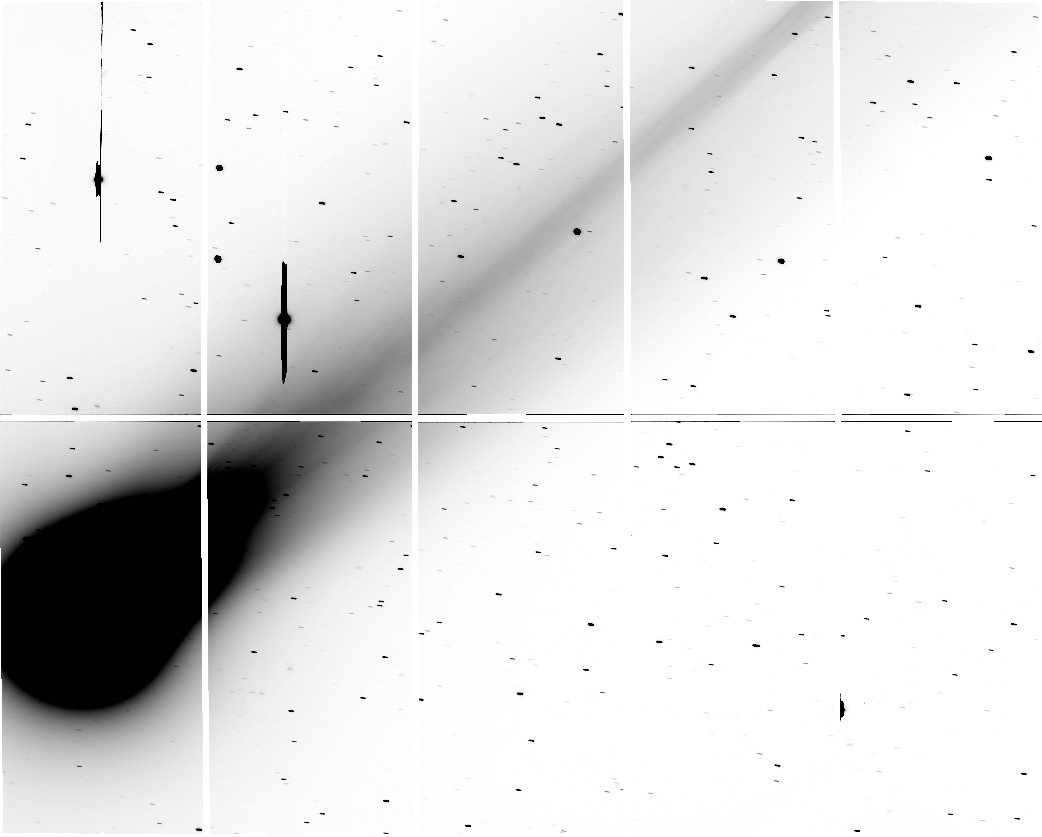
Figure 1: An example of the data (V1; see Table 1). The bright part is shown as black. Suprme-Cam consists of 10 CCDs, and the gaps between chips are shown in white. The field of view is 34$\times$27 arcmin.

The data was reduced in a standard manner; the steps include overscan subtraction, crosstalk correction (Yagi, 2012), flat fielding using twilight flat, and distortion correction. The relative flux and relative position among the CCDs are calibrated using other dithered datasets taken in the same night. The mosaicked image of V1 (Table 1) is shown as Figure 1 as an example.

The flux was calibrated against stars in the field using the Eighth Data Release of the Sloan Digital Sky Survey (SDSS DR8; Aihara et al., 2011) catalog in the same way as in Yagi et al. (2013). We first used SExtractor (Bertin & Alnouts, 1996) for object detection in the Suprime-Cam images and astrometric calibration was performed to the center of the elongated stars against the Guide Star Catalog 2.3.3 (Lasker et al., 2008). Then, we measured aperture fluxes at each position of SDSS star whose r-band magnitude is 16$<$r$<$20. The aperture radius was 40, 50, and 60 pixels, and we used

$$F=F(40)-\left[(F(60)-F(50))\times\frac{40^{2}}{60^{2}-50^{2}}\right]$$ (1)

as the background-corrected aperture flux of an elongated star, where $F(r)$ is the aperture flux of $r$ radius. Photometric zero point was estimated from the instrument flux $F$ and the catalog magnitude converted to the Suprime-Cam AB system. The color conversion coefficients from SDSS to Suprime-Cam magnitudes are given in Table 3. The K-correct (Blanton & Roweis, 2007) v4 offset for SDSS is applied; $m_{AB}-m_{SDSS}$=0.012, 0.010 and 0.028 for $g$, $r$ and $i$, respectively. The number of stars used for calibration was $\sim 290$ in V and $\sim 410$ in I. The measured photometric zero-point of chip 2 (reference chip) was 27.36(I) and 27.15(V) AB mag per 1 ADU s^-1, and the peak-to-peak variation among exposures were smaller than 0.02 mag in each band. These zero points are comparable to the ones derived typically under photometric conditions, and thus we regard the data as having been obtained under photometric conditions.

3 Result

3.1 Image Processing

To investigate the fine structures in the plasma tail, additional image processing was applied. First, we rotate the image counterclockwise by 50 degrees so that the plasma tail aligns to the y-axis, and the region around the plasma tail within full width of 1000 pixels (3.4 arcmin) was extracted. The position angle of the image to the north is the same among the nine images (160.0 degree). In the coordinate, the sun lay in the direction of (x,y)=(-0.014,+1.000). The nuclei position was measured in short exposures (I2 and V2). The relative positional consistency among the images depends on the accuracy of the non-sidereal tracking mode of the Subaru telescope. As we used the ephemeris of a one-minute step, enough accuracy is guaranteed.

We then applied an unsharp masking technique to each image; we convolved the extracted images with various sizes of Gaussian filter ($\sigma$=10, 20, 30, 50, 75 pixels) and subtracted the smoothed image from the original ones. The details are presented in Appendix A. This processing removes larger structures and enhances fine structures. To differentiate the processing with different kernel sizes, we refer to each as highpass${\it\sigma}$, e.g., highpass10 when processed with the Gaussian with $\sigma$=10 pixels. Bright stars in the background contaminate small features associated physically with the cometary tail (e.g., knots), and hence, we iteratively masked them. Finally, we binned the image by 5$\times$5 pixels (1.01 arcsec square). Figure 2 shows six longer-exposure images after the processing. These images show the gaps between CCD chips as gray bands. Brightening/darkening around chip edges are artifacts. These do not affect the following analyses.

3.2 Moving Knots

We can visually see two knots moved downstream around the distance of $\sim$ 3$\times 10^{5}$ km from the nucleus (indicated by arrows in Figure 2). The closeup images are shown as Figure 4. One of the knots first appears to be connected to the global filamentary structures running along the tail. It later becomes detached from the structures. The positions of the knots are measured by running SExtractor (Bertin & Alnouts, 1996) on the 5$\times$5 binned unsharp masked images. We measured in highpass30, highpass50, highpass70, and highpass90 images. As examined in Appendix B, an unsharp masking with a smaller kernel may introduce larger positional errors. Meanwhile, the knot may not be detected after an unsharp masking with a large kernel because it is buried in global features. We therefore adopted the position from the largest kernel in which the peak of the knot is detected. The root mean squares (rms) of the position was $\sim 6\times 10^{2}$ km.

Distances from the nucleus (along the tail; y-axis) and offsets from the tail axis (perpendicular to the tail; x-axis) are plotted as a function of time in Figure 4. 20 and 25 km s^-1 along the tail and 3.8 and 2.2 km s^-1 across the tail, respectively. The motion should make the shape of the knots elongated in a two-minute exposure by 6–7 arcsec along the tail and 1.3 or 0.7 arcsec across the tail. Since the size of the knots is at least 10–15 arcsec in diameter, elongation by the motion had little effect on the size estimation.

These knot motions show tilts from the central axis of the tail by about 0.1–0.2 radians (6–11 degrees). We note that the direction to the Sun is 0.014 radians (0.8 degrees) from the axis, and therefore, the knot motions are not in a perfect alignment to the direction to the Sun.

The distances to the knots from the nucleus change almost linearly with time in Figure 4. The effect of acceleration is therefore small in the short duration of our observations (23 minutes). The clear detection of the spatial motions, however, indicates the potential for direct measurements of the acceleration in future. If we can take the accelerations of previous measurements of other comets by Niedner (1981) (21 cm s^-2), the expected change in the speed is only 0.3 km s^-1 in 23 minutes. If we adopt 17 cm s^-2, which is calculated from Figure 4 of Saito et al. (1987) as 2.4 km s^-1 increment is seen in four hours, the expected change in the speed during our observation is even smaller (0.2 km s^-1). Therefore, a sequence of few hours observations of a knot would permit us to measure the acceleration.

3.3 Change of tail width in I-band

We found that the width of the plasma tail also rapidly changed. In the analysis, the original images before the unsharp masking were used. In Figure 5 and Figure 6 show spatial surface brightness profiles across the tail and their time variation. Since we have measured the motions of the knots (presumably the motion of the tail), we can track the variation in the tail width at a comoving position as the tail would flow at the speed of $\sim$ 22 km s^-1. In a sequence of images (I1, I3, and I4), we measured a profile at the distance of 6$\times$10⁵ km in I1. We then tracked the location of the material initially at this distance, but at later times using the flow speed, and plotted the profiles of (presumably) the same material in I3 and I4. The tail width is determined at the surface brightness of 21.3 AB magnitude arcsec^-2 in I-band. It narrowed from 2.4$\times 10^{4}$ to 2.0$\times 10^{4}$, and then to 1.8$\times 10^{4}$ km for I1, I3, and I4, respectively.

From this measurement, the speed of the narrowing motion across the tail is $\sim$ 8 km s^-1 at each edge. The center of the light distribution, meanwhile, did not show any notable change (Figure 6). This narrowing speed is larger than those of the knots in the same direction perpendicular to the tail (3.8 and 2.2 km s^-1; Section 3.2). This apparent difference could be attributed to a projection of the motion of the knots in the sky.

If we assume every fine structure (filamentary structure) in the tail is moving at $\sim$ 8 km s^-1 perpendicular to the tail, the amount of spatial shift would be about 2.5 arcsec within the 120-second exposures. On the other hand, the fine structures appear to be a typical 5 –10 arc sec width in short exposures (I2, V2). Therefore, the blur due to the motions during a single 120-second exposure should not affect the positional measurements of the structures much.

4 Discussion and Summary

The initial speeds of two moving knots ($\sim$ 22 km s^-1) are significantly slower than the ones measured by Niedner (1981) (44 km s^-1; rms of 10.9 km s^-1). This speed is also smaller than that measured in comet Halley by Saito et al. (1987) (58 km s^-1), who suggested that the velocity was constant at 4–9 $\times 10^{5}$ km from the nucleus.

Though it is not clear what the dominant factor of the initial speed of knots is, we can compare several parameters of the comets. As the data used by Niedner (1981) include information from various comets, we compare parameters with the single case of the comet Halley by Saito et al. (1987). At the observation by Saito et al. (1987), the heliocentric distance to comet Halley was 1.016 au, the heliocentric ecliptic coordinate was ($\lambda$,$\beta$)=(30.1,8.8), and the heliocentric velocity was -26.5 km s^-1. Compared with C/2013 R1(Lovejoy) in this study, a part of the difference in the initial speed may be explained by the difference in the heliocentric velocity of the nucleus, -12.6 km s^-1 versus -26.5 km s^-1, if we assume that the initial speed of the knots might be comparable in heliocentric frame. It, however, does not fully explain $\sim$ 40 km s^-1 difference. Another difference is heliocentric ecliptic latitude, 30.7 vs 8.8, which may result in the difference in the speed of the solar wind at the comet position. Yet another point is that we have compared the speeds of our relatively faint and small knots with more prominent knots/kinks and DEs in the previous studies.

The relevance of this comparison might be debated in light of future studies. In addition, we analyzed only one comet tail observed in a relatively short duration. A more systematic investigation is obviously needed as to the distribution of the initial speed of the tail as a function of the heliocentric velocity, the heliocentric distance, and the ecliptic position of the comet.

In summary, we found two knots that were just formed at 3$\times 10^{5}$ km from the nucleus of C/2013 R1(Lovejoy). Their initial speed was smaller than the ones measured in previous studies, and a physical interpretation requires a more statistically significant sample at various heliocentric positions. We also found a rapid variation in the tail width in seven minutes, which implies a rapid change in ambient solar winds and magnetic field. These results strongly suggest that the variations in comet plasma tails, especially in their fine structures, require high time resolution observations with a large aperture telescope such as Subaru.

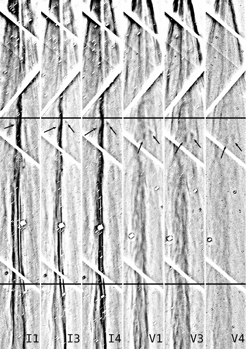
Figure 2: Unsharp masked (highpass50) and 5$\times$5 pixel binned images. The gaps between CCDs are seen in gray. Long exposures, I1, I3, I4, V1, V3 and V4 are displayed from the left to the right. The sun and the nucleus are toward the top. The distance from the nucleus is shown as horizontal lines at 3$\times$10⁵ km and 6$\times$10⁵ km. Two knots are indicated by arrows.

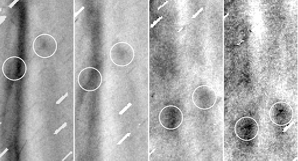
Figure 3: Closeup images around knots. I3, I4, V1, and V3 are displayed from the left to the right. I3 and I4 are highpass50, and V1 and V3 are highpass70 filtered. The positions used in the Figure are indicated with white circles.

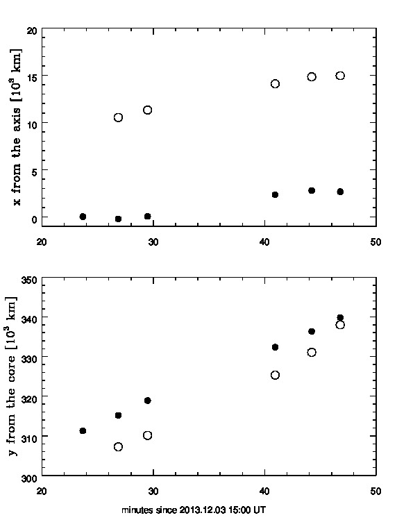
Figure 4: The position of moving knots in Figure 2 and as a function of time. Open and filled symbols correspond to the position of each knot. The top panel shows the tangential distance from the nucleus measured along the tail, and the bottom panel shows the distance from the axis. The abscissa shows the time in minutes since 2013 Dec. 4 at 15:00 UT.

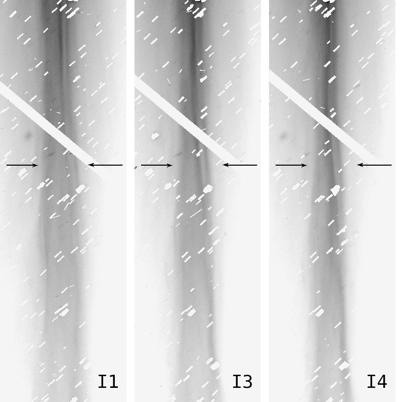
Figure 5: The change in the width of the tail in I-band frames. The images before unsharp masking are shown. The y-positions are shifted assuming a flow of 22 km s^-1. The black arrows show 6$\times$10⁵ km from the nucleus in I1, where the profile is measured (Figure 6).

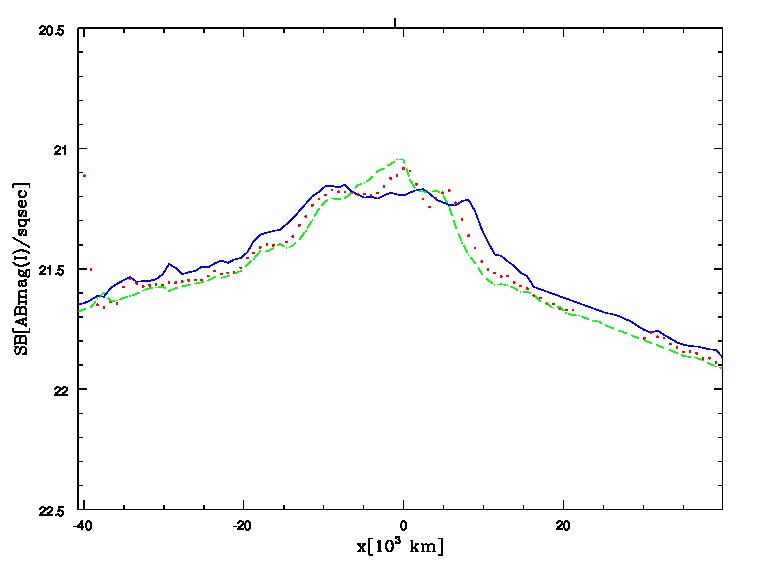
Figure 6: The change in the spatial surface brightness profile across the tail in I-band frames. Blue solid, red dotted and green broken lines corresponds to I1, I3, and I4, respectively. The y-position was 6$\times$10⁵ km from the nucleus in I1, and shifted assuming 22 km s^-1 movement along the tail.

tag	filter	UT(start)	exptime(sec)
I1	I	2013 Dec 4 15:22:41	120.0
I2	I	2013 Dec 4 15:25:10	2.0
I3	I	2013 Dec 4 15:25:51	120.0
I4	I	2013 Dec 4 15:28:29	120.0
V1	V	2013 Dec 4 15:39:57	120.0
V2	V	2013 Dec 4 15:42:33	2.0
V3	V	2013 Dec 4 15:43:14	120.0
V4	V	2013 Dec 4 15:45:43	30.0
V5	V	2013 Dec 4 15:46:43	10.0

Table 1: Observation Log

	JPL#55
epoch	2456653.5 (JD)
q	0.8118255522209098
e	0.9984254232918264
i	64.0409480407445 [deg]
w	67.16643021837888 [deg]
Node	70.7111790783519 [deg]
Tp	2456649.2331241518 (JD)

Table 2: Orbital Elements of C/2013 R1

SDSS-Suprime	SDSS color	range	$c_{0}$	$c_{1}$	$c_{2}$	$c_{3}$	$c_{4}$	$c_{5}$
$g-V$	$g-r$	-0.6$<g-r<$0.8	0.039	0.574	-0.086	0.257	0.188	-0.406
$i-I$	$r-i$	-0.4$<r-i<$0.5	-0.018	0.255	0.037	0.092	-0.196	…

Table 3: The coefficients of color conversion

Appendix A Unsharp masking Procedure

In this study, we first reduced the data following a general data reduction process using nekosoft (Yagi et al., 2002). Figure 7a shows a zoom-up of the area around the the knots in the reduced image of I3. The data consist of background objects (most of them are stars), and cosmic rays as well as the comet tails and their faint substructures. We remove these background objects and cosmic rays in the following way. The non-sidereal tracking generate a characteristic trail of background objects. The direction and length of the trails are determined by the ephemeris that we adopted for the observations with the tracking. To enhance the trails of the background objects for an effective mask generation, we took the difference between two smoothed images, both of which were smoothed with a two-dimensional Gaussian kernel with an elongation perpendicular to the trails, but one with a smaller kernel with the $\sigma$ of $1.5\times 1.0$ pixels and the other with a larger kernel with $5.0\times 2.0$ pixels. This procedure generates a very recognizable pattern around objects that moved according to the adopted ephemeris. Figure 7b shows the pattern, and Figure 7c shows a first mask generated from this image. The background objects are fixed at celestial positions. We therefore shifted the first masks from subsequent exposures and took an ”AND” to make a final mask for all the exposures. The lengths of the trails depend on exposure times, but the mask size would be comparable among the exposures if the exposure time were the same. We made one mask for I-band using (I1, I3, I4), and two masks for V-band using (V1, V3) and (V1, V3, V4) – the first V-band mask was applied for V1 and V3, and the second for V4, since the shorter exposure image has a smaller trail of background objects. An example of masked images is Figure 7d. In Figure 7d, cosmic rays and bad pixels remain unmasked. We then masked pixels whose value is larger than a threshold (Figure 7e). We applied the unshaped masking technique to the images processed above. A result of the unshaped masking with $\sigma=50$ pixels (highpass50) is shown in Figure 7f, which is a part of Figure 2.

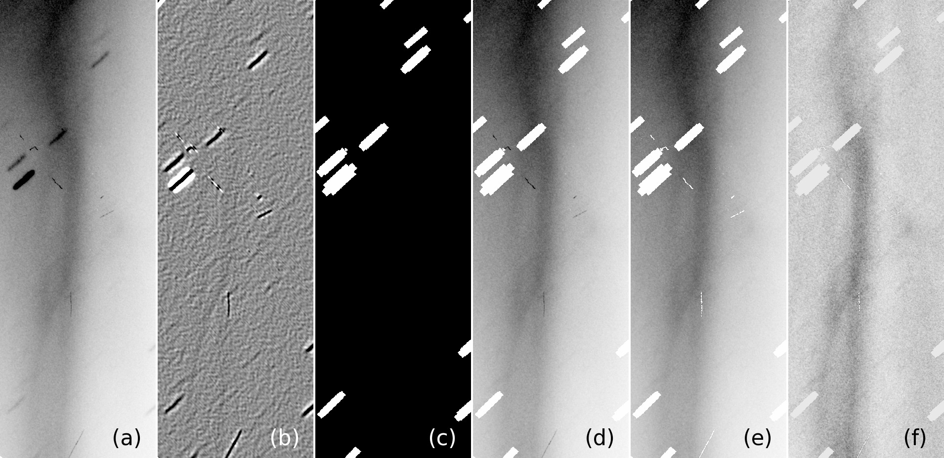
Figure 7: An example of unsharp masking and star-masking process. Cutouts of I3 around the knots are shown. The bright part is shown as black. (a) Image after mosaicking, (b) Enhancement of star trails, (c) Mask pattern made from (b). Mask is shown as white. (d) “AND” mask of I1, I3 and I4. Cosmic rays and cometary structures are removed. (e) Cosmic-rays mask added, (f) Unsharp masked (e), using $\sigma$=50 pixels Gaussian.

Appendix B Tests of detection and measurement with artificial images

To test the reliability of detections of extended structures, we employ tests with images of a fake object. We adopt a circular Gaussian profile with a variety of widths, i.e., $\sigma=$10, 20, 30, 40, 50, and 70 pixels, corresponding to the FWHM of 4.7, 9.5, 14, 19, 24, and 33 arcsec, respectively. We set the peak of the Gaussian to be 70 counts, which is comparable to that of the two knots of interest discussed in Section 3.2. Noise is also added in the artificial images using the double precision SIMD-oriented Fast Mersenne Twister (dSFMT) software .

B.0.1 Effect of noise

We first examined the effect of relatively large noise, with S/N=1 at the peak of the Gaussian profile. In this case, a 5$\times$5 binning improves the S/N to 5 at the peak. We ran SExtractor (Bertin & Alnouts, 1996) for object detection using the 5$\times$5 binned image.

Results are shown in Table 4. The second and third columns show measurements of input models before adding the noise (noise-free). The rest of the columns are for measurements of detected objects using the images with the noise added (noise-added). We generated 1000 random realizations of noise pattern across the images. In some realizations, the Gaussian profile was incorrectly detected as blended objects and was split into multiple objects. In those cases, we summed up the fluxes to calculate a total flux and measured the position of the object using a flux-weighted mean. The FWHM size was not measured in case of the false multiple-object detection. Measured parameters in the two cases, i.e., detections of single and multiple objects are separately shown in Table 4. To estimate errors in FWHM and total flux, we used the median absolute deviation (MAD) and converted the MAD to rms as rms$\sim 1.48\times$ MAD. This is known as a robust estimator of the rms and is valid for the normal distribution.

This test shows that the noise does not largely affect the position measurement in case of single detection; only rms $\sim$ 0.23-0.24 pixels in 5$\times$5 binned image ($\sim$0.2 arcsec). In case of multiple detections the rms of flux-weighted mean position error is up to 0.80 pixels ($\sim$0.8 arcsec). The 0.8 pixel error corresponds to $\sim$ 300 km in this study, which is negligible (see Figure 4). The errors in FWHM and total flux measurements are not negligible. In case of multiple-object detection, the FWHM is about 30-50% larger than the measurements of noise-free models, which is significantly larger than the rms of the measurements. The total flux is smaller by 0.06-0.15 mag in case of single detection, while it is larger by 0.11-0.33 mag in case of multiple detection. These differences are significant except for the $\sigma=$10 model.

The relatively large errors in FWHM and flux measurements may be due to a possible overestimation of the background. We do not investigate the cause of the errors further as the quantitative error estimate given above is enough for this study.

B.0.2 Effect of unsharp masking

We also test errors due to the unsharp masking technique using the noise-added images. Measurements were made with the 5$\times$ 5 binned image after application of the unsharp masking (highpass30, highpass50, and highpass70). We adopted the same 1000 noise realizations as in the previous section.

Results are shown in Table 5–7. If the filter size $\sigma$ is larger than or comparable to a $\sigma$ of Gaussian profile of the fake object, the unsharp-masking technique does not cause large errors in measurements of position and FWHM. The rms of the positional shift is $<$ 0.5 pixels in case of single detection, and $<$ 0.7 pixels in case of multiple detections. The error, i.e., $<$0.7 pixels ($<$300 km), is negligible in this study. The errors in FWHM measurements are comparable before and after the unsharp masking, except for the case of highpass50 with $\sigma=$40. On the other hand, if filter size $\sigma$ is smaller than that of Gaussian of the fake object, the deviation becomes larger and the fraction of no-detection increases.

As expected, the total fluxes measured after the unsharp masking are significantly smaller than those before the masking. The difference is up to 1 mag in the case of single detections and up to 2.4 mag in the case of multiple detections. The large error in flux, however, does not affect the analysis of this paper, since our conclusion is based primarily on positional shifts and corresponding velocities of the clumps. If we adequately select the filter size $\sigma$ with respect to the sizes of the object, the unsharp masking technique works good for positional measurement.

	noise-free		noise-added
					single detection			multiple detection
$\sigma$	FWHM	total	multi.	no	shift rms	FWHM	total	shift rms	total
pixel	pixel	count	det.	det.	pixel	pixel	count	pixel	count
10	4.7	1800	4	0	0.23	7$\pm$1	1700 $\pm$200	0.26	2000$\pm$ 200
20	9.4	7000	95	0	0.23	13$\pm$1	6500 $\pm$300	0.38	9500$\pm$ 1000
30	14	15800	148	0	0.23	20$\pm$1	14300 $\pm$500	0.47	21300$\pm$ 1900
40	19	28100	135	0	0.24	26$\pm$1	25100 $\pm$800	0.57	37600$\pm$ 3000
50	24	43900	123	0	0.24	32$\pm$1	38800 $\pm$1000	0.71	57000$\pm$ 5500
70	33	85900	78	0	0.24	44$\pm$1	74700 $\pm$1700	0.80	105500$\pm$ 15200

Table 4: Measurement of artificial objects

	highpass30
			single detection			multiple detection
$\sigma$	multiple	no detection	shift rms	FWHM	total	shift rms	total
pixel			pixel	pixel	count	pixel	count
10	1	0	0.24	7$\pm$ 1	1200$\pm$ 100	0.40	1200
20	61	0	0.30	12$\pm$ 1	2600$\pm$ 200	0.44	3400$\pm$ 400
30	153	0	0.50	11$\pm$ 2	3100$\pm$ 300	0.52	4600$\pm$ 600
40	113	181	1.01	8$\pm$ 2	2700$\pm$ 600	0.85	4200$\pm$ 700
50	14	825	1.62	7$\pm$ 2	2100$\pm$ 600	1.16	3500$\pm$ 600
70	1	996	3.94	8$\pm$ 3	700$\pm$ 300	2.90	1500

Table 5: Measurement of unsharp-masked artificial objects

	highpass50
			single detection			multiple detection
$\sigma$	multiple	no detection	shift rms	FWHM	total	shift rms	total
pixel			pixel	pixel	count	pixel	count
10	0	0	0.23	7$\pm$ 1	1400$\pm$ 100	…	…
20	102	0	0.24	13$\pm$ 1	4300$\pm$ 200	0.37	5700$\pm$ 500
30	264	0	0.28	18$\pm$ 2	6900$\pm$ 400	0.52	9700$\pm$ 1300
40	427	0	0.36	18$\pm$ 3	8400$\pm$ 500	0.45	13300$\pm$ 1900
50	589	0	0.48	15$\pm$ 4	9100$\pm$ 900	0.56	14900$\pm$ 2800
70	367	23	1.98	8$\pm$ 2	4100$\pm$ 1500	1.38	7700$\pm$ 2200

Table 6: Measurement of unsharp-masked artificial objects

	highpass70
			single detection			multiple detection
$\sigma$	multiple	no detection	shift rms	FWHM	total	shift rms	total
pixel			pixel	pixel	count	pixel	count
10	0	0	0.23	7$\pm$ 1	1600$\pm$ 100	…	…
20	110	0	0.24	13$\pm$ 1	5200$\pm$ 300	0.38	7200$\pm$ 600
30	242	0	0.25	19$\pm$ 2	9600$\pm$ 400	0.42	13400$\pm$ 1900
40	400	0	0.28	25$\pm$ 2	13500$\pm$ 600	0.55	20300$\pm$ 3500
50	588	0	0.33	27$\pm$ 2	16300$\pm$ 100	0.66	26700$\pm$ 5100
70	871	0	0.47	22$\pm$ 4	18400$\pm$ 1800	0.70	31900$\pm$ 6600

Table 7: Measurement of unsharp-masked artificial objects

References

- Aihara et al. (2011) Aihara, H., Allende, P., An, D. et al. 2011, ApJS, 193, 29
- Bertin & Alnouts (1996) Bertin, E., Alnoults, S. 1996, A&A, 117, 393
- Blanton & Roweis (2007) Blanton, M.R., Roweis, S. 2007, AJ, 133, 734
- Brandt et al. (2002) Brandt, J.C., Snow, M., Yi, Y. et al. 2002, Earth Moon Planets, 90, 15
- Buffington et al. (2008) Buffington, A. et al. 2008, ApJ, 677, 798
- Downs et al. (2013) Downs, C., Linker, J.A., Mikić, Z., et al. 2013, Science, 340, 1196
- Iye et al. (2004) Iye, M., Karoji, H., Ando, H. et al. 2004, PASJ, 56, 381
- Kinoshita et al. (1996) Kinoshita, D., Fukushima, H., Watanabe, J.-I., Yamamoto, N. 1996, PASJ, 48, L83
- Lasker et al. (2008) Lasker, B.M., Lattanzi, M.G., McLean, B.J. et al. 2008, AJ, 136, 735
- Miyazaki et al. (2002) Miyazaki, S., Komiyama, Y., Sekiguchi, M. et al. 2002, PASJ, 54, 833
- Mendis (2006) Mendis, D.A. 2006, in Recurrent Magnetic Storms: Corotating SolarWind, ed. B. T. Tsurutani et al. (Geophysical Monograph Series, Vol. 167; Washington, DC: AGU), 31
- Niedner (1981) Niedner, M.B. Jr. 1981, ApJS, 46, 141
- Niedner (1982) Niedner, M.B. Jr. 1982, ApJS, 48, 1
- Saito et al. (1987) Saito, T., Yumoto, K., Hirao, K. et al. 1987, A&A, 187, 209
- Yagi et al. (2002) Yagi, M., Kashikawa, N., Sekiguchi, M. 2002, AJ, 123, 66
- Yagi (2012) Yagi, M. 2012, PASP, 124, 1347
- Yagi et al. (2013) Yagi, M., Suzuki, N., Yamanoi, H. et al. 2013, PASJ, 65, 22