Integer Programming Relaxations for Integrated Clustering and Outlier Detection

Abstract

In this paper we present methods for exemplar based clustering with outlier selection based on the facility location formulation. Given a distance function and the number of outliers to be found, the methods automatically determine the number of clusters and outliers. We formulate the problem as an integer program to which we present relaxations that allow for solutions that scale to large data sets. The advantages of combining clustering and outlier selection include: (i) the resulting clusters tend to be compact and semantically coherent (ii) the clusters are more robust against data perturbations and (iii) the outliers are contextualised by the clusters and more interpretable, i.e. it is easier to distinguish between outliers which are the result of data errors from those that may be indicative of a new pattern emergent in the data. We present and contrast three relaxations to the integer program formulation: (i) a linear programming formulation (LP) (ii) an extension of affinity propagation to outlier detection (APOC) and (iii) a Lagrangian duality based formulation (LD). Evaluation on synthetic as well as real data shows the quality and scalability of these different methods.

1 Introduction

Figure 1: Clustering results for a 2D dataset with $k=10$, $100$ points per cluster and $100$ outliers. APOC and LD accurately detect the clusters and select appropriate outliers without requiring $k$ as input. k-means–, provided with the correct value of $k$, fails to split certain clusters which results in the selection of non-outliers as outliers. Black crosses indicate the outliers selected, points of identical colour indicate clusters and the red circles indicate errors made by k-means–.

Clustering and outlier detection are often studied and investigated as two separate problems (Chandola et al., 2009). However, it is natural to consider them simultaneously. For example, outliers can have a disproportionate impact on the location and shape of clusters which in turn can help identify, contextualise and interpret the outliers.

A branch of statistics known as “robust statistics” studies the design of statistical methods which are less sensitive to the presence of outliers (Huber and Ronchetti, 2008). For example, the median and trimmed mean estimators are far less sensitive to outliers than the mean. Similarly, versions of Principal Component Analysis (PCA) have been proposed (Croux and Ruiz-Gazen, 1996; Wright et al., 2009) which are more robust against model mis-specification. An important primitive in the area of robust statistics is the notion of Minimum Covariance Determinant (MCD): Given a set of $n$ multivariate data points and a parameter $\ell$, the objective is to identify a subset of points which minimises the determinant of the variance-covariance matrix over all subsets of size $n-\ell$. The resulting variance-covariance matrix can be integrated into the Mahalanobis distance and used as part of a chi-square test to identify multivariate outliers (Rousseeuw and Driessen, 1999).

In the theoretical computer science literature, similar problems have been studied in the context of clustering and facility location. For example, Chen (2008) has considered and proposed a constant factor approximation algorithm for the k-median with outliers problem: Given $n$ data points and parameters $k$ and $\ell$, the objective is to remove a set of $\ell$ points such that the cost of k-median clustering on the remaining $n-\ell$ points is minimised. Earlier Charikar et al. (2001), have proposed a bi-criteria approximation algorithm for the facility location with outliers problem. While of theoretical interest, none of these algorithms are amenable to a practical implementation on large data sets.

Robustness of clustering methods in general is discussed in (Garc a-Escudero et al., 2010; Hennig, 2008). They provide a good theoretical overview about the conditions under which clustering methods can deal with noise or outliers. However, it is difficult to determine a-priori if data exhibits the required properties.

More recently, Chawla and Gionis (2013) have proposed $k$-means– a practical and scalable algorithm for the k-means with outlier problem. k-means– is a simple extension of the $k$-means algorithm and is guaranteed to converge to a local optima. However, the algorithm inherits the weaknesses of the classical $k$-means algorithm. These are: (i) the requirement of setting the number of clusters $k$ and (ii) initial specification of the $k$ centroids. It is well known that the choice of $k$ and initial set of centroids can have a large impact on the result. Trimmed $k$-means (Cuesta-Albertos et al., 1997) is a special case of k-means– with $k=1$.

In this paper we present methods that approach the problem of joint clustering and outlier detection as an integer programming optimisation task. The resulting algorithms find the number of cluster on their own and require as sole input the distance between pairs of points as well as the number $\ell$ of outliers to select. We propose three methods to solve this, each with their benefits and drawbacks: (i) affinity propagation (Frey and Dueck, 2007) extension to outlier detection, (ii) linear programming and (iii) Lagrangian duality relaxation. The main contributions of the paper are as follows:

• formulation of the clustering with outlier detection problem as an integer program;

• modification of the affinity propagation model and derivation of new update rules;

• scalable algorithm based on Lagrangian duality;

• approximation analysis of real data based on linear programming solutions;

• evaluation on synthetic and real-world data sets.

The remainder of the paper is structured as follows. In problem-formulation we describe the problem in detail. Following that in methods we describe the different methods. In experiments we evaluate the methods on both synthetic and real datasets. related-work provides some additional information on related work before we conclude in conclusion.

2 Problem Formulation

Given the assignment cost matrix $d_{ij}$ and cluster creation costs $c_{i}$ we define the task of clustering and outlier selection as the problem of finding the assignments to the binary exemplar indicators $y_{i}$, outlier indicators $o_{i}$ and point assignments $x_{ij}$ that minimises the following energy function:

$$\min\sum_{i}c_{i}y_{i}+\sum_{i}\sum_{x}d_{ij}x_{ij},$$ (1)

subject to

$$x_{ij} \leq y_{j}$$ (2)

$$o_{i}+\sum_{j}x_{ij} =1$$ (3)

$$\sum_{i}o_{i} =\ell$$ (4)

$$x_{ij},y_{j},o_{i} \in\{0,1\}.$$ (5)

In order to obtain a valid solution a set of constraints have been imposed:

• points can only be assigned to valid exemplars ip-c-1

• every point must be assigned to exactly one other point or declared an outlier ip-c-2

• exactly $\ell$ outliers have to be selected ip-c-3

• only integer solutions are allowed ip-c-4

These constraints describe the facility location problem with outlier selection (FLO). This allows the algorithm to select the number of clusters automatically and implicitly defines outliers as those points whose presence in the dataset has the biggest negative impact on the overall solution.

In the following we explore three different methods of formulating and solving the above generic problem. In the experiments we evaluate each of the methods under different criteria such as quality of the solution, complexity of the method and applicability to large datasets

3 Methods

In the following we will describe three ways of solving the problem stated in problem-formulation. We start with a linear programming formulation which is known to provide the optimal answer if the solution is integer. Next we propose an extension to affinity propagation which is a conceptually nice method. Finally, we propose a method based on Lagrangian duality which is highly scalable while achieving results very close to the optimum found by LP.

3.1 Linear Programming Relaxation

The first method we present is based on linear programming and will serve as ground truth for the other two methods. In order to solve the integer program described in problem-formulation we have to relax it. If the solution to this relaxed formulation is integer, i.e. all assignments are either $0$ or $1$, we have found the optimal solution. The relaxed linear program has the following form:

$$\min\sum_{i}\sum_{j}x_{ij}d_{ij}$$ (6)

subject to

$$x_{ij} \leq x_{ii}$$ (7)

$$\sum_{j}x_{ij}+\sum_{k}o_{ik} =1$$ (8)

$$\sum_{i}o_{ik} =1$$ (9)

$$0\leq x_{ij},o_{ik}\leq 1 \hskip 14.22636pt\forall i,j,k$$ (10)

where $d_{ij}$ is again the distance between point $i$ and $j$. This follows Komodakis et al. (2008) with additional constraints to enforce the outlier selection. We note here that lp-energy uses the diagonal to indicate exemplar selection as it maps more easily to affinity propagation. The constraint in lp-c-1 enforces the condition that points are only assigned to valid exemplars. lp-c-2 enforces that a point is either assigned to a single cluster or is declared as an outlier. lp-c-3 ensures that every outlier point is used exactly once thus enforcing that exactly $\ell$ outliers are selected. Finally, lp-c-4 is the relaxation of the original integer program.

3.2 Affinity Propagation Outlier Clustering

The extension to affinity propagation, based on the binary variable model (Givoni and Frey, 2009), solves the integer program of problem-formulation by representing it as a factor graph, shown in apoc-model. This factor graph is solved using belief propagation and is based on the following energy function:

$$\max\sum_{ij}S_{ij}(x_{ij})+\sum_{j}E_{j}(x_{:j})+\sum_{i}I_{i}(x_{i:},o_{i:})+\sum_{k}P_{k}(o_{:k}),$$ (11)

where

$$S_{ij}(x_{ij}) =\begin{cases}-c_{i}&\text{if }i=j\\ -d_{ij}&\text{otherwise}\end{cases}$$ (12)

$$I_{i}(x_{i:},o_{i:}) =\begin{cases}0&\text{if }\sum_{j}x_{ij}+\sum_{k}o_{ik}=1\\ -\infty&\text{otherwise}\end{cases}$$ (13)

$$E_{j}(x_{:j}) =\begin{cases}0&\text{if }x_{jj}=\max_{i}c_{ij}\\ -\infty&\text{otherwise}\end{cases}$$ (14)

$$P_{k}(o_{:k}) =\begin{cases}0&\text{if }\sum_{i}o_{ik}=1\\ -\infty&\text{otherwise}\end{cases}$$ (15)

with $x_{i:}=x_{i1},\dots,x_{iN}$. Since we use the max-sum algorithm we maximise the energy function and use negative distances. The three constraints can be interpreted as follows:

1. 1-of-$N$ Constraint ($I_{i}$). Each data point has to choose exactly one exemplar or be declared as an outlier.

2. Exemplar Consistency Constraint ($E_{j}$). For point $i$ to select point $j$ as its exemplar, point $j$ must declare itself an exemplar.

3. Select $\ell$ Outliers Constraint ($P_{k}$). For every outlier selection exactly one point is assigned.

These constraints are enforced by associating an infinite cost with invalid configurations,thus resulting in an obviously suboptimal solution.

Figure 2: Graphical model of APOC. The left part is responsible for the clustering of the data, while the right part is responsible for the outlier selection. These two parts interact with each other via the $I$ factor nodes.

Figure 3: Messages exchanged by the APOC graphical model. $x_{ij}$ represents the clustering choice whereas $o_{ik}$ represents the outlier choice.

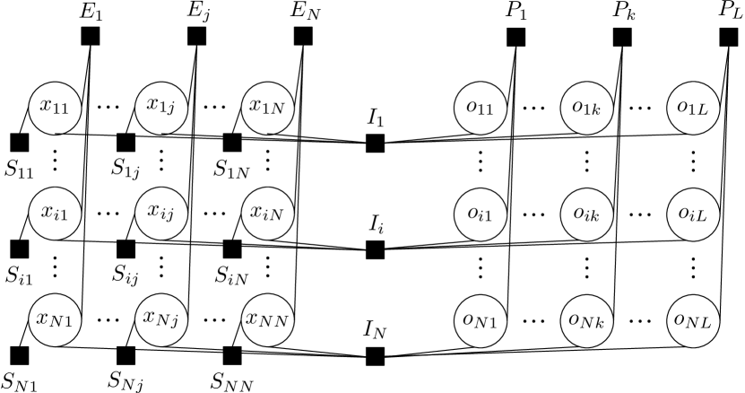
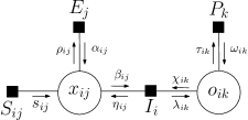
The energy function is optimised with the max-sum algorithm (Kschischang et al., 2001), which allows the recovery of the maximum a posteriori (MAP) assignments of the $x_{ij}$ and $o_{ik}$ variables. The algorithm works by exchanging messages between nodes in the factor graph. In their most general form these messages are defined as follows:

$$\mu_{v\rightarrow f}(x_{v}) =\sum_{f^{*}\in ne(v)\setminus f}\mu_{f^{*}\rightarrow v}(x_{v}),$$ (16)

$$\begin{split}\mu_{f\rightarrow v}(x_{v})&=\max_{x_{1},\dots,x_{M}}\Big{[}f(x_{v},x_{1},\dots,x_{M})\\ &+\sum_{v^{*}\in ne(f)\setminus v}\mu_{v^{*}\rightarrow f}(x_{v^{*}})\Big{]},\end{split}$$ (17)

where $\mu_{v\rightarrow f}(x)$ is the message sent from node $v$ to factor $f$, $\mu_{f\rightarrow v}(x_{v})$ is the message from factor $f$ sent to node $v$, $ne()$ is the set of neighbours of the given factor or node and $x_{v}$ is the value of node $v$.

The messages exchanged by APOC are shown in apoc-messages. We can see that each node $x_{ij}$ is connected to three factors: $S_{ij}$, $I_{i}$ and $E_{j}$ whereas outlier nodes $o_{ik}$ are connected to only two, $I_{i}$ and $P_{k}$. Messages $\rho_{ij}$, $\beta_{ij}$, $\tau_{ik}$ and $\xi_{ik}$ are sent from nodes to factors and derived using mp-nf. The other five messages $s_{ij},\alpha_{ij}$, $\eta_{ij}$, $\lambda_{ik}$ and $\omega_{ik}$ are derived with mp-fn since they are sent from a factor to a node. Since only binary variables are involved it is sufficient to compute the difference between the two variable settings. Combining these messages we obtain the final set of update equations as:

$$\rho_{ij} =s_{ij}+\min\left[-\max_{t\neq j}(\alpha_{it}+s_{it}),-\max_{t}(\omega_{it})\right]$$ (18)

$$\alpha_{ij} =\begin{cases}\sum_{t\neq j}\max(0,\rho_{tj})&i=j\\ \min\left[0,\rho_{jj}+\sum_{t\notin\{i,j\}}\max(0,\rho_{tj})\right]&i\neq j\end{cases}$$ (19)

$$\lambda_{ik} =\min\left[-\max_{t}(\alpha_{it}+s_{it}),-\max_{t\neq k}(\omega_{ti})\right]$$ (20)

$$\omega_{ik} =-\max_{t\neq i}(\lambda_{tk})$$ (21)

The above equations show how to update the messages, however, we still need to explain how to initialise the messages, determine convergence and extract the MAP solution. First, it is important to set the diagonal entries of $S$ properly. Typically using $S_{ii}=\theta*median(S)$ is a good choice, with $\theta\in[1,30]$. The messages $\alpha_{ij},\rho_{ij}$ and $\lambda_{ik}$ are initialised to $0$ and $\omega_{ik}$ to the median of $S$. Once the messages are initialised we update them in turn with damping until we achieve convergence. Convergence is achieved when the energy of the solution is not changing drastically over a few iterations. The outliers are determined as the $\ell$ points with the largest values of $\max_{k}(\lambda_{ik}+\omega_{ik})$. From the remaining points the exemplars are then selected as the points for which $(\alpha_{ii}+\rho_{ii})>0$ is true. All other points $i$ are assigned to the exemplar $e$ satisfying $\operatorname*{\arg\,\max}_{e}(\alpha_{ie}+\rho_{ie})$. This entire process is shown in apoc-algo, where we first initialise the messages, then update them until convergence and finally extract the MAP solution.

1

2foreach $i,j\in\{1,\dots,N$} do

3       $\alpha_{ij}\leftarrow 0$;

4       $\rho_{ij}\leftarrow 0$;

5      

6 end foreach

7foreach $i\in\{1,\dots,N\},k\in\{1,\dots,\ell\}$ do

8       $\lambda_{ik}\leftarrow 0$;

9       $\omega_{ik}\leftarrow\text{median}(S)$;

10      

11 end foreach

12

13repeat

14       update $\rho$ according to apoc_rho;

15       update $\alpha$ according to apoc_alpha;

16       update $\lambda$ according to apoc_lambda;

17       update $\omega$ according to apoc_omega;

18      

19until convergence;

20$O\leftarrow$ extract outliers;

21 $E\leftarrow$ extract exemplars;

22 $A\leftarrow$ find exemplar assignments;

Algorithm 1 $\text{apoc}(S,\ell)$

3.3 Lagrangian Duality

The final method is based on Lagrangian duality. The basic idea is to relax the original problem by introducing Lagrange multipliers $\lambda$. The result is a dual problem which is now concave with a unique maximum, making it possible to use gradient ascent based methods. However, the resulting function is not differentiable and requires the use of subgradients.

We restate the original problem here for convenience:

$$\min\sum_{j}y_{j}c_{j}+\sum_{i}\sum_{j}x_{ij}d_{ij}$$ (22)

subject to

$$x_{ij} \leq y_{j}$$ (23)

$$o_{i}+\sum_{j}x_{ij} =1$$ (24)

$$\sum_{i}o_{i} =\ell$$ (25)

$$0\leq x_{ij},y_{j},o_{i}\leq 1 \hskip 14.22636pt\forall i,j,$$ (26)

where $o_{i}=1$ indicates that point $i$ is an outlier and $\ell$ is the number of outliers we wish to find. ld-c-1 encodes that a point can only be assigned to a valid exemplar. The second constraint ld-c-2 enforces that a point is either assigned to a single cluster or selected as an outlier. The final constraint, ld-c-3, ensures that exactly $\ell$ outliers are selected. Relaxing ld-c-2 yields:

$$\min\underbrace{\sum_{i}(1-o_{i})\lambda_{i}}_{\text{outliers}}+\underbrace{\sum_{j}c_{j}y_{j}+\sum_{i}\sum_{j}(d_{ij}-\lambda_{i})x_{ij}}_{\text{clustering}}.$$ (27)

subject to

$$x_{ij} \leq y_{i}$$ (28)

$$\sum_{k}o_{k} =\ell$$ (29)

$$0\leq x_{ij},y_{j},o_{k}\leq 1 \hskip 14.22636pt\forall i,j,k$$ (30)

We now solve this relaxed problem using the idea of Bertsimas and Weismantel (2005) by finding valid assignments that attempt to minimise ld-relaxed without optimality guarantees. The Lagrange multipliers $\lambda$ act as a penalty incurred for constraint violation which we try to minimise. From ld-relaxed we see that the penalty influences two parts: outlier selection and clustering. We select good outliers by designating the $\ell$ points with largest $\lambda$ as outliers, as this removes a large part of the penalty. For the remaining $N-\ell$ points we determine clustering assignments by setting $x_{ij}=0$ for all pairs for which $d_{ij}-\lambda_{i}\geq 0$. To select the exemplars we compute

$$\mu_{j}=c_{j}+\sum_{i:d_{ij}-\lambda_{i}<0}(d_{ij}-\lambda_{i}),$$ (31)

which represents the amortised cost of selecting point $j$ as exemplar and assigning points to it. Thus, if $\mu_{j}<0$ we select point $j$ as an exemplar and set $y_{j}=1$, otherwise we set $y_{j}=0$. Finally, we set $x_{ij}=y_{j}$ if $d_{ij}-\lambda_{i}<0$. From this complete assignment we then compute a new subgradient $\mathbf{s}^{t}$ and update the Lagrangian multipliers $\lambda^{t}$ as follows:

$$\mathbf{s}_{j}^{t} =1-\sum_{j}x_{ij}$$ (32)

$$\lambda_{j}^{t} =\max(\lambda_{j}^{t-1}+\theta^{t}\mathbf{s}_{j},0),$$ (33)

where $\theta^{t}$ is the step size at time $t$ computed as

$$\theta^{t}=\theta^{0}\>\text{pow}(\alpha,t)\quad\alpha\in(0,1),$$ (34)

where $\text{pow}(a,b)=a^{b}$. To obtain the final solution we repeat the above steps until the changes become small enough, at which point we extract a feasible solution. This is guaranteed to converge (Bertsimas and Weismantel, 2005) if a step function is used for which the following holds:

$$\sum_{t=1}^{\infty}\phi_{t}=\infty\qquad\text{and}\qquad\lim_{t\rightarrow\infty}\theta_{t}=0.$$ (35)

3.3.1 Scalable Implementation Considerations

In order to enable the algorithm to scale to large datasets we have to consider the limited availability of main memory. First we cannot assume that the complete distance matrix can fit into main memory. Therefore, we compute the distances on the fly. Since this involves $N^{2}$ evaluations per iteration it is the most costly part of the method. However, the evaluation of the distance function can be easily parallelised. In practice with simple distance functions, such as the Euclidean distance, approximately 75% of the computational time is spent evaluating the distance function. Another important point is that just as storing the full distance matrix is not possible, neither is storing the full assignment matrix $\mathbf{x}$. However, we are only interested in the values where $x_{ij}=1$, which is a small portion of the full matrix. Thus we can use standard sparse matrix implementations to manage the assignment matrix.

The pseudo code in ld-algo shows how to compute the assignment matrix $\mathbf{x}$ using the above mentioned improvements. Lines 1 through 5 initialise the required storage. In lines 6 to 12 we sort the points in descending order according to their $\lambda$ values, by first creating pairs of point index and value and then sorting these. The computationally intensive but also parallelisable part of the algorithm is located in lines 13 to 21. There we compute the exemplar score $\mu_{j}$ and at the same time remember point pairs $(i,j)$ for which $d_{ij}-\lambda_{i}<0$. Lines 22 to 27 then perform the exemplar assignments based on $\mu_{j}$. Finally, in lines 28 to 31 we set the assignment $x_{ij}=1$ if $y_{j}=1$. Lastly, we return assignments, exemplars and outliers.

1

2

$\mathcal{O}\leftarrow\mathbf{0}$;

  // Outlier indicators

$\mathbf{y}\leftarrow\mathbf{0}$;

  // Exemplar indicators

$\mathcal{L}\leftarrow\emptyset$;

  // Set of $(i,\lambda_{i})$ pairs

$\mathcal{S}\leftarrow\emptyset$;

  // Assignment pairs $(i,j)$

$\mathbf{x}\leftarrow\mathbf{0}$;

  // Assignments

3

// Selecting outliers

4 foreach $i\in\{1,\dots,N\}$ do

5       $\mathcal{L}\leftarrow\mathcal{L}\cup(i,\lambda_{i})$;

6 end foreach

7$\mathcal{L}\leftarrow sort(\mathcal{L})$;

8 foreach $i\in\{1,\dots,L\}$ do

9       $\mathbf{\mathcal{missing}}O_{\mathcal{L}_{i,1}}\leftarrow 1$;

10      

11 end foreach

12

// Compute exemplar and outlier scores

13 foreach $j\in\{1,\dots,N$} do

14       $\mu_{j}\leftarrow c_{j}$;

15       foreach $i\in\{1,\dots,N$} do

16             $q\leftarrow dist(i,j)-\lambda_{i}$;

17             if $q<0$ then

18                   $\mu_{j}\leftarrow\mu_{j}+q$;

19                   $\mathcal{S}\leftarrow\mathcal{S}\cup(i,j)$;

20                  

21            

22       end foreach

23      

24 end foreach

25

// Select exemplars

26 foreach $j\in\{1,\dots,N$} do

27       if $\mu_{j}<0$ then

28             $\mathbf{y}_{j}\leftarrow 1$;

29            

30      else

31             $\mathbf{y}_{j}\leftarrow 0$;

32            

33       end if

34      

35 end foreach

36

// Perform cluster assignments

37 foreach $s\in\mathcal{S}$ do

38       if $\mu_{s_{2}}=1$ then

39             $x_{p_{1},p_{2}}\leftarrow 1$;

40            

41       end if

42      

43 end foreach

44

45return $\mathbf{x},\mathbf{y},\mathcal{O}$;

Algorithm 2 $\text{LD-Iteration}(\lambda)$

3.4 Comparisons

Now that we have presented the different methods we want to give an overview of the advantages and disadvantages of these. method-comparison presents a quick overview of different properties of the proposed methods discussed in more detail next. First, the speed of APOC and LD clearly outperform LP by a large margin, however, other methods such as k-means– still perform better.

With regards to optimality we know that

$$FLO_{LP}\penalty 0\leq FLO_{LD}\leq FLO_{IP}$$ (36)

(Bertsimas and Weismantel, 2005). Additionally, if LP finds a solution that is integer it is equivalent to the IP one, i.e. $FLO_{LP}=FLO_{IP}$. In the experiments we see that even though LP finds the optimal solution, LD fails to do so. This contradicts theory, but is explained by the fact that for performance gains we sacrifice some optimality. More specifically, we use discounted updates of the solution matrix $\mathbf{x}$ as well as stop before we converge to a pure integer solution. APOC has no theoretical guarantees on either convergence or optimality bounds of the solution. While such guarantees can be given for certain types of structures with belief propagation (Weiss et al., 2007) it is unclear how they apply to the special case of APOC. However, in practice both APOC and LD achieve scores very close to the optimum.

The speed of LP clearly makes it impossible to scale for large datasets which leaves us with the comparison of APOC and LD. APOC requires storage for messages and similarities and operations which cannot be supported by standard sparse matrix implementations. As such APOC cannot be made truly scalable. LD on the other hand spends the majority of its runtime computing distances between pairs of points, a task that can easily be parallelised. Furthermore the actual assignment matrix can easily be stored using standard sparse matrix implementations. Thus LD is a much better candidate for large scale datasets. Finally, with regards to extensibility LP is the easiest as the relaxation only touches the variables. LD is more involved as there is more freedom in the relaxation of the constraints and a way to solve the dual problem efficiently has to be devised. Affinity propagation is the hardest one as it requires very careful choice of constraints which can be modelled by the graphical model and laborious derivation of update rules, which makes it much harder to come up with solutions to new problems.

Table 1: Advantages and disadvantages of LP, APOC and LD. See method-comparison for detailed explanation.

	LP	APOC	LD
Speed	$--$	$+$	$+$
Optimality	$++$	$+$	$+$
Scalability	$--$	$-$	$+$
Extensibility	$++$	$-$	$+$

4 Experiments

In this section the proposed methods are evaluated on both synthetic and real data. We first present experiments using synthetic data to show different properties of the presented methods and a quantitative analysis. We then process GPS traces of hurricanes to show the applicability of this method to real data. Finally, we present results on two image datasets visually showing the quality of the clusters and outliers found.

Both APOC and LD require a cost for creating clusters. In all experiments we obtain this value as $\theta*\text{median}(x_{ij})$, i.e. the median of all distances multiplied by a scaling factor $\theta$ which is typically in the range $[1,30]$.

4.1 Synthetic Data

We use synthetic datasets to evaluate the performance of the proposed methods in a controlled setting. We randomly sample $k$ clusters with $m$ points each from $d$-dimensional normal distributions $\mathcal{N}(\mu,\Sigma)$ with randomly selected $\mu$ and $\Sigma$. To these clusters we add $\ell$ additional outlier points that have a low probability of belonging to any of the selected clusters.

We compare APOC and LD against k-means– using k-means++ (Arthur and Vassilvitskii, 2007) to select the initial centres. Euclidean distance is used as the metric for all methods. Unless mentioned otherwise k-means– is provided with the exact number of clusters generated, while APOC and LD are required to determine this automatically.

To assess the performance of the methods we use the following three metrics:

1. Normalised Jaccard index, measures how accurately a method selects the ground truth outliers. It is a coefficient computed between selected outliers $O$ and ground-truth outliers $O^{*}$. The final coefficient is normalised with regards to the best possible coefficient obtainable in the following way:

   $$J(O,O^{*})=\frac{|O\cap O^{*}|}{|O\cup O^{*}|}/\frac{\min(|O|,|O^{*}|)}{\max(|O|,|O^{*}|)}.$$ (37)

2. Local outlier factor (Breunig et al., 2000) (LOF) measures the outlier quality of a point. We compute the ratio between the average LOF of $O$ and $O^{*}$, which indicates the quality of the set of selected outliers.

3. V-Measure (Rosenberg and Hirschberg, 2007) indicates the quality of the overall clustering solution. The outliers are considered as an additional class for this measure.

For all the metrics a value of 1 is the optimal outcome.

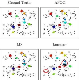
In synth-2d-example we present clustering results obtained by the different methods. Both APOC and LD manage to identify the correct number of clusters and select accurate outliers. k-means– on the other hand, even with good initialisation and correct value for $k$ specified, fails to find the correct clusters and as a result finds a suboptimal solution. The errors made by k-means– are highlighted by the red circles.

Figure 4: The impact of increasing the data dimensionality on the quality of the clustering and outlier selection quality. APOC and LD provide similar results while k-means–, provided with the correct $k$, has more trouble.

We first investigate the influence of the data dimensionality on the results. From synth-dimensions it is clear that in general the quality of the solution increases with higher dimensions. This can be explained by the fact that in higher dimensional spaces the points are farther apart and hence easier to cluster. Looking at k-means– we can see that it struggles more then the other two methods even though it is provided with the correct number of clusters. In higher dimensions it achieves perfect scores for the two outlier centric measures but is unable to always find the correct solution to the whole clustering problem. Looking at APOC and LD we can see that both have little trouble finding perfect solutions in high dimensions. In lower dimensions LD shows a bit more variability compared to APOC. In general, the two dimensional data is the most challenging one and thus will be used for all further experiments.

The number of outliers $\ell$ is a parameter that all methods require. Typically the correct value of $\ell$ is unknown and it is therefore important to know how the algorithms react when the user’s estimate is incorrect. We generate 2D datasets with 2000 inliers and 200 outliers and vary the number of outliers $\ell$ selected by the methods. The results in synth-outliers show that in general no method breaks completely if the correct value for $\ell$ is not provided. Looking at the Jaccard index we see that if $\ell$ is smaller then the true number of outliers all methods pick only outliers. When $\ell$ is greater then the true number of outliers we can see a difference in performance, namely that LD picks the largest outliers which APOC does to some extent as well, while k-means– does not seem to be very specific about which points to select. This difference in behaviours stems from the fact that APOC and LD optimise a cost function in which removing the biggest outliers is the most beneficial. The LOF ratio shows a similar picture as the Jaccard index. For $\ell=100$ the values are much lower as not all outliers can be picked. For the other cases APOC and LD perform similarly while k-means– shows higher variability. Finally, V-Measure shows that the overall clustering results remain accurate even if the number of outliers is misspecified. For large differences between actual and specified outliers a drop in clustering performance can be observed.

Figure 5: The impact of number of outliers specified ($\ell$) on the quality of the clustering and outlier detection performance. APOC and LD perform similarly with more stability and better outlier choices compared to k-means–. We can see that overestimating $\ell$ is more detrimental to the overall performance, as indicated by the LOF Ratio and V-Measure, then underestimating it.

(a) Speedup over LP

(b) Total Runtime

(c) Time per Iteration

Figure 6: The graphs shows how the number of points influences different measures. In (a) we compare the speedup of both APOC and LD over LP. (b) compares the total runtime needed to solve the clustering problem for APOC and LD. Finally, (c) plots the time required (on a log scale) for a single iteration for APOC and LD.

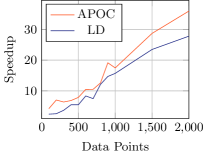
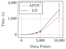
Since both APOC and LD are not guaranteed to find the optimal solution we investigate how close the solutions obtained are to the optimum. The ground truth needed for this is obtained by solving the LP formulation of lp with CPLEX. This comparison indicates what quality can be typically expected from the two methods. Additionally, we can evaluate the speed of these approximations. We evaluate 100 datasets, consisting of 2D Gaussian clusters and outliers, with varying number of points. On average APOC obtains an energy that is $96\%\pm 4\%$ of the optimal solution found by LP, LD obtains $94\%\pm 5\%$ of the LP energy while k-means–, with correct k, only obtains $86\%\pm 12\%$ of the optimum. These results reinforce the previous analysis; APOC and LD perform similarly while outperforming k-means–. We now look at the speedup of APOC and LD over LP, as shown in lp-ld-apoc-comparisons a). Both methods outperform LP by a large margin which only grows the more points are involved. Overall for a small price in quality the two methods obtain a solution significantly faster.

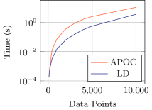
Next we compare the performance between APOC and LD. lp-ld-apoc-comparisons b) shows the overall runtime of both methods for varying number of data points. Here we observe that APOC takes less time then LD. However, by observing the time a single iteration takes, shown in lp-ld-apoc-comparisons c), we see that LD is much faster on a per iteration basis compared to APOC. In practice LD requires several times the number of iterations of APOC, which is affected by the step size function used. Using a more sophisticated method of computing the step size will provide large gains to LD. Finally, the biggest difference between APOC and LD is that the former requires all messages and distances to be held in memory. This obviously scales poorly to large datasets. Conversely, LD computes the distances during running time and only needs to store indicator vectors and a sparse assignment matrix, thus using much less memory. This makes LD amenable to processing large scale datasets. For example, with single precision floating point numbers, dense matrices and $10\,000$ points APOC requires around $2200\text{\,}\mathrm{MB}$ of memory while LD only needs $370\text{\,}\mathrm{MB}$. Further gains can be obtained by using sparse matrices which is straight forward in the case of LD but complicated for APOC.

4.2 Hurricane Data

(a) Outliers

(b) Clusters

(c) Clusters

Figure 7: Outliers and clusters found in the hurricane data set. In (a) we show the outliers as two groups: Cape Verde-type hurricanes (thick lines) and others (dashed lines). In (b) and (c) we display examples of clusters which all exhibit similar shape albeit not necessarily in the same position.

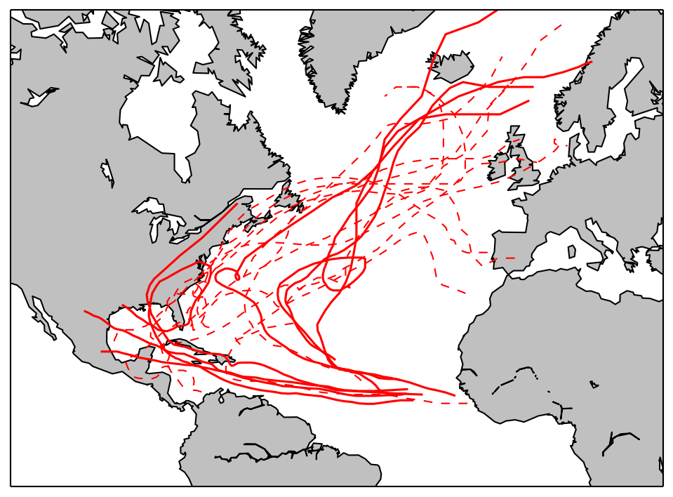
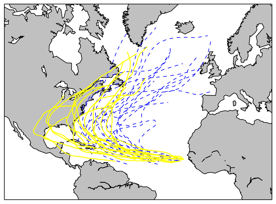
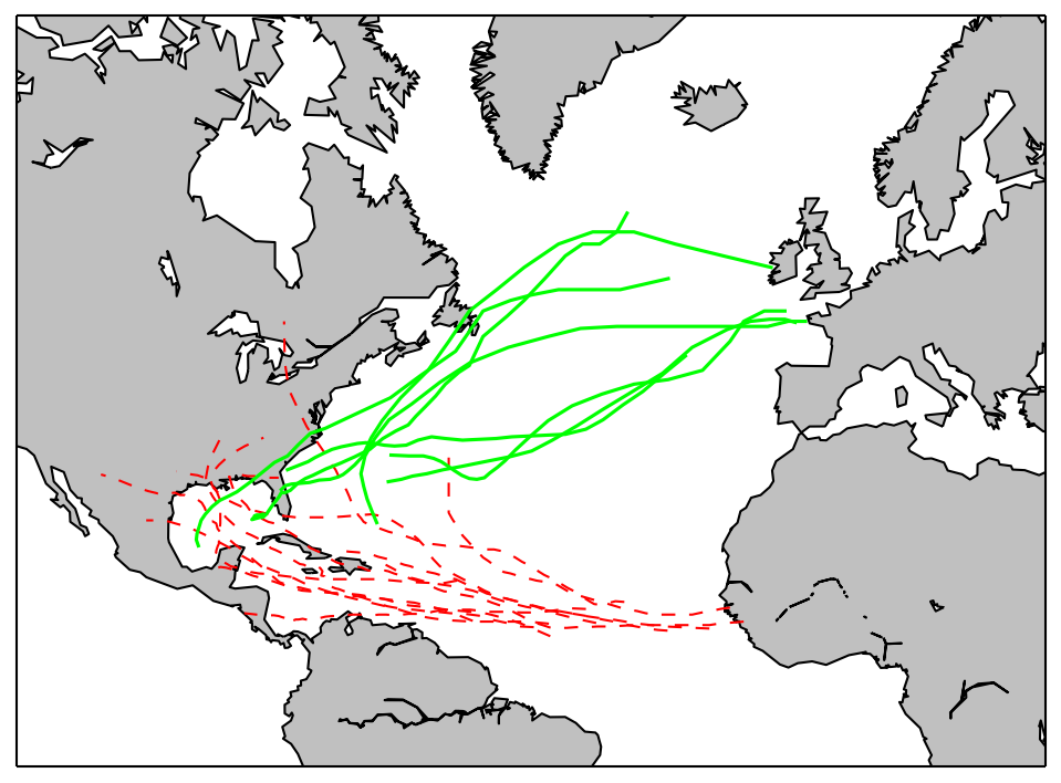
We use hurricane data from 1970 to 2010 provided by the National Oceanic and Atmospheric Administration (NOAA) in this experiment. The data provides a time series of longitude and latitude coordinates for each storm, effectively forming a GPS trace. In order to compare the overall shape of these traces we use the discrete Fréchet distance (Eiter and Mannila, 1994). Intuitively this measures the minimal distance required to connect points on two curves being compared, i.e. structurally similar curves have a low score. Before computing the Fréchet distance between two curves we move their starting points to the same location. This means that we are comparing their shapes and not their global location. Clustering the $700$ traces using the LD method with $\ell=20$ we obtain clusters that move in a similar direction, as shown in hurricanes_1970 b) and c). Analysing the outliers shown in hurricanes_1970 a) we find that half of them are category 4 and 5 Cape Verde-type hurricanes, shown by the thick stroke. The other half of the outliers were selected due to either their long life time, unusual motion, or high destructive power and are shown with dashed stroke. This demonstrates that the outliers found by the proposed methods find interesting patterns in spatial temporal data which are not directly apparent.

(a) Exemplars

(b) Outliers

Figure 8: Evolution of the $\lambda$ values of select exemplars and outliers over the iterations. In both cases we can observe how after about 150 iterations the values have stabilised. Additionally, outliers have higher $\lambda$ values and exhibit less variation compared to exemplars.

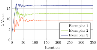
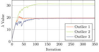
To better understand the behaviour of LD we plot the value of the $\lambda$ values associated with representative outliers and exemplars in ld-evolution. One can see how after about 100 iterations the values level out and remain stable. Interestingly the outliers have higher $\lambda$ values compared to the exemplars which allows the method to distinguish between them more easily. Lastly, the outliers have smoother curves, i.e. less jumps, when compared to the exemplars. This indicates that outliers do not change significantly whereas exemplars will change during the optimisation process. Overall, stable results are achieved after about a third of the runtime suggesting that a more sophisticated termination criterion can be used for faster convergence.

4.3 MNIST Data

(a) Digit 1

(b) Digit 4

(c) Outliers

Figure 9: Each row in (a) and (b) shows a different appearance of a digit captured by a cluster. The outliers shown in (c) tend to have heavier then usual stroke, are incomplete or are not recognisable as a digit.

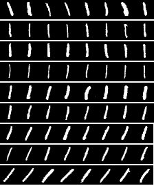
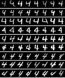
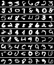
The MNIST dataset, introduced by LeCun et al. (1998), contains $28\times 28$ pixel images of handwritten digits. We extract features from these images by representing them as 768 dimensional vectors which is reduced to 25 dimensions using PCA. $L2$ norm is used to compute the distance between these vectors. In mnist we show exemplary results obtained when processing $10\,000$ digits with the LD method with $\theta=5$ and $\ell=500$. Each row in mnist a) and b) shows examples of clusters representing the digits 1 and 4 respectively. This illustrates how different the same digit can appear and the separation induced by the clusters. mnist c) contains a subset of the outliers selected by the method. These outliers have different characteristics that make them sensible outliers, such as: thick stroke, incomplete, unrecognisable or ambiguous meaning.

To investigate the influence the cluster creation cost has we run the experiment with different values of $\theta$. In mnist-evaluation we show results for values of cost scaling factor $\theta=\{5,15,25\}$. The V-Measure score does not change drastically between the different runs. However, the other measures, especially the number of clusters changes. We can see that, as expected, by increasing the cost the number of clusters decreases. This results in an increased completeness score, i.e. a larger percentage of the same ground truth labels are contained in a smaller number of clusters. Meanwhile, the homogeneity score drops which indicates that there are more cases of different digits that look similar, such as $1$ and $7$, being placed into a single cluster. Overall, we can say that changes to the cluster creation cost has a predictable impact on the results with no apparent sudden changes.

Table 2: Evaluation of clustering results of the MNIST data set with different cost scaling values $\theta$. We can see that increasing the cost results in fewer clusters but as a trade off reduces the homogeneity of the clusters.

$\theta$	$5$	$15$	$25$
V-Measure	$0.51$	$0.53$	$0.53$
Homogeneity	$0.82$	$0.73$	$0.70$
Completeness	$0.37$	$0.42$	$0.43$
Clusters	$82$	$36$	$21$

4.4 Natural Scenes Data

Figure 10: Results obtained when clustering the image dataset using APOC. The rows contain, car outliers, cup outliers, cluster 1, cluster 2 and cluster 3 respectively. The three clusters differ in their colour scheme: the first one has muted tones, the second is dominated by cold white and blue tones, while the third one contains vibrant colours.

Table 3: Energy relative to the LP solution obtained on the natural scenes data set. APOC and LD obtain energy values which are nearly identical to LP and find all the correct outliers. k-means– only finds suboptimal solutions and thus struggles to find good outliers unless the correct value for $k$ is specified.

Method	Energy	Clusters	Jaccard Index
LP	$100.0\%$	$3$	$1$
APOC	$96.6\%$	$3$	$1$
LD	$95.3\%$	$3$	$1$
k-means–	$81.3\%$	$1$	$0.54$
k-means–	$85.2\%$	$3$	$0.93$
k-means–	$83.8\%$	$5$	$0.64$

In this section we apply APOC to outlier detection in image collections. Our dataset is composed of images from mountain ranges with outliers in the form of cars and coffee cups. The distance between images is computed from colour histograms and local binary pattern (Ojala et al., 2002) histograms using the Bhattacharyya distance. When we specify the correct number of outliers APOC and LD find all of the images belonging to our two outlier groups and cluster the remaining images according to their appearance. image-data-results shows outliers in the first two rows and examples belonging to the three clusters found in subsequent rows as found by APOC. The three clusters contain images which mainly differ in their colour and mood. The first cluster contains images with muted greens and browns, the second cluster has images with cold white and blue colours and finally the last cluster is dominated by vibrant colours. For comparison we also process this data using LP, LD and k-means–. The results in lp-comparison show how close the different methods come to the optimal energy, the number of clusters and the quality of the selected outliers. This shows that APOC and LD perform nearly as well as the optimal LP solution, while k-means– depends on a good choice of $k$ and still fails to recover all the outliers. This experiment also highlights the capability of APOC and LD to pick communities of points as outliers in a global scope.

5 Related work

In introduction, we provided some context for combining clustering and outlier detection. Here we elaborate further on other works which are germane to our problem. The problem of outlier detection has been extensively researched in both statistics and data mining (Chandola et al., 2009; Hawkins, 1980). However, both communities have different perspectives. The statistical perspective is to design models which are robust against outliers. In the process, outliers are discovered and evaluated. The data mining perspective is to directly mine for outliers and then determine their usefulness. The study of outlier detection in data mining was pioneered by the work of Knorr and Ng (1997) who proposed a definition of distance-based outliers which relaxed strict distributional assumptions and was readily generalisable to multi-dimensional data sets. Following Knorr and Ng, several variations and algorithms have been proposed to detect distance-based outliers (Bay and Schwabacher, 2003; Ramaswamy et al., 2000). However, the outliers detected by these methods are global outliers, i.e., the “outlierness” is with respect to the whole dataset. Breunig et al. (2000) have argued that in some situations local outliers are more important than global outliers and cannot be easily detected by standard distance-based techniques. They introduced the concept of local outlier factor ($LOF$), which captures how isolated an object is with respect to its surrounding neighbourhood. The concept of local outliers has subsequently been extended in several directions (Chandola et al., 2009; Chawla and Sun, 2006; Papadimitriou et al., 2003).

Despite the observation that clustering and outlier detection techniques should naturally complement each other, research work in integrating the two is limited. The MCD (as noted in the Introduction), is one prominent approach where the problem of outliers was tightly integrated in an optimisation framework (Rousseeuw and Driessen, 1999). The k-means– approach extended the idea of MCD to include clustering (Chawla and Gionis, 2013). The theoretical research in combining clustering and outlier detection has been investigated in the context of robust versions of the k-median and facility location problems (Chen, 2008; Charikar et al., 2001). However, as noted before, the focus has exclusively been on deriving theoretical approximation bounds. To the best of our knowledge the use of belief propagation ideas to investigate outliers is entirely novel.

6 Conclusion

In this paper we presented a novel approach to joint clustering and outlier detection formulated as an integer program. The proposed optimisation problem enforces valid clusters as well as the selection of a fixed number of outliers. We then described three ways of solving the optimisation problem using (i) linear programming, (ii) affinity propagation with outlier detection and (iii) Lagrangian duality. Experiments on synthetic and real data show how the joint optimisation outperforms two stage approaches such as k-means–. Additionally, experimental results suggest that results obtained via APOC and LD are very close to the optimal solution at a fraction of the computational time. Finally, we detail the modifications of the LD method, needed to process large scale datasets.

References

- Arthur and Vassilvitskii [2007] D. Arthur and S. Vassilvitskii. k-means++: The Advantages of Careful Seeding. In ACM-SIAM Symposium on Discrete Algorithms, 2007.
- Bay and Schwabacher [2003] S. Bay and M. Schwabacher. Mining distance-based outliers in near linear time with randomization and a simple pruning rule. In Int. Conf. on Knowledge Discovery and Data Mining, 2003.
- Bertsimas and Weismantel [2005] D. Bertsimas and R. Weismantel. Optimization over Integers. Dynamic Ideas Belmont, 2005.
- Breunig et al. [2000] M. Breunig, H. Kriegel, R. Ng, and J. Sander. LOF: Identifying Density-Based Local Outliers. In Int. Conf. on Management of Data, 2000.
- Chandola et al. [2009] V. Chandola, A. Banerjee, and V. Kumar. Anomaly detection: A survey. ACM Computing Surveys, 2009.
- Charikar et al. [2001] M. Charikar, S. Khuller, D. M. Mount, and G. Narasimhan. Algorithms for Facility Location Problems with Outliers. In Proc. of the ACM-SIAM Symposium on Discrete Algorithms, 2001.
- Chawla and Gionis [2013] S. Chawla and A. Gionis. k-means–: A Unified Approach to Clustering and Outlier Detection. In SIAM International Conference on Data Mining, 2013.
- Chawla and Sun [2006] S. Chawla and P. Sun. SLOM: A new measure for local spatial outliers. Knowledge and Information Systems, 2006.
- Chen [2008] K. Chen. A constant factor approximation algorithm for -median clustering with outliers. In Proc. of the ACM-SIAM Symposium on Discrete Algorithms, 2008.
- Croux and Ruiz-Gazen [1996] C. Croux and A. Ruiz-Gazen. A Fast Algorithm for Robust Principal Components Based on Projection Pursuit. In Proc. in Computational Statistics, 1996.
- Cuesta-Albertos et al. [1997] J. Cuesta-Albertos, A. Gordaliza, and C. Matrán. Trimmed -means: an attempt to robustify quantizers. The Annals of Statistics, 1997.
- Eiter and Mannila [1994] T. Eiter and H. Mannila. Computing Discrete Fréchet Distance. Technical report, Technische Universität Wien, 1994.
- Frey and Dueck [2007] B. Frey and D. Dueck. Clustering by Passing Messages Between Data Points. Science, 2007.
- Garc a-Escudero et al. [2010] L. Garc a-Escudero, A. Gordaliza, C. Matr n, and A. Mayo-Iscar. A Review of Robust Clustering Methods. Advances in Data Analysis Classification, 2010.
- Givoni and Frey [2009] I. Givoni and B. Frey. A Binary Variable Model for Affinity Propagation. Neural Computation, 2009.
- Hawkins [1980] D. Hawkins. Identification of Outliers. Chapman and Hall, London, 1980.
- Hennig [2008] C. Hennig. Dissolution point and isolation robustness: Robustness criteria for general cluster analysis methods. Journal of Multivariate Analysis, 2008.
- Huber and Ronchetti [2008] P. Huber and E. Ronchetti. Robust Statistics. Wiley, 2008.
- Knorr and Ng [1997] E. Knorr and R. Ng. A Unified Notion of Outliers: Properties and Computation. In Int. Conf. on Knowledge Discovery and Data Mining, 1997.
- Komodakis et al. [2008] N. Komodakis, N. Paragios, and G. Tziritas. Clustering via LP-based Stabilities. In Advances in Neural Information Processing Systems, 2008.
- Kschischang et al. [2001] F. R. Kschischang, B. J. Frey, and H.-A. Loeliger. Factor Graphs and the Sum-Product Algorithm. IEEE Transactions on Information Theory, 2001.
- LeCun et al. [1998] Y. LeCun, L. Bottou, Y. Bengio, and P. Haffner. Gradient-based learning applied to document recognition. Proceedings of the IEEE, 1998.
- Ojala et al. [2002] T. Ojala, M. Pietikainen, and T. Maenpaa. Multiresolution Gray-Scale and Rotation Invariant Texture Classification with Local Binary Patterns. IEEE Transactions on Pattern Analysis and Machine Intelligence, 2002.
- Papadimitriou et al. [2003] S. Papadimitriou, H. Kitagawa, P. Gibbons, and C. Faloutsos. LOCI: Fast outlier detection using the local correlation integral. In Int. Conf. on Data Engineering, 2003.
- Ramaswamy et al. [2000] S. Ramaswamy, R. Rastogi, and K. Shim. Efficient Algorithms for Mining Outliers from Large Data Sets. In Int. Conf. on Management of Data, 2000.
- Rosenberg and Hirschberg [2007] A. Rosenberg and J. Hirschberg. V-Measure: A conditional entropy-based external cluster evaluation measure. In Proc. of the Joint Conference on Empirical Methods in Natural Language Processing and Computational Natural Language Learning, 2007.
- Rousseeuw and Driessen [1999] P. Rousseeuw and K. Driessen. A fast algorithm for the minimum covariance determinant estimator. Technometrics, 1999.
- Weiss et al. [2007] Y. Weiss, C. Yanover, and T. Meltzer. MAP Estimation, Linear Programming and Belief Propagation with Convex Free Energies. In Proc. of the Conference on Uncertainty in Artificial Intelligence, 2007.
- Wright et al. [2009] J. Wright, A. Ganesh, S. Rao, Y. Peng, and Y. Ma. Robust Principal Component Analysis: Exact Recovery of Corrupted Low-Rank Matrices by Convex Optimization. In Advances in Neural Information Processing Systems, 2009.