Dynamic sampling schemes for optimal noise learning
under multiple nonsmooth constraints

Abstract

We consider the bilevel optimisation approach proposed in [5] for learning the optimal parameters in a Total Variation (TV) denoising model featuring for multiple noise distributions. In applications, the use of databases (dictionaries) allows an accurate estimation of the parameters, but reflects in high computational costs due to the size of the databases and to the nonsmooth nature of the PDE constraints. To overcome this computational barrier we propose an optimisation algorithm that, by sampling dynamically from the set of constraints and using a quasi-Newton method, solves the problem accurately and in an efficient way.

1 Introduction

Most images in the real world suffer from noise. In photography noisy images occur when taking a photograph under bad lighting conditions, for instance. Medical imaging applications, such as Magnetic Resonance Imaging (MRI) and Positron Electron Tomography (PET), produce under-sampled and noisy image data. In general, the quality of images obtained from imaging devices in the real world, in the sciences and medicine, is limited by the hardware and the limited time available to measure the image data. Hence, one of the most important tasks in image processing is the reduction of noise in images, called image denoising.

A common challenge in image denoising is the setup of a suitable denoising model. The model depends on the noise distribution and the class of images the denoised solution should belong to. In [5] a bilevel optimisation approach to learn the correct setup for a TV denoising model from a set of noisy and clean test images is proposed. There, optimal parameters $\lambda_{i}\in\mathbb{R},i=1,\ldots,d$ are determined by solving the following optimisation problem:

$$\min_{\lambda_{i}\geq 0,\ i=1,\ldots,d}\,\frac{1}{2N}\sum_{k=1}^{N}\left\lVert\hat{u}_{k}-u_{k}\right\rVert^{2}_{L^{2}(\Omega)}$$ (1.1)

subject to the set of nonsmooth constraints:

$$\hat{u}_{k}=\text{argmin}_{u\in BV(\Omega)\cap\mathcal{A}}\left(|Du|(\Omega)+\sum_{i=1}^{d}\lambda_{i}\int_{\Omega}\phi_{i}(u,f_{k})\,dx\right),\quad k=1,\ldots,N.$$ (1.2)

In (1.1)-(1.2) $\Omega\subset\mathbb{R}^{2}$ is the image domain, $|Du|(\Omega)$ is the Total Variation (TV) $u$ in $\Omega$ and $BV(\Omega)$ is the space of functions of bounded variation (see [1]). For each $k$, the pair $(u_{k},f_{k})$ is an element of a set of $N$ pairs of clean and noisy test images, respectively, whereas $\hat{u}_{k}$ is the TV-denoised version of $f_{k}$. For $i=1,\ldots,d\$ the terms $\phi_{i}$ represent the different data fidelities, each one modelling one particular type of noise weighted by a parameter $\lambda_{i}$. Examples of $\phi$ are $\phi(u,f_{k})=(u-f_{k})^{2}$ for noise with Gaussian distribution and $\phi(u,f_{k})=|u-f_{k}|$ for the case of impulse noise. The set $\mathcal{A}$ is the set of admissible functions such that the data fidelity terms are well defined.

In this paper, we use a simulated database of clean and noisy images. This is not uncommon. Even in real world applications such as MRI, simulated databases are used to tune image retrieval systems, see for instance [7]. Alternatively, we can imagine the retrieval of such a test set for a specific application using phantoms and their noisy acquisitions. Ideally, we would like to consider a very rich database (i.e. $N\gg 1$) in order to get a more robust estimation of the parameters, thus dealing with a very large set of constraints (1.2) that would need to be solved in each iteration of an optimisation algorithm applied to (1.1)-(1.2). The computational solution of such an optimisation problem renders expensive and therefore challenging due to the large-scale nature of the problem (1.1)-(1.2) and due to the nonsmooth nature of each constraint.

In order to deal with such large-scale problems various stochastic optimisation approaches have been presented in literature. They are based on the common idea of solving not all the PDE constraints, but just a sample of them, whose size varies according to the approach one intends to use. In this paper we focus on a stochastic approximation method proposed by Byrd et al. [3] called dynamic sample size method. The main idea of this method is to consider an initial, small, training sample of the dictionary to start the algorithm with and dynamically increasing its size, if needed, throughout the different steps of the optimisation process. The criterion to decide whether or not the sample size has to be increased is a check on the sample variance estimates on the batch gradient. The desired trade-off between efficiency and accuracy is then obtained by starting with a small sample and gradually increasing its size till reaching the requested level of accuracy. Let us mention that the method of Byrd et al. is one among various stochastic optimisation methods, compare for instance [8, 10, 2, 6, 9].

Our work extends the work of [3] in two directions: firstly, in [3] the linearity of the solution map is required which is not fulfilled for our problem (1.1)-(1.2). We are going to show that the strategy of Byrd et al. can be modified for nonlinear solution maps as the one we are considering. Secondly, in [3] the optimization algorithm is of gradient-descent type. Using a BFGS method to solve (1.1)-(1.2) we extend their approach incorporating also second order information in form of an approximation of the Hessian by evaluations of the sample gradient in the iterations of the optimisation algorithm.

Organisation of the paper. In the following Section 2 we present the Dynamic Sampling algorithm adapted to the nonlinear framework of problem (1.1)-(1.2), specifying the variance condition on the batch gradient used in our optimisation algorithm. In Section 3 we present the numerical results obtained for the estimation of the optimal parameters in the case of single and mixed noise estimation for the model (1.1)-(1.2) showing significant improvements in efficiency.

Preliminaries. We denote the vector of parameters we aim to estimate by $\bm{\lambda}=(\lambda_{1},\ldots,\lambda_{d})\in\mathbb{R}^{d}_{\geq 0}$. We also define by $\mathcal{S}$ the solution map that, for each constraint $k=1,\ldots,N$ of (1.2), associates to $\bm{\lambda}$ and to the noisy image $f_{k}$ the corresponding Total Variation denoised solution $\hat{u}_{k}$, that is $\mathcal{S}(\bm{\lambda},f_{k})=\hat{u}_{k}$. Let us then define the reduced cost functional $J(\bm{\lambda})$ as

$$J(\bm{\lambda}):=\frac{1}{2N}\sum_{k=1}^{N}\left\lVert\mathcal{S}(\bm{\lambda},f_{k})-u_{k}\right\rVert^{2}_{L^{2}(\Omega)}$$ (1.3)

We also define:

$$l(\bm{\lambda},f_{k}):=\left\lVert\mathcal{S}(\bm{\lambda},f_{k})-u_{k}\right\rVert^{2}_{L^{2}(\Omega)},\quad k=1,\dots,N$$ (1.4)

as the loss functions of the functional $J$ defined in (1.3) for each $k=1,\ldots,N$. For every sample $S\subset\left\{1,\ldots,N\right\}$ of the database, we introduce the batch objective function:

$$J_{S}(\bm{\lambda}):=\frac{1}{2|S|}\sum_{k\in S}l(\bm{\lambda},f_{k})$$ (1.5)

2 Dynamic sampling schemes for solving (1.1)-(1.2)

To design the optimisation algorithm solving (1.1)-(1.2) we follow the approach used in [5]. There, a quasi-Newton method (namely, the Broyden-Fletcher -Goldfarb-Shanno algorithm BFGS) is considered together with an Armijo backtracking linesearch rule. We combine such algorithm with a modified version of the Dynamic Sampling algorithm presented in [3, Section 3]. In order to compare our algorithm with the Newton-Conjugate Gradient method presented in [3, Section 5], we highlight that in our optimisation algorithm the Hessian matrix is never computed, but approximated efficiently by the BFGS matrix.

Our algorithm starts by selecting from the whole dataset a sample $S$ whose size $|S|$ is small compared to the original size $N$. In the following iterations, if the approximation computed produces an improvement in the cost functional $J$, then the sample size is kept unchanged and the optimisation process continues selecting in the next iteration a new sample of the same size. Otherwise, if the approximation computed is not a good one, a new, larger, sample size is selected and a new sample $S$ of this new size is used to compute the new step. By starting with small sample sizes it is hoped that in the early stages of the algorithm the solution can be computed efficiently in each iteration. The key point in this procedure is clearly the rule that checks throughout the progression of the algorithm, whether the approximation we are performing is good enough, i.e. the sample size is big enough, or has to be increased. Because of this systematic check on the quality of approximation in each step of the algorithm, such sampling strategy is called dynamic.

As in [3], we consider a condition on the batch gradient $\nabla J_{S}$ which imposes in every stage of the optimisation that the direction $-\nabla J_{S}$ is a descent direction for $J$ at $\bm{\lambda}$ if the following condition holds:

$$\left\lVert\nabla J_{S}(\bm{\lambda})-\nabla J(\bm{\lambda})\right\rVert_{L^{2}(\Omega)}\leq\theta\left\lVert\nabla J_{S}(\bm{\lambda})\right\rVert_{L^{2}(\Omega)},\quad\theta\in[0,1).$$ (2.6)

The computation of $\nabla J$ may be very expensive for applications involving large databases and nonlinear constraints, so we rewrite (2.6) as an estimate of the variance of the random vector $\nabla J_{S}(\bm{\lambda})$. In order to do that, recalling definitions (1.4) and (1.5) we observe that

$$\nabla J_{S}(\bm{\lambda})=\frac{1}{2|S|}\sum_{k\in S}\nabla l(\bm{\lambda},f_{k})$$ (2.7)

We can compute (2.7) in correspondence to an optimal solution $\bm{\hat{\lambda}}$ by using [5, Remark 3.4] where a characterisation of $\nabla J$ is given in terms of the adjoint states $p_{k}$ (see Section 3 for details). By linearity and extending to the multiple-constrained case, we get:

$$\nabla J_{S}(\bm{\hat{\lambda}})=\sum_{k\in S}\sum_{i=1}^{d}\int_{\Omega}\phi_{i}^{\prime}(\hat{u}_{k},f_{k})\,p_{k}\,dx$$ (2.8)

Thanks to this characterisation, we now extend the dynamic sampling algorithm in [3] to the case where the solution map $\mathcal{S}$ is nonlinear: by taking (2.8) into account and following [3, Section 3] we can rewrite (2.6) as a condition on the variance of the batch gradient that reads as

$$\frac{\left\lVert Var_{k\in S}(\nabla l(\bm{\lambda},f_{k}))\right\rVert_{L^{1}(\Omega)}}{|S|}\frac{N-|S|}{N-1}\leq\theta^{2}\left\lVert\nabla J_{S}(\bm{\lambda})\right\rVert^{2}_{L^{2}(\Omega)}.$$ (2.9)

For a detailed derivation of (2.9), see [3]. Condition (2.9) is the responsible for possible changes in the sample size in the optimisation algorithm and has to be checked in every iteration. If inequality (2.9) is not satisfied, a larger sample $\hat{S}$ whose size satisfies the descent condition (2.9) needs to be considered. By assuming that the change in the sample size is gradual enough such that, for any given $\bm{\lambda}$:

$$\left\lVert Var_{k\in\hat{S}}(\nabla l(\bm{\lambda},f_{k}))\right\rVert_{L^{1}(\Omega)}\approx\left\lVert Var_{k\in S}(\nabla l(\bm{\lambda},f_{k}))\right\rVert_{L^{1}(\Omega)},$$

$$\left\lVert\nabla J_{\hat{S}}(\bm{\lambda})\right\rVert_{L^{2}(\Omega)}\approx\left\lVert\nabla J_{S}(\bm{\lambda})\right\rVert_{L^{2}(\Omega)},$$

we see that condition (2.9) is satisfied whenever we choose $|\hat{S}|$ such that

$$|\hat{S}|\geq\Bigg{\lceil}\frac{N-\left\lVert Var_{k\in S}(\nabla l(\bm{\lambda},f_{k}))\right\rVert_{L^{1}(\Omega)}}{\left\lVert Var_{k\in S}(\nabla l(\bm{\lambda},f_{k}))\right\rVert_{L^{1}(\Omega)}+\theta^{2}(N-1)\left\lVert\nabla J_{S}(\bm{\lambda})\right\rVert^{2}_{L^{2}(\Omega)}}\Bigg{\rceil}.$$ (2.10)

Conditions (2.9) and (2.10) are the key points in the optimisation algorithm we are going to present: by checking the former, one can control whether the sampling approximation is accurate enough and if this is not the case at any stage of the algorithm, by imposing the latter a new larger sample size is determined.

We remark that these two conditions force the direction $-\nabla J_{S}$ to be a descent direction. Steepest descent methods are known to be slowly convergent. Algorithms incorporating information coming from the Hessian are generally more efficient. However, normally the computation of the Hessian is very expensive, so Hessian-approximating methods are commonly used. In [3] a Newton-CG method is employed. There, an approximation of the Hessian matrix $\nabla^{2}J_{S}$ is computed only on a subsample $H$ of $S$ such that $|H|\ll|S|$. As the sample $S$ is dynamically changing, the subsample $H$ will change as well (with a fixed, constant ratio) and the computation of the new conjugate gradient direction can be performed efficiently. In this work, in order to compute an approximation of the Hessian we consider the well-known BFGS method which has been extensively used in the last years because of its efficiency and low computational costs.

Before giving a full description of the resulting algorithm solving (1.1)-(1.2), we briefly comment on the linesearch rule that is employed in the update of the BFGS matrix. We choose an Armijo backtracking line search rule with curvature verification: the BFGS matrix is updated only if the curvature condition is satisfied. The Amijo criterion is:

$$J_{S}(\bm{\lambda_{k}}+\alpha_{k}d_{k})-J_{S}(\bm{\lambda_{k}})\leq\alpha_{k}\eta\nabla J_{S}(\bm{\lambda_{k}})^{\top}d_{k}$$ (2.11)

where the value $\eta$ will be specified in Section 3, $d_{k}$ is the descent direction of the quasi-Newton step, $\alpha_{k}$ is the length of the quasi-Newton step and $\nabla J_{S}(\bm{\lambda_{k}})$ is defined in (2.7) . The positivity of the parameters is always preserved along the iterations.

We present now the BFGS optimisation with Dynamic sampling for solving (1.1)-(1.2): compared to [3, Algorithm 5.2] we stress once more that the gain in efficiency is obtained thanks to the use of BFGS instead of the Newton-CG sampling method.

Algorithm 1 Dynamic Sampling BFGS for solving (1.1)-(1.2)

1:  Initialize: $\bm{\lambda_{0}}$, sample $\mathcal{S}_{0}$ with $|S_{0}|\ll N$ and model parameter $\theta$, $k=0$.

2:  while BFGS not converging, $k\geq 0$

3:   sample $|S_{k}|$ PDE constraints to solve;

4:   update of the BFGS matrix;

5:   compute direction $d_{k}$ by BFGS and steplength $\alpha_{k}$ by Armijo cond. (2.11);

6:   define new iterate: $\bm{\lambda_{k+1}}=\bm{\lambda_{k}}+\alpha_{k}d_{k}$;

7:   if condition (2.9) then

8:    maintain the sample size: $|S_{k+1}|=|S_{k}|$;

9:   else augment $S_{k}$ such that condition (2.10) is verified.

10:  end

3 Numerical results

In this section we present the numerical results of the Dynamic Sampling Algorithm 1 applied to compute the numerical solution of (1.1)-(1.2). In our numerical computations we fix the parameter values as follows:

• We consider images of size $150\times 150$. We approximate the differential operators by discretising with finite difference schemes with mesh step size $h=1/$(number of pixels in the $x$-direction). We use forward difference for the discretisation of the divergence operator and backward differences for the gradient. The Laplace operator is discretised by using the usual five point formula.

• The TV constraints in (1.2) are solved by means of SemiSmooth Newton (SSN) algorithms whose form depends on the $\phi$’s in (1.2) (cf. [5, Section 4]) solving regularised problems which stop if either the difference between two consecutive iterates is small enough or if the maximum number of iterations $\textsf{maxiter}=35$ is reached.

• In the Armijo condition (2.11) the value $\eta$ is chosen to be $\gamma=10^{-4}$.

Single noise estimation.

As a toy example, we start by considering the case when the noise in the images is normally distributed. In (1.1)-(1.2), this reflects in the estimation of just one parameter $\lambda$ that weights the fidelity term $\phi(u,f_{k})=(u-f_{k})^{2}$ in each constraint. Considering the training database $\left\{(u_{k},f_{k})\right\}_{k=1,\ldots,N}$ of clean and noisy images, the problem reduces to:

$$\min_{\lambda\geq 0}\,\frac{1}{2N}\sum_{k=1}^{N}\left\lVert\hat{u}_{k}-u_{k}\right\rVert^{2}_{L^{2}(\Omega)}$$ (3.1)

where, for each $k$, $\hat{u}_{k}$ is the solution of the regularised PDE

$$-\varepsilon\Delta\hat{u}_{k}-\text{div}\Big{(}h_{\gamma}(\nabla\hat{u}_{k})\Big{)}+\lambda(\hat{u}_{k}-f_{k})=0,\quad k=1,\dots,N.$$ (3.2)

In (3.2) $h_{\gamma}$ arises from a Huber-type regularisation of the subdifferential of $|D\hat{u}_{k}|$ with parameter $\gamma\gg 1$ and the $\varepsilon$ term is an artificial diffusion term that sets up the problem in the Hilbert space $H^{1}_{0}(\Omega)$ (see [5, Section 3] for details).

As shown in [5, Theorem 3.5] the adjoint states $p_{k}$ can be computed for each constraint as the solution of the following equation

$$\varepsilon(Dp_{k},Dv)_{L^{2}}+(h_{\gamma}^{\prime}(D\hat{u}_{k})^{*}Dp_{k},Dv)_{L^{2}}\\ +\int_{\Omega}\lambda\leavevmode\nobreak\ p_{k}\leavevmode\nobreak\ v\leavevmode\nobreak\ dx=-(\hat{u}_{k}-f_{k},v)_{L^{2}},\quad\forall v\in H_{0}^{1}(\Omega).$$ (3.3)

Recalling also equations (2.7)-(2.8) needed for the computation of the gradient, we can now apply Algorithm 1 to solve (3.1)-(3.2).

For the following numerical tests, the parameters of this model are chosen as follows: $\varepsilon=10^{-12},\gamma=100$. The noise in the images has distribution $\mathcal{N}(0,0.05)$. The parameter $\theta$ of the Algorithm 1, is chosen to be $\theta=0.5$. We will comment on the sensitivity of the method to $\theta$ later on.

Table 1 shows the numerical value of the optimal parameter $\hat{\lambda}$ when varying the size of the dictionary. We measure the efficiency of the algorithms used in terms of the number of nonlinear PDEs solved during the BFGS optimisation and we compare the efficiency of solving (3.1)-(3.2) without and with the Dynamic Sampling strategy. We observe a clear improvement in efficiency when using Dynamic Sampling: the number of PDEs solved in the optimisation process is very much reduced. We note that this corresponds to an increasing number of BFGS iterations which does not appear to be an issue as BFGS iterations are themselves very fast. For the sake of computational efficiency, what really matters is the number of PDEs that need to be solved in each iteration of BFGS. Moreover, thanks to modern parallel computing methods and to the decoupled nature of the constraints in each BFGS iteration, solving such a reduced amount of PDEs makes the computational efforts very reasonable. In fact, we note that the size of the sample is generally maintained very small in comparison to $N$ or just slightly increased. Computing also the relative error between the optimal parameter computed by solving all the PDEs and the one computed with Dynamic Sampling method, we note a good level of accuracy: the difference between the two values remains below $5\%$.

$N$	$\hat{\lambda}$	$\hat{\lambda}_{S}$	$|S_{0}|$	$|S_{end}|$	eff.	eff. Dyn.S.	BFGS its.	BFGS its. Dyn.S.	diff.
$10$	$3334.5$	$3427.7$	$2$	$3$	$140$	$84$	$7$	$21$	$2.7\%$
$20$	$3437.0$	$3475.1$	$4$	$4$	$240$	$120$	$7$	$15$	$1.1\%$
$30$	$3436.5$	$3478.2$	$6$	$6$	$420$	$180$	$7$	$15$	$1.2\%$
$40$	$3431.5$	$3358.3$	$8$	$9$	$560$	$272$	$7$	$16$	$2.1\%$
$50$	$3425.8$	$3306.4$	$10$	$10$	$700$	$220$	$7$	$11$	$3.5\%$
$60$	$3426.0$	$3543.4$	$12$	$12$	$840$	$264$	$7$	$11$	$3.3\%$
$70$	$3419.7$	$3457.7$	$14$	$14$	$980$	$336$	$7$	$12$	$1.1\%$
$80$	$3418.1$	$3379.3$	$16$	$16$	$1120$	$480$	$7$	$15$	$<1\%$
$90$	$3416.6$	$3353.5$	$18$	$18$	$1260$	$648$	$7$	$18$	$2.3\%$
$100$	$3413.6$	$3479.0$	$20$	$20$	$1400$	$520$	$7$	$13$	$1.9\%$

Table 1: $N$ is the size of the database, $\hat{\lambda}$ is the optimal parameter for (3.1)-(3.2) obtained by solving all the $N$ constraints, whereas $\hat{\lambda}_{S}$ is the one computed by solving the problem with Algorithm 1. The initial size $S_{0}$ is chosen to be $|S_{0}|=20\%N$. $|S_{end}|$ of the sample at the end of the optimisation algorithm. The efficiency of the algorithms is measured in terms of the PDEs solved. We compare the accuracy of the approximation in terms of the difference $\left\lVert\hat{\lambda}_{S}-\hat{\lambda}\right\rVert_{1}/\left\lVert\lambda_{S}|\right\rVert_{1}$.

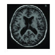
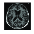
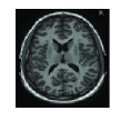
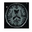
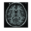
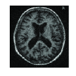
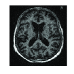
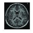
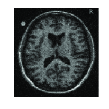
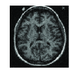
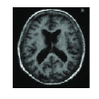
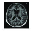
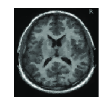
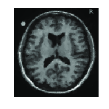
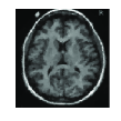
Figure 1 shows an example of database of brain images together with the optimal denoised version obtained by Algorithm 1 for single Gaussian noise estimation.

Figure 1: Sample of $5$ images of a MRI brain database: original images (upper row), noisy images (middle row) and optimal denoised images (bottom row), $\hat{\lambda_{S}}=3280.5$.

Multiple noise estimation.

We consider now a more interesting application of (1.1)-(1.2) where the image is corrupted by noises with different distributions. We consider the case where a combination of Gaussian and impulse noise is present. The fidelity term for the impulse distributed component is $\phi_{1}(u,f_{k})=|u-f_{k}|$, whereas, as above, for the Gaussian noise we consider the fidelity $\phi_{2}(u,f_{k})=(u-f_{k})^{2}$, for every $k$. Each fidelity term is weighted by a parameter $\lambda_{i},i=1,2$. Thus, we aim to solve:

$$\min_{(\lambda_{1},\lambda_{2}),\ \lambda_{i}\geq 0}\,\frac{1}{2N}\sum_{k=1}^{N}\left\lVert\hat{u}_{k}-u_{k}\right\rVert^{2}_{L^{2}(\Omega)}$$ (3.4)

where, for each $k$, $\hat{u}_{k}$ is now the solution of the regularised PDE:

$$-\varepsilon\Delta\hat{u}_{k}-\text{div}(h_{\gamma}(\nabla\hat{u}_{k}))+\lambda_{1}h^{1}_{\gamma}(\hat{u}_{k}-f_{k})+\lambda_{2}(\hat{u}_{k}-f_{k})=0,\quad k=1,\ldots,N.$$ (3.5)

In (3.5) the first and the second terms are as before while the third one corresponds to the Huber-type regularisation of $\text{sgn}(\hat{u}_{k}-f_{k})$. The adjoint state is computed as in [5], in a similar manner as (3.3). By taking also into account equations (2.7)-(2.8), we solve (3.4)-(3.5) with $\varepsilon=10^{-12},\gamma=100$ by means of Algorithm 1.

We take as example slices of the brain database shown in Figure 1 corrupted with both Gaussian noise distributed as $\mathcal{N}(0,0.005)$ and impulse noise with fraction of missing pixels $d=5\%$, and again solve (1.1)-(1.2) by solving the PDE constraints all at once and by using Dynamic Sampling for different $N$. In Table 2 we report the results for the estimation of $\lambda_{1}$ and $\lambda_{2}$.

$N$	$\hat{\lambda_{1}}_{S}$	$\hat{\lambda_{2}}_{S}$	$|S_{0}|$	$|S_{end}|$	eff.	eff. Dyn.S.	diff.
$10$	$86.31$	$28.43$	$2$	$7$	$180$	$70$	$5.2\%$
$20$	$90.61$	$26.96$	$4$	$6$	$920$	$180$	$5.3\%$
$30$	$94.36$	$29.04$	$6$	$7$	$2100$	$314$	$5.6\%$
$40$	$88.88$	$31.56$	$8$	$8$	$880$	$496$	$1.2\%$
$50$	$88.92$	$29.81$	$10$	$10$	$2200$	$560$	$<1\%$
$60$	$89.64$	$28.36$	$12$	$12$	$1920$	$336$	$1.9\%$
$70$	$86.09$	$28.09$	$14$	$14$	$2940$	$532$	$3.3\%$
$80$	$87.68$	$29.97$	$16$	$16$	$3520$	$448$	$<1\%$

Table 2: $\hat{\lambda_{1}}_{S}$ and $\hat{\lambda_{2}}_{S}$ are the optimal weights for (3.4)-(3.5) estimated with Dynamic Sampling. We observe again a clear improvement in efficiency (i.e. number of PDEs solved). As above, $|S_{0}|=20\%N$ and $\theta=0.5$.

Convergence and sensitivity.

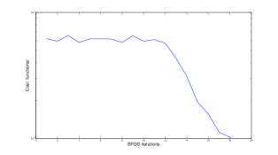
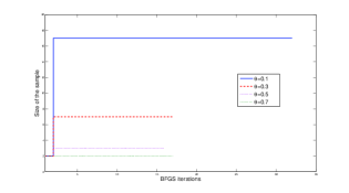
Figure 2 shows two features of Algorithm 1 applied to solve problem (3.1)-(3.2). On the left we represent the evolution of the cost functional along the BFGS iterations. Because of the sampling strategy, in the early iterations of BFGS the problem considered varies quite a lot, thus showing oscillations. Once evolving the process, the convergence is superlinear. On the right we represent the sensitivity with respect to the accuracy parameter $\theta$ (cf. (2.9)): smaller values of $\theta$ penalise larger variances on $\nabla J_{S}$, thus favouring larger samples. Larger values of $\theta$ allow larger variances on $\nabla J_{S}$ and, consequently, smaller sample sizes. In this case, efficiency improves, but accuracy might suffer as shown in Table 3.

Figure 2: Left: evolution of BFGS with Dynamic Sampling along the iterations. Right: samples size changes in Algorithm 1 for different values of $\theta$. For each value of $\theta$, the result is plotted till convergence. For this example $N=20,|S_{0}|=2$.

$\quad\theta\quad$	efficiency	difference
$0.1$	$516$	$0.07\%$
$0.3$	$246$	$4.3\%$
$0.5$	$92$	$5.9\%$
$0.7$	$68$	$15\%$

Table 3: As $\theta$ increases we observe improvements upon the efficiency as smaller samples are allowed. However, the relative difference with the value estimated without sampling shows that accuracy suffers.

Conclusions.

In this paper, we propose an efficient and competitive technique to solve numerically the constrained optimisation problem (1.1)-(1.2) designed for learning the noise model in a TV denoising framework accounting for different types of noise. The set of nonsmooth PDE constraints resembles a large-size training database of clean and noisy images that allows a more robust estimation of parameters. To solve the problem, we use Dynamic Sampling methods, proposed in [3] for linear constrained problems. The idea consists in selecting just a small sample of the PDEs that need to be solved over the whole database and then, during the progression of the algorithm, verify whether such a size produces approximations that are accurate enough. Extended to our nonlinear framework, the results show a remarkable improvement in efficiency, which reflects in reduced computational times for both single noise estimations as well as for mixed ones. Further directions for future research are an accurate analysis of convergence properties of such a scheme as well as the design of a similar algorithm for the case of a $L^{1}$-regularisation on the parameter vector.

Acknowledgements.

This work is supported by the King Abdullah University for Science and Technology (KAUST) Award No. KUK-I1-007-43, the EPSRC first grant Nr. EP/J009539/1 and the Cambridge Center for Analysis (CCA).

References

- [1] Ambrosio, L.; Fusco, N.; Pallara, D.: Functions of Bounded Variation and Free Discontinuity problems, Oxford Mathematical Monographs. Oxford: Clarendon Press. xviii, (2000).
- [2] Bottou, L., Bousquet, O.: The tradeoffs of large scale learning, Advances in Neural Information Processing Systems, 20, 161-168 (2008).
- [3] Byrd R. H., Chin G. M., Nocedal J., Wu Y.: Sample size selection in optimization methods for machine learning, Math. Program. Ser. B, 134, 127-155 (2012).
- [4] Byrd R. H., Chin G. M., Neveitt W., Nocedal J.: On the use of stochastic Hessian information in unconstrained optimisation, SIAM J. Optim., 21(3), 977-995 (2011).
- [5] De Los Reyes J. C., Schönlieb C.-B.:, Image denoising: Learning noise distribution via nonsmooth PDE-constrained optimisation, Inverse Problems and Imaging, vol. 7(4), 1183-1214 (2013).
- [6] Haber E., Chung M., Herrmann F., An effective method for parameter estimation with PDE constraints with multiple right-hand sides, SIAM J. Optim., 22(3), 739-757 (2012).
- [7] Mantle M.D., Sederman A.J., Gladden L.F.: Single- and two- phase flow in fixed-bed reactors: MRI flow visualisation and lattice-Boltzmann simulations, Chemical Engineering Science, 56, 523-529 (2001).
- [8] Nesterov, Y.: Primal-dual subgradient methods for convex problems, Math. Program., 120(1), 221-259 (2009).
- [9] Polyak, B., Juditsky, A.: Acceleration of stochastic approximation by averaging, SIAM J. Control Optim., 30, (1992).
- [10] Robbins, H., Monro, S.: A stochastic approximation method, Ann. Math. Stat., 22(3), 400-407 (1951).