Total Variation Regularisation in Measurement and Image space for PET reconstruction

M Burger1, J Müller2, E Papoutsellis3 and C B Schönlieb3 1Institute for Computational Applied Mathematics and Cells-in-Motion Cluster of Excellence (EXC 1003 CiM), University of Münster, Germany 2Department of Nuclear Medicine, University Hospital Münster 3Department of Applied Mathematics and Theoretical Physics, University of Cambridge martin.burger@wwu.de jahn.mueller@uni-muenster.de ep374@cam.ac.uk cbs31@cam.ac.uk
Abstract

The aim of this paper is to test and analyse a novel technique for image reconstruction in positron emission tomography, which is based on (total variation) regularisation on both the image space and the projection space. We formulate our variational problem considering both total variation penalty terms on the image and on an idealised sinogram to be reconstructed from a given Poisson distributed noisy sinogram. We prove existence, uniqueness and stability results for the proposed model and provide some analytical insight into the structures favoured by joint regularisation.

For the numerical solution of the corresponding discretised problem we employ the split Bregman algorithm and extensively test the approach in comparison to standard total variation regularisation on the image. The numerical results show that an additional penalty on the sinogram performs better on reconstructing images with thin structures.

, , ,

1 Introduction

Positron emission tomography (PET) is a medical imaging technique for studying functional characteristics of the human body, used in brain imaging, neurology, oncology and recently also in cardiology. The patient is injected with a dose of radioactive tracer isotope which concentrates in tissues of interest in the body. Typically, cells in the tissue which are more active have a higher metabolism, i.e., need more energy, and hence will absorb more tracer isotope than cells which are less active. The isotope suffers radioactive decay which invokes it to emit a positron. As soon as the emitted positron meets an electron a pair of gamma rays is sent out into approximately opposite directions and is picked up by the PET-scanner. The collection of all these pairs builds the PET measurement g𝑔g from which the distribution u𝑢u of the relevant radiopharmaceutical shall be reconstructed.

As a (yet simplified) mathematical model the PET measurement can be interpreted as a sample of

f=eLh𝑑tLu𝑑t,𝑓superscript𝑒subscript𝐿differential-d𝑡subscript𝐿𝑢differential-d𝑡f=e^{-\int_{L}h\;dt}\int_{L}u\;dt, (1.1)

where the above integral is the Radon transform \mathcal{R} of u𝑢u along the line L𝐿L connecting the emission point of the gamma rays and the detector, see Figure 1; the above exponential characterises the damping due to the ”attenuation“ function hh (which is, e.g., known from CT [36, Chapter 7]). The function f(L)𝑓𝐿f(L) is called the sinogram of u𝑢u. Since the attenuation can be corrected beforehand we shall ignore the attenuation term in the solution of the inverse problem (corresponding to h00h\equiv 0) in this paper. The basic mathematical problem for the reconstruction of the distribution u𝑢u, is the inversion of the Radon transform. In PET, this inversion is complicated by the presence of undersampling and noise [36]. The PET data usually is corrupted by Poisson noise, also called photon noise, due to the photon counting process during the PET scan.

In this paper, we propose a novel technique for reconstructing an image u𝑢u from noisy PET measurements g𝑔g by a variational regularisation approach using total variation (TV) regularisation [28] on both the image u𝑢u and the sinogram u𝑢\mathcal{R}u. More precisely, let Σn={(θ,s)𝒮n1×}superscriptΣ𝑛𝜃𝑠superscript𝒮𝑛1\Sigma^{n}=\{(\theta,s)\in\mathcal{S}^{n-1}\times\mathbb{R}\} be the projection space (see Figure 1) and 2superscript2\mathbb{R}^{2} the physical space. The Radon transform :L1(2)L1(Σ):superscript𝐿1superscript2superscript𝐿1Σ\mathcal{R}:L^{1}(\mathbb{R}^{2})\rightarrow L^{1}(\Sigma) of uL1(2)𝑢superscript𝐿1superscript2u\in L^{1}(\mathbb{R}^{2}) is given by

u(θ,s)=2u(x)δ(sxθ)𝑑x𝑢𝜃𝑠subscriptsuperscript2𝑢𝑥𝛿𝑠𝑥𝜃differential-d𝑥\mathcal{R}u(\theta,s)=\int_{\mathbb{R}^{2}}u(x)\delta(s-x\cdot\theta)dx (1.2)

Given measurements gL2(Σ)𝑔superscript𝐿2Σg\in L^{2}(\Sigma), we reconstruct uBV(2)𝑢𝐵𝑉superscript2u\in BV(\mathbb{R}^{2}) by solving

argminuBV(2),u0 a.e. in 2{α|Du|(2)+β|D(u)|(Σ)+12Σ(gu)2g}subscriptargminformulae-sequence𝑢𝐵𝑉superscript2𝑢0 a.e. in superscript2𝛼𝐷𝑢superscript2𝛽𝐷𝑢Σ12subscriptΣsuperscript𝑔𝑢2𝑔\operatorname*{arg\,min}_{u\in BV(\mathbb{R}^{2}),~{}u\geq 0\textrm{ a.e. in }\mathbb{R}^{2}}\left\{\alpha|Du|(\mathbb{R}^{2})+\beta|D(\mathcal{R}u)|(\Sigma)+\frac{1}{2}\int_{\Sigma}\frac{(g-\mathcal{R}u)^{2}}{g}\right\} (1.3)

Here BV(2)𝐵𝑉superscript2BV(\mathbb{R}^{2}) is the space of functions of bounded variation, see [2], and α,β𝛼𝛽\alpha,\beta are positive parameters. The terms |Du|(2)𝐷𝑢superscript2|Du|(\mathbb{R}^{2}) and |D(u)|(Σ)𝐷𝑢Σ|D(\mathcal{R}u)|(\Sigma) are TV regularisations on the image u𝑢u and the sinogram u𝑢\mathcal{R}u respectively, that is

|Du|(2)=sup𝐠C0(2;2),g12u𝐠𝑑x,|Du|(Σ)=sup𝐠C0(Σ;2),g1Σu𝐠𝑑x.formulae-sequence𝐷𝑢superscript2subscriptsupremumformulae-sequence𝐠superscriptsubscript𝐶0superscript2superscript2subscriptnorm𝑔1subscriptsuperscript2𝑢𝐠differential-d𝑥𝐷𝑢Σsubscriptsupremumformulae-sequence𝐠superscriptsubscript𝐶0Σsuperscript2subscriptnorm𝑔1subscriptΣ𝑢𝐠differential-d𝑥|Du|(\mathbb{R}^{2})=\sup_{{\bf g}\in C_{0}^{\infty}(\mathbb{R}^{2};\mathbb{R}^{2}),\|g\|_{\infty}\leq 1}\int_{\mathbb{R}^{2}}u~{}\nabla\cdot{\bf g}~{}dx,\quad|D\mathcal{R}u|(\Sigma)=\sup_{{\bf g}\in C_{0}^{\infty}(\Sigma;\mathbb{R}^{2}),\|g\|_{\infty}\leq 1}\int_{\Sigma}\mathcal{R}u~{}\nabla\cdot{\bf g}~{}dx.

The data fidelity Σ(gu)2/gsubscriptΣsuperscript𝑔𝑢2𝑔\int_{\Sigma}(g-\mathcal{R}u)^{2}/g is a weighted L2superscript𝐿2L^{2} norm that constitutes a standard approximation of the Poisson noise model given by the Kullback-Leibler divergence, compare [29, Chapter 4] for instance.

Refer to caption
Fig. 1: PET scan geometry. The image function u𝑢u is encoded in integrals f(L)=f(θ,s)𝑓𝐿𝑓𝜃𝑠f(L)=f(\theta,s) along lines L𝐿L from the emission point to the detectors, cf. (1.1). The lines L𝐿L are defined by an angle θ𝜃\theta and distance s𝑠s to the origin. (Lsuperscript𝐿L^{{}^{\prime}} is the distance from the emission point through the object.)

PET reconstruction using TV regularisation is not new. However, typically the TV regularisation is applied to the image function u𝑢u only. By additionally regularising the sinogram u𝑢\mathcal{R}u using a total variation penalty in projection space we will show that under certain conditions images of higher quality can be reconstructed. In particular, this is the case in the presence of high noise in g𝑔g and when aiming to preserve thin and elongated structures in u𝑢u.

1.1 Related methods

Our approach (1.3) is inspired by an alternating regularisation procedure for PET first introduced by Barbano et al. in [3]. Given possible under sampled and noisy PET measurements gn×m𝑔superscript𝑛𝑚g\in\mathbb{R}^{n\times m} an image usuperscript𝑢u^{*} is reconstructed by solving

min{(s,u):sn×m,u=1s}αs1+βu1+λ2gs22,subscriptconditional-set𝑠𝑢formulae-sequence𝑠superscript𝑛𝑚𝑢superscript1𝑠𝛼subscriptdelimited-∥∥𝑠1𝛽subscriptdelimited-∥∥𝑢1𝜆2superscriptsubscriptdelimited-∥∥𝑔𝑠22\min_{\{(s,u):~{}s\in\mathbb{R}^{n\times m},u=\mathcal{R}^{-1}s\}}\alpha\left\lVert\nabla s\right\rVert_{1}+\beta\left\lVert u\right\rVert_{1}+\frac{\lambda}{2}\left\lVert g-s\right\rVert_{2}^{2}, (1.4)

where 1superscript1\mathcal{R}^{-1} is the inverse Radon transform approximated by the filtered backprojection and α,β𝛼𝛽\alpha,\beta and λ𝜆\lambda are positive weighting parameters. Note that here a regularised reconstruction usuperscript𝑢u^{*} is computed by smoothing both the image u𝑢u and the sinogram s𝑠s. Indeed, the regularisation in (1.4) is given by the total variation regulariser s1subscriptdelimited-∥∥𝑠1\left\lVert\nabla s\right\rVert_{1}, see [28], that acts on the sinogram s𝑠s only. The image u𝑢u is forced to be sparse by an 1subscript1\ell_{1} penalty. The main focus of [3] is to study the effect of total variation regularisation on the sinogram, rather than the image as usually done in variational PET reconstruction [31, 30, 10, 11]. Therefore, in their numerical experiment the effect of the image regularisation is kept low by choosing an appropriate weighting αβmuch-greater-than𝛼𝛽\alpha\gg\beta. In [3] it is proved that (1.4) has a unique solution (s,u)superscript𝑠superscript𝑢(s^{*},u^{*}). Moreover, the authors show the effect, the total variation regularisation of the sinogram s𝑠s, has on the reconstructed image u𝑢u by a computational experiment on a simulated data set.

The main idea of adding an total variation regularisation on the projection space originated in the works of Thirion [34], and Prince et al. [27]. In [34] the author proposes to connect edge detection of the tomographic image to finding continuous lines in the sinogram. That is, a point on a line in the sinogram corresponds to an edge in the object space with a fixed orientation and distance from the origin, see Figure 1. Moreover, in [27] Prince and Willsky focus on reconstructing tomographic images by using a Markov random field prior on the sinogram, in particular in the presence of data with a low signal-to-noise ratio (SNR) and limited angle or sparse-angle measurement configurations. Their approach leads to the computation of a smoothed sinogram from which the image u𝑢u is reconstructed using filtered back projection.

1.2 State of the art - direct and iterative PET reconstruction

In (1.3) we reconstruct an image from PET measurements by smoothing both in measurement and image space. This indeed combines the philosophies of the two main approaches for image reconstruction from PET measurements: (i) Direct methods and (ii) iterative / variational method. While in direct methods the PET measurements are smoothed by an appropriate filter and then inverted (cf. e.g. [24, 22]), iterative methods (respectively variational methods solved iteratively) are based on the standard Bayesian modelling approach in inverse problems in which prior knowledge in terms of regularity is expressed for the image function u𝑢u (rather than the measurements f𝑓f). The possibility to include statistical noise models is a main advantage of iterative and variational methods, on which we shall focus in the following.

In iterative methods for PET reconstruction the noise distribution is accounted for by modelling the randomness in the numbers of detected gamma counts. The most popular iterative approach for PET reconstruction is the expectation-maximization (EM) algorithm. To recall, the problem of image reconstruction can be formulated as a solution of the linear and ill-conditioned operator equation:

g=Ku𝑔𝐾𝑢g=Ku

where g𝑔g is the Poisson distributed data and K𝐾K is a finite-dimensional sampling of the Radon transform. Typically, we may assume that the data are realizations of random variables Xisubscript𝑋𝑖X_{i} and we consider the detected values gisubscript𝑔𝑖g_{i} as a realization of a random variable Xisubscript𝑋𝑖X_{i}, for i=1,,N𝑖1𝑁i=1,...,N. It is reasonable to maximize the conditional probability P(u|g)𝑃conditional𝑢𝑔P(u|g), which by the Bayes’ Law is:

P(u|g)=P(g|u)P(u)P(g)𝑃conditional𝑢𝑔𝑃conditional𝑔𝑢𝑃𝑢𝑃𝑔P(u|g)=\frac{P(g|u)P(u)}{P(g)}

It is equivalent to maximize P(g|u)P(u)𝑃conditional𝑔𝑢𝑃𝑢P(g|u)P(u), since the denominator does not depend on u𝑢u. Moreover, the random variables of the measured data are Poisson distributed with expected values given by (Ku)isubscript𝐾𝑢𝑖(Ku)_{i} and

P(g|u)=i=1N(Ku)igigi!e(Ku)i𝑃conditional𝑔𝑢superscriptsubscriptproduct𝑖1𝑁superscriptsubscript𝐾𝑢𝑖subscript𝑔𝑖subscript𝑔𝑖superscript𝑒subscript𝐾𝑢𝑖P(g|u)=\prod_{i=1}^{N}\frac{(Ku)_{i}^{g_{i}}}{g_{i}!}e^{-(Ku)_{i}} (1.5)

The Bayesian approach allows to consider additional information to our model with an appropriate prior probability of the image u𝑢u, see [15], [21]. The most frequently used prior densities are the Gibbs priors, i.e.,

P(u)=eαJ(u)𝑃𝑢superscript𝑒𝛼𝐽𝑢P(u)=e^{-\alpha J(u)} (1.6)

where α>0𝛼0\alpha>0 is a regularisation parameter and J(u)𝐽𝑢J(u) is a convex energy functional. Instead of maximising P(g|u)P(u)𝑃conditional𝑔𝑢𝑃𝑢P(g|u)P(u), we minimise log(P(g|u)P(u))𝑃conditional𝑔𝑢𝑃𝑢-\log(P(g|u)P(u)). Hence, we seek a minimiser of the following problem

argminu0{i=1N((Ku)igilog(Ku)i)+αJ(u)},\operatorname*{arg\,min}_{u\geq 0}\left\{\sum_{i=1}^{N}((Ku)_{i}-g_{i}\log(Ku)_{i})+\alpha J(u)\right\}, (1.7)

where the first term is the so-called Kullback-Leibler divergence of u𝑢u and g𝑔g. This often serves as a motivation to consider the continuous variational problem

argminu0{(Kuglog(Ku))+αJ(u)}subscriptargmin𝑢0𝐾𝑢𝑔𝐾𝑢𝛼𝐽𝑢\operatorname*{arg\,min}_{u\geq 0}\left\{\int(Ku-g\log(Ku))+\alpha J(u)\right\} (1.8)

In the case where J0𝐽0J\equiv 0, the first optimality condition in (1.8) yields the following iterative scheme, known as EM algorithm

uk+1=ukK1K(gKuk)superscript𝑢𝑘1superscript𝑢𝑘superscript𝐾1superscript𝐾𝑔𝐾subscript𝑢𝑘u^{k+1}=\frac{u^{k}}{K^{*}1}K^{*}(\frac{g}{Ku_{k}})

Additionally imposing prior information on the solution, e.g., that the solutions has a small total variation, leads to an extension of the EM algorithm, e.g., the EM-TV algorithm [4, 10]. See also [31, 30, 5, 37] for related approaches and [10, 11] for extensions of EM-TV to Bregmanized total variation regularization.

Outline

The rest of the paper is organised as follows: in the next section we prove existence, uniqueness and stability results for our variational model in the continuous setting. In section 3, we focus on solving numerically our problem using the split Bregman method and present our numerical simulations in section 4.

2 TV regularisation on image and sinogram

In this section, we will discuss the well-posedness of our minimisation problem (1.3). To do so, we first rewrite (1.3) for image functions u𝑢u that are defined on a bounded and open domain Ω2Ωsuperscript2\Omega\subset\mathbb{R}^{2} including sufficiently large balls around zero. We consider the following problem

argminuBV(Ω),u0 a.e. in Ω{F(u)=α|Du|(Ω)+β|D(u)|(Σ)+12Σ(gu)2g}subscriptargminformulae-sequence𝑢𝐵𝑉Ω𝑢0 a.e. in Ω𝐹𝑢𝛼𝐷𝑢Ω𝛽𝐷𝑢Σ12subscriptΣsuperscript𝑔𝑢2𝑔\operatorname*{arg\,min}_{u\in BV(\Omega),~{}u\geq 0\textrm{ a.e. in }\Omega}\left\{F(u)=\alpha|Du|(\Omega)+\beta|D(\mathcal{R}u)|(\Sigma)+\frac{1}{2}\int_{\Sigma}\frac{(g-\mathcal{R}u)^{2}}{g}\right\} (2.1)

We enforce prior information in terms of regularisation on both the image and its sinogram. Note, that the TV regularisation on the sinogram in (2.1) has a different effect on the reconstructed image compared to regularising in image space (β=0𝛽0\beta=0) only. Of course, regularisation of the image u𝑢u enforces a certain regularisation of the sinogram u𝑢\mathcal{R}u as well. However, because of the nonlinear character of the total variation regularisation, TV regularisation of the sinogram is not equivalent to regularisation on the image and vice-versa. In (2.1) the two types of TV regularisation impose different structures in the subgradients of the two terms. This is also emphasised in Section 2.4 where the source condition (2.22) and the elements p1,p2subscript𝑝1subscript𝑝2p_{1},p_{2} are described. Indeed, beyond the topology imposed by the regulariser the structure imposed by the sub gradients of the total variation regularisers are crucial for the properties of a solution of (2.1). In particular, in what follows we will see that the additional TV regularisation on the sinogram can have a positive effect when reconstructing smooth, thin structures as can be observed in the myocardium for instance. This effect will be both motivated analytically by the characterisation of a solution of (2.1) for the simple case when g𝑔g is the sinogram of a disc for instance, as well as experimentally verified by testing the method against some representative examples in the numerical part of the paper.

We start with some first observations that are crucial ingredients of the well-posedness analysis for (2.1). In order not to divide by zero in the weighted L2superscript𝐿2L^{2} norm in (2.1), we first assume that there exists constant c1>0subscript𝑐10c_{1}>0 such that

0<c1g(θ,s)gL(Σ)0subscript𝑐1𝑔𝜃𝑠subscriptdelimited-∥∥𝑔superscript𝐿Σ0<c_{1}\leq g(\theta,s)\leq\left\lVert g\right\rVert_{L^{\infty}(\Sigma)} (2.2)

The constraint (2.2) is not significantly restrictive in most medical experiments. Since u𝑢u is assumed to be nonnegative, this basically can be achieved if the lines in the Radon transform are confined to those intersecting the support of u𝑢u, at least in a discretised setting.

Moreover, to justify the definition of F(u)𝐹𝑢F(u) in (2.1) over the admissible set {uBV(Ω),u0 a.e. in Ω}formulae-sequence𝑢𝐵𝑉Ω𝑢0 a.e. in Ω\{u\in BV(\Omega),~{}u\geq 0\textrm{ a.e. in }\Omega\} in Theorem 2.1 we show that the Radon transform of u𝑢u is again in BV𝐵𝑉BV. To do so it is important to assume that the object we wish to recover is compactly supported. Hence, we may assume that suppuBrΩsupp𝑢subscript𝐵𝑟Ω{\rm supp}~{}u\subset B_{r}\subset\Omega, where Brsubscript𝐵𝑟B_{r} is the ball with radius r centered at the origin. Consequently, (1.2) implies that u(θ,s)=0𝑢𝜃𝑠0\mathcal{R}u(\theta,s)=0, when s[r,r]𝑠𝑟𝑟s\notin[-r,r] and the projection space becomes:

Σ={(θ,s):rsr,0θ<π}Σconditional-set𝜃𝑠formulae-sequence𝑟𝑠𝑟0𝜃𝜋\Sigma=\left\{(\theta,s):-r\leq s\leq r,0\leq\theta<\pi\right\} (2.3)

If it is not stated otherwise, we will always assume that the reconstructed image is compactly supported. Note that, we allow negative values on the s variable and that we do not consider the Radon transform for θ=π𝜃𝜋\theta=\pi. Likewise, we may allow that s0𝑠0s\geq 0 and 0θ<2π0𝜃2𝜋0\leq\theta<2\pi. Hence, we consider the Radon space ΣΣ\Sigma as the surface of a half cylinder with radius 1. Moreover, since Dirac δ𝛿\delta function is even, equation (1.2) implies that the coordinates (s,ϕ𝑠italic-ϕ-s,\phi) and (s,ϕ+π𝑠italic-ϕ𝜋s,\phi+\pi) correspond to the same point in the Radon space.

2.1 BV-continuity of the Radon transform

Our first result deals with a continuity property for the Radon transform as a mapping operator for functions with bounded variation. A similar result is proved by M. Bergounioux and E. Trélat [8] in the three dimensional case and for bounded and axially symmetric objects. In what follows we do not need this symmetry assumption, but prove that the Radon transform is BV continuous for compactly supported u𝑢u in two space dimensions.

Theorem 2.1.

Let uBV(Ω)𝑢𝐵𝑉Ωu\in BV(\Omega) and the ball Brsubscript𝐵𝑟B_{r} with radius r be its compact support, then uBV(Σ)𝑢𝐵𝑉Σ\mathcal{R}u\in BV(\Sigma) and the Radon transform is BV continuous on the subspace of functions supported in Brsubscript𝐵𝑟B_{r}.

Proof.

It is well known that the Radon transform is L1 continuous and the following estimate holds for n2𝑛2n\geq 2:

uL1(Σn)|Sn1|uL1(n)subscriptdelimited-∥∥𝑢superscript𝐿1superscriptΣ𝑛superscript𝑆𝑛1subscriptdelimited-∥∥𝑢superscript𝐿1superscript𝑛\left\lVert\mathcal{R}u\right\rVert_{L^{1}(\Sigma^{n})}\leq|S^{n-1}|\left\lVert u\right\rVert_{L^{1}(\mathbb{R}^{n})} (2.4)

Hence, to prove BV-continuity we need to prove that the variation of u𝑢\mathcal{R}u over ΣΣ\Sigma is finite and bounded by the BV norm of u𝑢u, i.e.,

V(u,Σ)=sup{Ωu(θ,s)divg(θ,s)𝑑θ𝑑s: g(Cc1(Σ))2 , g1}<𝑉𝑢Σsupremumconditional-setsubscriptΩ𝑢𝜃𝑠div𝑔𝜃𝑠differential-d𝜃differential-d𝑠 𝑔superscriptsubscriptsuperscript𝐶1𝑐Σ2 , subscriptdelimited-∥∥𝑔1V(\mathcal{R}u,\Sigma)=\sup\left\{\int_{\Omega}\mathcal{R}u(\theta,s){\rm div}g(\theta,s)d\theta ds:\mbox{ }g\in(C^{1}_{c}(\Sigma))^{2}\mbox{ , }\left\lVert g\right\rVert_{\infty}\leq 1\right\}<\infty

The following equations can easily be derived by the geometry depicted in Figure 1, where (x,y)𝑥𝑦(x,y) is the annihilation point and t𝑡t runs through the line L𝐿L:

x=scosθtsinθ𝑥𝑠𝜃𝑡𝜃\displaystyle x=s\cos\theta-t\sin\theta (2.5)
y=ssinθ+tcosθ𝑦𝑠𝜃𝑡𝜃\displaystyle y=s\sin\theta+t\cos\theta (2.6)

We may also assume that t[r,r]𝑡𝑟𝑟t\in[-r,r]. Therefore,

Ωu(θ,s)divg(θ,s)𝑑θ𝑑ssubscriptΩ𝑢𝜃𝑠div𝑔𝜃𝑠differential-d𝜃differential-d𝑠\displaystyle\int_{\Omega}\mathcal{R}u(\theta,s){\rm div}g(\theta,s)d\theta ds =0πrrrru(scosθtsinθ,ssinθ+tcosθ)absentsuperscriptsubscript0𝜋superscriptsubscript𝑟𝑟superscriptsubscript𝑟𝑟𝑢𝑠𝜃𝑡𝜃𝑠𝜃𝑡𝜃\displaystyle=\int_{0}^{\pi}\int_{-r}^{r}\int_{-r}^{r}u(s\cos\theta-t\sin\theta,s\sin\theta+t\cos\theta)
divg(θ,s) dtdsdθdiv𝑔𝜃𝑠 𝑑𝑡𝑑𝑠𝑑𝜃\displaystyle{\rm div}g(\theta,s)\mbox{ }dtdsd\theta
=0πrrrru(x,y)[g1α+g2θ]𝑑x𝑑y𝑑θabsentsuperscriptsubscript0𝜋superscriptsubscript𝑟𝑟superscriptsubscript𝑟𝑟𝑢𝑥𝑦delimited-[]subscript𝑔1𝛼subscript𝑔2𝜃differential-d𝑥differential-d𝑦differential-d𝜃\displaystyle=\int_{0}^{\pi}\int_{-r}^{r}\int_{-r}^{r}u(x,y)\left[\nabla g_{1}\cdot\vec{\alpha}+\nabla g_{2}\cdot\vec{\theta}\right]dxdyd\theta

where α=(y,x)𝛼𝑦𝑥\vec{\alpha}=(-y,x), θ=(cosθ,sinθ)𝜃𝜃𝜃\vec{\theta}=(\cos\theta,\sin\theta) and in the above calculations we have used equations (2.5),(2.6). Define, G(x,y)=(G1(x,y),G2(x,y)))\vec{G}(x,y)=(G_{1}(x,y),G_{2}(x,y))) with

G1(x,y)subscript𝐺1𝑥𝑦\displaystyle G_{1}(x,y) =0πyg1(θ,xcosθ+ysinθ)+g2(θ,xcosθ+ysinθ)cosθdθabsentsuperscriptsubscript0𝜋𝑦subscript𝑔1𝜃𝑥𝜃𝑦𝜃subscript𝑔2𝜃𝑥𝜃𝑦𝜃𝜃𝑑𝜃\displaystyle=\int_{0}^{\pi}-yg_{1}(\theta,x\cos\theta+y\sin\theta)+g_{2}(\theta,x\cos\theta+y\sin\theta)\cos\theta d\theta
G2(x,y)subscript𝐺2𝑥𝑦\displaystyle G_{2}(x,y) =0πxg1(θ,xcosθ+ysinθ)+g2(θ,xcosθ+ysinθ)sinθdθabsentsuperscriptsubscript0𝜋𝑥subscript𝑔1𝜃𝑥𝜃𝑦𝜃subscript𝑔2𝜃𝑥𝜃𝑦𝜃𝜃𝑑𝜃\displaystyle=\int_{0}^{\pi}xg_{1}(\theta,x\cos\theta+y\sin\theta)+g_{2}(\theta,x\cos\theta+y\sin\theta)\sin\theta d\theta

then,

divG(x,y)=g1x+g2y=0π(g1α+g2θ)𝑑θdiv𝐺𝑥𝑦subscript𝑔1𝑥subscript𝑔2𝑦superscriptsubscript0𝜋subscript𝑔1𝛼subscript𝑔2𝜃differential-d𝜃{\rm div}G(x,y)=\frac{\partial g_{1}}{\partial x}+\frac{\partial g_{2}}{\partial y}=\int_{0}^{\pi}\left(\nabla g_{1}\cdot\vec{\alpha}+\nabla g_{2}\cdot\vec{\theta}\right)d\theta

The function G𝐺G lies in C1(2)superscript𝐶1superscript2C^{1}(\mathbb{R}^{2}) and if we restrict G𝐺G on ΩΩ\Omega and consider GχBr𝐺subscript𝜒subscript𝐵𝑟G\chi_{B_{r}} then GCc1(Ω)𝐺superscriptsubscript𝐶𝑐1ΩG\in C_{c}^{1}(\Omega). Moreover,

|G1(x,y)|0π|y||g1|+|g2|πg(1+|y|)πg(1+r)=Csubscript𝐺1𝑥𝑦superscriptsubscript0𝜋𝑦subscript𝑔1subscript𝑔2𝜋subscriptdelimited-∥∥𝑔1𝑦𝜋subscriptdelimited-∥∥𝑔1𝑟𝐶|G_{1}(x,y)|\leq\int_{0}^{\pi}|y||g_{1}|+|g_{2}|\leq\pi\left\lVert g\right\rVert_{\infty}(1+|y|)\leq\pi\left\lVert g\right\rVert_{\infty}(1+r)=C

and |G2(x,y)|Csubscript𝐺2𝑥𝑦𝐶|G_{2}(x,y)|\leq C. If we set

A=rrrru(x,y)divG(x,y)𝑑x𝑑y=Crrrru(x,y)div(G(x,y)C)𝑑x𝑑y𝐴superscriptsubscript𝑟𝑟superscriptsubscript𝑟𝑟𝑢𝑥𝑦div𝐺𝑥𝑦differential-d𝑥differential-d𝑦𝐶superscriptsubscript𝑟𝑟superscriptsubscript𝑟𝑟𝑢𝑥𝑦div𝐺𝑥𝑦𝐶differential-d𝑥differential-d𝑦A=\int_{-r}^{r}\int_{-r}^{r}u(x,y){\rm div}G(x,y)dxdy=C\int_{-r}^{r}\int_{-r}^{r}u(x,y){\rm div}(\frac{G(x,y)}{C})dxdy

and

B=Σu(θ,s)divg(θ,s)𝑑s𝑑θ𝐵subscriptΣ𝑢𝜃𝑠div𝑔𝜃𝑠differential-d𝑠differential-d𝜃B=\int_{\Sigma}\mathcal{R}u(\theta,s){\rm div}g(\theta,s)dsd\theta

then, taking the supremum over all GCc1(Ω)𝐺superscriptsubscript𝐶𝑐1ΩG\in C_{c}^{1}(\Omega) with G/C1subscriptdelimited-∥∥𝐺𝐶1\left\lVert G/C\right\rVert_{\infty}\leq 1, we have that B=CV(u,Ω)𝐵𝐶𝑉𝑢ΩB=C\cdot V(u,\Omega). Similarly, for all g(Cc1(Σ))2𝑔superscriptsuperscriptsubscript𝐶𝑐1Σ2g\in(C_{c}^{1}(\Sigma))^{2} with g1subscriptdelimited-∥∥𝑔1\left\lVert g\right\rVert_{\infty}\leq 1, we conclude that

V(u,Σ)π(1+r)V(u,Ω)<𝑉𝑢Σ𝜋1𝑟𝑉𝑢ΩV(\mathcal{R}u,\Sigma)\leq\pi(1+r)V(u,\Omega)<\infty

Therefore, uBV(Σ)𝑢𝐵𝑉Σ\mathcal{R}u\in BV(\Sigma) and the variation coincides with the total variation |D(u)|(Σ)𝐷𝑢Σ|D(\mathcal{R}u)|(\Sigma). By the corresponding norm defined on the BV space and equation (2.4), we deduce that

uBV(Σ)π(1+r)uBV(Ω).subscriptdelimited-∥∥𝑢𝐵𝑉Σ𝜋1𝑟subscriptdelimited-∥∥𝑢𝐵𝑉Ω\left\lVert\mathcal{R}u\right\rVert_{BV(\Sigma)}\leq\pi(1+r)\left\lVert u\right\rVert_{BV(\Omega)}.

2.2 Existence and Uniqueness

Next, we show existence and uniqueness of the minimiser for the problem (2.1).

Theorem 2.2.

Let α>0𝛼0\alpha>0, β0𝛽0\beta\geq 0 and gL(Σ)𝑔superscript𝐿Σg\in L^{\infty}(\Sigma) a strictly positive function. Then the functional F(u)𝐹𝑢F(u) in (2.1) is lower semicontinuous and strictly convex and the minimisation problem (2.1) attains a unique solution uBV(Ω)L+1(Ω)𝑢𝐵𝑉Ωsuperscriptsubscript𝐿1Ωu\in BV(\Omega)\cap L_{+}^{1}(\Omega).

Proof.

Let (un)nBV(Ω)subscriptsubscript𝑢𝑛𝑛𝐵𝑉Ω(u_{n})_{n}\in BV(\Omega) be a minimising sequence of nonnegative functions, then in particular there exists a constant C1>0subscript𝐶10C_{1}>0 such that

F(u)=α|Dun|(Ω)+β|D(un)|(Σ)+12Σ(gun)2g<C1𝐹𝑢𝛼𝐷subscript𝑢𝑛Ω𝛽𝐷subscript𝑢𝑛Σ12subscriptΣsuperscript𝑔subscript𝑢𝑛2𝑔subscript𝐶1F(u)=\alpha|Du_{n}|(\Omega)+\beta|D(\mathcal{R}u_{n})|(\Sigma)+\frac{1}{2}\int_{\Sigma}\frac{(g-\mathcal{R}u_{n})^{2}}{g}<C_{1} (2.7)

Let un¯=1|Ω|Ωun𝑑x¯subscript𝑢𝑛1ΩsubscriptΩsubscript𝑢𝑛differential-d𝑥\overline{u_{n}}=\frac{1}{|\Omega|}\int_{\Omega}u_{n}dx, then by the Poincaré-Wirtinger inequality [2], we can find a constant C2>0subscript𝐶20C_{2}>0 such that

unun¯L2(Ω)C2|Dun|(Ω)subscriptdelimited-∥∥subscript𝑢𝑛¯subscript𝑢𝑛superscript𝐿2Ωsubscript𝐶2𝐷subscript𝑢𝑛Ω\left\lVert u_{n}-\overline{u_{n}}\right\rVert_{L^{2}(\Omega)}\leq C_{2}|Du_{n}|(\Omega) (2.8)

Therefore

unL2(Ω)C2|Dun|(Ω)+|Ωun𝑑x|subscriptdelimited-∥∥subscript𝑢𝑛superscript𝐿2Ωsubscript𝐶2𝐷subscript𝑢𝑛ΩsubscriptΩsubscript𝑢𝑛differential-d𝑥\left\lVert u_{n}\right\rVert_{L^{2}(\Omega)}\leq C_{2}|Du_{n}|(\Omega)+|\int_{\Omega}u_{n}dx|

Following the proof of [35], we set vn=unun¯subscript𝑣𝑛subscript𝑢𝑛¯subscript𝑢𝑛v_{n}=u_{n}-\overline{u_{n}} and since

C1subscript𝐶1\displaystyle C_{1} Σ(gun)2g1gL(Σ)gunL2(Σ)2absentsubscriptΣsuperscript𝑔subscript𝑢𝑛2𝑔1subscriptdelimited-∥∥𝑔superscript𝐿Σsuperscriptsubscriptdelimited-∥∥𝑔subscript𝑢𝑛superscript𝐿2Σ2\displaystyle\geq\int_{\Sigma}\frac{(g-\mathcal{R}u_{n})^{2}}{g}\geq\frac{1}{\left\lVert g\right\rVert_{L^{\infty}(\Sigma)}}\left\lVert g-\mathcal{R}u_{n}\right\rVert_{L^{2}(\Sigma)}^{2}

one can prove that

un¯L2(Σ)subscriptdelimited-∥∥¯subscript𝑢𝑛superscript𝐿2Σ\displaystyle\left\lVert\mathcal{R}\overline{u_{n}}\right\rVert_{L^{2}(\Sigma)} C1gL(Σ)+vnL2(Σ)+gL2(Σ)absentsubscript𝐶1subscriptdelimited-∥∥𝑔superscript𝐿Σsubscriptdelimited-∥∥subscript𝑣𝑛superscript𝐿2Σsubscriptdelimited-∥∥𝑔superscript𝐿2Σ\displaystyle\leq C_{1}\left\lVert g\right\rVert_{L^{\infty}(\Sigma)}+\left\lVert\mathcal{R}v_{n}\right\rVert_{L^{2}(\Sigma)}+\left\lVert g\right\rVert_{L^{2}(\Sigma)}
C1~gL(Σ)+vnL2(Σ)absent~subscript𝐶1subscriptdelimited-∥∥𝑔superscript𝐿Σsubscriptdelimited-∥∥subscript𝑣𝑛superscript𝐿2Σ\displaystyle\leq\widetilde{C_{1}}\left\lVert g\right\rVert_{L^{\infty}(\Sigma)}+\left\lVert\mathcal{R}v_{n}\right\rVert_{L^{2}(\Sigma)}

and

|1|Ω|Ωun𝑑x|χΩL2(Σ)=un¯L2(Σ)1ΩsubscriptΩsubscript𝑢𝑛differential-d𝑥subscriptdelimited-∥∥subscript𝜒Ωsuperscript𝐿2Σsubscriptdelimited-∥∥¯subscript𝑢𝑛superscript𝐿2Σ|\frac{1}{|\Omega|}\int_{\Omega}u_{n}dx|\cdot\left\lVert\mathcal{R}\chi_{\Omega}\right\rVert_{L^{2}(\Sigma)}=\left\lVert\mathcal{R}\overline{u_{n}}\right\rVert_{L^{2}(\Sigma)}

Without loss of generality, we may assume that the image domain ΩΩ\Omega is a unit square, then χΩ0subscript𝜒Ω0\mathcal{R}\chi_{\Omega}\neq 0, see [26, Chapter 8] and we conclude that |Ωun𝑑x|subscriptΩsubscript𝑢𝑛differential-d𝑥|\int_{\Omega}u_{n}dx| is uniformly bounded. Hence, unsubscript𝑢𝑛u_{n} is L1(Ω)superscript𝐿1ΩL^{1}(\Omega) bounded ( L2(Ω)superscript𝐿2ΩL^{2}(\Omega) bounded with |Ω|<Ω|\Omega|<\infty). Moreover, since the Radon transform is L2superscript𝐿2L^{2} continuous for functions with compact support (cf. [20],[24]) and using (2.4), we have the following:

Since, (un)nsubscriptsubscript𝑢𝑛𝑛(u_{n})_{n\in\mathbb{N}} is bounded in L1(Ω)superscript𝐿1ΩL^{1}(\Omega) and |Dun|(Ω)<𝐷subscript𝑢𝑛Ω|Du_{n}|(\Omega)<\infty i.e., is BV(Ω)𝐵𝑉ΩBV(\Omega) bounded, we obtain a subsequence (unk)k,uBV(Ω)subscriptsubscript𝑢subscript𝑛𝑘𝑘𝑢𝐵𝑉Ω(u_{n_{k}})_{k\in\mathbb{N}},u\in BV(\Omega) such that unksubscript𝑢subscript𝑛𝑘u_{n_{k}} converges weakly to u. Also, unksubscript𝑢subscript𝑛𝑘u_{n_{k}} converges weakly to u in L2(Ω)superscript𝐿2ΩL^{2}(\Omega). Then,

unku in L1(Σ)subscript𝑢subscript𝑛𝑘𝑢 in superscript𝐿1Σ\displaystyle\mathcal{R}u_{n_{k}}\rightarrow\mathcal{R}u\mbox{ in }L^{1}(\Sigma) (2.9)
unku in L2(Σ)subscript𝑢subscript𝑛𝑘𝑢 in superscript𝐿2Σ\displaystyle\mathcal{R}u_{n_{k}}\rightharpoonup\mathcal{R}u\mbox{ in }L^{2}(\Sigma) (2.10)

Then,

|D(u)|(Σ)lim infk|D(unk)|(Σ)𝐷𝑢Σsubscriptlimit-infimum𝑘𝐷subscript𝑢subscript𝑛𝑘Σ|D(\mathcal{R}u)|(\Sigma)\leq\liminf_{k\rightarrow\infty}|D(\mathcal{R}u_{n_{k}})|(\Sigma)

and the weak lower semicontinuity of the L2superscript𝐿2L^{2} norm and the lower semicontinuity of total variation semi-norm for both the image and the projection space imply that

F(u)lim infkF(unk)𝐹𝑢subscriptlimit-infimum𝑘𝐹subscript𝑢subscript𝑛𝑘F(u)\leq\liminf_{k\rightarrow\infty}F(u_{n_{k}})

To prove uniqueness let 0u1,u2BV(Ω)formulae-sequence0subscript𝑢1subscript𝑢2𝐵𝑉Ω0\leq u_{1},u_{2}\in BV(\Omega) be two minimisers. If u1u2subscript𝑢1subscript𝑢2\mathcal{R}u_{1}\neq\mathcal{R}u_{2}, then the strict convexity of the weighted L2superscript𝐿2L^{2} fidelity term together with the convexity of the total variation of u𝑢\mathcal{R}u implies that:

F(u1+u22)<F(u1)2+F(u2)2=infuBV(Ω)u0a.e.F(u)𝐹subscript𝑢1subscript𝑢22𝐹subscript𝑢12𝐹subscript𝑢22subscriptinfimum𝑢𝐵𝑉Ω𝑢0a.e.𝐹𝑢F\left(\frac{u_{1}+u_{2}}{2}\right)<\frac{F(u_{1})}{2}+\frac{F(u_{2})}{2}=\inf_{\begin{subarray}{c}u\in BV(\Omega)\\ u\geq 0\mbox{a.e.}\end{subarray}}F(u)

which is a contradiction. Hence, u1=u2subscript𝑢1subscript𝑢2\mathcal{R}u_{1}=\mathcal{R}u_{2} and using the well-known Slice-Projection theorem i.e.,

(θu(s))=(2π)n12n(u(sθ))subscript𝜃𝑢𝑠superscript2𝜋𝑛12subscript𝑛𝑢𝑠𝜃\mathcal{F}(\mathcal{R}_{\theta}u(s))=(2\pi)^{\frac{n-1}{2}}\mathcal{F}_{n}(u(s\theta))

where the right hand side denotes the n-dimensional Fourier transform, we conclude that u1=u2subscript𝑢1subscript𝑢2u_{1}=u_{2}, see also [23], [24] for more details.

2.3 Stability

Further, we discuss the stability of problem (2.1) in terms of a small perturbation on the data. Following the approach of Acar and Vogel in [1], we consider a perturbation on the projection space i.e.,

gn=g+τn with τnL2(Σ)0subscript𝑔𝑛𝑔subscript𝜏𝑛 with subscriptdelimited-∥∥subscript𝜏𝑛superscript𝐿2Σ0g_{n}=g+\tau_{n}\mbox{ with }\left\lVert\tau_{n}\right\rVert_{L^{2}(\Sigma)}\rightarrow 0 (2.11)

and define the corresponding minimisation problem on the perturbed functionals:

argminu0 a.e, 
u
BV(Ω)
{Fn(u)=α|Du|(Ω)+β|D(u)|(Σ)+12Σ(gnu)2gn}
subscriptargmin𝑢0 a.e, 
𝑢
𝐵𝑉Ω
superscript𝐹𝑛𝑢𝛼𝐷𝑢Ω𝛽𝐷𝑢Σ12subscriptΣsuperscriptsubscript𝑔𝑛𝑢2subscript𝑔𝑛
\operatorname*{arg\,min}_{u\geq 0\mbox{ a.e, }\\ u\in BV(\Omega)}\left\{F^{n}(u)=\alpha|Du|(\Omega)+\beta|D(\mathcal{R}u)|(\Sigma)+\frac{1}{2}\int_{\Sigma}\frac{(g_{n}-\mathcal{R}u)^{2}}{g_{n}}\right\}
(2.12)

For (2.12) to be well-defined we assume an Lsuperscript𝐿L^{\infty} bound on τnsubscript𝜏𝑛\tau_{n} such that gnsubscript𝑔𝑛g_{n} is still positive. More precisely we assume that

0<c1gn(θ,s)gL(Σ)+ε, for all n1,0subscript𝑐1subscript𝑔𝑛𝜃𝑠subscriptdelimited-∥∥𝑔superscript𝐿Σ𝜀, for all 𝑛10<c_{1}\leq g_{n}(\theta,s)\leq\left\lVert g\right\rVert_{L^{\infty}(\Sigma)}+\varepsilon\mbox{, for all }n\geq 1, (2.13)

which is the same as assuming that the perturbations τnsubscript𝜏𝑛\tau_{n} are bounded from above by a small enough constant. Then, from the previous section, we have that both Fnsuperscript𝐹𝑛F^{n} and F𝐹F are lower semicontinuous, strictly convex with unique minimisers unsubscript𝑢𝑛u_{n} and usuperscript𝑢u^{*} respectively. In a sense, we will prove that for a small change on our data g, our solution’s behaviour does not change significantly. Before, we proceed with the stability analysis we need to ensure that the functional is indeed BV-coercive. That is coercive with respect to the bounded variation norm uBV(Ω)=uL1(Ω)+|Du|(Ω)subscriptdelimited-∥∥𝑢𝐵𝑉Ωsubscriptdelimited-∥∥𝑢superscript𝐿1Ω𝐷𝑢Ω\left\lVert u\right\rVert_{BV(\Omega)}=\left\lVert u\right\rVert_{L^{1}(\Omega)}+|Du|(\Omega), rather than the total variation semi-norm only.

Lemma 2.1.

Let gL(Σ)𝑔superscript𝐿Σg\in L^{\infty}(\Sigma) a strictly positive and bounded function, then the functional F𝐹F in (2.1) is BV coercive i.e., there exists a constant C>0𝐶0C>0 such that

F(u)CuBV(Ω)𝐹𝑢𝐶subscriptdelimited-∥∥𝑢𝐵𝑉ΩF(u)\geq C\left\lVert u\right\rVert_{BV(\Omega)} (2.14)
Proof.

Let u0𝑢0u\geq 0 a.e with uBV(Ω)𝑢𝐵𝑉Ωu\in BV(\Omega) and consider v=uu¯𝑣𝑢¯𝑢v=u-\overline{u}. Then, by Hölder and Poincaré inequalities, one can prove that

vLp(Ω)C1|Dv|(Ω)subscriptdelimited-∥∥𝑣superscript𝐿𝑝Ωsubscript𝐶1𝐷𝑣Ω\left\lVert v\right\rVert_{L^{p}(\Omega)}\leq C_{1}|Dv|(\Omega)

and the corresponding estimate for the BV norm holds:

uBV(Ω)u¯L1(Ω)+(C1+1)|Dv|(Ω)subscriptdelimited-∥∥𝑢𝐵𝑉Ωsubscriptdelimited-∥∥¯𝑢superscript𝐿1Ωsubscript𝐶11𝐷𝑣Ω\left\lVert u\right\rVert_{BV(\Omega)}\leq\left\lVert\overline{u}\right\rVert_{L^{1}(\Omega)}+(C_{1}+1)|Dv|(\Omega) (2.15)

Note that in the above calculations we have used the fact that |Du|(Ω)=|Dv|(Ω)𝐷𝑢Ω𝐷𝑣Ω|Du|(\Omega)=|Dv|(\Omega). Moreover, we know that there exists a constant C2>0subscript𝐶20C_{2}>0 such that

u¯L2(Σ)=C2u¯L1(Ω)subscriptdelimited-∥∥¯𝑢superscript𝐿2Σsubscript𝐶2subscriptdelimited-∥∥¯𝑢superscript𝐿1Ω\left\lVert\mathcal{R}\overline{u}\right\rVert_{L^{2}(\Sigma)}=C_{2}\left\lVert\overline{u}\right\rVert_{L^{1}(\Omega)}

since χΩ0subscript𝜒Ω0\mathcal{R}\chi_{\Omega}\neq 0 (see proof of Theorem 2.2). Hence, we can derive the following bound:

F(u)α|Dv|(Ω)+C2u¯L1(Ω)2gL(Σ)(C2u¯L1(Ω)2(C1|Dv|(Ω)+gL(Σ)))𝐹𝑢𝛼𝐷𝑣Ωsubscript𝐶2subscriptdelimited-∥∥¯𝑢superscript𝐿1Ω2subscriptdelimited-∥∥𝑔superscript𝐿Σsubscript𝐶2subscriptdelimited-∥∥¯𝑢superscript𝐿1Ω2delimited-∥∥subscript𝐶1𝐷𝑣Ωsubscriptdelimited-∥∥𝑔superscript𝐿ΣF(u)\geq\alpha|Dv|(\Omega)+\frac{C_{2}\left\lVert\overline{u}\right\rVert_{L^{1}(\Omega)}}{2\left\lVert g\right\rVert_{L^{\infty}(\Sigma)}}\left(C_{2}\left\lVert\overline{u}\right\rVert_{L^{1}(\Omega)}-2\left(\left\lVert\mathcal{R}\right\rVert C_{1}|Dv|(\Omega)+\left\lVert g\right\rVert_{L^{\infty}(\Sigma)}\right)\right) (2.16)

Setting

A=C2u¯L1(Ω)2(C1|Dv|(Ω)+gL(Σ))𝐴subscript𝐶2subscriptdelimited-∥∥¯𝑢superscript𝐿1Ω2subscript𝐶1delimited-∥∥𝐷𝑣Ωsubscriptdelimited-∥∥𝑔superscript𝐿ΣA=C_{2}\left\lVert\overline{u}\right\rVert_{L^{1}(\Omega)}-2\left(C_{1}\left\lVert\mathcal{R}\right\rVert|Dv|(\Omega)+\left\lVert g\right\rVert_{L^{\infty}(\Sigma)}\right)

we consider 2 cases:

  1. (a)

    If A1𝐴1A\geq 1, then using (2.15),(2.16), one can prove that

    F(u)(C1+1α+2gL(Σ)C2)uBV(Ω)𝐹𝑢subscript𝐶11𝛼2subscriptdelimited-∥∥𝑔superscript𝐿Σsubscript𝐶2subscriptdelimited-∥∥𝑢𝐵𝑉ΩF(u)\left(\frac{C_{1}+1}{\alpha}+\frac{2\left\lVert g\right\rVert_{L^{\infty}(\Sigma)}}{C_{2}}\right)\geq\left\lVert u\right\rVert_{BV(\Omega)} (2.17)
  2. (b)

    If A1𝐴1A\leq 1, then

    u¯L1(Ω)1+2(C1|Dv|+gL(Ω))C2subscriptdelimited-∥∥¯𝑢superscript𝐿1Ω12delimited-∥∥subscript𝐶1𝐷𝑣subscriptdelimited-∥∥𝑔superscript𝐿Ωsubscript𝐶2\left\lVert\overline{u}\right\rVert_{L^{1}(\Omega)}\leq\frac{1+2\left(\left\lVert\mathcal{R}\right\rVert C_{1}|Dv|+\left\lVert g\right\rVert_{L^{\infty}(\Omega)}\right)}{C_{2}}

and using equation (2.15) we derive that:

uBV(Ω)1+2gL2(Σ)C2(2C1C2+C1+1)|Dv|KαF(u)subscriptdelimited-∥∥𝑢𝐵𝑉Ω12subscriptdelimited-∥∥𝑔superscript𝐿2Σsubscript𝐶22subscript𝐶1delimited-∥∥subscript𝐶2subscript𝐶11𝐷𝑣𝐾𝛼𝐹𝑢\left\lVert u\right\rVert_{BV(\Omega)}-\frac{1+2\left\lVert g\right\rVert_{L^{2}(\Sigma)}}{C_{2}}\leq\big{(}\frac{2C_{1}\left\lVert\mathcal{R}\right\rVert}{C_{2}}+C_{1}+1\big{)}|Dv|\leq\frac{K}{\alpha}F(u) (2.18)

where K=2C1C2+C1+1𝐾2subscript𝐶1delimited-∥∥subscript𝐶2subscript𝐶11K=\frac{2C_{1}\left\lVert\mathcal{R}\right\rVert}{C_{2}}+C_{1}+1. From equations (2.17), (2.18) we have that the functional F𝐹F, is BV coercive. ∎

Moreover, we can prove that given constants C>0𝐶0C>0 and ε>0𝜀0\varepsilon>0, there exists n0subscript𝑛0n_{0}\in\mathbb{N} such that

|Fn(u)F(u)|ϵ for nn0 and uBV(Ω)C.superscript𝐹𝑛𝑢𝐹𝑢italic-ϵ for 𝑛subscript𝑛0 and subscriptdelimited-∥∥𝑢𝐵𝑉Ω𝐶|F^{n}(u)-F(u)|\leq\epsilon\mbox{ for }n\geq n_{0}\mbox{ and }\left\lVert u\right\rVert_{BV(\Omega)}\leq C. (2.19)

Indeed,

|Fn(u)F(u)|superscript𝐹𝑛𝑢𝐹𝑢\displaystyle|F^{n}(u)-F(u)| =12c1(g+τnuL2(Σ)2guL2(Σ)2)absent12subscript𝑐1superscriptsubscriptdelimited-∥∥𝑔subscript𝜏𝑛𝑢superscript𝐿2Σ2superscriptsubscriptdelimited-∥∥𝑔𝑢superscript𝐿2Σ2\displaystyle=\frac{1}{2c_{1}}\left(\left\lVert g+\tau_{n}-\mathcal{R}u\right\rVert_{L^{2}(\Sigma)}^{2}-\left\lVert g-\mathcal{R}u\right\rVert_{L^{2}(\Sigma)}^{2}\right)
12c1(τnL2(Σ)2+2τn,gu)absent12subscript𝑐1superscriptsubscriptdelimited-∥∥subscript𝜏𝑛superscript𝐿2Σ22subscript𝜏𝑛𝑔𝑢\displaystyle\leq\frac{1}{2c_{1}}\left(\left\lVert\tau_{n}\right\rVert_{L^{2}(\Sigma)}^{2}+2\left\langle\tau_{n},g-\mathcal{R}u\right\rangle\right)
12c1τnL2(Σ)(τnL2(Σ)+2gL2(Σ)+2uL2(Σ))absent12subscript𝑐1subscriptdelimited-∥∥subscript𝜏𝑛superscript𝐿2Σsubscriptdelimited-∥∥subscript𝜏𝑛superscript𝐿2Σ2subscriptdelimited-∥∥𝑔superscript𝐿2Σ2subscriptdelimited-∥∥𝑢superscript𝐿2Σ\displaystyle\leq\frac{1}{2c_{1}}\left\lVert\tau_{n}\right\rVert_{L^{2}(\Sigma)}\left(\left\lVert\tau_{n}\right\rVert_{L^{2}(\Sigma)}+2\left\lVert g\right\rVert_{L^{2}(\Sigma)}+2\left\lVert\mathcal{R}u\right\rVert_{L^{2}(\Sigma)}\right)

The continuity of Radon transform in L2superscript𝐿2L^{2} for functions with compact support, i.e.,

uL22|Sn1|(2r)n1uL22superscriptsubscriptdelimited-∥∥𝑢superscript𝐿22superscript𝑆𝑛1superscript2𝑟𝑛1superscriptsubscriptdelimited-∥∥𝑢superscript𝐿22\left\lVert\mathcal{R}u\right\rVert_{L^{2}}^{2}\leq|S^{n-1}|(2r)^{n-1}\left\lVert u\right\rVert_{L^{2}}^{2}

and BVL2𝐵𝑉superscript𝐿2BV\hookrightarrow L^{2} continuously, imply that we can find an appropriate constant such that (2.19) is valid.

With these preparations we can prove the following weak stability result for minimisers of (2.1).

Theorem 2.3.

Let 0<un,uBV(Ω)formulae-sequence0subscript𝑢𝑛superscript𝑢𝐵𝑉Ω0<u_{n},u^{*}\in BV(\Omega) be the minimisers of the functionals Fnsuperscript𝐹𝑛F^{n} and F𝐹F defined in (2.12) and (2.1) respectively. Then

unu in L2subscript𝑢𝑛superscript𝑢 in superscript𝐿2u_{n}\rightharpoonup u^{*}\mbox{ in }L^{2} (2.20)
Proof.

Observe that Fn(un)Fn(u)superscript𝐹𝑛subscript𝑢𝑛superscript𝐹𝑛superscript𝑢F^{n}(u_{n})\leq F^{n}(u^{*}) and using (2.19) we have that

lim infnFn(un)lim supnFn(un)F(u)<subscriptlimit-infimum𝑛superscript𝐹𝑛subscript𝑢𝑛subscriptlimit-supremum𝑛superscript𝐹𝑛subscript𝑢𝑛𝐹superscript𝑢\liminf_{n\rightarrow\infty}F^{n}(u_{n})\leq\limsup_{n\rightarrow\infty}F^{n}(u_{n})\leq F(u^{*})<\infty

Lemma 2.1 implies that (un)nsubscriptsubscript𝑢𝑛𝑛(u_{n})_{n\in\mathbb{N}} is BV bounded. Assume that (2.20) is not true, then there exists a subsequence unksubscript𝑢subscript𝑛𝑘u_{n_{k}} which converges weakly to some uu𝑢superscript𝑢u\neq u^{*} in L2superscript𝐿2L^{2}. Hence,

F(u)𝐹𝑢\displaystyle F(u) lim infnF(unk)absentsubscriptlimit-infimum𝑛𝐹subscript𝑢subscript𝑛𝑘\displaystyle\leq\liminf_{n\rightarrow\infty}F(u_{n_{k}})
=limk(Fnk(unk)F(unk))+lim infkFnk(unk)absentsubscript𝑘superscript𝐹subscript𝑛𝑘subscript𝑢subscript𝑛𝑘𝐹subscript𝑢subscript𝑛𝑘subscriptlimit-infimum𝑘superscript𝐹subscript𝑛𝑘subscript𝑢subscript𝑛𝑘\displaystyle=\lim_{k\rightarrow\infty}(F^{n_{k}}(u_{n_{k}})-F(u_{n_{k}}))+\liminf_{k\rightarrow\infty}F^{n_{k}}(u_{n_{k}})
F(u)absent𝐹superscript𝑢\displaystyle\leq F(u^{*})

which is a contradiction to the uniqueness of minimiser of F𝐹F. ∎

2.4 Error analysis using the Bregman distance

In the following we discuss a similar approach as presented in [12] for deriving an error estimate for our model (2.1) in terms of the Bregman distance. Let us note that what follows holds for the more general minimisation problem

argminuX{F(u)=αJ(u)+βJ(u)+12Σ(gu)2g},subscriptargmin𝑢𝑋𝐹𝑢𝛼𝐽𝑢𝛽𝐽𝑢12subscriptΣsuperscript𝑔𝑢2𝑔\operatorname*{arg\,min}_{u\in X}\left\{F(u)=\alpha J(u)+\beta J(\mathcal{R}u)+\frac{1}{2}\int_{\Sigma}\frac{(g-\mathcal{R}u)^{2}}{g}\right\}, (2.21)

where J:X:𝐽𝑋J:X\rightarrow\mathbb{R} is a convex functional and X𝑋X is a Banach space such that :XL2(Σ)X:𝑋superscript𝐿2Σ𝑋\mathcal{R}:X\rightarrow L^{2}(\Sigma)\cap X is a bounded operator. Before we proceed with proving an error estimate for (2.21), we first recall the terminology of a minimising solution, the source-condition and the Bregman distance for a convex functional.

Definition 2.1.

An element u~X~𝑢𝑋\widetilde{u}\in X is called a minimising solution of u=g𝑢𝑔\mathcal{R}u=g with respect to the functional J:X:𝐽𝑋J:X\rightarrow\mathbb{R} if:

  1. (i)

    u~=g~𝑢𝑔\mathcal{R}\widetilde{u}=g

  2. (ii)

    J(u~)J(v) ,vXv=g𝐽~𝑢𝐽𝑣 ,for-all𝑣𝑋𝑣𝑔J(\widetilde{u})\leq J(v)\mbox{ ,}\forall v\in X\mbox{, }\mathcal{R}v=g

We consider the following source condition for an element u~~𝑢\widetilde{u}

w~L2(Σ) such that w~J(u~),~𝑤superscript𝐿2Σ such that superscript~𝑤𝐽~𝑢\exists\widetilde{w}\in L^{2}(\Sigma)\mbox{ such that }\mathcal{R}^{*}\widetilde{w}\in\partial J(\widetilde{u}), (2.22)

where J(u)𝐽𝑢\partial J(u) is the subdifferential of J𝐽J at u𝑢u, see [16].

Next, we recall the Bregman distance for a convex functional J𝐽J together with some of its basic properties as it was introduced in [9].

Definition 2.2.

Let u,vX𝑢𝑣𝑋u,v\in X and J:X:𝐽𝑋J:X\rightarrow\mathbb{R} convex functional, then the Bregman distance related to J𝐽J, with J(u)<𝐽𝑢J(u)<\infty, for all uX𝑢𝑋u\in X is

DJp(u,v):=J(u)J(v)p,uv , pJ(v)assignsuperscriptsubscript𝐷𝐽𝑝𝑢𝑣𝐽𝑢𝐽𝑣𝑝𝑢𝑣 , 𝑝𝐽𝑣D_{J}^{p}(u,v):=J(u)-J(v)-\left\langle p,u-v\right\rangle\mbox{ , }p\in\partial J(v) (2.23)

Now, we can derive an estimate for the difference of a minimising solution u~~𝑢\widetilde{u} in Definition 2.1 and a regularised solution u^^𝑢\widehat{u} of (2.21).

Let α>0,β0formulae-sequence𝛼0𝛽0\alpha>0,\beta\geq 0 and the data g𝑔g fulfil (2.2). Then, for a minimiser u^^𝑢\widehat{u} of (2.21) and the exact solution u~~𝑢\widetilde{u} satisfying u~=f~𝑢𝑓\mathcal{R}\widetilde{u}=f with a fixed noise bound gfL2(Σ)δsubscriptdelimited-∥∥𝑔𝑓superscript𝐿2Σ𝛿\left\lVert g-f\right\rVert_{L^{2}(\Sigma)}\leq\delta from the exact data f𝑓f, we have

αJ(u^)+βJ(u^)+gu^222gLαJ(u~)+βJ(u~)+δ22c1𝛼𝐽^𝑢𝛽𝐽^𝑢superscriptsubscriptdelimited-∥∥𝑔^𝑢222subscriptdelimited-∥∥𝑔superscript𝐿𝛼𝐽~𝑢𝛽𝐽~𝑢superscript𝛿22subscript𝑐1absent\displaystyle\alpha J(\widehat{u})+\beta J(\mathcal{R}\widehat{u})+\frac{\left\lVert g-\mathcal{R}\widehat{u}\right\rVert_{2}^{2}}{2\left\lVert g\right\rVert_{L^{\infty}}}\leq\alpha J(\widetilde{u})+\beta J(\mathcal{R}\widetilde{u})+\frac{\delta^{2}}{2c_{1}}\Leftrightarrow
αDJp1(u^,u~)+α<p1,u^u~>+βDJp2(u^,f)+β<p2,u^f>+gu^222gL(Σ)δ22c1formulae-sequenceformulae-sequence𝛼superscriptsubscript𝐷𝐽subscript𝑝1^𝑢~𝑢𝛼subscript𝑝1^𝑢~𝑢𝛽superscriptsubscript𝐷𝐽subscript𝑝2^𝑢𝑓𝛽subscript𝑝2^𝑢𝑓superscriptsubscriptdelimited-∥∥𝑔^𝑢222subscriptdelimited-∥∥𝑔superscript𝐿Σsuperscript𝛿22subscript𝑐1\displaystyle\alpha D_{J}^{p_{1}}(\widehat{u},\widetilde{u})+\alpha<p_{1},\widehat{u}-\widetilde{u}>+\beta D_{J}^{p_{2}}(\mathcal{R}\widehat{u},f)+\beta<p_{2},\mathcal{R}\widehat{u}-f>+\frac{\left\lVert g-\mathcal{R}\widehat{u}\right\rVert_{2}^{2}}{2\left\lVert g\right\rVert_{L^{\infty}(\Sigma)}}\leq\frac{\delta^{2}}{2c_{1}}

where, we have used the corresponding Bregman distances related to the functional J𝐽J regarding the image and the sinogram regularisation. Moreover, we require that

(J(u)+J(u))=J(u)+(J(u))𝐽𝑢𝐽𝑢𝐽𝑢𝐽𝑢\partial(J(u)+J(\mathcal{R}u))=\partial J(u)+\partial(J(\mathcal{R}u)) (2.24)

holds, subject to the assumption that the related effective domains have a common point, that is

domJ(u)domJ(u) for some uXdom𝐽𝑢dom𝐽𝑢 for some 𝑢𝑋{\rm dom}J(u)\cap{\rm dom}J(\mathcal{R}u)\neq\emptyset\mbox{ for some }u\in X (2.25)

In our case, this is valid due to Theorem 2.1. Let

  1. (i)

    p1J(u~)subscript𝑝1𝐽~𝑢p_{1}\in\partial J(\widetilde{u})

  2. (ii)

    p2(J(u~))=(J(u~))w2subscript𝑝2𝐽~𝑢superscript𝐽~𝑢superscriptsubscript𝑤2p_{2}\in\partial(J(\mathcal{R}\widetilde{u}))=\mathcal{R}^{*}(\partial J(\mathcal{R}\widetilde{u}))\in\mathcal{R}^{*}w_{2}

Moreover, assume that the source condition (2.22) is satisfied with respect to J𝐽J, that is

p1J(u~) s.t p1=w1 , w1L2(Σ)subscript𝑝1𝐽~𝑢 s.t subscript𝑝1superscriptsubscript𝑤1 , subscript𝑤1superscript𝐿2Σ\exists p_{1}\in\partial J(\widetilde{u})\mbox{ s.t }p_{1}=\mathcal{R}^{*}w_{1}\mbox{ , }w_{1}\in L^{2}(\Sigma)

Then, by generalised Young’s inequality, for every ε>0𝜀0\varepsilon>0 we have

aba22ε+εb22𝑎𝑏superscript𝑎22𝜀𝜀superscript𝑏22ab\leq\frac{a^{2}}{2\varepsilon}+\frac{\varepsilon b^{2}}{2}

and we conclude that

αDJp1(u^,u~)+βDJp2(u^,f)+<αw1+βp2,u^f>+gu^222gL(Σ)δ22c1formulae-sequence𝛼superscriptsubscript𝐷𝐽subscript𝑝1^𝑢~𝑢limit-from𝛽superscriptsubscript𝐷𝐽subscript𝑝2^𝑢𝑓𝛼subscript𝑤1𝛽subscript𝑝2^𝑢𝑓superscriptsubscriptdelimited-∥∥𝑔^𝑢222subscriptdelimited-∥∥𝑔superscript𝐿Σsuperscript𝛿22subscript𝑐1absent\displaystyle\alpha D_{J}^{p_{1}}(\widehat{u},\widetilde{u})+\beta D_{J}^{p_{2}}(\mathcal{R}\widehat{u},f)+<\alpha w_{1}+\beta p_{2},\mathcal{R}\widehat{u}-f>+\frac{\left\lVert g-\mathcal{R}\widehat{u}\right\rVert_{2}^{2}}{2\left\lVert g\right\rVert_{L^{\infty}(\Sigma)}}\leq\frac{\delta^{2}}{2c_{1}}\Leftrightarrow
αDJp1(u^,u~)+βDJp2(u^,f)+gu^222gL(Σ)δ22c1+<αw1+βp2,fu^+gg>formulae-sequence𝛼superscriptsubscript𝐷𝐽subscript𝑝1^𝑢~𝑢𝛽superscriptsubscript𝐷𝐽subscript𝑝2^𝑢𝑓superscriptsubscriptdelimited-∥∥𝑔^𝑢222subscriptdelimited-∥∥𝑔superscript𝐿Σlimit-fromsuperscript𝛿22subscript𝑐1𝛼subscript𝑤1𝛽subscript𝑝2𝑓^𝑢𝑔𝑔\displaystyle\alpha D_{J}^{p_{1}}(\widehat{u},\widetilde{u})+\beta D_{J}^{p_{2}}(\mathcal{R}\widehat{u},f)+\frac{\left\lVert g-\mathcal{R}\widehat{u}\right\rVert_{2}^{2}}{2\left\lVert g\right\rVert_{L^{\infty}(\Sigma)}}\leq\frac{\delta^{2}}{2c_{1}}+<\alpha w_{1}+\beta p_{2},f-\mathcal{R}\widehat{u}+g-g>\Leftrightarrow
αDJp1(u^,u~)+βDJp2(u^,f)+gu^222gL(Σ)δ22c1+αw1+βp222ε+ε2gu^22+εδ22𝛼superscriptsubscript𝐷𝐽subscript𝑝1^𝑢~𝑢𝛽superscriptsubscript𝐷𝐽subscript𝑝2^𝑢𝑓superscriptsubscriptdelimited-∥∥𝑔^𝑢222subscriptdelimited-∥∥𝑔superscript𝐿Σsuperscript𝛿22subscript𝑐1superscriptsubscriptdelimited-∥∥𝛼subscript𝑤1𝛽subscript𝑝222𝜀𝜀2superscriptsubscriptdelimited-∥∥𝑔^𝑢22𝜀superscript𝛿22absent\displaystyle\alpha D_{J}^{p_{1}}(\widehat{u},\widetilde{u})+\beta D_{J}^{p_{2}}(\mathcal{R}\widehat{u},f)+\frac{\left\lVert g-\mathcal{R}\widehat{u}\right\rVert_{2}^{2}}{2\left\lVert g\right\rVert_{L^{\infty}(\Sigma)}}\leq\frac{\delta^{2}}{2c_{1}}+\frac{\left\lVert\alpha w_{1}+\beta p_{2}\right\rVert_{2}^{2}}{\varepsilon}+\frac{\varepsilon}{2}\left\lVert g-\mathcal{R}\widehat{u}\right\rVert_{2}^{2}+\frac{\varepsilon\delta^{2}}{2}\Leftrightarrow

Hence, for ε=gL(Σ)1>0𝜀superscriptsubscriptdelimited-∥∥𝑔superscript𝐿Σ10\varepsilon=\left\lVert g\right\rVert_{L^{\infty}(\Sigma)}^{-1}>0 we have

DJp1(u^,u~)+βαDJp2(u^,f)c1~δ2α+αgL(Σ)w1+βαw222superscriptsubscript𝐷𝐽subscript𝑝1^𝑢~𝑢𝛽𝛼superscriptsubscript𝐷𝐽subscript𝑝2^𝑢𝑓~subscript𝑐1superscript𝛿2𝛼𝛼subscriptdelimited-∥∥𝑔superscript𝐿Σsuperscriptsubscriptdelimited-∥∥subscript𝑤1𝛽𝛼superscriptsubscript𝑤222D_{J}^{p_{1}}(\widehat{u},\widetilde{u})+\frac{\beta}{\alpha}D_{J}^{p_{2}}(\mathcal{R}\widehat{u},f)\leq\frac{\widetilde{c_{1}}\delta^{2}}{\alpha}+\alpha\left\lVert g\right\rVert_{L^{\infty}(\Sigma)}\left\lVert w_{1}+\frac{\beta}{\alpha}\mathcal{R}^{*}w_{2}\right\rVert_{2}^{2}

We have proved the following theorem:

Theorem 2.4.

Let δ>0𝛿0\delta>0 be the noise bound related to the exact data f𝑓f and the noise data g𝑔g. Moreover let (2.24) hold. If u^^𝑢\widehat{u} is a minimiser of (2.21) and u~~𝑢\widetilde{u} the exact solution of u~=f~𝑢𝑓\mathcal{R}\widetilde{u}=f which satisfies the source condition (2.22), then for α>0,β0formulae-sequence𝛼0𝛽0\alpha>0,\beta\geq 0 we have the following estimate:

DJp1(u^,u~)+βαDJp2(u^,f)c1~δ2α+αgL(Σ)w1+βαw222superscriptsubscript𝐷𝐽subscript𝑝1^𝑢~𝑢𝛽𝛼superscriptsubscript𝐷𝐽subscript𝑝2^𝑢𝑓~subscript𝑐1superscript𝛿2𝛼𝛼subscriptdelimited-∥∥𝑔superscript𝐿Σsuperscriptsubscriptdelimited-∥∥subscript𝑤1𝛽𝛼superscriptsubscript𝑤222D_{J}^{p_{1}}(\widehat{u},\widetilde{u})+\frac{\beta}{\alpha}D_{J}^{p_{2}}(\mathcal{R}\widehat{u},f)\leq\frac{\widetilde{c_{1}}\delta^{2}}{\alpha}+\alpha\left\lVert g\right\rVert_{L^{\infty}(\Sigma)}\left\lVert w_{1}+\frac{\beta}{\alpha}\mathcal{R}^{*}w_{2}\right\rVert_{2}^{2} (2.26)

where c1~=c1+gL(Σ)2c1gL(Σ)~subscript𝑐1subscript𝑐1subscriptdelimited-∥∥𝑔superscript𝐿Σ2subscript𝑐1subscriptdelimited-∥∥𝑔superscript𝐿Σ\widetilde{c_{1}}=\frac{c_{1}+\left\lVert g\right\rVert_{L^{\infty}(\Sigma)}}{2c_{1}\left\lVert g\right\rVert_{L^{\infty}(\Sigma)}}.

For β=0𝛽0\beta=0 Theorem 2.4 recovers the same estimates presented in [6, Theorems 1,2]. In the case β>0𝛽0\beta>0 the additional term w2superscriptsubscript𝑤2\mathcal{R}^{*}w_{2}, due to the source condition for total variation regularisation on the sinogram, might give room for further improvement. It is a matter of future research to improve the estimate in (2.26), where we believe that in certain cases the term related to the sinogram regularisation produces a better bound compared to no penalisation on the projection space.

2.5 An explicit example of TV regularisation on the sinogram

Before we continue with the numerical presentation, we discuss how a regularised solution in the projection space behaves in terms of an appropriate positive parameter β𝛽\beta. In particular, we derive an explicit solution of the weighted ROF minimisation problem for the sinogram

argminv0 a.e {J(v)=β|Dv|(Σ)+12Σ(gv)2g},subscriptargmin𝑣0 a.e 𝐽𝑣𝛽𝐷𝑣Σ12subscriptΣsuperscript𝑔𝑣2𝑔\operatorname*{arg\,min}_{v\geq 0\mbox{ a.e }}\left\{J(v)=\beta|Dv|(\Sigma)+\frac{1}{2}\int_{\Sigma}\frac{(g-v)^{2}}{g}\right\}, (2.27)

where we consider,

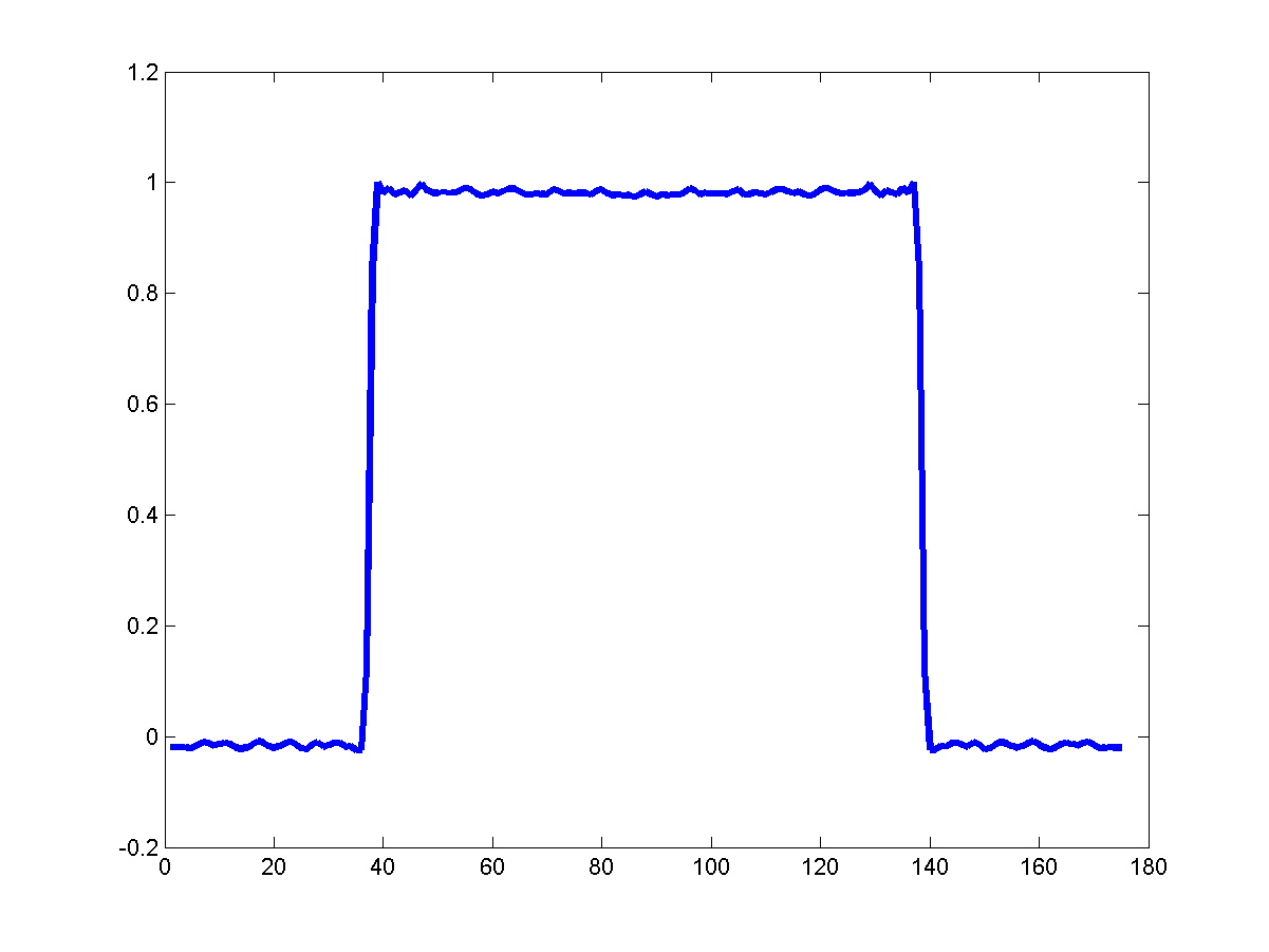
u(x,y)={1, if x2+y2r0, otherwise𝑢𝑥𝑦cases1 if superscript𝑥2superscript𝑦2𝑟0 otherwise\displaystyle u(x,y)=\begin{cases}1,&\mbox{ if }x^{2}+y^{2}\leq r\\ 0,&\mbox{ otherwise}\end{cases} (2.28)
g(θ,s)=θu(s)={2r2s2, for |s|<r0, otherwise𝑔𝜃𝑠subscript𝜃𝑢𝑠cases2superscript𝑟2superscript𝑠2 for 𝑠𝑟0 otherwise\displaystyle g(\theta,s)=\mathcal{R}_{\theta}u(s)=\begin{cases}2\sqrt{r^{2}-s^{2}},&\mbox{ for }|s|<r\\ 0,&\mbox{ otherwise}\end{cases} (2.29)

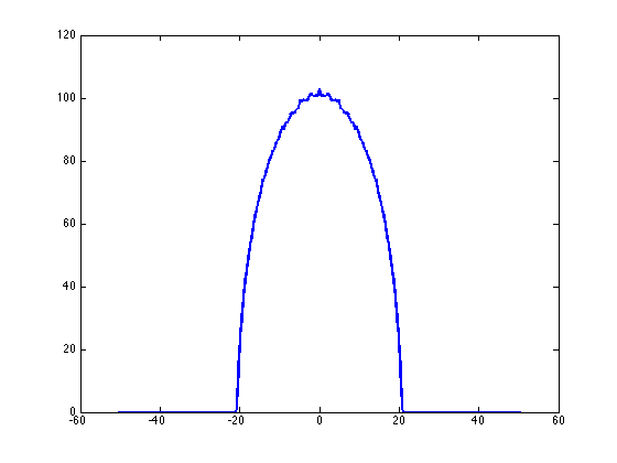
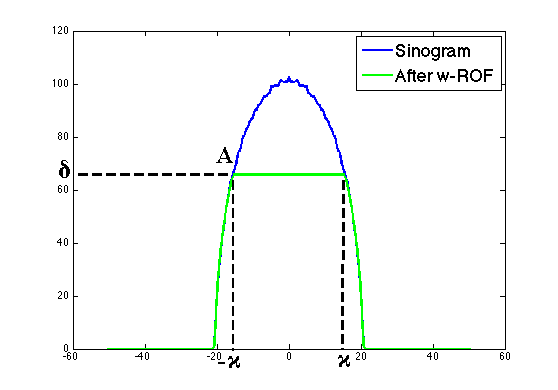
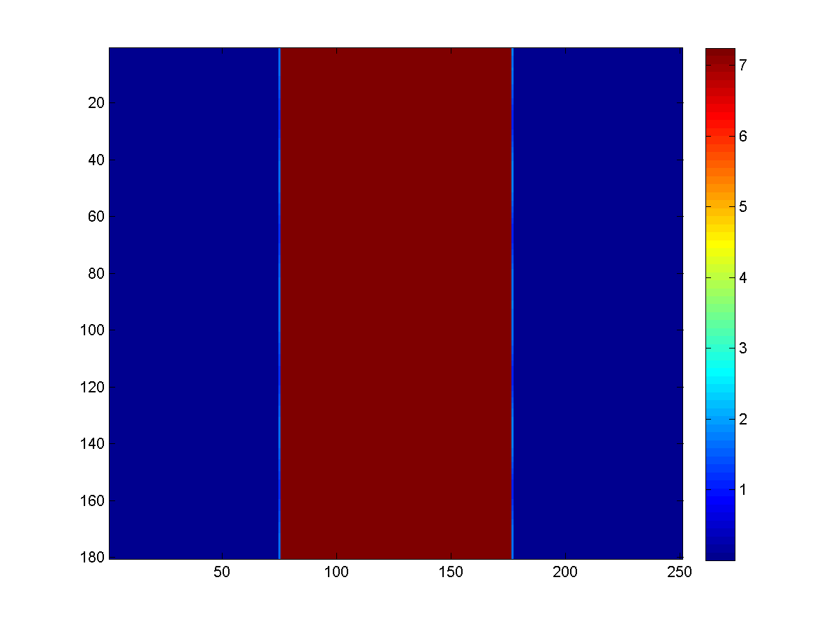
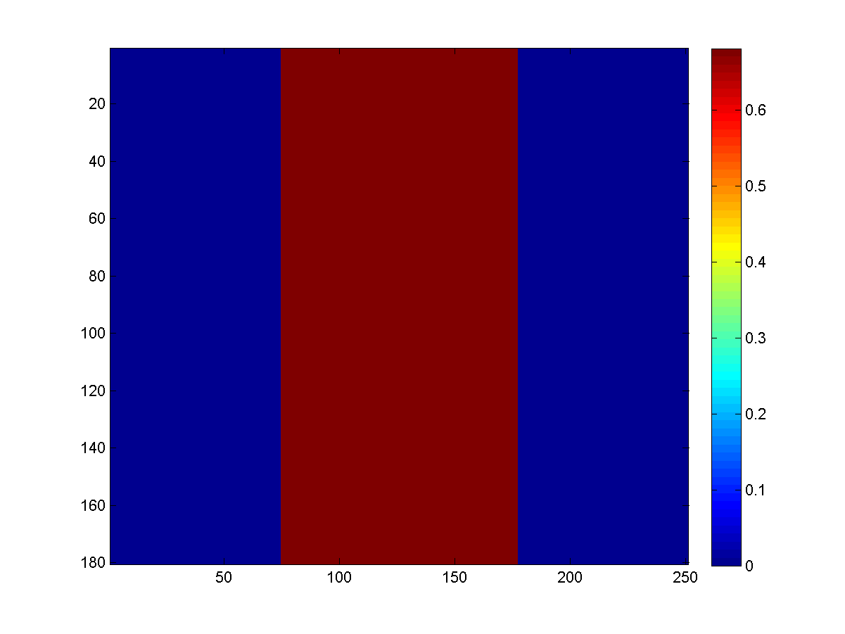
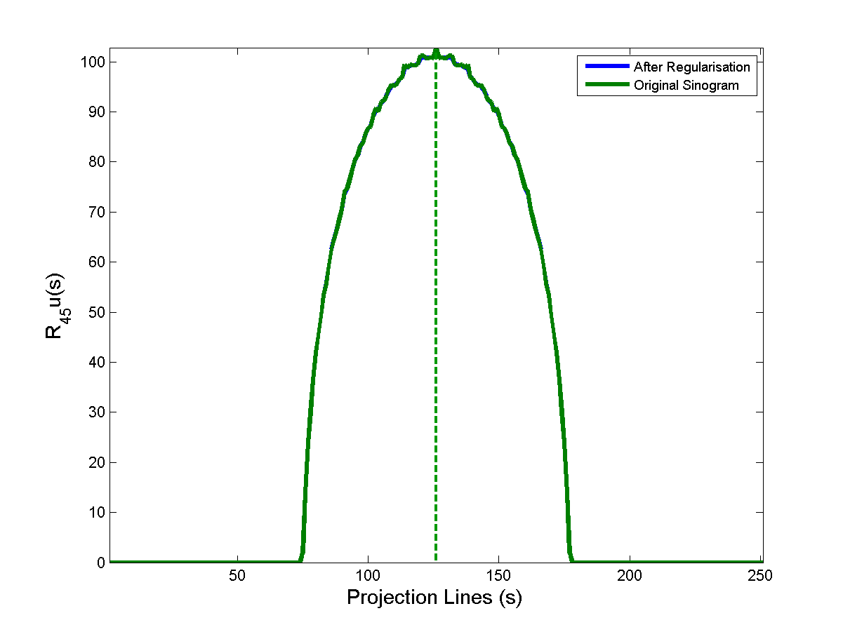
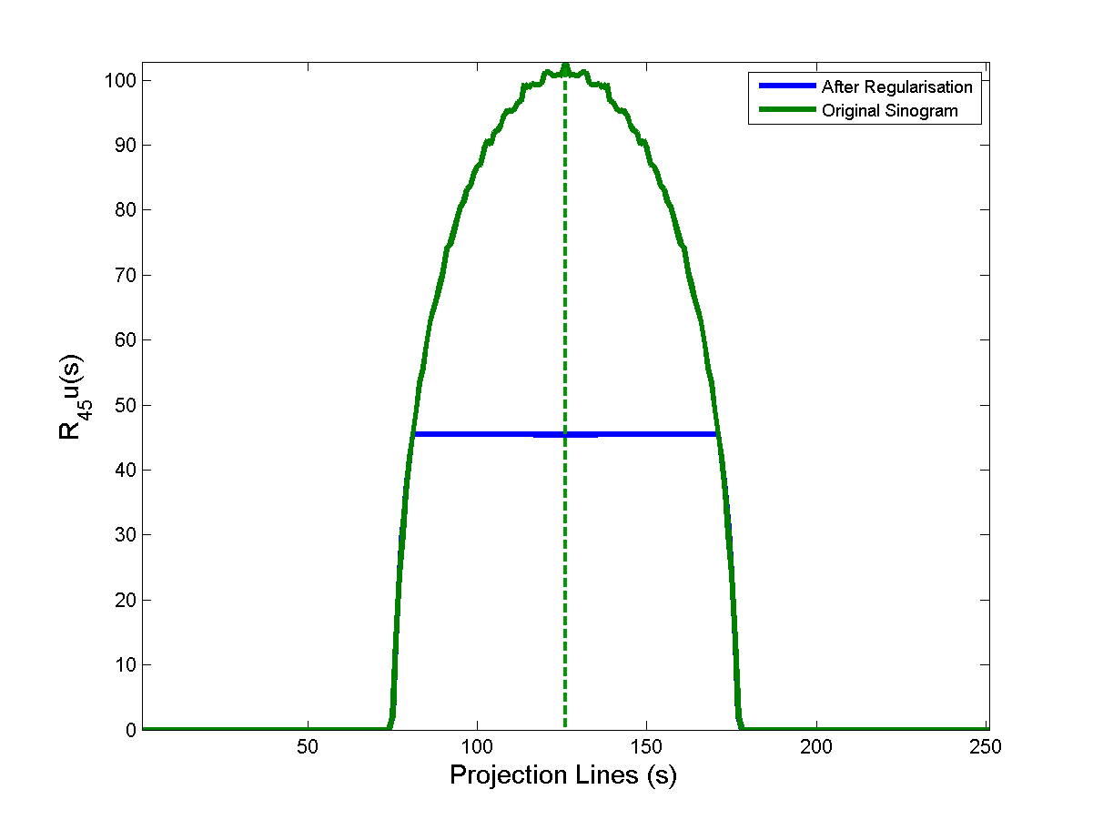
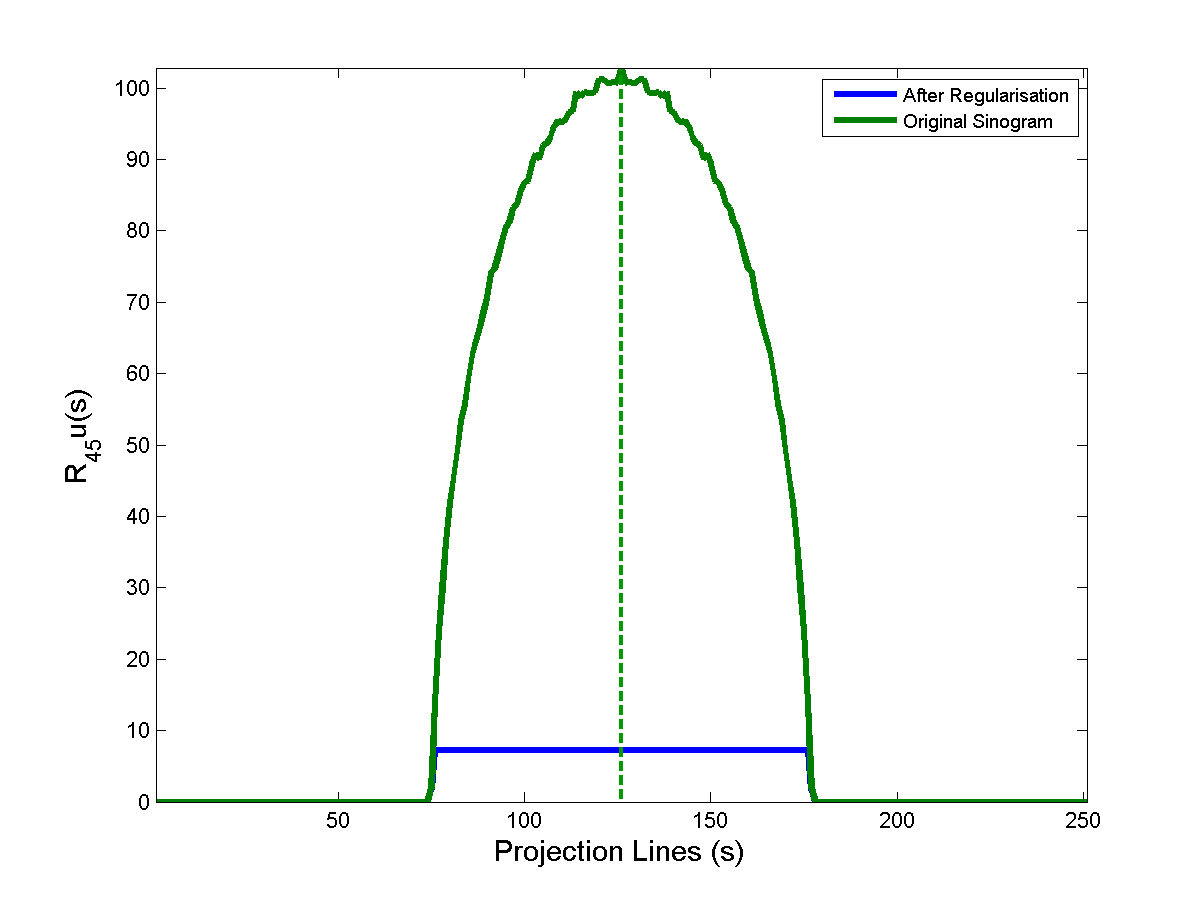
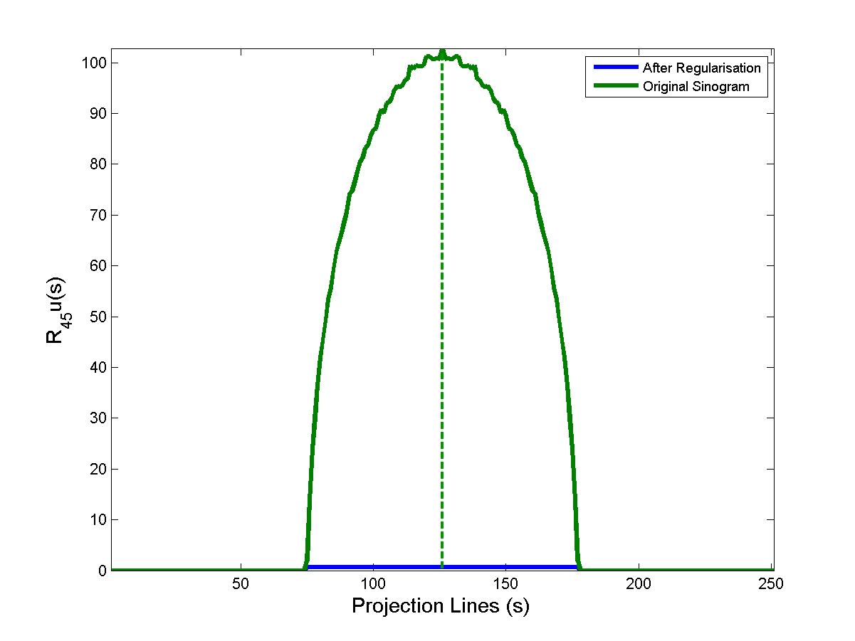
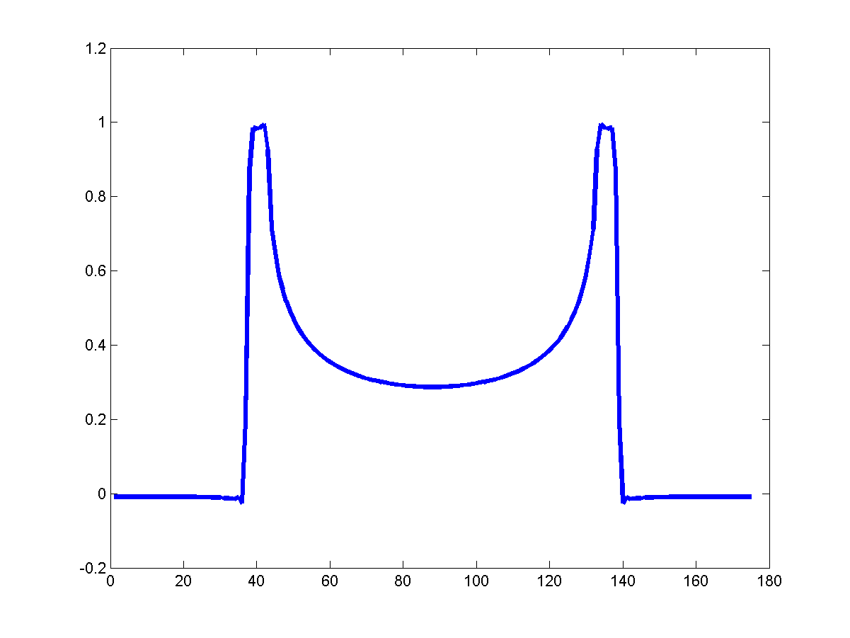
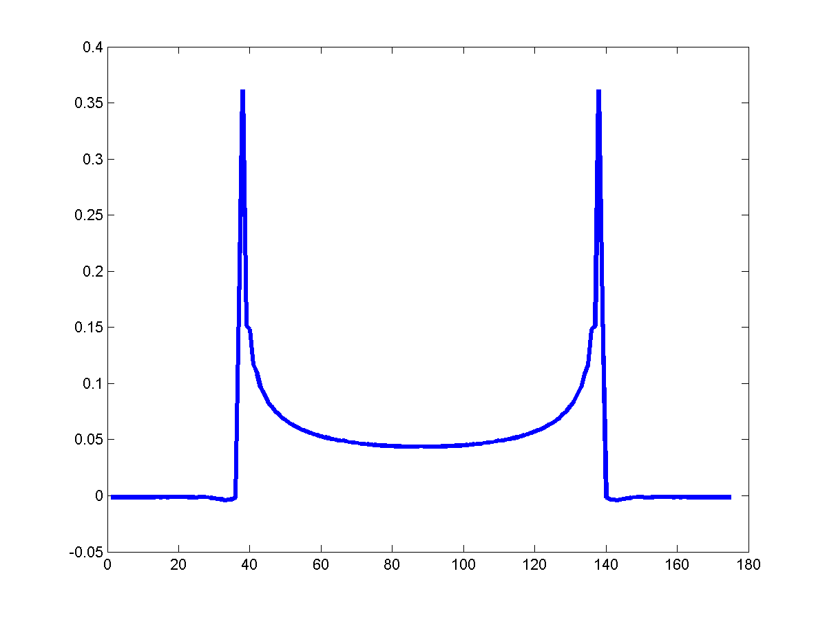
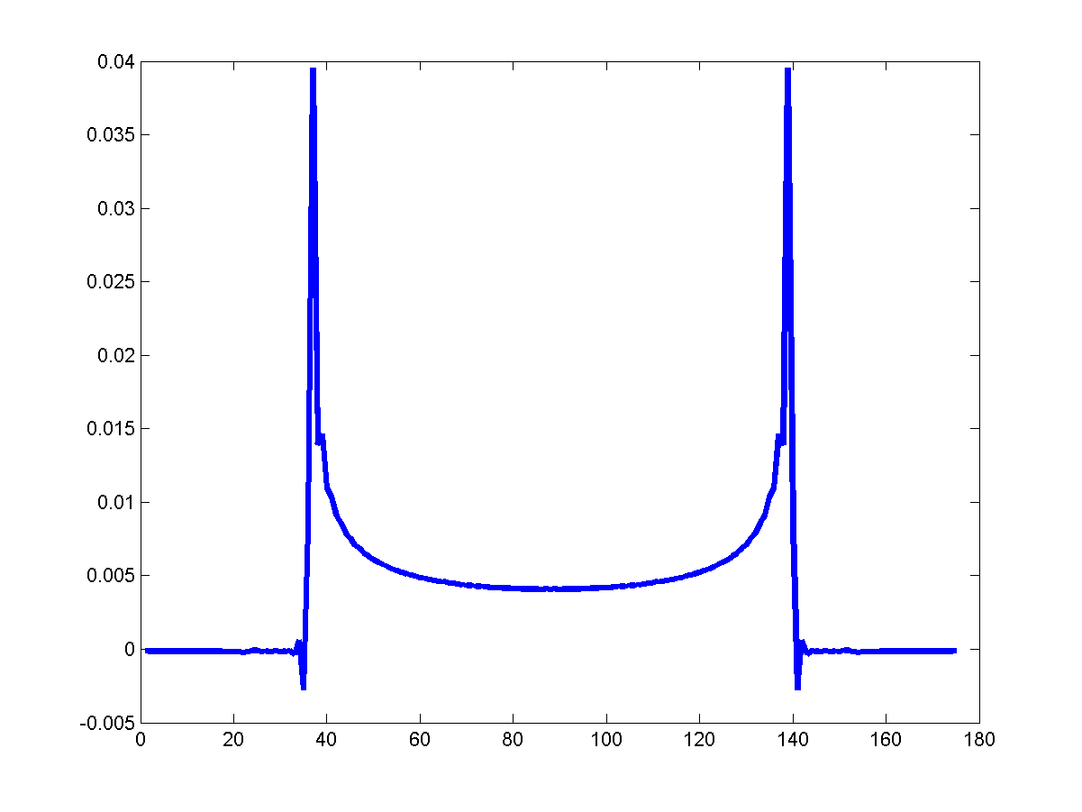
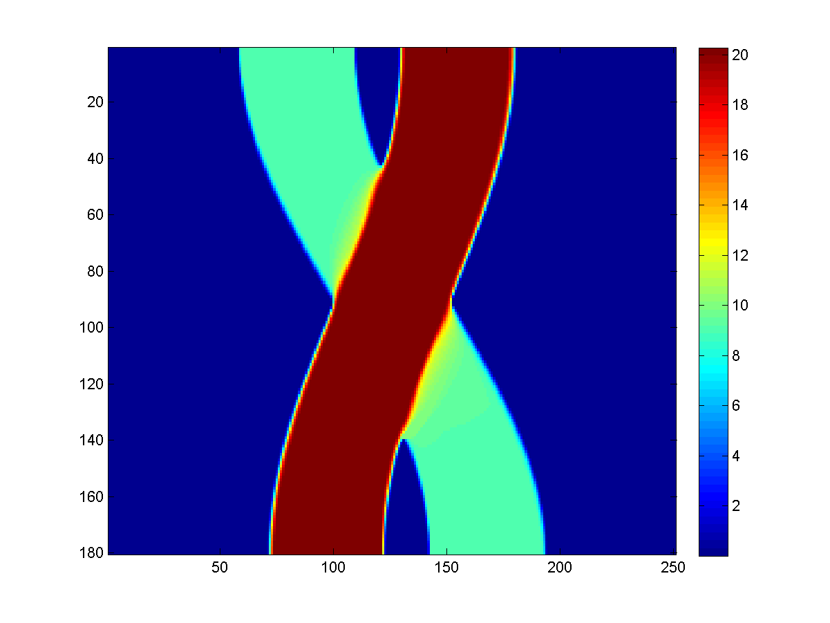
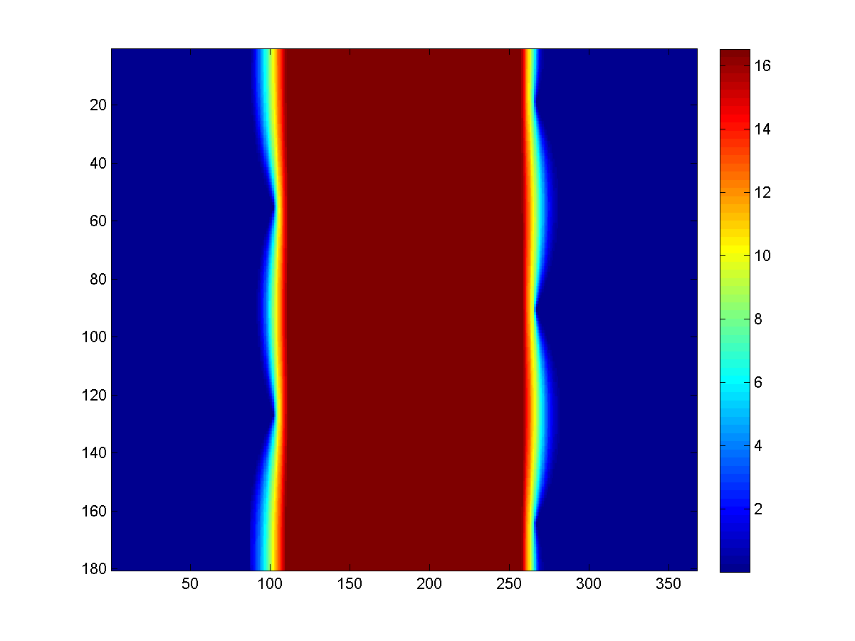
In Figure (2(b)), the given sinogram g𝑔g and the corresponding regularised solution v𝑣v of (2.27) for β=10𝛽10\beta=10 is shown. We make the following Ansatz for a solution of (2.27)

v(s)={δ=g(κ), for |s|κ,g(s), for κ<|s|<r,0, otherwise.𝑣𝑠cases𝛿𝑔𝜅 for 𝑠𝜅𝑔𝑠 for 𝜅𝑠𝑟0 otherwise.v(s)=\begin{cases}\delta=g(\kappa),&\mbox{ for }|s|\leq\kappa,\\ g(s),&\mbox{ for }\kappa<|s|<r,\\ 0,&\mbox{ otherwise.}\end{cases} (2.30)
Refer to caption
(a) Given sinogram g𝑔g
Refer to caption
(b) TV regularised sinogram v𝑣v
Fig. 2: The original sinogram g𝑔g with r=50.5𝑟50.5r=50.5, plotted at 454545 degrees in (a) and the regularised sinogram v𝑣v with β=10𝛽10\beta=10 in (b).

Note that, since gC(r,r)𝑔𝐶𝑟𝑟g\in C(-r,r), a solution v𝑣v of (2.27) is in C(r,r)𝐶𝑟𝑟C(-r,r) and hence also in W1,1(r,r)superscript𝑊11𝑟𝑟W^{1,1}(-r,r) [13]. Therefore, |Dv|(Σ)=Σ|v|𝑑x𝐷𝑣ΣsubscriptΣ𝑣differential-d𝑥|Dv|(\Sigma)=\int_{\Sigma}|\nabla v|~{}dx. Then, if we plug-in (2.30) in (2.27), we obtain

argminv0 a.e {βv1+12Σ(gv)2g}subscriptargmin𝑣0 a.e 𝛽subscriptdelimited-∥∥𝑣112subscriptΣsuperscript𝑔𝑣2𝑔\displaystyle\operatorname*{arg\,min}_{v\geq 0\mbox{ a.e }}\left\{\beta\left\lVert\nabla v\right\rVert_{1}+\frac{1}{2}\int_{\Sigma}\frac{(g-v)^{2}}{g}\right\}
=argminv0 a.e {4βr2κ2+0κ(2r2s2+v22r2s22v)𝑑s}absentsubscriptargmin𝑣0 a.e 4𝛽superscript𝑟2superscript𝜅2superscriptsubscript0𝜅2superscript𝑟2superscript𝑠2superscript𝑣22superscript𝑟2superscript𝑠22𝑣differential-d𝑠\displaystyle=\operatorname*{arg\,min}_{v\geq 0\mbox{ a.e }}\left\{4\beta\sqrt{r^{2}-\kappa^{2}}+\int_{0}^{\kappa}\left(2\sqrt{r^{2}-s^{2}}+\frac{v^{2}}{2\sqrt{r^{2}-s^{2}}}-2v\right)ds\right\}

which can be simplified to

argminκ{(4β3κ)r2κ2+(3r22κ2)arcsin(κr)}subscriptargmin𝜅4𝛽3𝜅superscript𝑟2superscript𝜅23superscript𝑟22superscript𝜅2arcsin𝜅𝑟\operatorname*{arg\,min}_{\kappa}\left\{(4\beta-3\kappa)\sqrt{r^{2}-\kappa^{2}}+(3r^{2}-2\kappa^{2})\mathrm{arcsin}(\frac{\kappa}{r})\right\} (2.31)

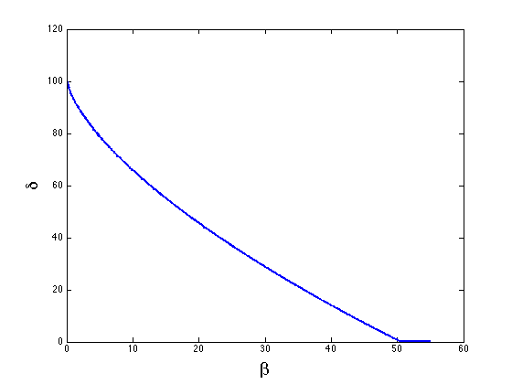
Numerically solving (2.31) under the constraint 0<|κ|<r0𝜅𝑟0<|\kappa|<r, we obtain a value for κ𝜅\kappa that we can substitute in (2.30) and find the corresponding value of our solution after the regularisation. We solve (2.31) with MATLAB’s built-in routine fminbnd in κ[0,r)𝜅0𝑟\kappa\in[0,r). In Figure 3, we present how the β𝛽\beta parameter relates to the constant height value δ𝛿\delta of the computed regularised solution. Clearly, for small values of β𝛽\beta, there is no significant effect of the total variation regularisation but as we increase β𝛽\beta we have that δ𝛿\delta decreases to zero, while κ𝜅\kappa tends to r𝑟r.

Refer to caption
Fig. 3: The relation between the regularisation parameter β𝛽\beta and δ𝛿\delta in (2.30), computed using (2.31) for the example in Figure 2. The parameter β𝛽\beta varies from 0.0010.0010.001 to 555555 with step size 0.10.10.1.

Before we apply the inverse Radon transform on (2.30) and find the corresponding solution in the image space, we need to verify its optimality. The following theorem ensures that the candidate solution (2.30) for the problem (2.27) is indeed optimal.

Theorem 2.5.

The unique solution of the minimisation problem (2.27) is defined by (2.30).

Proof.

The optimality condition on (2.27) implies that:

0J(u)βq+vgg=0q|Du|(Ω)0𝐽𝑢𝛽𝑞𝑣𝑔𝑔0𝑞𝐷𝑢Ω0\in\partial J(u)\Leftrightarrow\beta q+\frac{v-g}{\sqrt{g}}=0\mbox{, }q\in\partial|Du|(\Omega) (2.32)

We can characterise the subdifferential of total variation, see [7], as

|Du|(Σ)={divp:pCo(Σ),p1,divp,v=|Du|(Σ)}𝐷𝑢Σconditional-setdiv𝑝formulae-sequence𝑝subscriptsuperscript𝐶𝑜Σformulae-sequencesubscriptdelimited-∥∥𝑝1div𝑝𝑣𝐷𝑢Σ\partial|Du|(\Sigma)=\left\{{\rm div}p:p\in C^{\infty}_{o}(\Sigma),\left\lVert p\right\rVert_{\infty}\leq 1,\left\langle{\rm div}p,v\right\rangle=|Du|(\Sigma)\right\} (2.33)

Therefore, in our case (2.32) becomes

βp(s)+v(s)g(s)g(s)=0, in sΣ𝛽superscript𝑝𝑠𝑣𝑠𝑔𝑠𝑔𝑠0, in 𝑠Σ\beta p^{\prime}(s)+\frac{v(s)-g(s)}{\sqrt{g(s)}}=0\mbox{, in }s\in\Sigma (2.34)

with 1p(s)11𝑝𝑠1-1\leq p(s)\leq 1 and Σp(s)v(s)=Σ|v(s)|subscriptΣsuperscript𝑝𝑠𝑣𝑠subscriptΣsuperscript𝑣𝑠\int_{\Sigma}p^{\prime}(s)v(s)=\int_{\Sigma}|v^{\prime}(s)|. If v is either increasing or decreasing on an interval IΣ𝐼ΣI\subset\Sigma, then through integration by parts one obtains p(s)v(s)=|v(s)|𝑝𝑠superscript𝑣𝑠superscript𝑣𝑠p(s)v^{\prime}(s)=|v^{\prime}(s)| which immediately implies that p=0superscript𝑝0p^{\prime}=0 and v=g𝑣𝑔v=g on I. However, when vg𝑣𝑔v\neq g on an interval IΣsuperscript𝐼ΣI^{\prime}\subset\Sigma, then p0superscript𝑝0p^{\prime}\neq 0 which is true only if v(s)=0superscript𝑣𝑠0v^{\prime}(s)=0 on Isuperscript𝐼I^{\prime}, i.e., v is constant.

For computing the regularised image that corresponds to a solution of (2.27) we first note that the rotational symmetry of the object in image space allows to simplify the Radon transform and its inverse. In this case the Radon transform coincides with the so-called Abel transform, cf. [26, Chapter 8]. More precisely, if u𝑢u is a radial function and u(x,y)=f(x2+y2)𝑢𝑥𝑦𝑓superscript𝑥2superscript𝑦2u(x,y)=f(\sqrt{x^{2}+y^{2}}) we have

θu(s)=2sf(r)rr2s2𝑑rsubscript𝜃𝑢𝑠2superscriptsubscript𝑠𝑓𝑟𝑟superscript𝑟2superscript𝑠2differential-d𝑟\mathcal{R}_{\theta}u(s)=2\int_{s}^{\infty}\frac{f(r)r}{\sqrt{r^{2}-s^{2}}}dr (2.35)

Using (2.35), we can recover analytically the solution u𝑢u for a regularised sinogram (2.30). The Abel transform and the inverse Abel transform in this case are

𝒜(u(r~))(x)𝒜𝑢~𝑟𝑥\displaystyle\mathcal{A}(u(\widetilde{r}))(x) =2xr~u(r~)r~2x2𝑑r~absent2superscriptsubscript𝑥~𝑟𝑢~𝑟superscript~𝑟2superscript𝑥2differential-d~𝑟\displaystyle=2\int_{x}^{\infty}\frac{\widetilde{r}u(\widetilde{r})}{\sqrt{\widetilde{r}^{2}-x^{2}}}d\widetilde{r} (2.36)
u(r~)𝑢~𝑟\displaystyle u(\widetilde{r}) =1r~πddr~r~r𝒜(u(r~))(x)x2r2𝑑xabsent1~𝑟𝜋𝑑𝑑~𝑟superscriptsubscript~𝑟𝑟𝒜𝑢~𝑟𝑥superscript𝑥2superscript𝑟2differential-d𝑥\displaystyle=-\frac{1}{\widetilde{r}\pi}\frac{d}{d\widetilde{r}}\int_{\widetilde{r}}^{\infty}\frac{r\mathcal{A}(u(\widetilde{r}))(x)}{\sqrt{x^{2}-r^{2}}}dx (2.37)
Refer to caption
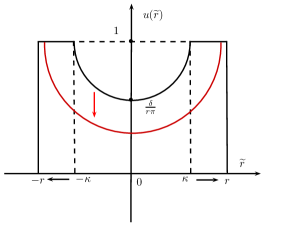
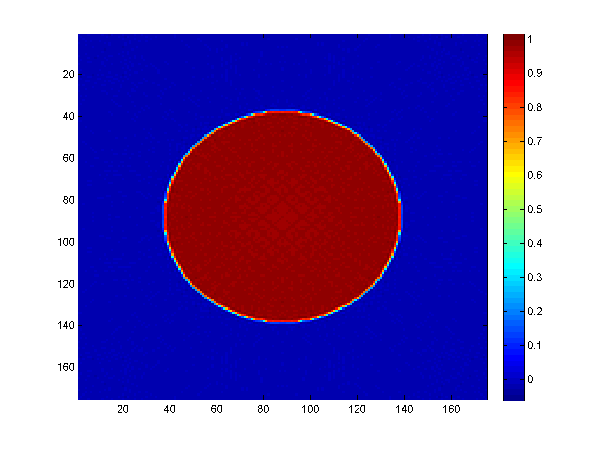
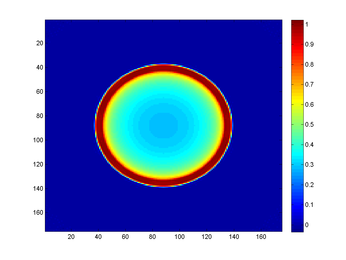
Fig. 4: The solution u(r~)𝑢~𝑟u(\widetilde{r}) (solid line) given in (2.38) inside the interval [r,r]𝑟𝑟[-r,r] and zero outside. The black and the red curve constitute the regularised solution for a smaller and larger value of β𝛽\beta, respectively. The larger β𝛽\beta the more the solution concentrates around the boundaries of the disc.

Setting u(r~)=1𝑢~𝑟1u(\widetilde{r})=1 and replacing the upper limit of the integral \infty by r𝑟r in (2.36), the expression in (2.36) matches the expression for the Radon transform in (2.29). Therefore, we plug-in (2.30) in (2.37) and focus on the constant part of the sinogram for κr~κ𝜅~𝑟𝜅-\kappa\leq\widetilde{r}\leq\kappa,

u(r~)𝑢~𝑟\displaystyle u(\widetilde{r}) =1r~πddr~r~rxδx2r~2𝑑x=δπr2r~2absent1~𝑟𝜋𝑑𝑑~𝑟superscriptsubscript~𝑟𝑟𝑥𝛿superscript𝑥2superscript~𝑟2differential-d𝑥𝛿𝜋superscript𝑟2superscript~𝑟2\displaystyle=-\frac{1}{\widetilde{r}\pi}\frac{d}{d\widetilde{r}}\int_{\widetilde{r}}^{r}\frac{x\delta}{\sqrt{x^{2}-\widetilde{r}^{2}}}dx=\frac{\delta}{\pi\sqrt{r^{2}-\widetilde{r}^{2}}} (2.38)

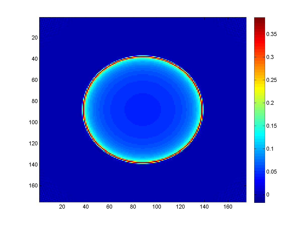
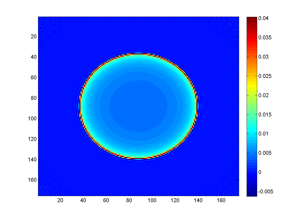
We observe that the reconstructed image is affected by the initial loss of contrast δ𝛿\delta of the sinogram regularisation in (2.30) and depends radially on r~~𝑟\widetilde{r}. In Figure 4, we present the regularised solution u𝑢u for two values of β𝛽\beta. Recall, as we increase β𝛽\beta (red curve), we have that δ0𝛿0\delta\rightarrow 0 and κr𝜅𝑟\kappa\rightarrow r.

3 Numerical Implementation

In this section we discuss the numerical solution of the minimisation problem (2.1). We employ the split Bregman technique [19] which separates the problem into two subproblems – one in image space and one in projection space – that are solved iteratively in an alternating fashion. In order to present the numerical solution we start with formulating (2.1) in a discrete setting.

3.1 Discrete Setting

Let (ui,j)subscript𝑢𝑖𝑗(u_{i,j}), i=1,,m𝑖1𝑚i=1,\ldots,m, j=1,,n𝑗1𝑛j=1,\ldots,n be the discretised image defined on a rectangular grid of size m×n𝑚𝑛m\times n, m,n>0𝑚𝑛0m,n>0, and (vi,j)subscript𝑣𝑖𝑗(v_{i,j}), i=1,,k𝑖1𝑘i=1,\ldots,k, j=1,,l𝑗1𝑙j=1,\ldots,l the discretisation for an element in the sinogram space Σ=[0,π)×[r,r]Σ0𝜋𝑟𝑟\Sigma=[0,\pi)\times[-r,r] where k denotes the number of lines and l the number of angles. The values ui,jsubscript𝑢𝑖𝑗u_{i,j} and vi,jsubscript𝑣𝑖𝑗v_{i,j} are defined on two-dimensional grids. They are rearranged into one-dimensional vectors unm𝑢superscript𝑛𝑚u\in\mathbb{R}^{nm} and vkl𝑣superscript𝑘𝑙v\in\mathbb{R}^{kl} by appending the columns of the array to each other, starting from the leftmost. Then, the discrete gradient for um×n𝑢superscript𝑚𝑛u\in\mathbb{R}^{m\times n} is a matrix 2nm×nmsuperscript2𝑛𝑚𝑛𝑚\nabla\in\mathbb{R}^{2nm\times nm} which is the standard forward difference approximation of the gradient in the continuum. More precisely, applying the discrete gradient to u𝑢u gives u=((u)1,(u)2)2nm𝑢subscript𝑢1subscript𝑢2superscript2𝑛𝑚\nabla u=((\nabla u)_{1},(\nabla u)_{2})\in\mathbb{R}^{2nm} with

(u)1(i,j)subscript𝑢1𝑖𝑗\displaystyle(\nabla u)_{1}(i,j) ={u(i,j+1)u(i,j), if 1in,1j<m,0, if 1in,j=m.absentcases𝑢𝑖𝑗1𝑢𝑖𝑗formulae-sequence if 1𝑖𝑛1𝑗𝑚0formulae-sequence if 1𝑖𝑛𝑗𝑚\displaystyle=\begin{cases}u(i,j+1)-u(i,j),&\mbox{ if }1\leq i\leq n,1\leq j<m,\\ 0,&\mbox{ if }1\leq i\leq n,j=m.\end{cases}
(u)2(i,j)subscript𝑢2𝑖𝑗\displaystyle(\nabla u)_{2}(i,j) ={u(i+1,j)u(i,j), if 1i<n,1jm,0, if i=n,1jm.absentcases𝑢𝑖1𝑗𝑢𝑖𝑗formulae-sequence if 1𝑖𝑛1𝑗𝑚0formulae-sequence if 𝑖𝑛1𝑗𝑚\displaystyle=\begin{cases}u(i+1,j)-u(i,j),&\mbox{ if }1\leq i<n,1\leq j\leq m,\\ 0,&\mbox{ if }i=n,1\leq j\leq m.\end{cases}

The discrete divergence is defined as its adjoint, cf. [14], and is given by

div:2nmnm:divsuperscript2𝑛𝑚superscript𝑛𝑚\displaystyle{\rm div}:\mathbb{R}^{2nm}\rightarrow\mathbb{R}^{nm} with div(z)u=zuwith div𝑧𝑢𝑧𝑢\displaystyle\mbox{ with }{\rm div}(z)\cdot u=-z\cdot\nabla u

Further, to approximate the Radon transform \mathcal{R} we introduce the discrete Radon transform as a mapping R:nmkl:𝑅superscript𝑛𝑚superscript𝑘𝑙R:\mathbb{R}^{nm}\rightarrow\mathbb{R}^{kl} and its inverse R1:klnm:superscript𝑅1superscript𝑘𝑙superscript𝑛𝑚R^{-1}:\mathbb{R}^{kl}\rightarrow\mathbb{R}^{nm}. In the numerical implementation the discrete Radon transform is represented by a sparse matrix Rkl×nm𝑅superscript𝑘𝑙𝑛𝑚R\in\mathbb{R}^{kl\times nm} which acts on unm𝑢superscript𝑛𝑚u\in\mathbb{R}^{nm} to obtain a sinogram image vkl𝑣superscript𝑘𝑙v\in\mathbb{R}^{kl}. Defining x(θi^,sj^)𝑥subscript𝜃^𝑖subscript𝑠^𝑗x(\theta_{\hat{i}},s_{\hat{j}}), i^=1,,k^𝑖1𝑘\hat{i}=1,\ldots,k, j^=1,,l^𝑗1𝑙\hat{j}=1,\ldots,l, the line defined by θi^,sj^subscript𝜃^𝑖subscript𝑠^𝑗\theta_{\hat{i}},s_{\hat{j}}, we can define for i=1,,m𝑖1𝑚i=1,\ldots,m and j=1,,n𝑗1𝑛j=1,\ldots,n

ψi,j(θi^,sj^)={1, where the line x(θi^,sj^) goes through the pixel (i,j)0, otherwise.subscript𝜓𝑖𝑗subscript𝜃^𝑖subscript𝑠^𝑗cases1, where the line 𝑥subscript𝜃^𝑖subscript𝑠^𝑗 goes through the pixel 𝑖𝑗0, otherwise.\psi_{i,j}(\theta_{\hat{i}},s_{\hat{j}})=\begin{cases}1&\mbox{, where the line }x(\theta_{\hat{i}},s_{\hat{j}})\mbox{ goes through the pixel }(i,j)\\ 0&\mbox{, otherwise.}\end{cases} (3.1)

Using this notation and the linearity of the Radon transform, we define the discrete Radon transform as

Ru(θi^,sj^)=i=1mj=1nui,jψi,j(θi^,sj^)𝑅𝑢subscript𝜃^𝑖subscript𝑠^𝑗superscriptsubscript𝑖1𝑚superscriptsubscript𝑗1𝑛subscript𝑢𝑖𝑗subscript𝜓𝑖𝑗subscript𝜃^𝑖subscript𝑠^𝑗Ru(\theta_{\hat{i}},s_{\hat{j}})=\sum_{i=1}^{m}\sum_{j=1}^{n}u_{i,j}\mathcal{R}\psi_{i,j}(\theta_{\hat{i}},s_{\hat{j}}) (3.2)

where ψi,j(θi^,sj^)subscript𝜓𝑖𝑗subscript𝜃^𝑖subscript𝑠^𝑗\mathcal{R}\psi_{i,j}(\theta_{\hat{i}},s_{\hat{j}}) is equal to the length of the intersection of the projection line with the pixel (i,j)𝑖𝑗(i,j).

With these discrete quantities we define the discrete functional F𝐹F by

F(u)=au1+β(Ru)1+12k,l(gu)2g,𝐹𝑢𝑎subscriptdelimited-∥∥𝑢1𝛽subscriptdelimited-∥∥𝑅𝑢112subscript𝑘𝑙superscript𝑔𝑢2𝑔F(u)=a\left\lVert\nabla u\right\rVert_{1}+\beta\left\lVert(\nabla Ru)\right\rVert_{1}+\frac{1}{2}\sum_{k,l}\frac{(g-\mathcal{R}u)^{2}}{g}, (3.3)

and the discrete version of the minimisation problem (2.1)

minum×nF(u).subscript𝑢superscript𝑚𝑛𝐹𝑢\min_{u\in\mathbb{R}^{m\times n}}F(u). (3.4)

3.2 Split Bregman Algorithm

To solve the problems defined in (3.3) we employ the Bregman iteration [25] combined with a splitting technique. The resulting algorithm is called Split Bregman method which is proposed in [19] to efficiently solve total variation and 1subscript1\ell_{1} regularised image processing problems. The idea of this splitting procedure is to replace a complex and costly minimisation problem by a sequence of simple and cheaply to solve minimisation problems and to set up an iteration in which they are solved alternatingly. Note, that the Split Bregman method can be equivalently phrased in terms of an augmented Lagrange method and Douglas-Rachford splitting, cf. [32, 17, 33]. We follow [19] to adapt the Split Bregman algorithm to the solution of (2.1). To do so, we consider

min{u:u0 a.e.}αu1+β(Ru)1+12k,l(gRu)2g.subscriptconditional-set𝑢𝑢0 a.e.𝛼subscriptdelimited-∥∥𝑢1𝛽subscriptdelimited-∥∥𝑅𝑢112subscript𝑘𝑙superscript𝑔𝑅𝑢2𝑔\min_{\{u:\ u\geq 0\mbox{ a.e.}\}}\alpha\left\lVert\nabla u\right\rVert_{1}+\beta\left\lVert\nabla(Ru)\right\rVert_{1}+\frac{1}{2}\sum_{k,l}\frac{(g-Ru)^{2}}{g}. (3.5)

We start with replacing (3.5) by an equivalent constrained minimisation problem for two unknowns, the image um×n𝑢superscript𝑚𝑛u\in\mathbb{R}^{m\times n} and the sinogram vk×l𝑣superscript𝑘𝑙v\in\mathbb{R}^{k\times l}, related to each other by v=Ru𝑣𝑅𝑢v=Ru. This gives

min{(u,v):u0 a.e.}αu1+βv1+12k,l(gv)2g s.t v=Ru.subscriptconditional-set𝑢𝑣𝑢0 a.e.𝛼subscriptdelimited-∥∥𝑢1𝛽subscriptdelimited-∥∥𝑣112subscript𝑘𝑙superscript𝑔𝑣2𝑔 s.t 𝑣𝑅𝑢\min_{\{(u,v):\ u\geq 0\mbox{ a.e.}\}}\alpha\left\lVert\nabla u\right\rVert_{1}+\beta\left\lVert\nabla v\right\rVert_{1}+\frac{1}{2}\sum_{k,l}\frac{(g-v)^{2}}{g}\mbox{ s.t }v=Ru. (3.6)

For computational efficiency reasons, we introduce three additional variables

z=u,w=v and u=u~formulae-sequence𝑧𝑢𝑤𝑣 and 𝑢~𝑢z=\nabla u,w=\nabla v\mbox{ and }u=\widetilde{u} (3.7)

and rephrase (3.6) again into

min{(u,u~,v,z,w):u~0 a.e.,satisfying (3.7)}αz1+βw1+12k,l(gv)2gsubscriptconditional-set𝑢~𝑢𝑣𝑧𝑤~𝑢0 a.e.satisfying (3.7)𝛼subscriptdelimited-∥∥𝑧1𝛽subscriptdelimited-∥∥𝑤112subscript𝑘𝑙superscript𝑔𝑣2𝑔\min_{\{(u,\widetilde{u},v,z,w):\ \widetilde{u}\geq 0\mbox{ a.e.},~{}\mbox{satisfying \eqref{constraints}}\}}\alpha\left\lVert z\right\rVert_{1}+\beta\left\lVert w\right\rVert_{1}+\frac{1}{2}\sum_{k,l}\frac{(g-v)^{2}}{g} (3.8)

Then, we could iteratively solve the constrained minimisation problem (3.8) by Bregman iteration. Starting with initial conditions b10k×l,b20(k×l)2,b30(m×n)2,b40(m×n)formulae-sequencesuperscriptsubscript𝑏10superscript𝑘𝑙formulae-sequencesuperscriptsubscript𝑏20superscriptsuperscript𝑘𝑙2formulae-sequencesuperscriptsubscript𝑏30superscriptsuperscript𝑚𝑛2superscriptsubscript𝑏40superscript𝑚𝑛b_{1}^{0}\in\mathbb{R}^{k\times l},b_{2}^{0}\in(\mathbb{R}^{k\times l})^{2},b_{3}^{0}\in(\mathbb{R}^{m\times n})^{2},b_{4}^{0}\in(\mathbb{R}^{m\times n}) we iteratively solve for k=0,1,𝑘01k=0,1,\ldots

argminu,u~,v,z,wsubscriptargmin𝑢~𝑢𝑣𝑧𝑤\displaystyle\operatorname*{arg\,min}_{u,\widetilde{u},v,z,w} {αz1+βw1+(gv)2g+ι(u~>0)+λ12b1k+uv22+λ22b2k+vw22\displaystyle\bigg{\{}\alpha\left\lVert z\right\rVert_{1}+\beta\left\lVert w\right\rVert_{1}+\sum\frac{(g-v)^{2}}{g}+\iota_{(\widetilde{u}>0)}+\frac{\lambda_{1}}{2}\left\lVert b_{1}^{k}+\mathcal{R}u-v\right\rVert_{2}^{2}+\frac{\lambda_{2}}{2}\left\lVert b_{2}^{k}+\nabla v-w\right\rVert_{2}^{2}
+λ32b3k+uz22+λ42b4k+uu~22}\displaystyle+\frac{\lambda_{3}}{2}\left\lVert b_{3}^{k}+\nabla u-z\right\rVert_{2}^{2}+\frac{\lambda_{4}}{2}\left\lVert b_{4}^{k}+u-\widetilde{u}\right\rVert_{2}^{2}\bigg{\}}
b1k+1superscriptsubscript𝑏1𝑘1\displaystyle b_{1}^{k+1} =b1k+uk+1vk+1b2k+1=b2k+vk+1wk+1formulae-sequenceabsentsuperscriptsubscript𝑏1𝑘superscript𝑢𝑘1superscript𝑣𝑘1superscriptsubscript𝑏2𝑘1superscriptsubscript𝑏2𝑘superscript𝑣𝑘1superscript𝑤𝑘1\displaystyle=b_{1}^{k}+\mathcal{R}u^{k+1}-v^{k+1}\qquad b_{2}^{k+1}=b_{2}^{k}+\nabla v^{k+1}-w^{k+1}
b3k+1superscriptsubscript𝑏3𝑘1\displaystyle b_{3}^{k+1} =b3k+uk+1zk+1b4k+1=b4k+uk+1u~k+1,formulae-sequenceabsentsuperscriptsubscript𝑏3𝑘superscript𝑢𝑘1superscript𝑧𝑘1superscriptsubscript𝑏4𝑘1superscriptsubscript𝑏4𝑘superscript𝑢𝑘1superscript~𝑢𝑘1\displaystyle=b_{3}^{k}+\nabla u^{k+1}-z^{k+1}\qquad b_{4}^{k+1}=b_{4}^{k}+u^{k+1}-\widetilde{u}^{k+1},

with Lagrange multipliers (λi)i=14>0superscriptsubscriptsubscript𝜆𝑖𝑖140(\lambda_{i})_{i=1}^{4}>0, b1kk×lsuperscriptsubscript𝑏1𝑘superscript𝑘𝑙b_{1}^{k}\in\mathbb{R}^{k\times l}, b2k(k×l)2superscriptsubscript𝑏2𝑘superscriptsuperscript𝑘𝑙2b_{2}^{k}\in(\mathbb{R}^{k\times l})^{2}, b3k(m×n)2superscriptsubscript𝑏3𝑘superscriptsuperscript𝑚𝑛2b_{3}^{k}\in(\mathbb{R}^{m\times n})^{2} and b4k(m×n)superscriptsubscript𝑏4𝑘superscript𝑚𝑛b_{4}^{k}\in(\mathbb{R}^{m\times n}) and ι(u~>0)subscript𝜄~𝑢0\iota_{(\widetilde{u}>0)} being the characteristic function for the positivity constraint on u~~𝑢\widetilde{u}. To progress, in each iteration above we would need to solve a minimisation problem in all u,u~,v,z,w𝑢~𝑢𝑣𝑧𝑤u,\widetilde{u},v,z,w at the same time which is numerically very involved. Instead, we use the split Bregman idea of [19] and in each iteration solve a sequence of decoupled problems in u,u~,v,z,w𝑢~𝑢𝑣𝑧𝑤u,\widetilde{u},v,z,w, that is

vk+1superscript𝑣𝑘1\displaystyle v^{k+1} =argminv{12(gv)2g+λ12b1k+Rukv22\displaystyle=\operatorname*{arg\,min}_{v}\bigg{\{}\frac{1}{2}\sum\frac{(g-v)^{2}}{g}+\frac{\lambda_{1}}{2}\left\lVert b_{1}^{k}+Ru^{k}-v\right\rVert_{2}^{2}
+λ22b2k+vwk22}\displaystyle+\frac{\lambda_{2}}{2}\left\lVert b_{2}^{k}+\nabla v-w^{k}\right\rVert_{2}^{2}\bigg{\}} (3.9)
uk+1superscript𝑢𝑘1\displaystyle u^{k+1} =argminu{λ12b1k+Ruvk+122+λ32b3k+uzk22\displaystyle=\operatorname*{arg\,min}_{u}\bigg{\{}\frac{\lambda_{1}}{2}\left\lVert b_{1}^{k}+Ru-v^{k+1}\right\rVert_{2}^{2}+\frac{\lambda_{3}}{2}\left\lVert b_{3}^{k}+\nabla u-z^{k}\right\rVert_{2}^{2}
+λ42b4k+uu~k22}\displaystyle+\frac{\lambda_{4}}{2}\left\lVert b_{4}^{k}+u-\widetilde{u}^{k}\right\rVert_{2}^{2}\bigg{\}} (3.10)
u~k+1superscript~𝑢𝑘1\displaystyle\widetilde{u}^{k+1} =argminu~{ι(u~>0)+λ42b4k+uk+1u~22}absentsubscriptargmin~𝑢subscript𝜄~𝑢0subscript𝜆42superscriptsubscriptdelimited-∥∥superscriptsubscript𝑏4𝑘superscript𝑢𝑘1~𝑢22\displaystyle=\operatorname*{arg\,min}_{\widetilde{u}}\bigg{\{}\iota_{(\widetilde{u}>0)}+\frac{\lambda_{4}}{2}\left\lVert b_{4}^{k}+u^{k+1}-\widetilde{u}\right\rVert_{2}^{2}\bigg{\}} (3.11)
zk+1superscript𝑧𝑘1\displaystyle z^{k+1} =argminz{αz1+λ32b3k+uk+1z22}absentsubscriptargmin𝑧𝛼subscriptdelimited-∥∥𝑧1subscript𝜆32superscriptsubscriptdelimited-∥∥superscriptsubscript𝑏3𝑘superscript𝑢𝑘1𝑧22\displaystyle=\operatorname*{arg\,min}_{z}\bigg{\{}\alpha\left\lVert z\right\rVert_{1}+\frac{\lambda_{3}}{2}\left\lVert b_{3}^{k}+\nabla u^{k+1}-z\right\rVert_{2}^{2}\bigg{\}} (3.12)
wk+1superscript𝑤𝑘1\displaystyle w^{k+1} =argminw{βw1+λ22b2k+vk+1w22}absentsubscriptargmin𝑤𝛽subscriptdelimited-∥∥𝑤1subscript𝜆22superscriptsubscriptdelimited-∥∥superscriptsubscript𝑏2𝑘superscript𝑣𝑘1𝑤22\displaystyle=\operatorname*{arg\,min}_{w}\bigg{\{}\beta\left\lVert w\right\rVert_{1}+\frac{\lambda_{2}}{2}\left\lVert b_{2}^{k}+\nabla v^{k+1}-w\right\rVert_{2}^{2}\bigg{\}} (3.13)
b1k+1superscriptsubscript𝑏1𝑘1\displaystyle b_{1}^{k+1} =b1k+Ruk+1vk+1absentsuperscriptsubscript𝑏1𝑘𝑅superscript𝑢𝑘1superscript𝑣𝑘1\displaystyle=b_{1}^{k}+Ru^{k+1}-v^{k+1} (3.14)
b2k+1superscriptsubscript𝑏2𝑘1\displaystyle b_{2}^{k+1} =b2k+vk+1wk+1absentsuperscriptsubscript𝑏2𝑘superscript𝑣𝑘1superscript𝑤𝑘1\displaystyle=b_{2}^{k}+\nabla v^{k+1}-w^{k+1} (3.15)
b3k+1superscriptsubscript𝑏3𝑘1\displaystyle b_{3}^{k+1} =b3k+uk+1zk+1absentsuperscriptsubscript𝑏3𝑘superscript𝑢𝑘1superscript𝑧𝑘1\displaystyle=b_{3}^{k}+\nabla u^{k+1}-z^{k+1} (3.16)
b4k+1superscriptsubscript𝑏4𝑘1\displaystyle b_{4}^{k+1} =b4k+uk+1u~k+1absentsuperscriptsubscript𝑏4𝑘superscript𝑢𝑘1superscript~𝑢𝑘1\displaystyle=b_{4}^{k}+u^{k+1}-\widetilde{u}^{k+1} (3.17)

This procedure leads to five minimisation problems that have to be solved sequentially in each iteration. Every one of them either has an explicit solution or involves the solution of a linear system of equations that can be efficiently solved with an iterative method such as conjugate gradient. We iterate until

u~K+1u~K22u~K+12<104superscriptsubscriptdelimited-∥∥superscript~𝑢𝐾1superscript~𝑢𝐾22subscriptdelimited-∥∥superscript~𝑢𝐾12superscript104\frac{\left\lVert\widetilde{u}^{K+1}-\widetilde{u}^{K}\right\rVert_{2}^{2}}{\left\lVert\widetilde{u}^{K+1}\right\rVert_{2}}<10^{-4}

and take vK+1superscript𝑣𝐾1v^{K+1} as the regularised sinogram and u~K+1superscript~𝑢𝐾1\widetilde{u}^{K+1} as the reconstructed image. Let us go into more detail on the solution of each minimisation problem.

Solution of (3.9): To solve (3.9) we derive the corresponding Euler-Lagrange equation for v𝑣v and obtain a linear system of equations with kl𝑘𝑙k\cdot l unknowns vi,j,i=1,,k,j=1,,lformulae-sequencesubscript𝑣𝑖𝑗𝑖1𝑘𝑗1𝑙v_{i,j},\ i=1,\ldots,k,\ j=1,\ldots,l which reads

(3.9)italic-(3.9italic-)absent\displaystyle\eqref{n11}\Rightarrow ((1+λ1)gλ2gdiv)v=g+λ1g(b1k+Ruk)+λ2gdiv(b2kwk)1subscript𝜆1𝑔subscript𝜆2𝑔div𝑣𝑔subscript𝜆1𝑔superscriptsubscript𝑏1𝑘𝑅superscript𝑢𝑘subscript𝜆2𝑔divsuperscriptsubscript𝑏2𝑘superscript𝑤𝑘\displaystyle((1+\lambda_{1})g-\lambda_{2}g{\rm div}\cdot\nabla)v=g+\lambda_{1}g(b_{1}^{k}+Ru^{k})+\lambda_{2}g{\rm div}(b_{2}^{k}-w^{k}) (3.18)

The system (3.18) is solved by a conjugate gradient method.

Solution of (3.10): The Euler-Lagrange equation of (3.10) for u𝑢u reads

(3.10)(λ1RRλ3div+λ4)u=λ1R(vk+1b1k)+λ3div(b3kzk)λ4(b4u~k)italic-(3.10italic-)subscript𝜆1superscript𝑅𝑅subscript𝜆3divsubscript𝜆4𝑢subscript𝜆1superscript𝑅superscript𝑣𝑘1superscriptsubscript𝑏1𝑘subscript𝜆3divsuperscriptsubscript𝑏3𝑘superscript𝑧𝑘subscript𝜆4subscript𝑏4superscript~𝑢𝑘\eqref{n13}\Rightarrow(\lambda_{1}R^{*}R-\lambda_{3}{\rm div}\cdot\nabla+\lambda_{4})u=\lambda_{1}R^{*}(v^{k+1}-b_{1}^{k})+\lambda_{3}{\rm div}(b_{3}^{k}-z^{k})-\lambda_{4}(b_{4}-\widetilde{u}^{k}) (3.19)

where Rsuperscript𝑅R^{*} is the adjoint of R𝑅R, that is the discrete backprojection. As before, the system (3.19) is solved by a conjugate gradient method.

Solution of (3.11): The solution of (3.11) is given by

u~k+1=max{b4k+1+uk+1,0}.superscript~𝑢𝑘1superscriptsubscript𝑏4𝑘1superscript𝑢𝑘10\widetilde{u}^{k+1}=\max\{b_{4}^{k+1}+u^{k+1},0\}.

Solution of (3.12) and (3.13): Finally, the solution of the minimisation problems (3.12),(3.13) can be obtained exactly through soft shrinkage. That is,

zk+1superscript𝑧𝑘1\displaystyle z^{k+1} =𝒮αλ3(b3k+uk+1):=max(b3k+uk+12αλ3,0)b3k+uk+1b3k+uk+12absentsubscript𝒮𝛼subscript𝜆3superscriptsubscript𝑏3𝑘superscript𝑢𝑘1assignsubscriptdelimited-∥∥superscriptsubscript𝑏3𝑘superscript𝑢𝑘12𝛼subscript𝜆30superscriptsubscript𝑏3𝑘superscript𝑢𝑘1subscriptdelimited-∥∥superscriptsubscript𝑏3𝑘superscript𝑢𝑘12\displaystyle=\mathcal{S}_{\frac{\alpha}{\lambda_{3}}}(b_{3}^{k}+\nabla u^{k+1}):=\max\left(\left\lVert b_{3}^{k}+\nabla u^{k+1}\right\rVert_{2}-\frac{\alpha}{\lambda_{3}},0\right)\frac{b_{3}^{k}+\nabla u^{k+1}}{\left\lVert b_{3}^{k}+\nabla u^{k+1}\right\rVert_{2}} (3.20)
wk+1superscript𝑤𝑘1\displaystyle w^{k+1} =𝒮βλ2(b2k+vk+1):=max(b2k+vk+12βλ2,0)b2k+vk+1b2k+vk+12absentsubscript𝒮𝛽subscript𝜆2superscriptsubscript𝑏2𝑘superscript𝑣𝑘1assignsubscriptdelimited-∥∥superscriptsubscript𝑏2𝑘superscript𝑣𝑘12𝛽subscript𝜆20superscriptsubscript𝑏2𝑘superscript𝑣𝑘1subscriptdelimited-∥∥superscriptsubscript𝑏2𝑘superscript𝑣𝑘12\displaystyle=\mathcal{S}_{\frac{\beta}{\lambda_{2}}}(b_{2}^{k}+\nabla v^{k+1}):=\max\left(\left\lVert b_{2}^{k}+\nabla v^{k+1}\right\rVert_{2}-\frac{\beta}{\lambda_{2}},0\right)\frac{b_{2}^{k}+\nabla v^{k+1}}{\left\lVert b_{2}^{k}+\nabla v^{k+1}\right\rVert_{2}} (3.21)

4 Numerical Results

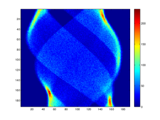
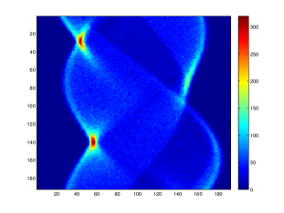
In this section, we present our results on both simulated and real PET data. The Radon matrix that we described in (3.2) is fixed and produces sinograms of size 192×192192192192\times 192, that is the sinogram is given in 192 projection lines, 192osuperscript192𝑜192^{o} degrees with 1osuperscript1𝑜1^{o} degree incrementation and the corresponding reconstructed image is of size 175×175175175175\times 175 pixels. We corrupt the sinograms with Poisson noise of different levels. In order to create noisy images corrupted by Poisson noise, we apply the MATLAB routine imnoise (sinogram, poisson). MATLAB’s imnoise function acts in the following way: for an image of double precision, the input pixel values are interpreted as means of a Poisson distribution scaled by a factor of 1012superscript101210^{-12}. For example, if an input pixel has the value 5.510125.5superscript10125.5*10^{-12} then the corresponding output pixel will be generated from a Poisson distribution with mean of 5.55.55.5 and afterwards scaled back to its original range by 1012superscript101210^{12}. The factor 1012 is fixed to represent the maximal number of detectable photons. Our simulated sinograms are in [0,1]01[0,1] intensity and in order to create different noise levels, we have to rescale the initial sinogram with a suitable factor before applying imnoise and then scale it back with the same factor, i.e., Noisy Sinogram = scale * imnoise ( sinogramscale𝑠𝑖𝑛𝑜𝑔𝑟𝑎𝑚𝑠𝑐𝑎𝑙𝑒\frac{sinogram}{scale}, poisson𝑝𝑜𝑖𝑠𝑠𝑜𝑛poisson ).

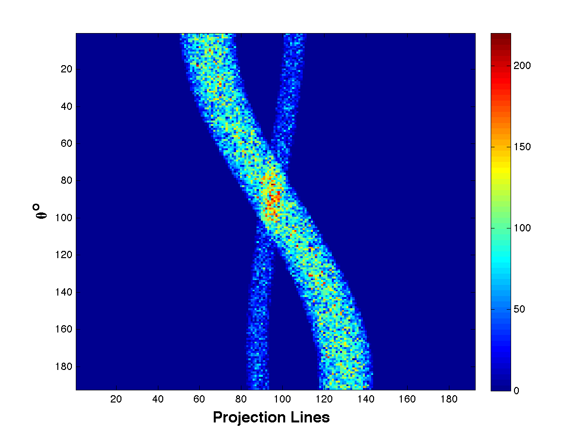
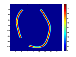
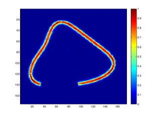
To simulate realistic sinograms with higher noise level, we use 1013superscript101310^{13} as a scaling factor, see for example Figure 5. The real data was obtained from the hardware phantom ”Wilhelm”, a self-built phantom modelled of the human body. Beside the activity in the heart a small source is placed in the phantom to simulate a lesion, see section 4.1 for more information.

Before presenting our results we give some specifics on how equations (3.9)-(3.13) are solved and how parameters are chosen. Both linear systems (3.18) and (3.19) are solved using MATLAB’s built-in function cg which performs a conjugate gradient method. As a stopping criterium we either stop after at most 200200200 iterations or if the relative residual is smaller than 103superscript10310^{-3}. As it is observed in [19], it seems optimal to apply only a few steps of an iterative solver for both subproblems (3.18) and (3.19) since the error in the split Bregman algorithm is updated in every iteration.

The Lagrange multiplies (λi)i=14superscriptsubscriptsubscript𝜆𝑖𝑖14(\lambda_{i})_{i=1}^{4} in equations (3.9)-(3.13) in section 3.2 are chosen following [18] to optimise convergence speed and well conditioning. They were fixed as λ1=0.001subscript𝜆10.001\lambda_{1}=0.001, λ2=1subscript𝜆21\lambda_{2}=1, and λ3=λ4=100subscript𝜆3subscript𝜆4100\lambda_{3}=\lambda_{4}=100. Note that these parameters may affect the condition number for both system matrices

Aimgsubscript𝐴𝑖𝑚𝑔\displaystyle A_{img} =λ1RRλ3div+λ4Iabsentsubscript𝜆1superscript𝑅𝑅subscript𝜆3divsubscript𝜆4𝐼\displaystyle=\lambda_{1}R^{*}R-\lambda_{3}{\rm div}\cdot\nabla+\lambda_{4}I
Asinsubscript𝐴𝑠𝑖𝑛\displaystyle A_{sin} =(1+λ1)gλ2gdivabsent1subscript𝜆1𝑔subscript𝜆2𝑔div\displaystyle=(1+\lambda_{1})g-\lambda_{2}g{\rm div}\cdot\nabla

in (3.18) and (3.19) and hence the convergence rates of iterative solvers used to solve them are affected by this choice.

Finally, we observe that after 150150150 Split Bregman iterations, there are no significant changes in the reconstructed image and therefore we choose a stopping criteria of either at most K=400𝐾400K=400 iterations or we stop at iteration K𝐾K where for the first time we have

u~K+1u~K2u~K+12<104subscriptdelimited-∥∥superscript~𝑢𝐾1superscript~𝑢𝐾2subscriptdelimited-∥∥superscript~𝑢𝐾12superscript104\frac{\left\lVert\widetilde{u}^{K+1}-\widetilde{u}^{K}\right\rVert_{2}}{\left\lVert\widetilde{u}^{K+1}\right\rVert_{2}}<10^{-4}

where u~K+1superscript~𝑢𝐾1\widetilde{u}^{K+1} the regularised image. To evaluate the quality of reconstructed images we choose the Signal-to-Noise Ratio (SNR) as a quality measure. The SNR is defined as

SNR=20log(u2uu~2)𝑆𝑁𝑅20subscriptdelimited-∥∥𝑢2subscriptdelimited-∥∥𝑢~𝑢2SNR=20\log\bigg{(}\frac{\left\lVert u\right\rVert_{2}}{\left\lVert u-\widetilde{u}\right\rVert_{2}}\bigg{)} (4.1)

where u𝑢u and u~~𝑢\widetilde{u} denote the ground truth and the reconstructed image, respectively. In what follows, we first evaluate the proposed reconstruction technique (2.1) against pure total variation regularisation on the image (β=0𝛽0\beta=0) for a synthetic image of two circles and for different noise levels, as well as for a real data set acquired for the Wilhelm phantom. Then, we numerically analyse the scale space properties of pure sinogram regularisation, that is for α=0𝛼0\alpha=0, which will be a motivation for the final section in which we discuss the merit of the proposed reconstruction method for PET data that encodes thin image structures.

4.1 Image reconstruction from corrupted simulated and real PET data

We start with a discussion of numerical results obtained for simulated PET data. Figure 5 shows a simulated phantom of two discs with different radius and the corresponding noiseless and noisy sinograms corrupted with low and high level Poisson noise as described above.
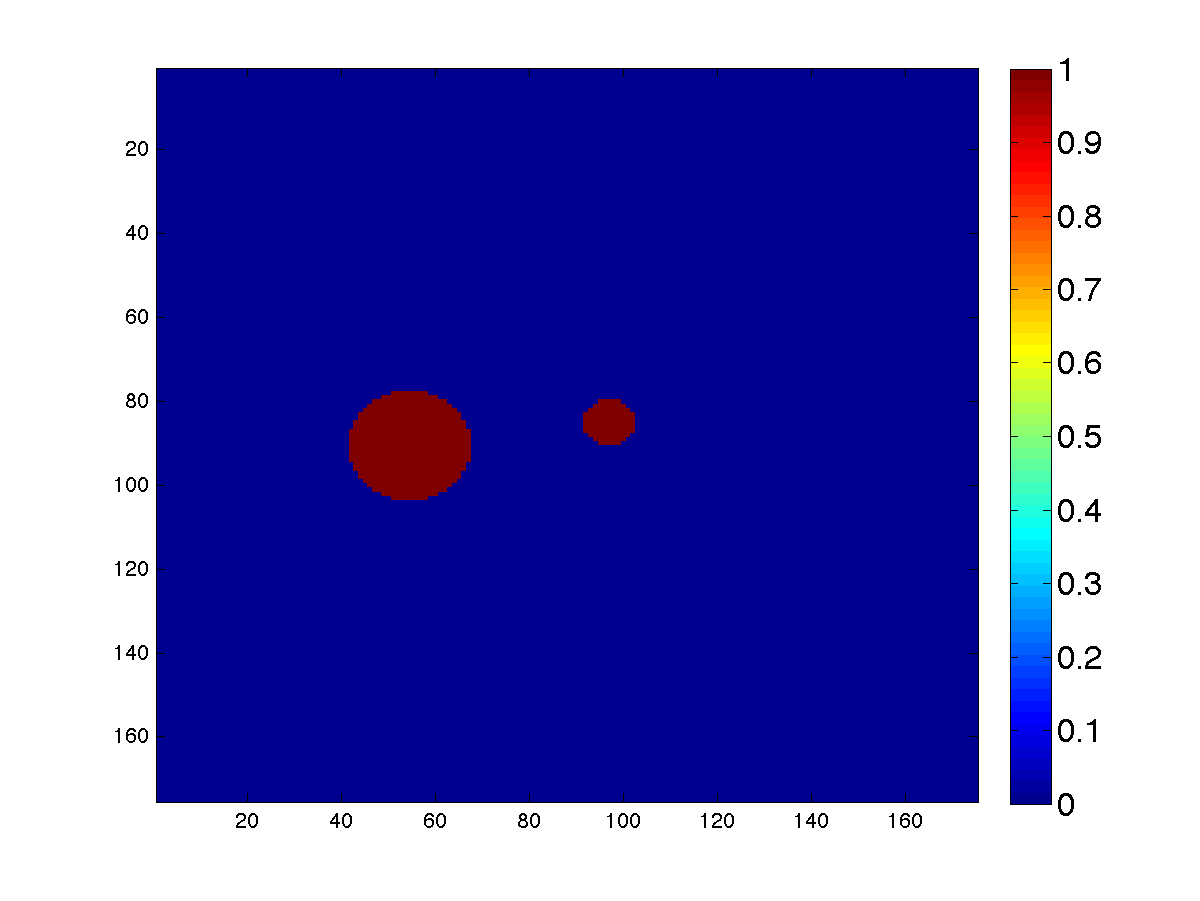
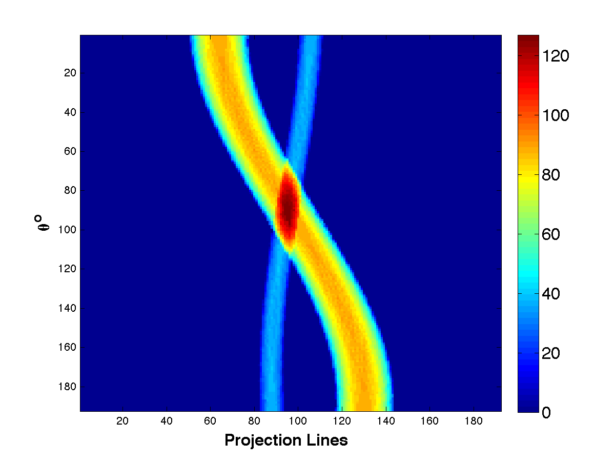
Refer to caption
(a) 2 discs
 
Refer to caption
(b) Noiseless Sinogram
Refer to caption
(c) Low Noise: SNR=18.5246
Refer to caption
(d) High Noise: SNR=8.6814
Fig. 5: The phantom image includes 2 discs of radius r1=26subscript𝑟126r_{1}=26 and r2=11subscript𝑟211r_{2}=11 pixels. Its sinogram has 192 angles and 192192192 rays with low and high noise.

First, we evaluate the proposed algorithm for reconstructing an image from the sinogram corrupted by low level Poisson noise with SNR=18.5246, see Figure (5(c)). The proposed reconstruction algorithm with joint total variation regularisation of image and sinogram (that is α,β>0𝛼𝛽0\alpha,\beta>0) is compared with the algorithm that uses pure total variation regularisation of the image (that is α>0𝛼0\alpha>0 and β=0𝛽0\beta=0). Both reconstruction strategies are tested for a range of parameters α,β𝛼𝛽\alpha,\beta and in each case the reconstruction is found which has the highest SNR value. For β=0𝛽0\beta=0 we computed the reconstructed image for α=3,4,5,6,7𝛼34567\alpha=3,4,5,6,7. The optimal reconstructed image in terms of the best SNR=25.8589absent25.8589=25.8589 is obtained for α=6𝛼6\alpha=6, see Figure 6. Then, we test the proposed reconstruction method applying total variation regularisation on both the image and the sinogram using the same range of α=3,4,5,6,7𝛼34567\alpha=3,4,5,6,7 and β=0.001,0.005,0.01,0.05𝛽0.0010.0050.010.05\beta=0.001,0.005,0.01,0.05. Here, the optimal reconstruction was obtained for α=6𝛼6\alpha=6 and β=0.001𝛽0.001\beta=0.001 with SNR=25.3127absent25.3127=25.3127, see Figure 6. In Table 1 a full list of tested parameters and SNRs for corresponding reconstructed images is given. The results do not indicate a significant difference between the algorithm with and without total variation regularisation on the sinogram, both visually and also in terms of the SNR. Indeed, in the low noise case additional total variation regularisation on the sinogram produces even slightly worse results in terms of SNR than using no regularisation on the sinogram at all.
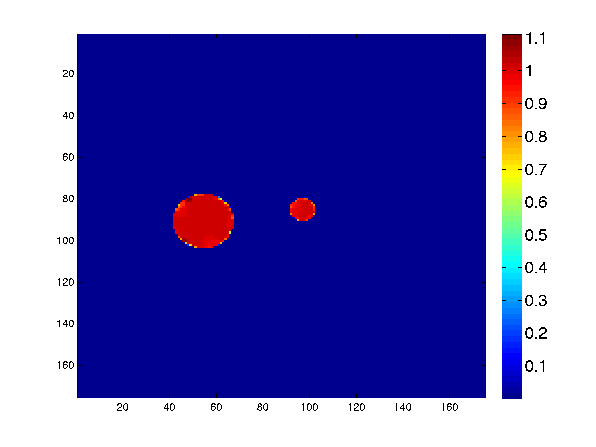
Refer to caption
(a) α=6𝛼6\alpha=6, β=0𝛽0\beta=0
SNR=25.8589
Refer to caption
(b) α=6𝛼6\alpha=6, β=103𝛽superscript103\beta=10^{-3}
SNR=25.3127
Refer to caption
(c) Middle line profiles
Fig. 6: Low Level Noise: Optimal reconstruction results of the 2 discs image with sinogram shown in Figure (5(c)) with and without sinogram regularisation and a comparison of the line profiles for the two results.
β𝛽\beta
0 0.001 0.005 0.01 0.05 0.1
α𝛼\alpha 3 24.0819 22.0172 22.4415 22.8894 23.2414 21.6533
4 25.3682 24.0926 24.2951 24.4801 23.6303 21.9382
5 25.7867 25.0829 25.0779 25.0469 23.9432 22.0367
6 25.8589 25.3127 24.7787 25.0602 24.0095 22.1034
7 25.7436 24.8499 24.8278 25.0148 23.9662 22.2289
Table 1: Low Level Noise for simulated example in Figure 5: SNRs of reconstructed images for different combinations of α𝛼\alpha and β𝛽\beta values.

The TV regularisation on the sinogram gains importance in the reconstruction algorithm when the noise in the corruption of the sinogram is increased. The sinogram with high level noise is shown in Figure (5(d)) and has SNR=8.6814. We tested the proposed method for α=250,275,300,325,350𝛼250275300325350\alpha=250,275,300,325,350 and β=0,0.001,0.01,0.05,0.1𝛽00.0010.010.050.1\beta=0,0.001,0.01,0.05,0.1. The results are reported in Table 2.

β𝛽\beta
0 0.001 0.005 0.01 0.05 0.1
α𝛼\alpha 250 10.9544 10.9665 10.9557 10.9464 10.8531 10.8058
275 10.9502 10.9599 10.9501 10.9381 10.8595 10.8013
300 10.9425 10.9543 10.9415 10.9257 10.8267 10.7777
325 10.9167 10.9551 10.9434 10.9283 10.8101 10.7293
350 10.8784 10.9289 10.9165 10.9014 10.7946 10.7104
Table 2: High Level Noise for simulated example in Figure 5: SNRs of reconstructed images for different combinations of α𝛼\alpha and β𝛽\beta values.
Refer to caption
(a) α=250𝛼250\alpha=250, β=0𝛽0\beta=0
SNR=10.9544
Refer to caption
(b) α=250𝛼250\alpha=250, β=103𝛽superscript103\beta=10^{-3}
SNR=10.9665
Refer to caption
(c) Zoom In: Middle line profiles
Fig. 7: High Level Noise for simulated example in Figure 5: Best SNRs with/without total variation regularisation on the sinogram and the middle line profiles of the reconstructed images.

The highest SNR is obtained when α=250𝛼250\alpha=250 and β=0.001𝛽0.001\beta=0.001, cf. Figure (7(b)). Although, it is hard to distinguish any difference between the cases of β𝛽\beta, we observe that the extra penalisation on the sinogram produces better results in terms of the SNR value, see Figure 7. The increase in SNR for β>0𝛽0\beta>0 can be seen when comparing the middle line profiles of the reconstructed images with and without sinogram regularisation in Figure (7(c)).

As a second example for our evaluation of the algorithm for PET reconstruction we consider real PET data obtained from scanning a self-built phantom of a human breast with a small source which simulates a lesion, compare Figure (8(a)). The data has been acquired with a Siemens Biograph Sensation 16 PET/CT scanner (Siemens Medical Solutions) located at the University Hospital in Münster. From the 3D PET data we used only one sinogram slice. The 2D sinogram dimension is 192×192192192192\times 192 with a pixel size of 3.375mm23.375𝑚superscript𝑚23.375mm^{2}. The size of the reconstructed image is 175×175175175175\times 175, covering a field of view of 590.625mm590.625𝑚𝑚590.625mm in diameter. The 2D slice of the noisy sinogram which has been used in our computations is shown in Figure (8(b)). Reconstructions obtained from the proposed algorithm, with and without sinogram regularisation, are shown in Figure 9. The additional regularisation of the sinogram seems to allow for smoother image structures (such as the boundary of the red lesion) and results in a slight reduction of the stair casing effect of total variation regularisation.
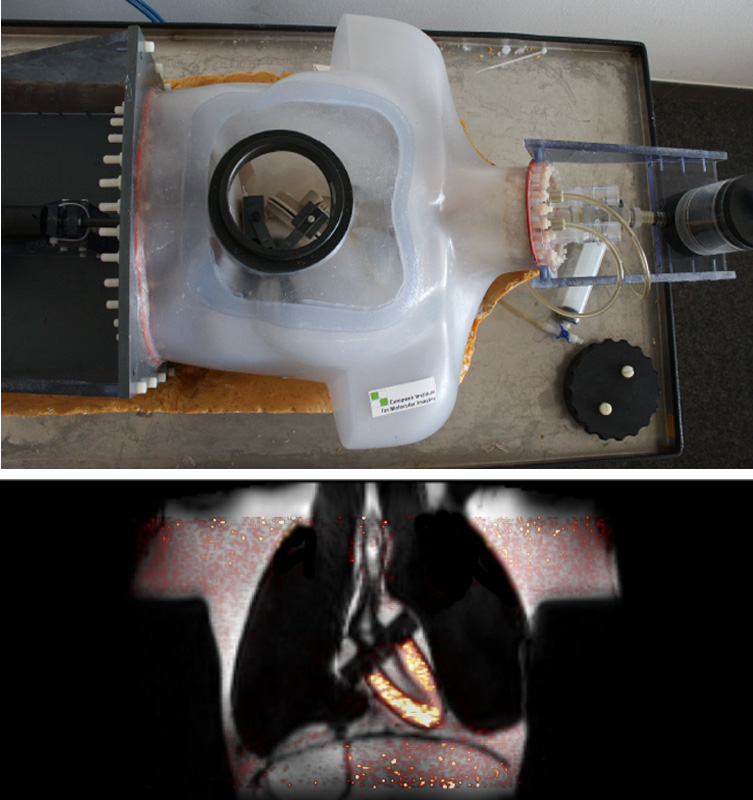
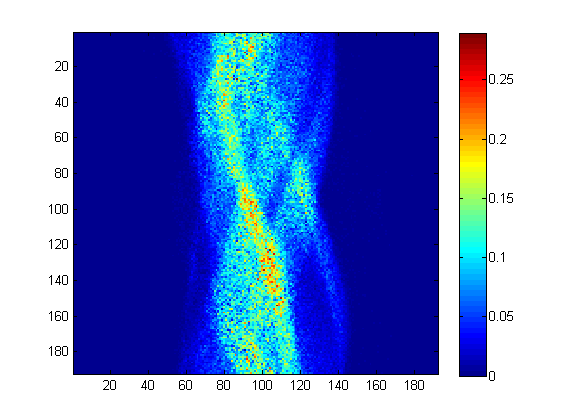
Refer to caption
(a) Top: Phantom ”Wilhelm”, consisting of a plastic torso and inserts for the lungs, heart and liver. Bottom: Phantom reconstruction with combined PET-MRI. Data courtesy of the European Institute for Molecular Imaging (EIMI), Münster.
Refer to caption
(b) Noisy sinogram.
Fig. 8: Real PET data.
Refer to caption
(a) α=5𝛼5\alpha=5, β=0𝛽0\beta=0
Refer to caption
(b) α=4𝛼4\alpha=4, β=0.1𝛽0.1\beta=0.1
Fig. 9: Real Data: Best TV regularised reconstructions for noisy slice in Figure 8(b).

In the following two sections we will aim to improve our understanding of this new sinogram regularisation, taking the analytic solution of section 2.5 as a starting point. A thorough numerical discussion of this example in section 4.2 leeds us to section 4.3 where the benefits of total variation regularisation of the sinogram for the reconstruction of thin objects are discussed.

4.2 Scale space of sinogram regularisation

Following up on the computations in section 2.5, we now discuss how the regularisation on the sinogram effects the backprojected image. Let us recall that every point (θ,s)𝜃𝑠(\theta,s) on the sinogram corresponds to a line s=xcosθ+ysinθ𝑠𝑥𝜃𝑦𝜃s=x\cos\theta+y\sin\theta that passes through a point (x,y)𝑥𝑦(x,y) on the image, with a distance s𝑠s from the origin and normal to the direction (cosθ,sinθ)𝑐𝑜𝑠𝜃𝜃(cos\theta,\sin\theta). Moreover (compare Thirion [34]), every point on an edge in the sinogram corresponds to a line in the object space which is tangent to the boundary of the object. To further understand how sinogram regularisation acts, we consider the effect of the regularisation when reconstructing an image from simulated noise-free Radon data. To this end we set α=0𝛼0\alpha=0, regularise the noise-free sinogram with different values of β𝛽\beta, and apply FBP to the regularised sinogram to obtain the corresponding reconstructed image. We call the set of reconstructed images from regularised sinograms with varying β𝛽\beta regularisation, the scale space of total variation regularisation of the sinogram.

Considering the reconstruction method (2.1) for α=0𝛼0\alpha=0 results in the following weighted total variation denoising problem for the sinogram g𝑔g

argminv0 a.e βv1+k,l(gv)2gsubscriptargmin𝑣0 a.e 𝛽subscriptdelimited-∥∥𝑣1subscript𝑘𝑙superscript𝑔𝑣2𝑔\operatorname*{arg\,min}_{v\geq 0\mbox{ a.e }}\beta\left\lVert\nabla v\right\rVert_{1}+\sum_{k,l}\frac{(g-v)^{2}}{g} (4.2)

where 1subscriptdelimited-∥∥1\left\lVert\cdot\right\rVert_{1} is the discrete l1superscript𝑙1l^{1} norm as defined before. Similar to before, we solve (4.2) by a Split Bregman technique, introducing two more variables w=v𝑤𝑣w=\nabla v and v~=v~𝑣𝑣\widetilde{v}=v. Then, starting with initial conditions b102k×lsuperscriptsubscript𝑏10superscript2𝑘𝑙b_{1}^{0}\in\mathbb{R}^{2k\times l} and b20k×lsuperscriptsubscript𝑏20superscript𝑘𝑙b_{2}^{0}\in\mathbb{R}^{k\times l}, we iteratively solve for k=1,2,𝑘12k=1,2,\ldots

vk+1superscript𝑣𝑘1\displaystyle v^{k+1} =argminvλ12b1k+vwk22+λ22b2k+vv~k22absentsubscriptargmin𝑣subscript𝜆12superscriptsubscriptdelimited-∥∥superscriptsubscript𝑏1𝑘𝑣superscript𝑤𝑘22subscript𝜆22superscriptsubscriptdelimited-∥∥superscriptsubscript𝑏2𝑘𝑣superscript~𝑣𝑘22\displaystyle=\operatorname*{arg\,min}_{v}\frac{\lambda_{1}}{2}\left\lVert b_{1}^{k}+\nabla v-w^{k}\right\rVert_{2}^{2}+\frac{\lambda_{2}}{2}\left\lVert b_{2}^{k}+v-\widetilde{v}^{k}\right\rVert_{2}^{2} (4.3)
v~k+1superscript~𝑣𝑘1\displaystyle\widetilde{v}^{k+1} =argminv~012(gv~)2g+λ22b2k+vk+1v~22absentsubscriptargmin~𝑣012superscript𝑔~𝑣2𝑔subscript𝜆22superscriptsubscriptdelimited-∥∥superscriptsubscript𝑏2𝑘superscript𝑣𝑘1~𝑣22\displaystyle=\operatorname*{arg\,min}_{\widetilde{v}\geq 0}\frac{1}{2}\int\frac{(g-\widetilde{v})^{2}}{g}+\frac{\lambda_{2}}{2}\left\lVert b_{2}^{k}+v^{k+1}-\widetilde{v}\right\rVert_{2}^{2} (4.4)
wk+1superscript𝑤𝑘1\displaystyle w^{k+1} =argminwβw1+λ12b1k+vk+1w22absentsubscriptargmin𝑤𝛽subscriptdelimited-∥∥𝑤1subscript𝜆12superscriptsubscriptdelimited-∥∥superscriptsubscript𝑏1𝑘superscript𝑣𝑘1𝑤22\displaystyle=\operatorname*{arg\,min}_{w}\beta\left\lVert w\right\rVert_{1}+\frac{\lambda_{1}}{2}\left\lVert b_{1}^{k}+\nabla v^{k+1}-w\right\rVert_{2}^{2} (4.5)
b1k+1superscriptsubscript𝑏1𝑘1\displaystyle b_{1}^{k+1} =b1k+wk+1vk+1absentsuperscriptsubscript𝑏1𝑘superscript𝑤𝑘1superscript𝑣𝑘1\displaystyle=b_{1}^{k}+\nabla w^{k+1}-v^{k+1} (4.6)
b2k+1superscriptsubscript𝑏2𝑘1\displaystyle b_{2}^{k+1} =b2k+vk+1v~k+1absentsuperscriptsubscript𝑏2𝑘superscript𝑣𝑘1superscript~𝑣𝑘1\displaystyle=b_{2}^{k}+v^{k+1}-\widetilde{v}^{k+1} (4.7)

Note that, as before, in the solution of (3.19) a simple backprojection of the sinogram is used and we set λ1=λ2=1subscript𝜆1subscript𝜆21\lambda_{1}=\lambda_{2}=1. Moreover, since we do not apply any positivity constraint on the image as it is done in the full algorithm used in section 4.1, we might observe small negative values in the reconstructed images presented in the following.
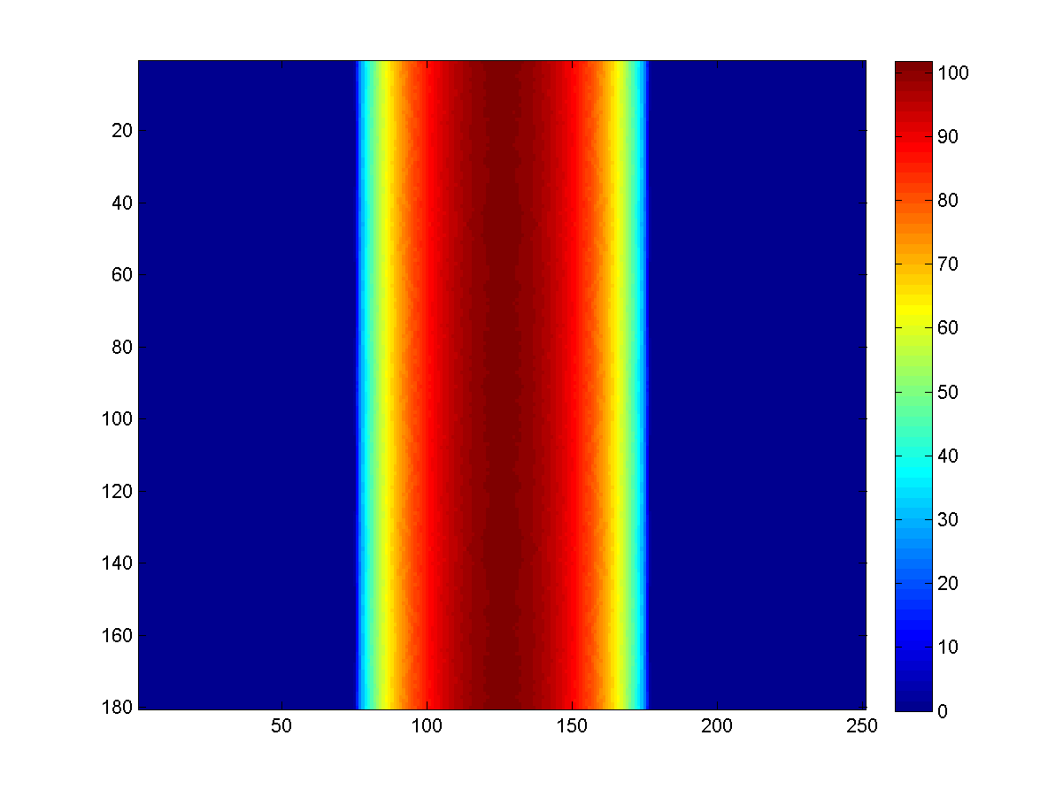
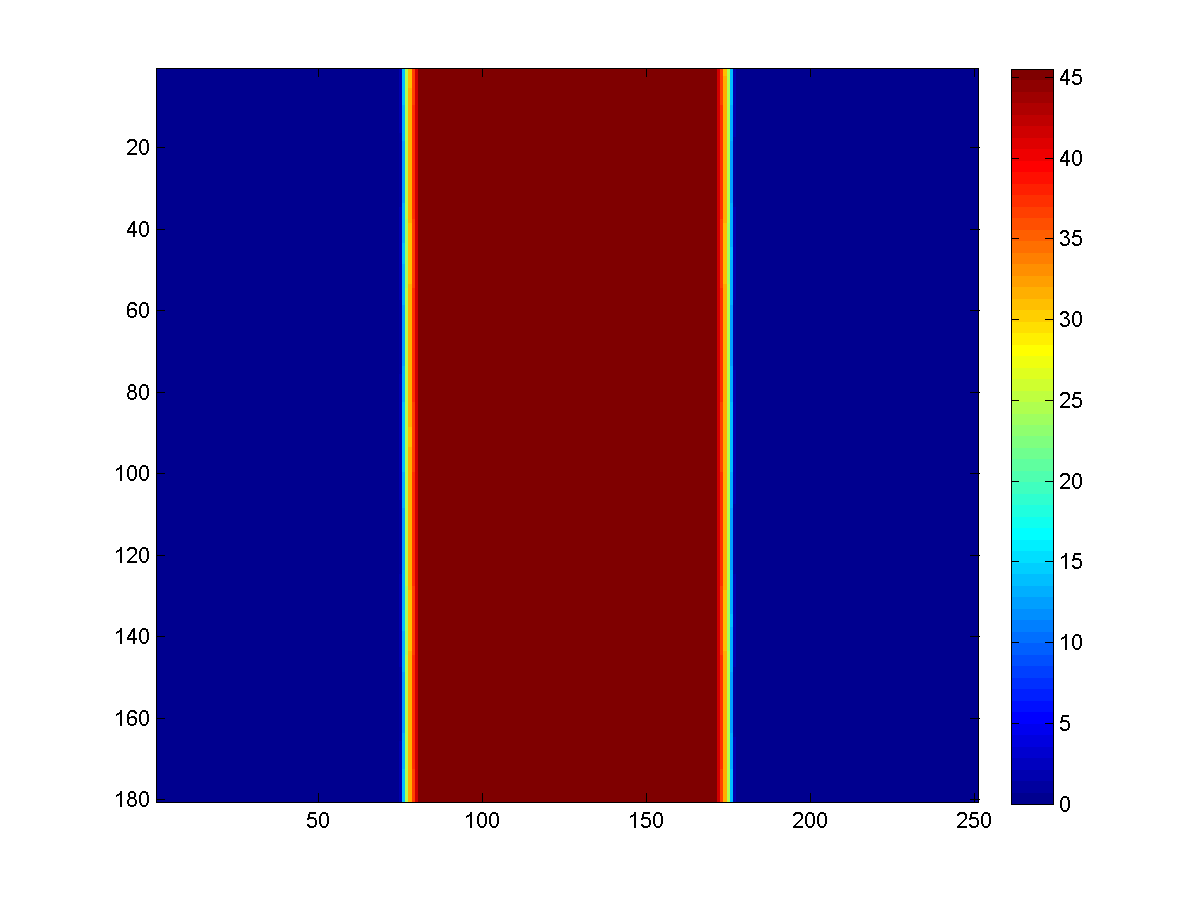
(a) β=103𝛽superscript103\beta=10^{-3}
Refer to caption
(b) β𝛽\beta=20
Refer to caption
(c) β𝛽\beta=45
Refer to caption
(d) β𝛽\beta=50.5
Refer to caption
Refer to caption
Refer to caption
Refer to caption
Refer to caption
Refer to caption
Refer to caption
Refer to caption
Refer to caption
Refer to caption
Refer to caption
Refer to caption
Refer to caption
Fig. 10: Sinogram regularisation with different values of β𝛽\beta (first row) and the corresponding filtered backprojected images (third row). The second row represents a 45osuperscript45𝑜45^{o} comparison of the original sinogram and the sinogram after regularisation. The highest value of the sinogram is 102.8102.8102.8. The fourth row represents the middle line profiles of the reconstructed images in the third row.

First, we consider image functions with radial symmetry such as in section 2.5 equation (2.30). Figure 10 shows the numerically computed regularised sinograms and corresponding images for an original image of a disc with radius r=50.5𝑟50.5r=50.5. Here we have used MATLAB’s built-in function iradon with a Ram-Lak filter and spline interpolation to compute the FBP of the regularised sinogram. Moreover, Table 3, shows the correspondence of the numerical solution with the analytic solution in section 2.5 for three discs of radii r=15.5,30.5𝑟15.530.5r=15.5,30.5 and 50.550.550.5. Here, δansuperscript𝛿𝑎𝑛\delta^{an} and δnumsuperscript𝛿𝑛𝑢𝑚\delta^{num} denote the analytic and numerical δ𝛿\delta, respectively, in the expression of the regularised solution in (2.30). As predicted from the computations in section 2.5, we see that with increasing regularisation parameter β𝛽\beta the regularised image more and more emphasises the boundary of the disc.

r=15.5𝑟15.5r=15.5 β𝛽\beta 103superscript10310^{-3} 0.1 1 5 10 15 15.5
δansuperscript𝛿𝑎𝑛\delta^{an} 30.94 29.88 25.84 16.09 7.59 0.64 0.084
δnumsuperscript𝛿𝑛𝑢𝑚\delta^{num} 31.32 29.76 25.71 15.96 7.37 0.67 0.37
r=30.5𝑟30.5r=30.5 β𝛽\beta 103superscript10310^{-3} 1 10 15 20 25 30.5
δansuperscript𝛿𝑎𝑛\delta^{an} 60.93 59.6 31.35 22.37 14.46 7.27 0.09
δnumsuperscript𝛿𝑛𝑢𝑚\delta^{num} 61.98 54.58 31.42 22.47 14.55 7.34 0.65
r=50.5𝑟50.5r=50.5 β𝛽\beta 103superscript10310^{-3} 1 10 20 30 45 50.5
δansuperscript𝛿𝑎𝑛\delta^{an} 100.92 93.33 65.74 45.46 28.71 7.16 0.12
δnumsuperscript𝛿𝑛𝑢𝑚\delta^{num} 101.83 93.26 65.75 45.41 28.82 7.24 0.68
Table 3: Comparison of analytic and numerical computations of sinogram regularisation for three test images of characteristic functions of circles with radii r=15.5,30.5𝑟15.530.5r=15.5,30.5 and 50.550.550.5. The parameters δansuperscript𝛿𝑎𝑛\delta^{an} and δnumsuperscript𝛿𝑛𝑢𝑚\delta^{num} denote the analytic and numerical δ𝛿\delta, respectively, in the expression of the regularised solution in (2.30). Compare also Figure 10 for regularised reconstructions for the circle with radius r=50.5𝑟50.5r=50.5.

Going beyond radial symmetry we consider three additional examples where the sinogram depends on the angle θ𝜃\theta. First, we simply consider the image that we used in the previous section in Figure 5 without adding additional noise to its sinogram. The effect of β𝛽\beta regularisation in this case is presented in Figure 11. We see that as we increase β𝛽\beta we loose details in the image, starting again from the inner structure of the discs, while enhancing the boundaries of the objects. Here, the connection of the choice of β𝛽\beta with the radius of every circle is clearly visible. More precisely, for β<r2𝛽subscript𝑟2\beta<r_{2} the boundary of the smaller circle is enhanced and for r2<β<r1subscript𝑟2𝛽subscript𝑟1r_{2}<\beta<r_{1} the small circle is lost and the boundary of the larger circle is enhanced.
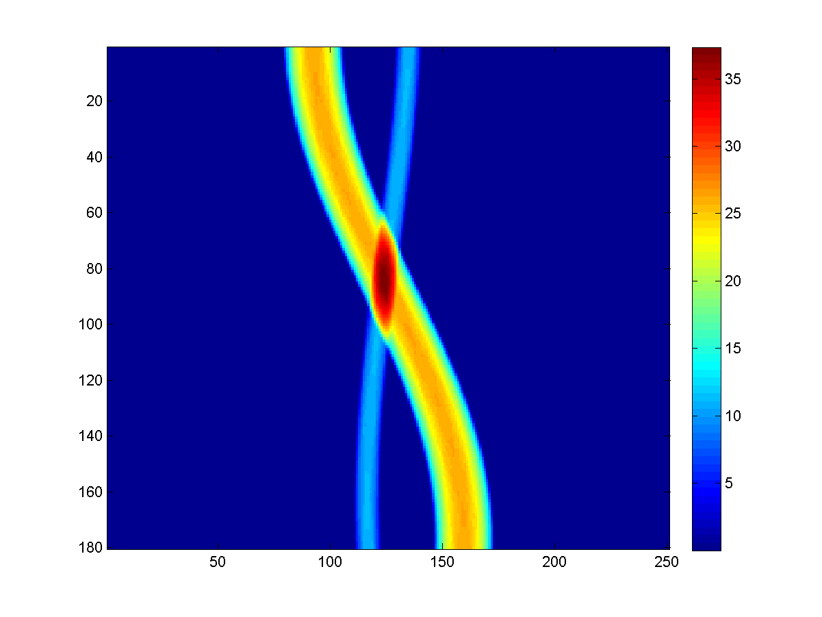
(a) β=103𝛽superscript103\beta=10^{-3}
Refer to caption
(b) β𝛽\beta=1
Refer to caption
(c) β𝛽\beta=3
Refer to caption
(d) β𝛽\beta=7
Refer to caption
(e) β𝛽\beta=12
Refer to caption
Refer to caption
Refer to caption
Refer to caption
Refer to caption
Refer to caption
Fig. 11: Sinogram regularisation with different values of β𝛽\beta and the corresponding filtered backprojected images using MATLAB’s iradon built-in function. The radii for the discs are r1=13subscript𝑟113r_{1}=13 and r2=5.5subscript𝑟25.5r_{2}=5.5.
Refer to caption
(a) 2 rings
Refer to caption
(b) Sinogram
Refer to caption
(c) Star
Refer to caption
(d) Sinogram
Fig. 12: 2 rings with different annulus regions and its sinogram ((a) and (b)), star-shaped image of 5 points and its sinogram ((c) and (d)).

In Figure 12, we present two more test images. The first one is an image of two rings with the same outer radius but with different annulus regions, compare Figure (12(a)). A similar scale-space analysis as for the previous examples is carried out in Figure 13. Additionally to the enhancement of the outer boundaries of the two rings we see that for increasing β𝛽\beta regularisation the reconstructed image approaches the convex hull of the two rings. This is even more apparent for the last example of a star-shaped object in Figure (12(c)). See Figure 14 in particular.
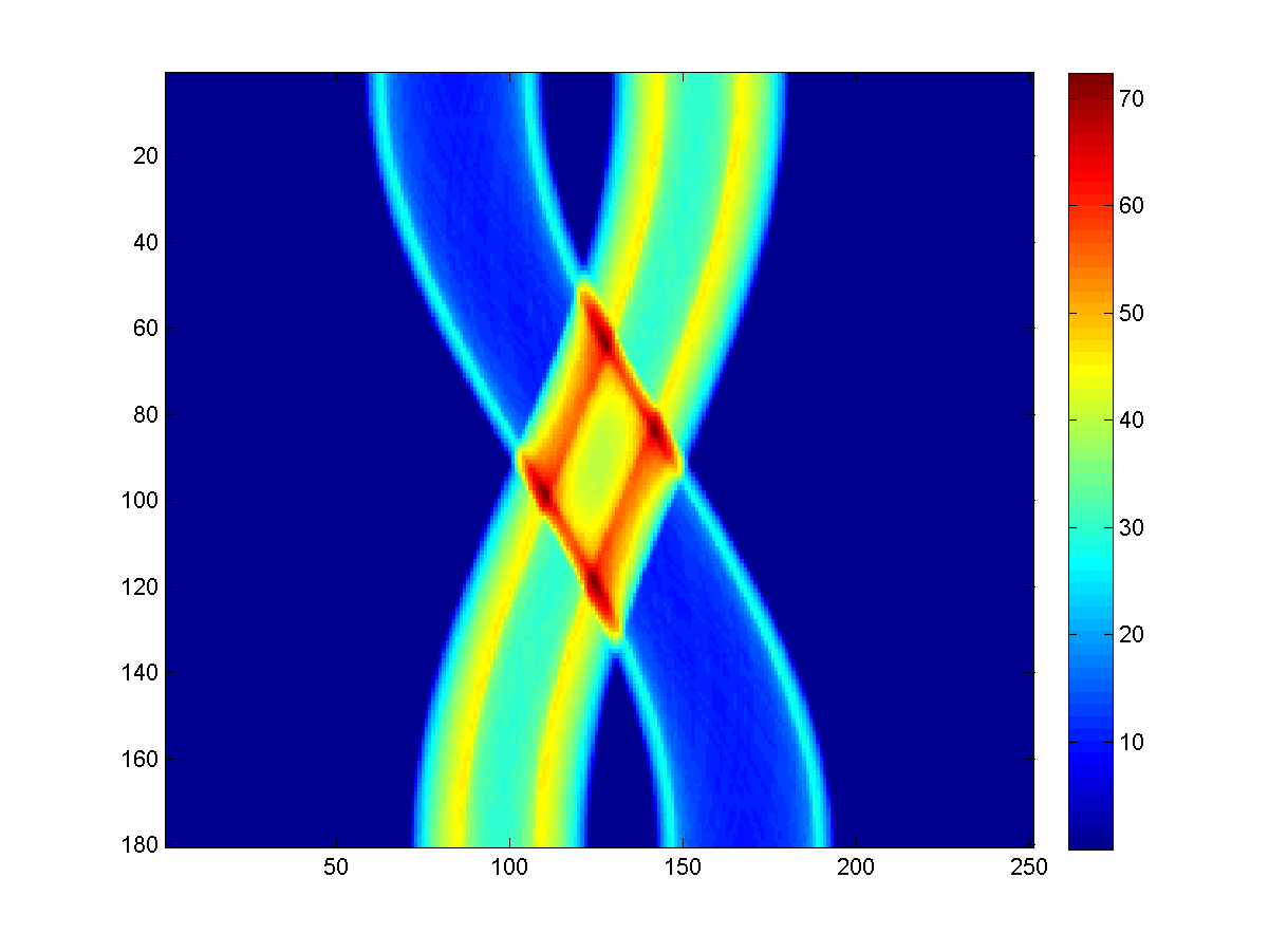
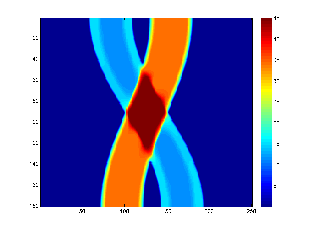
(a) β𝛽\beta=0.001
Refer to caption
(b) β𝛽\beta=1
Refer to caption
(c) β𝛽\beta=10
Refer to caption
(d) β𝛽\beta=25.5
Refer to caption
Refer to caption
Refer to caption
Refer to caption
Refer to caption
Fig. 13: 2 rings with different annulus regions: The outer radius for both rings is r=25.5 and the inner radii are r1=21subscript𝑟121r_{1}=21 and r2=11subscript𝑟211r_{2}=11. For figures (a)-(d), we present the sinogram regularisation for increasing values of β𝛽\beta with the corresponding filtered backprojected using MATLAB’s iradon built-in function.
(a) β𝛽\beta=0.001
Refer to caption
(b) β𝛽\beta=0.1
Refer to caption
(c) β𝛽\beta=1
Refer to caption
(d) β𝛽\beta=10
Refer to caption
(e) β𝛽\beta=50
Refer to caption
Refer to caption
Refer to caption
Refer to caption
Refer to caption
Refer to caption
Fig. 14: Star-shaped image of 5 corners: In Figures (a)-(d), we present the sinogram regularisation for increasing values of β𝛽\beta with the corresponding filtered backprojected image using MATLAB’s built-in function iradon.

The conclusion of this section is the motivation for the next section at the same time. Analysing the effect of total variation regularisation on the sinogram by considering its scale space and its effect on the reconstructed image we have seen in Figure 1014 the potential use of this method for the enhancement and detection of object boundaries. As we will see in the next section, this effect can be exploited for enhancing thin structures in images obtained from Radon measurements.

4.3 Thin Structure Reconstruction

In what follows, we discuss how total variation regularisation of the sinogram can improve the quality of the reconstruction in comparison with pure total variation regularisation of the image in the presence of thin structures in the image. Our first example is a thin rectangular frame in Figure 15. Similarly as in section 4.1, we start by finding an optimal value of α𝛼\alpha with β=0𝛽0\beta=0, in terms of SNR. Then, we select a range of α𝛼\alpha values close to this optimal one and we allow strictly positive values for β𝛽\beta. The noise that is added on the sinogram, is generated by MATLAB’s imnoise routine, with a 1012superscript101210^{12} scaling factor, see the beginning of section 4 for more explanation. The test image that is shown in Figure 15 has 50 pixels width and 100 pixels length and the rectangular frame has a width of 2 pixels. In Figure 16, we first present some of the results obtained with pure total variation regularisation on the image, that is when β=0𝛽0\beta=0. As we increase the α𝛼\alpha parameter, we observe that the best SNR corresponds to α𝛼\alpha=5 with SNR=19.9764. That is because for small values of α𝛼\alpha we observe that the large-scale structure of the object is still intact, with the cost that noise is still present in the reconstructed image, see Figures 16 (16(a))-(16(c)). However, with higher values of α𝛼\alpha noise is further eliminated but at the expense of a significant loss of contrast and some unpleasant artifacts along the boundaries of the frame, see Figure 16 (16(d))-(16(f)).
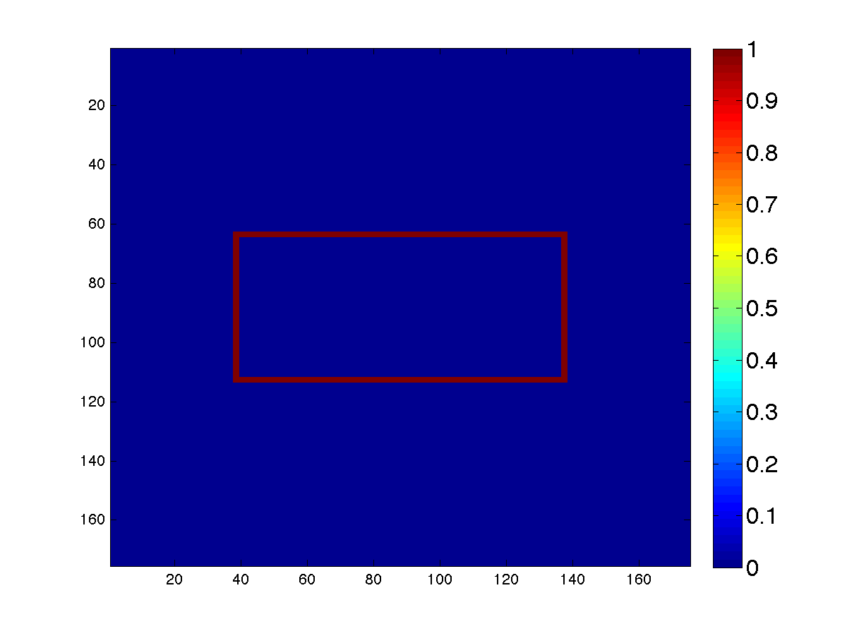
Refer to caption
(a) Thin Rectangle
Refer to caption
(b) Noiseless Sinogram
Refer to caption
(c) Low noise: SNR=14.9146
Fig. 15: A thin rectangle of 50 pixels width and 100 pixels length with 2 pixels length on the boundaries. The corresponding noiseless and noisy sinograms with 1012superscript101210^{12} scaling factor in imnoise.
Refer to caption
(a) α=1𝛼1\alpha=1, β=0𝛽0\beta=0
SNR=16.5399
Refer to caption
(b) α=5𝛼5\alpha=5, β=0𝛽0\beta=0
SNR=19.9764
Refer to caption
(c) α=10𝛼10\alpha=10, β=0𝛽0\beta=0
SNR=19.8700
Refer to caption
(d) α=20𝛼20\alpha=20, β=0𝛽0\beta=0
SNR=16.2678
Refer to caption
(e) α=30𝛼30\alpha=30, β=0𝛽0\beta=0
SNR=13.054
Refer to caption
(f) α=50𝛼50\alpha=50, β=0𝛽0\beta=0
SNR=8.6456
Fig. 16: Thin Rectangle: Reconstruction without total variation regularisation on the sinogram and different parameters of α𝛼\alpha.
β𝛽\beta
0 0.005 0.01 0.05 0.1
α𝛼\alpha 2 17.6798 18.0078 19.7238 24.5981 24.2978
3 18.6444 18.9855 20.6460 23.9028 24.2647
4 19.4269 19.7539 21.5305 23.9178 23.2860
5 19.9764 20.2979 21.7962 23.6466 22.8525
6 20.2583 20.5771 21.9057 23.2213 22.3440
7 20.4471 20.8665 21.8372 22.7554 21.8147
8 20.3511 20.3276 20.9859 22.2391 21.2477
Table 4: Thin Rectangle: SNR with β0𝛽0\beta\neq 0.
Refer to caption
(a) α=7𝛼7\alpha=7, β=0𝛽0\beta=0
SNR=20.4471
Refer to caption
(b) α=2𝛼2\alpha=2, β=0.05𝛽0.05\beta=0.05
SNR=24.5981
Fig. 17: Thin Rectangle: Best reconstructions with and without total variation regularisation on the sinogram as reported in Table 4.

If we switch on total variation regularisation on the sinogram, that is taking β>0𝛽0\beta>0, we obtain results which are greatly improved both in terms of the SNR of the reconstructed images but also – visually – in terms of finding the right balance of eliminating the noise and accurately preserving the thin structures, see Table 4 and Figure 17. This observation is confirmed by a second example of an image of two thin straight lines which cross, compare Figure 18. The width of the thin lines is 3 pixels. The length of the horizontal line is 121 pixels and of the vertical line is 100 pixels. The noise, added on the sinogram, is generated with the same scaling factor of 1012superscript101210^{12} as before. Again, we observe that for positive values of β𝛽\beta, we obtain much better reconstructions with almost all noise eliminated while keeping the boundaries of the thin structures intact, see Figure 19.

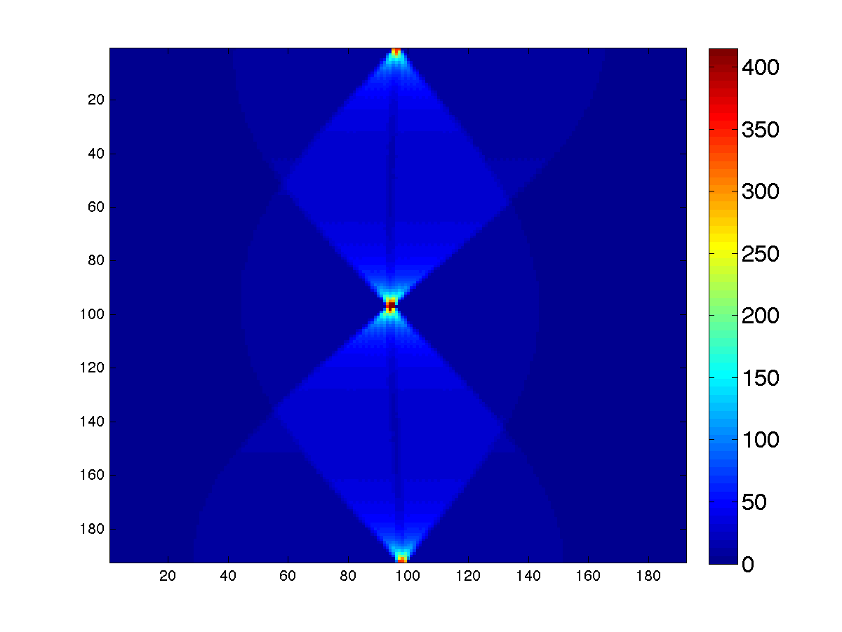
Refer to caption
(a) Cross
Refer to caption
(b) Sinogram
Refer to caption
(c) SNR=16.1538
Fig. 18: Test image of two thin crossing lines and its noiseless and noisy sinograms respectively.
Refer to caption
(a) α=7𝛼7\alpha=7, β=0𝛽0\beta=0
SNR=20.6859
Refer to caption
(b) α=5𝛼5\alpha=5, β=0.05𝛽0.05\beta=0.05
SNR=22.8333
Fig. 19: Reconstruction for the noisy sinogram in Figure 18 that correspond to the best SNR for both cases of β𝛽\beta.
Refer to caption
Fig. 20: XCAT phantom

We also apply our method to a more realistic PET phantom for visualising activity of the human heart. The XCAT phantom is a 3D phantom. For our purpose we used one z-slice through the centre of the phantom which represents a transverse plane view of the human body, see Figure (20). In particular, we can see the activity of the heart through the myocardium (the muscle surrounding the heart) in red. We focus on regions where thin structures are observed, see Figure (21(a))-(21(b)) and add the usual level of Poisson noise to their corresponding sinograms, see Figure (21(c))-(21(d)). In Figures (22(a))-(22(d)) we present our best reconstructions for these two different data-regions in terms of the SNR values for both cases of with and without sinogram regularisation. It is obvious that the best reconstructions are achieved when there is no regularisation on the sinogram. That is because for increasing values of β𝛽\beta a smoothing on the originally blocky boundaries is enforced and hence the SNR value is reduced. Indeed, as we show in the following experiments this is only true if the initial data that we start our experiments with is of low resolution and the thin structures have blocky instead of smooth boundaries. If we change our experiment to the consideration of a high resolution version of the XCAT phantom with thin structures as in Figures (21(a))-(21(b)) but with medically more realistic smooth boundaries, the positive effect of the TV sinogram regularisation can be observed. As it is expected, regularising only on the image space creates a rather unpleasant staircasing effect along the boundaries which is clearly eliminated when we combine the regularisation on both spaces, see Figure 24. Indeed, a significant increase of the SNR when turning on the TV regularisation on the sinogram (β>0𝛽0\beta>0) can be observed.

Refer to caption
(a) Zoom in
Refer to caption
(b) Zoom in
Refer to caption
(c) Noisy sinogram of (a)
Refer to caption
(d) Noisy sinogram of (b)
Fig. 21: Selected regions of the XCAT phantom with the corresponding noisy sinograms.
Refer to caption
(a) α=5𝛼5\alpha=5, β=0𝛽0\beta=0
SNR=17.49887
Refer to caption
(b) α=5𝛼5\alpha=5, β=0.05𝛽0.05\beta=0.05
SNR=13.4267
Refer to caption
(c) α=4𝛼4\alpha=4, β=0𝛽0\beta=0
SNR=16.8721
Refer to caption
(d) α=4𝛼4\alpha=4, β=0.05𝛽0.05\beta=0.05
SNR=13.1124
Fig. 22: Reconstructions with and without total variation regularisation on the details of the XCAT sinogram in Figure 21.
Refer to caption
(a) Smooth version of Figure (21(a))
Refer to caption
(b) Smooth version of Figure (21(b))
Refer to caption
(c) Noisy sinogram of (a)
Refer to caption
(d) Noisy sinogram of (b)
Fig. 23: High resolution XCAT: smooth versions of Figures (21(a))-(21(b)) and their noisy sinograms
Refer to caption
(a) α=6𝛼6\alpha=6, β=0𝛽0\beta=0
SNR=17.7647
Refer to caption
(b) α=2𝛼2\alpha=2, β=0.05𝛽0.05\beta=0.05
SNR=19.5103
Refer to caption
(c) α=5𝛼5\alpha=5, β=0𝛽0\beta=0
SNR=17.3795
Refer to caption
(d) α=2𝛼2\alpha=2, β=0.05𝛽0.05\beta=0.05
SNR=19.1820
Fig. 24: Reconstructions for the structures in Figure 23 with and without total variation regularisation on the sinogram. Smoothing along the boundaries is achieved when sinogram regularisation is active, resulting in a significant improvement of the SNR.

5 Conclusion

We present a combined approach of total variation regularisation of both the image and the sinogram for PET reconstruction. We prove existence, uniqueness and stability results for our proposed model with an additional error analysis through Bregman distance. Our explicit reconstruction of total variation regularisation, directly on the sinogram space, provides us with a new insight on how PET reconstruction could be improved and in which cases.

We compute an optimal solution of the weighted-ROF model for a sinogram of disc in 2superscript2\mathbb{R}^{2} and find analytically the corresponding solution on the image space via the Radon transform. The weighted L2 fidelity behaves as an approximation of the Poisson noise model given by the Kullback-Leibler divergence and allows us to find a crucial relation between the regularising parameter β𝛽\beta and the support of our object. This connection could be verified numerically when appropriate values of β𝛽\beta are chosen to be close to the radius r and tend to approximate the boundaries or the convex hull of the reconstructed object. Hence, a combined penalisation on both the image and the sinogram space leads us to an enhancement and detection of object boundaries, specifically for images where thin structures are present.

In real PET data thin structures will only make up parts of the image which will in general consist of small and larger scale objects as well as background. Our experiments for the cropped thin structures of the XCAT phantom in Figure 20 suggest TV regularisation on a targeted local Radon transform instead of the full Radon transform that allows to increase the regularisation on the sinogram in regions with thin structures.

This work has been financially supported by the King Abdullah University of Science and Technology (KAUST) Award No. KUK-I1-007-43, the EPSRC first grant EP/J009539/1, the Royal Society International Exchange Award Nr. IE110314, and the German Science Foundation (DFG) through the Collaborative Research Centre SFB 656 subproject B2 and Cells-in-Motion Cluster of Excellence (EXC 1003 CiM), University of Münster. This work has been carried out while the second author was with the Institute of Computational Mathematics, University of Münster.

References

References

  • [1] Acar R and Vogel C R 1994 Analysis of bounded variation penalty methods for ill-posed problems. Inverse Problems 10 1217–1229
  • [2] Ambrosio L, Fusco N and Pallara D 2000 Functions of Bounded Variation and Free Discontinuity Problems. Oxford Science Publications
  • [3] Barbano P E, Fokas A and Schönlieb C B 2011 Alternating regularisation in measurement- and image space for PET reconstruction. Proc. Int. Conf. Sampta Singapore
  • [4] Bardsley J M 2010 A theoretical framework for the regularization of poisson likelihood estimation problems. Inverse Probl. Imaging 4 11–17
  • [5] Bardsley J M, Calvetti D and Somersalo E 2010 Hierarchical regularization for edge-preserving reconstruction of PET images. Inverse Problems 26 035010
  • [6] Benning M and Burger M 2011 Error estimates for general fidelities. Electronic transactions on Numerical Analysis 38 44–68
  • [7] Benning M and Burger M 2014 Ground states and singular vectors of convex variational regularization methods. Methods and Applications of Analysis To appear
  • [8] Bergounioux M and Trélat E 2010 A variational method using fractional order Hilbert spaces for tomographic reconstruction of blurred and noised binary images. J. Functional Analysis 259 2296–2332
  • [9] Bregman L 1967 The relaxation of finding the common points of convex sets and its application to the solution of problems in convex programming. USSR Comput. Math. Math. Phys. 7 200–217
  • [10] Brune C, Burger M, Sawatzky A, Kösters T and Wübbeling F 2009 Forward-Backward EM-TV methods for inverse problems with Poisson noise. Preprint 5133 – 5137
  • [11] Brune C, Sawatzky A and Burger M 2010 Primal and dual Bregman methods with application to optical nanoscopy. International Journal of Computer Vision, 2010
  • [12] Burger M and Osher S 2007 Convergence rates of convex variational regularization. Institute of physics publishing 27 257–263
  • [13] Caselles V, Chambolle A and Novaga M 2007 The discontinuity set of solutions of the TV denoising problem and some extensions. Multiscale modeling and simulation 6 879–894
  • [14] Chambolle A 2004 An algorithm for total variation minimisation and applications. J. Math. Imaging. Vis 20 89–97
  • [15] Chan T and Shen J 2005 Image Processing and Image Analysis, Variational, PDE, Wavelet and Stochastic Methods. SIAM, Philadelphia
  • [16] Ekeland I and Témam R 1999 Convex Analysis and Variational Problems. SIAM, Philadelphia
  • [17] Esser E, Zhang X and Chan T 2010 A general framework for a class of first order primal-dual algorithms for convex optimization in imaging science. SIAM J. Imaging Sci. 3 1015–1046
  • [18] Getreuer P 2012 Rudin-Osher-Fatemi total variation denoising using split Bregman. Image Processing Online
  • [19] Goldstein T and Osher S 2009 The split Bregman algorithm method for l1 regularized problems. SIAM J. Img. Sci. 2 323–343
  • [20] Hertle A 1983 Continuity of the Radon transform and its inverse on Euclidean space. Mathematische Zeitschrift 184 165–192
  • [21] Le T, Chartrand R and Asaki T J 2007 A variational approach to reconstructing images corrupted by poisson noise. Journal Math Imaging and Vision 27 257–263
  • [22] Marinakis V, Fokas A S and Iserles A 2006 Reconstruction algorithm for single photon emission computed tomography and its numerical implementation. Journal of the Royal Society Interface 6 45–54
  • [23] Markoe A 2006 Analytic Tomography. Cambridge University Press
  • [24] Natterer F 2001 The Mathematics of computerized tomography in Applied Mathematics. SIAM, Philadelphia
  • [25] Osher S, Burger M, Goldfarb D, Xu J and Yin W 2005 An iterative regularization method for total variation-based image restoration. Multiscale Model. Simul. 4 460–489
  • [26] Poularikas A 2010 Transforms and application handbook, Third Edition. CRC Press
  • [27] Prince J L and Willsky A S 1990 A geometrical projection-space reconstruction algorithm. Linear Algebra and its Applications 130 151–191
  • [28] Rudin L I, Osher S and Fatemi E 1992 Nonlinear total variation based noise removal algorithms. Physica D: Nonlinear Phenomena 60 259–268
  • [29] Sawatzky A 2011 Ph.D thesis: (Non Local) Total variation in medical imaging
  • [30] Sawatzky A, Brune C, Müller J and Burger M 2009 Total variation processing of images with poisson statistics. Computer Analysis of Images and Patterns. Springer, 533–540
  • [31] Sawatzky A, Brune C, Wübbeling F, Kosters T, Schäfers K and Burger M 2008 Accurate EM-TV algorithm in PET with low SNR. Nuclear Science Symposium Conference Record, 2008. NSS ’08. IEEE 5133 – 5137
  • [32] Setzer S 2009 Split Bregman algorithm, Douglas-Rachford splitting and frame shrinkage. Scale space and variational methods in computer vision. Springer, 464–476
  • [33] Setzer S 2011 Operator splittings, Bregman methods and frame shrinkage in image processing. International Journal of Computer Vision 92 265–280
  • [34] Thirion J P 1991 A geometric alternative to computed tomography. Technical report 1463, INRIA
  • [35] Vese L 2001 A study in the BV Space of a Denoising-Deblurring Variational problem. Applied Mathematics and Optimization 44 131–161
  • [36] Wernick M N and Aarsvold J N 2004 Emission Tomography - The Fundamentals of PET and SPECT. Elsevier Inc.
  • [37] Willett R M, Harmany Z T and Marcia R F 2010 Poisson image reconstruction with total variation regularization. Image Processing (ICIP), 2010 17th IEEE International Conference on. IEEE, 4177–4180