Time delays between Fermi LAT and GBM light curves of GRBs

Abstract

Aims. Most gamma-ray bursts (GRBs) detected by the Fermi Gamma-ray Space Telescope exhibit a delay of up to about 10 seconds between the trigger time of the hard X-ray signal as measured by the Fermi Gamma-ray Burst Monitor (GBM) and the onset of the MeV-GeV counterpart detected by the Fermi Large Area Telescope (LAT). This delay may hint at important physics, whether it is due to the intrinsic variability of the inner engine or related to quantum dispersion effects in the velocity of light propagation from the sources to the observer. Therefore, it is critical to have a proper assessment of how these time delays affect the overall properties of the light curves.

Methods. We cross-correlated the 5 brightest GRBs of the 1st Fermi LAT Catalog by means of the continuous correlation function (CCF) and of the discrete correlation function (DCF). The former is suppressed because of the low number counts in the LAT light curves. A maximum in the DCF suggests there is a time lag between the curves, whose value and uncertainty are estimated through a Gaussian fitting of the DCF profile and light curve simulation via a Monte Carlo approach.

Results. The cross-correlation of the observed LAT and GBM light curves yields time lags that are mostly similar to those reported in the literature, but they are formally consistent with zero. The cross-correlation of the simulated light curves yields smaller errors on the time lags and more than one time lag for GRBs 090902B and 090926A. For all 5 GRBs, the time lags are significantly different from zero and consistent with those reported in the literature, when only the secondary maxima are considered for those two GRBs.

Conclusions. The DCF method proves the presence of (possibly multiple) time lags between the LAT and GBM light curves in a given GRB and underlines the complexity of their time behavior. While this suggests that the delays should be ascribed to intrinsic physical mechanisms, more sensitivity and more statistics are needed to assess whether time lags are universally present in the early GRB emission and which dynamical time scales they trace.

1 Introduction

Gamma ray bursts (GRBs) are the most powerful explosions in the Universe. They have observed peak luminosities at $\sim$100 keV of $\sim 10^{50}-10^{53}$ erg/s and integrated isotropic energy outputs in 10-1000 keV of $\sim 10^{51}-10^{54}$ erg, and they are detected up to the very early Universe: about a dozen have measured redshifts higher than 4 (Coward et al., 2013). A small fraction of GRBs exhibit emission at MeV-GeV energies, which was first detected by CGRO-EGRET, more recently by the AGILE-GRID (in the 30 MeV-50 GeV energy range, Marisaldi et al., 2009), and with more detail and accuracy, by the the Large Area Telescope (LAT, Atwood et al., 2009) instrument (20 MeV-300 GeV) onboard the Fermi Gamma-ray Space Telescope. Possible interpretations have been given to explain the paucity of GRBs detected by the LAT (Ghisellini et al., 2010; Guetta et al., 2011; Longo et al., 2012).

The Gamma-ray Burst Monitor (GBM, Meegan et al., 2009) onboard the Fermi Gamma-ray Space Telescope, operating at energies between 8 keV-40 MeV, complements the LAT. The comparison between the Fermi GBM and LAT light curves of GRBs shows that the onset of the emission of long GRBs above 100 MeV is systematically delayed by a few seconds with respect to the start of the GBM signal at hundreds of keV energies and by a fraction of a second in the case of short and hard GRBs (Abdo et al., 2009a, b, c; Giuliani et al., 2010; Del Monte et al., 2011; Ackermann et al., 2011, 2013a; Piron et al., 2012, left panel of their Fig. 2).

That a delay between the GBM signal onset and the first photon detected by LAT is also observed in the brightest LAT GRBs and below 100 MeV, i.e. when photon statistics are relatively rich, suggests that this delay is physical and not related to purely statistical and instrumental effects. Moreover, based on the GBM light curve, it is impossible to reproduce the delays using purely statistical methods. It must be said that the statistical contribution is taken into account in the estimate of the uncertainty of the various temporal parameters, but no correction is made on the measurement, because no plausible high energy emission model would justify such a correction (R. Bellazzini, private communication).

Two possible physical explanations for this delay have been proposed. One invokes different emitting regions and mechanisms for the radiation detected by the GBM and LAT. It is plausible to expect a measurable delay if the $\sim$100 keV emission represents the prompt event produced via internal shocks (Meszaros & Rees, 1999), and the LAT-detected signal is an aftermath (Ghirlanda et al., 2010).

The other explanation envisages energy-dependent variation in the speed of light according to quantum gravity (QG) theory (Amelino-Camelia et al., 1998; Nemiroff et al., 2011). It is assumed that the photon momentum is an analytic function of the energy alone. This can be expanded in a Taylor series, whose linear term is non-zero, to recover the classical (non-QG) dispersion relation as the low energy limit. Under these assumptions, if we consider a source that produces both high energy ($E_{high}$) and low energy ($E_{low}$) photons the difference $\Delta t$ in the arrival times between low and high energy photons is proportional to the ratio between the photon energy difference ($\Delta E=E_{high}-E_{low}$), and the characteristic QG mass ${\rm M_{QG}}$: $\Delta t=\Delta E/M_{QG}c^{2}\times D/c$, where $D$ is the distance of the source and $c$ the speed of light. This idea can be promisingly tested by accurate arrival-time measurement coupled with a build-up of a small effect over the huge travel times for the photons from GRBs. These time delays have been used to set an upper limit on the Planck mass. Possible tests of QG in GRBs have been recently proposed (Pavlopoulos, 2005; Amelino-Camelia et al., 2013a, b; Guetta, 2013; Vasileiou et al., 2013; Couturier et al., 2013).

The insufficient accuracy of our understanding of the physical models, together with the Fermi LAT number statistics, make it impossible to distinguish between these two scenarios without overinterpreting the data. However, if either interpretation for the time lags between LAT and GBM emission is correct (i.e., afterglow vs prompt emission or QG), we would expect that the delay affects the entire light curve, not only the first detected photons. Before speculating on competing models that can explain the delays, it is therefore necessary to ascertain their presence and significance over the whole GRB evolution in the GBM and LAT energy ranges (e.g., Del Monte et al., 2011).

In this work we search for delays of the LAT signal with respect to the GBM signal in the five brightest LAT GRBs by cross-correlating all of the LAT and GBM light curves. Our methodology is analogous to that of Ackermann et al. (2013c), who recently applied the DCF to cross-correlating the keV and MeV-GeV light curves of the bright Fermi LAT-detected GRB 130427A. A similar approach was followed by Del Monte et al. (2011). Scargle et al. (2008) used a different method assuming a model for the time delay.

We adopt both the continuous and the discrete correlation function (DCF) methods. The DCF was introduced by Edelson & Krolik (1988) to correlate discrete time series such as the light curves of active galactic nuclei (AGNs), and it was also applied to GRB light curves (e.g., Pian et al., 2000).

Standard correlation function techniques usually require continuous signals, and therefore data interpolation, gap filling, and smoothing (e.g., Scargle, 2010). This in turn implies the suppression of possible rapid variability events, which are frequent in sources like AGNs and GRBs. The primary motive for using the DCF method here is that the observed light curves of GRBs are discrete and can have different and independent sampling rates. For regular and dense time samplings, the DCF yields identical results to a continuous correlation function. A maximum of the correlation function should indicate a direct correlation of the data trains with a delay at the corresponding time. However, this could also be spuriously produced or influenced by statistical fluctuations. To quantify the significance of each time lag found using the DCF and to find if our results are affected by the low signal-to-noise (S/N) values we randomly generate $N\gg 1$ GBM and LAT light curves according to Peterson et al. (1998). We correlate them pairwise using the DCF method, and for each pair of simulated light curves we estimate the lag at which the DCF peak occurs. The distribution of time lags resulting from the N DCFs yields an independent estimate of the time lag itself and of its uncertainty.

The paper is organized as follows. In Sect. 2 we introduce the GRB sample and describe the LAT and GBM data analysis. In Sects. 3 and 4 we report our results from application of the CCF and DCF methods, respectively. In Sect. 5 we report the results of the Monte Carlo simulations and in Sect. 6 discuss our findings.

2 The sample of the LAT GRBs

We consider the first Fermi-LAT GRB catalog (Ackermann et al., 2013b) that includes the 35 GRBs detected by the Fermi LAT instrument from August 2008 to August 2011. For most of them, the onset of the LAT emission is delayed with respect to the GBM trigger by a few seconds (or a fraction of a second in the case of short GRBs; Piron et al., 2012).

To exclude a possible stochastic origin of this delay related to photon statistics, we selected among these 35 GRBs those with 100 MeV - 10 GeV LAT fluence $\geq 0.6\times 10^{-5}$erg cm^-2. This reduces the sample to ten sources. Half of them have the test statistic parameter TS$<140$, the remaining five have TS$>460$, and four of these have TS$>1450$ (see Table 4 in Ackermann et al., 2013b). We only retained the sources with TS$>460$, namely 080916C, 090510, 090902B, 090926A, and 110731A. (These also have a boresight angle $\leq 52$ deg.) While GRB090510 has been classified as a short and hard GRB, the others belong to the long duration GRB class.

2.1 Fermi-GBM data reduction

The GBM data were retrieved from the official Fermi site and processed with the HEASOFT package (v6.12) following the Fermi team threads. We refer to the official Fermi site for details on Fermi data structure and analysis. First, for each GRB we considered the data from both the Bg0 and NaI GBM detectors. The Bg0 light curves have a modest S/N, because they are affected by a high background. Therefore, we rejected them and we considered the light curves from the NaI detector alone. We further limited our analysis to the two NaI detectors that showed the strongest signal, as inferred from the quick-look light curves provided in the Fermi GBM Catalog (Goldstein et al., 2012). The GBM light curves were extracted from the time-tagged event (TTE) files, i.e., FITS event files holding information on GRB trigger time and time and energy of each photon detected by the corresponding detector.

We used the fselect tool within the software package FTOOLS (HEAsoft suite) to filter the event files by selecting those photons that have energy between 8 keV and 1000 keV.

The light curves are thus ready for application of the CCF method (Section 3). To apply the DCF (Sect. 4), the light curves were extracted and binned into time bins of 0.1 s (for the long GRBs in the sample), or 0.01 s (for GRB090510), from about 25 s before the trigger time up to 300 s after it, by using the Fermi science tool gtbin. Then we estimated the background at the location of and during each GRB by fitting each light curve with a first-order polynomial over the union of the intervals [-25.0, -20.0] s and [240.0, 290.0] s for the long GRBs, and over the union of the intervals [-25, -20] s and [10.0, 200.0] s for GRB090510. (Times are counted from the GBM trigger.) For each GRB, we subtracted the time-dependent background from the GBM signal of each NaI detector. For each GRB we summed the two background-subtracted GBM light curves, in order to obtain a single GBM light curve with a higher S/N.

2.2 Fermi-LAT data reduction

For each GRB, we retrieved LAT Pass 7 Data in a circular region centered on the LAT GRB position, with a radius of ten degrees, and in a time interval spanning approximately between -500 s before the GBM trigger and 1000 s after. We processed the data by using the latest version of Fermi Science Tools (i.e., v9r27p1, released in April 2012). We follow the photon selection suggested by the Fermi team for the GRB analysis. Therefore, we used the gtselect tool to select only the events that belong to the “P7TRANSIENT” or a better class. To maximize photon statistics, they were selected in the full energy range 100 Mev to 300 GeV and with the zenith angle $\leq$ 100 deg. Then we extracted the light curves using the gtbin tool and applying a uniform time bin size of 0.1 sec, except for GRB090510, for which we used a bin size of 0.01 sec.

We subtracted the background from the LAT light curves as follows. For each GRB we fitted the light curve within the union of the intervals [-480.0,-430.0] s and [940.0,990.0] s with a first-order polynomial. (Times are counted from the GBM trigger.) We subtracted the resulting time-dependent background from the LAT signal to obtain the background-subtracted light curve. The only exception is GRB090926A, for which we prefer to assume a null constant LAT background, because this GRB is in the LAT field of view starting only from 30 sec before the GBM trigger. Furthermore, during the interval [940.0,990.0] s, Fermi LAT data are rejected from the cleaned file because they have zenith angle ¿100 degrees. This implies there is no event within the time interval adopted for the Fermi LAT background estimate. We tested that the results outlined in Sects. 3 and 4 do not change if a constant LAT background of 0.1 c/s is adopted. This value is consistent, as an order of magnitude, with the maximum LAT background estimated for the other GRBs in the sample.

We note that in the GBM case, such a problem never occurs, because the GBM raw counts are always $\gtrsim$10 per bin. In Fig. 1 we report the GBM and LAT light curves of each GRB in our sample.

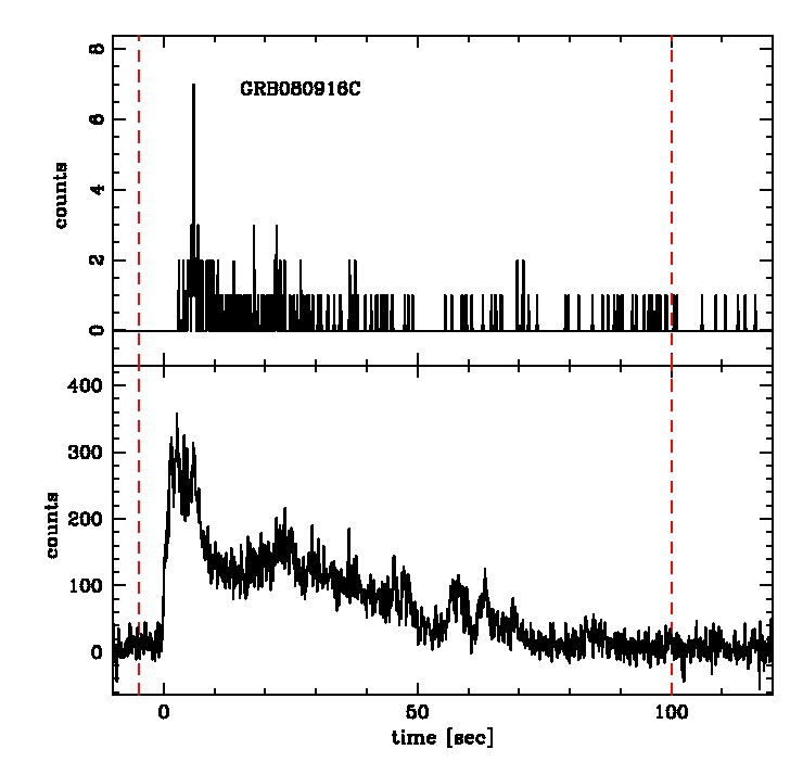
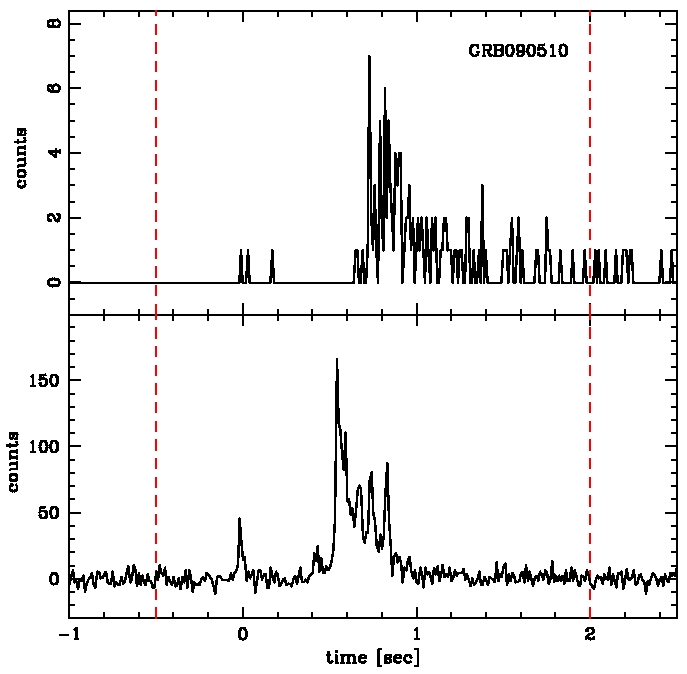
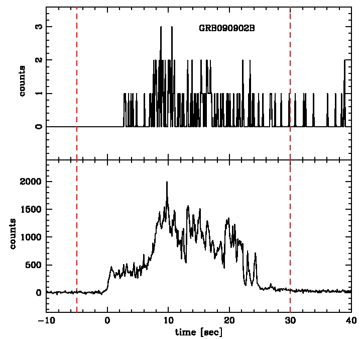
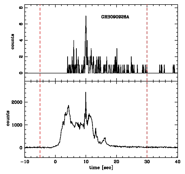
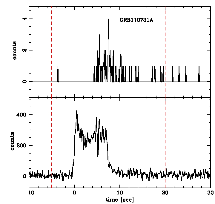
Figure 1: Light curves of the 5 GRBs. Top panels: background-subtracted 100 MeV - 300 GeV LAT light curves. Bottom panels: sum of the background-subtracted light curves from the two NaI detectors with the highest S/N. Vertical dashed lines show the light curve intervals used for the cross correlation analysis.

3 CCF method and results

In this section we focus on the continuous correlation function and consider the unbinned GBM and LAT light curves (see Sects. 2.1 and 2.2). Each curve consists of a time series containing individual photon events. Following the prescription described in Scargle (2010), we performed a 1D Voronoi tessellation of the signals; i.e., we transformed each curve into a succession of rectangles (one for each photon). The basis of each rectangle goes from half way back to the previous photon and ends half way forward to the subsequent photon. The height is fixed by requiring a unitary area for each rectangle. The advantage of this representation is that the light curves are now defined at each time and the delta-like discontinuities corresponding to the individual events are reduced to step discontinuities. However, we cannot straightforwardly subtract a background. For this reason, we preferred to consider each GBM NaI light curve separately. For each GRB, we performed the ordinary correlation function analysis (e.g., Papoulis, 1965, 1977) between the LAT and the GBM light curves in their Voronoi representation (see Scargle, 2010, and references therein). Because of poor number count statistics that mainly affects the LAT light curves, the Voronoi representation assumes low rates at each time. Therefore, the resulting GBM vs. LAT correlation function is similarly suppressed down to null or negligible values. The results of the correlation analysis are therefore inconclusive.

4 DCF method and results

The DCF at the lag $\tau$ is estimated by considering all the pairs that are separated in time by an amount between $\tau-\Delta\tau/2$ and $\tau+\Delta\tau/2$, where $\Delta\tau$ is a specific time binning of the DCF. Conversely, the CCF at the lag $\tau$ is obtained from all the pairs that are separated in time by exactly the amount $\tau$.

The choice of the time binning for the search of correlation between the two signals is dictated by the need to sample the possible time lag accurately (i.e., at least with $\sim$5 DCF points) and to have decent S/N in the estimate of the DCF in all time bins. In our case, the time lags we are testing are a few seconds ($\sim$0.1 s in the case of GRB090510). Therefore, they are significantly shorter than the duration of the GRB itself (Abdo et al., 2009a, b, c; Ackermann et al., 2011, 2013a).

We subtracted the averages from each of the background-subtracted LAT and GBM light curves and applied the DCF method (following Edelson & Krolik, 1988) to these light curves over the time intervals marked in Fig. 1. In particular, we weighed the DCF with the product of the rms dispersions around the averages of each of the background-subtracted light curves. We did not introduce other corrections to the method (White & Peterson, 1994), such as weighted averages or subtraction of individual errors from the light curves variances. This is because the noisy signal and the small number counts, especially for the LAT instrument, prevented us from estimating the uncertainties in the number counts robustly and, in turn, the corrections.

A DCF time bin of 1 sec was adopted for the long GRBs and 0.05 sec for GRB090510. This choice represents an optimal compromise between sufficient number count statistics for each DCF bin and a satisfactory sampling of the time lag between the two signals, as we verified a posteriori by inspecting the DCF. DCFs of our GRBs are reported in Fig. 2, with their individual one-sigma uncertainties. We verified that the DCFs do not significantly change if slightly different DCF time bins are adopted. The same holds if – for every GRB – either of the two background-subtracted GBM light curves corresponding to the two NaI detectors with the highest S/N, instead of the sum of them, is considered. All DCF curves exhibit a maximum at a formally positive time lag (except for GRB090902B), indicating that the LAT signal is possibly delayed with respect to the GBM signal.

Since the DCF method does not return any uncertainty on the time lag at which the correlation reaches its maximum, we estimate the location of the DCF maximum by fitting the DCF with a constant plus an asymmetric Gaussian function, $f(t)$, over a time interval centered on the peak:

$$f(t)=A+B\times\begin{cases}\exp\left[-\frac{1}{2}\left(\frac{t-\mu}{\Sigma_{r}}\right)^{2}\right]&{\rm if\hskip 5.69046ptt}\leavevmode\nobreak\ \geq\mu\\ \hskip 1.42271pt\\ \exp\left[-\frac{1}{2}\left(\frac{t-\mu}{\Sigma_{l}}\right)^{2}\right]&{\rm otherwise}\end{cases}.$$ (1)

This approach is similar to that of Zhang et al. (1999), although a symmetric Gaussian satisfied their purposes. It is a simplified and empirical assumption: there is no theoretical and observational reason to prefer one specific form for the function $f$. The Gaussian assumption provides both a rough estimate for the uncertainty on the time lag and a robust estimate of the time lag itself. They are given by the Gaussian dispersion and the lag at which the $f$-function reaches its maximum ($\mu$), respectively. We also estimate the formal error associated with the $\mu$ parameter according to the $\chi^{2}$ statistics. However, the $\Sigma_{r}$ and $\Sigma_{l}$ parameters are better estimators for the uncertainty associated with the time lag than the formal error associated with the $\mu$ parameter. This is because the $\Sigma_{r}$ and $\Sigma_{l}$ parameters represent the extent of the DCF spreading around its maximum. In fact, the width of the DCF maximum shows the range of time lags within which the correlation peak occurs. Conversely, the $\mu$ parameter error, estimated with the $\chi^{2}$ statistics, represents how well our model fits the data. Therefore, such an estimate is clearly model dependent and physically unrelated to the actual time lag uncertainty.

In Table 1 (Cols. 2 to 6) we report the best-fit parameters, along with the corresponding one-sigma formal errors obtained by the $\chi^{2}$ parameter marginalization (Cash, 1976). In Fig. 2 we plot the best-fit curves.

All DCFs exhibit clear peaks of correlation, while anti-correlation is excluded; i.e., no negative minimum is observed. The time lags of the correlations are positive, with the exception of GRB090926A, but they are never significantly different from zero at the 1-$\sigma$ level (see Cols. 3, 4, 5 in Table 1).

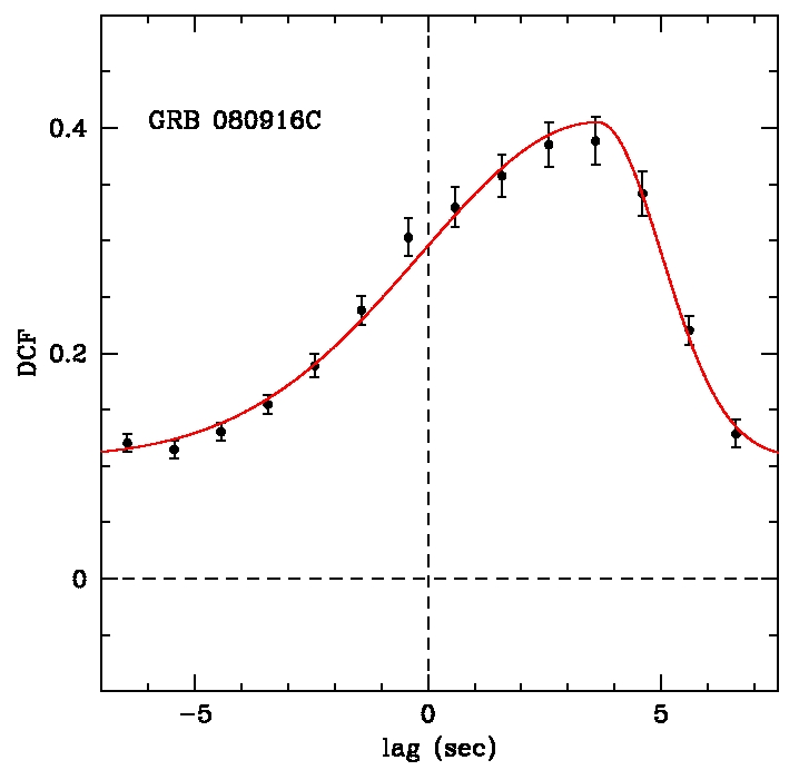
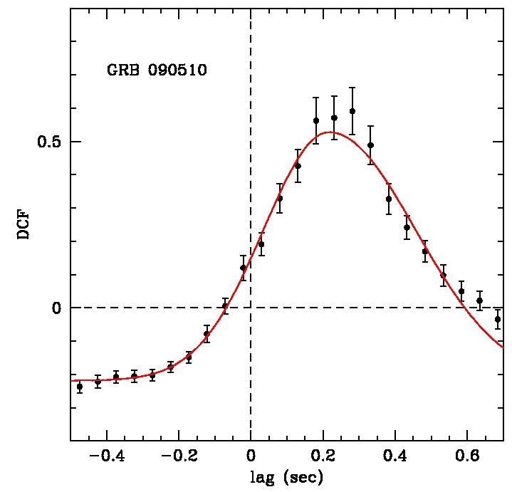
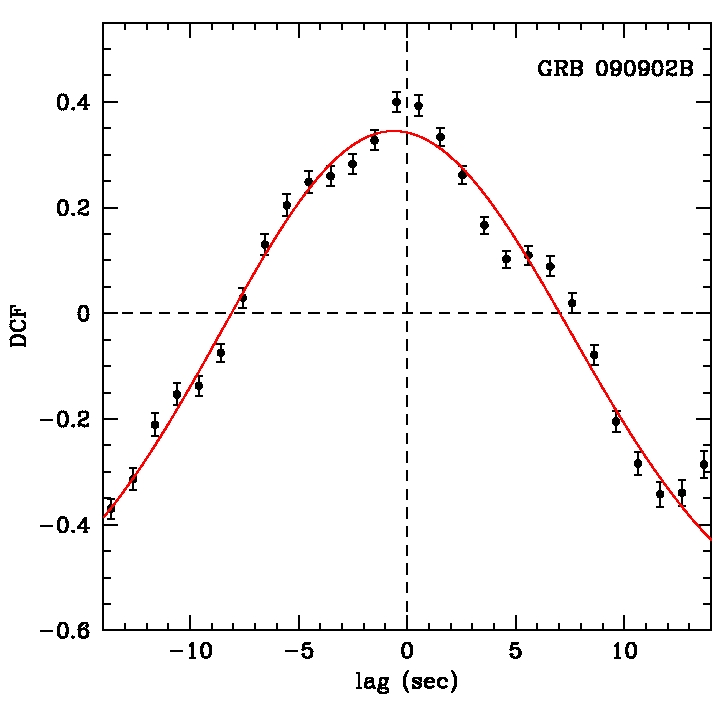
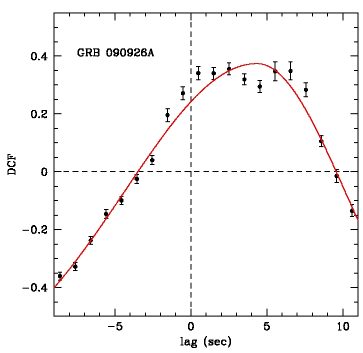
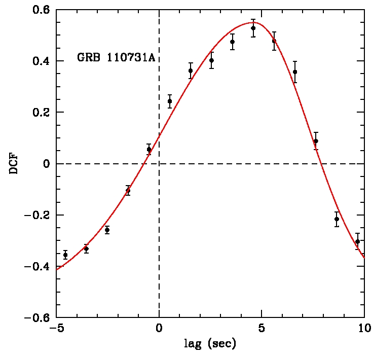
Figure 2: DCF curves, with individual 1-sigma uncertainties, between the LAT and GBM light curves of our 5 GRBs. Positive time lags suggest that the LAT is lagging the GBM signal. The solid red curve is the asymmetric Gaussian plus constant function that best fits the DCF peak.

Table 1: Best-fit parameters for the time lags between observed and simulated LAT and GBM light curves.

GRB	Aa	$\mu^{a}$ (s)	${\Sigma_{r}}^{a}$ (s)	${\Sigma_{l}}^{a}$ (s)	Ba	lagb (s)	lagc (s)	Td (s)	Ref.e
(1)	(2)	(3)	(4)	(5)	(6)	(7)	(8)	(9)	(10)
080916C	0.11$\pm$0.01	3.65$\pm$0.22	1.36$\pm$0.17	3.81$\pm$0.22	0.30$\pm$0.01	$3.79^{+0.26}_{-0.55}$	–	$\sim$3.6	1
090510	-0.22$\pm$0.02	0.22$\pm$0.02	0.24$\pm$0.02	0.18$\pm$0.02	0.75$\pm$0.02	$0.21^{+0.03}_{-0.06}$	–	$\sim$0.56	2
090902B	-0.62$\pm$0.09	-0.62$\pm$0.21	8.15$\pm$0.67	7.96$\pm$0.59	0.97$\pm$0.09	$-1.52^{+2.01}_{-1.00}$	$6.18^{+1.31}_{-0.80}$	$\sim$9.6	3
090926A	-0.75$\pm$0.09	4.36$\pm$0.26	5.78$\pm$0.36	8.70$\pm$0.72	1.12$\pm$0.09	$2.32^{+0.87}_{-0.94}$	$5.52^{+0.32}_{-0.64}$	$\sim$3.3	4
110731A	-0.47$\pm$0.03	4.62$\pm$0.17	2.71$\pm$0.16	4.45$\pm$0.24	0.98$\pm$0.03	$4.07^{+0.23}_{-0.18}$	–	$\sim$2.4	5
a Best fit parameters with formal 1-$\sigma$ errors for the constant plus asymmetric Gaussian function (Eq. 1). The
1-$\sigma$ asymmetric uncertainty on the $\mu$ parameter is given by the $\Sigma_{r}$ and $\Sigma_{l}$ parameters.
b Time lag and 1-$\sigma$ uncertainty derived from the maximum of the time lag distribution of simulated light curves.
c Time lag and 1-$\sigma$ uncertainty derived from the secondary maximum of the time lag distribution of simulated
light curves.
d Time lags based on the initial LAT delay, as reported in the literature.
e References for Col. 9: 1. Abdo et al. (2009a); 2. Abdo et al. (2009b); 3. Abdo et al. (2009c);
4. Ackermann et al. (2011); 5. Ackermann et al. (2013a).

5 Monte Carlo simulations and results

As stressed by Zhang et al. (1999), a constant plus Gaussian function, although representative of the peak position and the dispersion for the DCF, does not necessarily provide a statistically adequate fit. Furthermore, the presence of peaks in the correlation might be due to statistical fluctuations more than real time delays between the two signals. For these reasons we estimated the significance and the uncertainty of each time lag by means of Monte Carlo simulations, as prescribed in Peterson et al. (1998).

We apply the so-called “flux randomization” (FR) method (Peterson et al., 1998) to simulate $N$ light curves starting from the GBM and LAT observed, not background-subtracted, light curves. According to the FR procedure, we start from a certain light curve and produce a number $N$ of simulated signals that are drawn from a specific distribution (depending on the nature of the signal) whose average is equal to the observed light curve value, for each time. We applied the FR procedure to both the GBM and LAT light curves for each GRB. The simulated light curves are then correlated pairwise by means of the DCF, as described in Sect. 4. This provides a GBM vs. LAT time lag distribution that is used to derive the actual delay (if any is present) of the LAT emission with respect to the GBM emission.

We chose $N=10,000$ for each GRB in our sample. Given an observed light curve $\{F_{0},F_{1},...,F_{j},...\},$ we randomized the j-th number count at the time $t_{j}$ assuming a Poisson distribution around the average $\phi_{j}$, which is set equal to the flux $F_{j}$, if it is positive. Otherwise, we set $\phi_{j}$ equal to the background level estimated at the time $t_{j}$ for the given GRB and the considered detector. For GRB090926A we were not able to estimate an LAT background (see Sect. 2.2). Therefore, for this GRB alone, where $F_{j}=0$, we assume $\phi_{j}=\beta\times\Delta$t, where $\Delta$t is the bin of the LAT light curve, and $\beta$ is chosen to be 0.01 c/s and 0.1 c/s. These values are consistent with the LAT background estimated for the other GRBs in the sample. Then, for all GRBs, we subtract the background from each simulated light curve. Assuming Poisson uncertainties for the observed number counts only leads to small deviations from the more correct estimate that is generally used for small number counts, as is the case for LAT light curves (i.e., N$<$10, see, e.g., Gehrels, 1986).

For each GRB, the 2$\times N$ GBM NaI simulated light curves are pairwise summed in such a way that the two simulated curves in a given pair never come from the same NaI detector light curve and that each of the 2$\times N$ NaI simulated light curves belongs to one and only one pair.

Then, we have $N$ simulated LAT and $N$ simulated GBM background-subtracted light curves, which we compared pairwise with the DCF method, as in Sect. 4. We chose DCF time bins equal to those adopted for the correlation of the observed light curves: 1.0 sec for the long GRBs, 0.05 sec for the short GRB090510. As in Sect. 4, we limited the DCF analysis to the time intervals of the GBM and LAT light curves designated in Fig. 1.

We fit the $N$ DCFs obtained by cross-correlating the simulated GBM and LAT light curves with a constant plus asymmetric Gaussian function ($f(t)$, see Eq. 1). The fit is performed with the minimum-$\chi^{2}$ method. This is analogous to what was done in Sect. 4 for the DCF obtained by cross-correlating the observed light curves.

In Fig. 3 we report the resulting distributions of best-fit time lags. These distributions are fitted with an asymmetric Gaussian, since they are evidently asymmetric on either side of the maximum. In Table 1 (Col. 7) for each GRB we report the corresponding best fit parameters (i.e., the lag at which the Gaussian reaches its maximum; the reported uncertainties are the square roots of the two Gaussian variances). Concerning GRB090926A, we plot only the results corresponding to $\beta=$0.1 c/s, since we have verified that they are similar for $\beta=$0.01 c/s.

The time lags that are obtained according to this procedure are consistent with those derived from the observed DCFs (Col. 3). With the exception of GRB090902B, they are also compatible with those reported by the LAT team based on the initial delay of the LAT with respect to the GBM signal (Col. 9). However, since the uncertainties are smaller than those determined from the Gaussian fits of observed DCFs in Sect. 4, the time lags of GRBs 080916C, 090510A, and 110731A are significantly different from zero at the 3-$\sigma$ level.

In the case of GRBs 090902B and 090926A, the time lag distributions suggest that there are secondary maxima at $\sim$6 s (see Fig. 3 and Table 1, Col. 8). Close inspection of Fig. 2 shows that the presence of two maxima is also marginally seen in the DCF of the observed light curves. This is because a modest deviation from a clear single Gaussian fit occurs for both of these DCF: a shoulder (at about $\sim 5$ s) and two bumps (at $\sim$2.5 s and $\sim$6 s) are present in the DCF of GRB090902B and GRB090926A, respectively.

For both GRBs, the secondary maxima are consistent with the time lags reported by the LAT team (Table 1, Col. 9). However, by excluding those DCF fits that are significant at a $4\sigma$ level or lower, according to the $\chi^{2}$ statistics (i.e., by rejecting those fits with $\chi^{2}{\rm/dof}\gtrsim$3), these secondary maxima become much less significant (see Fig. 3).

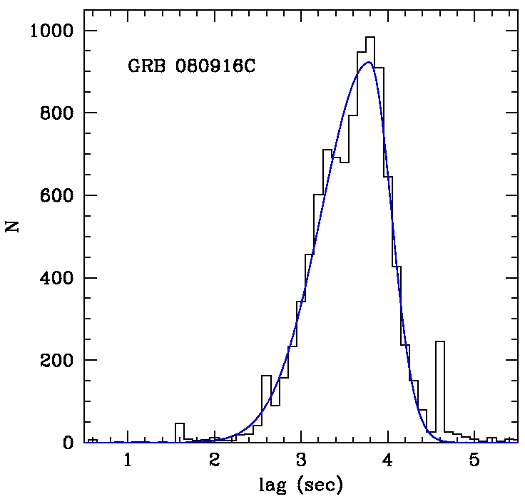
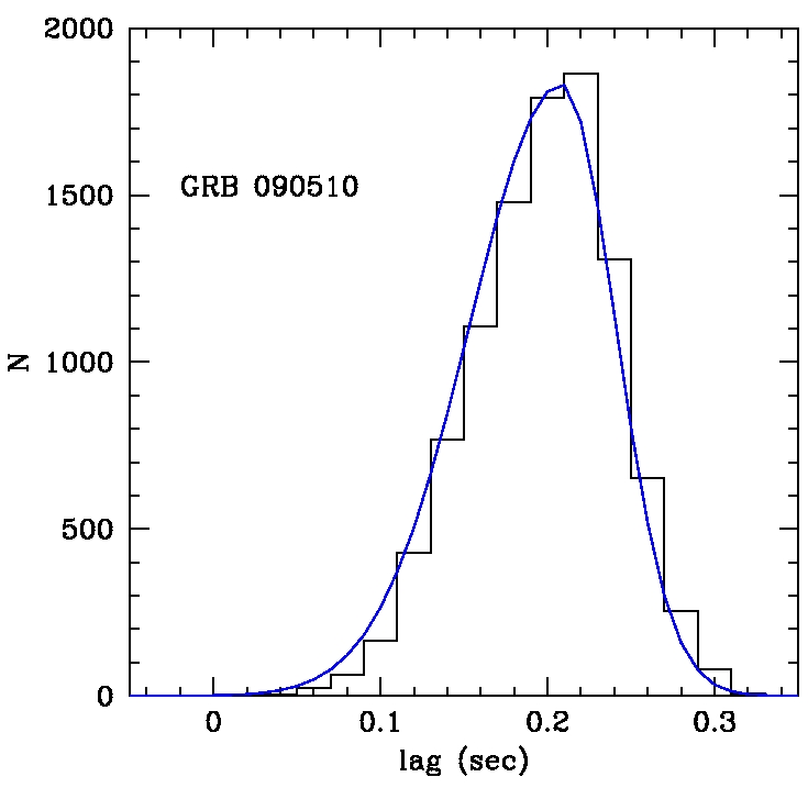
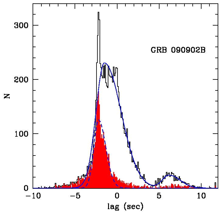
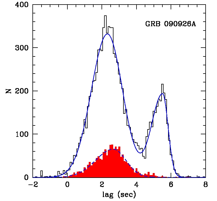
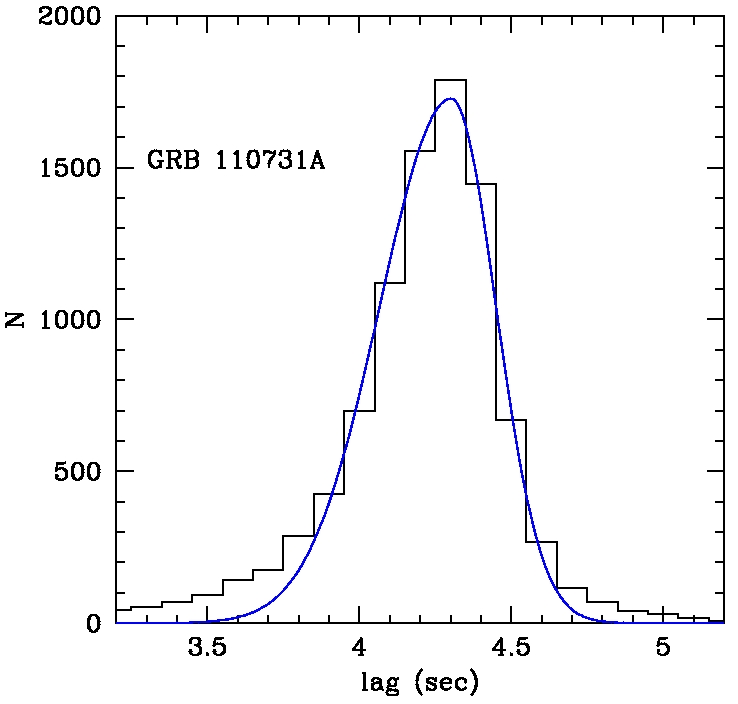
Figure 3: Time lag distributions (black histograms) obtained by cross-correlating the simulated GBM and LAT light curves. Positive time lags correspond to the LAT signal lagging the GBM signal. The asymmetric Gaussian fit is reported as a blue solid line. The red areas correspond to the distributions of time lags obtained considering those fits that are significant at a $4\sigma$ level or higher, according to the $\chi^{2}$ statistics (i.e., fits with $\chi^{2}/{\rm dof}\gtrsim$3 are rejected). The asymmetric Gaussian fit for the red areas is reported as a blue dashed line.

6 Conclusions

Motivated by the detection of time delays between the onset of LAT and GBM signals in Fermi-detected GRBs, we have adopted the DCF method to cross-correlate the LAT and GBM light curves of the five brightest LAT GRBs in the first Fermi LAT GRB catalog and thus to estimate the delay between the arrival times of MeV-GeV and $\sim$100-keV energy photons over the whole time evolution of the GRBs. We searched for delays both in the observed light curves and in light curves that were randomly generated via Monte Carlo simulations.

From the DCF of the observed light curves, we derived the time lags using a constant plus an asymmetric Gaussian approximation of the DCF maximum and determined the formal errors associated with a Gaussian fit (Table 1, Cols. 2-6). The reliability of these uncertainties depends on the correctness of the Gaussian approximation of the DCF profile around its maximum.

For each GRB, we also performed the individual DCFs of simulated light curves and estimated the associated time lags, analogously to what was done for the DCF obtained by using the observed light curves. This allowed us to independently estimate both the time lag and its uncertainty as the average and the square root of the variance of the Gaussian fit function, respectively (Table 1, Cols. 7 and 8). The estimates obtained by adopting the time lag distributions are more robust than those obtained by using the individual DCF that results from the observed light curves. This is because the estimates derived from the individual DCFs are based on a statistical approximation, rather than on a functional form description of the individual DCFs.

The time lags derived from the DCFs of the observed light curves are all formally consistent with zero, although they are mostly similar to those reported in the literature. This result is analogous to what is reported by Del Monte et al. (2011), who, using the cross-correlation approach, do not recover statistical significance for the time delay of $\sim$10 s observed between the start time of the AGILE MCAL and GRID light curves of GRB100724A.

When the simulated light curves are cross-correlated and the resulting time lag distributions are fitted with Gaussian functions, in three cases (i.e. GRBs 080916C, 090510A, 110731A) the best-fit time lags are significantly different from zero and compatible with those reported in the literature. For GRB090902B, the main time lag ($\sim$ -2 s) is formally very different from what has been previously reported (9.6 s, Abdo et al., 2009b), but not significantly different from zero. For GRB090926A, the main time lag (2.3 s) is consistent with the one reported by Ackermann et al. (2011), but again not significantly different from zero. However, GRBs 090902B and 090926A also have secondary maxima in their time lag distributions. For both GRBs they correspond to time lags that are significantly different from zero and similar to those previously reported in the literature. We note that the secondary maxima become less significant when only the satisfactory fits ($\chi^{2}{\rm/dof}\lesssim 3$) are retained. The reason may be that, since the fits corresponding to the secondary maxima generally have a more limited significance than those associated with the primary maxima, the DCF curves where they are more prominent have a complex morphology and are not well fit.

The presence of these secondary maxima suggests a complexity in the time behavior of the gamma-ray signals. While in general our results suggest that the cross-correlations are influenced by the observed initial delays between the LAT and GBM light curves, they also show other time scales and suggest that these delayed LAT signal onsets are probably due to intrinsic physics. A systematic cross-correlation analysis on a bigger sample than used here may set better constraints on the physical origin of the time delays.