Higher order quark-mesonic scattering processes and the phase structure of QCD

Abstract

We study the impact of higher order quark-meson scattering processes on the chiral phase structure of two-flavour QCD at finite temperature and quark density. Thermal, density and quantum fluctuations are included within a functional renormalisation group approach to the quark-meson model. We present results on the chiral phase boundary, the critical endpoint, and the curvature of the phase transition line at vanishing density.

I Introduction

The understanding of the formation and the properties of hadronic matter requires that of the phase structure of Quantum Chromodynamics (QCD). For fixed density the QCD vacuum changes drastically with decreasing temperature from a deconfined quark-gluon plasma phase with effective chiral symmetry to a hadronic phase with confined quarks and broken chiral symmetry. Future and running heavy-ion experiments e.g. at CERN, FAIR, BNL and JINR aim at probing this phase transition, especially also at high densities Braun-Munzinger et al. (2003).

The main challenge for theoretical studies of the QCD phase diagram lies in its non-perturbative nature, and the – related – dynamical change of relevant degrees of freedom. However, in the past decade rapid progress has been made in the first principle description of QCD at finite temperature and density, both with continuum methods, see e.g. Braun (2009); Braun et al. (2011); Pawlowski (2011); Herbst et al. (2013a); Fischer et al. (2011); Fischer and Luecker (2013); Fischer et al. (2013), and on the lattice, see e.g. Karsch (2002); Philipsen (2007); de Forcrand (2009); Sexty (2013). Within the continuum approach it has been worked-out in detail how low energy effective models are systematically embedded in first principle QCD, see Braun et al. (2011); Pawlowski (2011); Kondo (2010); Herbst et al. (2011, 2013b); Haas et al. (2013); Herbst et al. (2013a). It is a particular strength of such an approach that the necessary quantitative control over the matter and glue sector can be achieved separately, followed by a systematic combination of both sectors including their mutual back-reaction. This puts an even bigger emphasis on the systematic improvement of the corresponding low energy effective models of QCD. It not only furthers our understanding of the mechanisms underlying the pyhsics phenomena responsible for the phase structure of QCD but also is necessary for quantitatively describing the phase structure within a first principle continuum approach.

For small chemical potential the lightest hadronic states, the pions and the sigma-meson, drive the chiral dynamics in the vicinity of the phase boundary. Thus, in order to achieve quantitative control over the matter sector of QCD, and in particular the phase stucture, one has to accurately take into account the effects of mesonic fluctuations. The importance of such a procedure has been already observed in the context of higher order mesonic self-scatterings. These have been taken into account within low energy effective models in terms of full mesonic effective potential, for reviews see e.g. Berges et al. (2002); Schaefer and Wambach (2008); Braun (2012); von Smekal (2012). It is also well-known that a corresponding Taylor expansion converges well towards the results obtained with a full mesonic effective potential Papp et al. (2000). For a fully self-consistent expansion it is important to realise that quark–anti-quark multi-meson interactions have to be taken into account as well. Indeed, these terms contribute directly to the computation of the effective potential in the functional renormalisation group (FRG) approach.

Hence, in the present work, for the first time, we systematically also include higher order quark–anti-quark multi-meson interactions within the quark-meson (QM) model, and study their effect on the chiral phase structure of two-flavour QCD. In the QM model this amounts to a meson-field–dependent Yukawa coupling. The quantum, thermal, and density fluctuations are then taken into account by means of the FRG. This also allows us to consider the momentum-dependence of the propagators in terms of scale-dependent wave function renormalisations. Such effects are particularly relevant in the presence of massless excitations such as the pions close to a second order phase transition. The higher quark-meson interactions are included in a – convergent – Taylor expansion in the order of the mesonic fields. In total this leads to a significant extension of the local potential approximation of the quark meson model which has been used extensively to study the chiral phase transition of QCD, see e.g. Berges et al. (2002); Schaefer and Wambach (2008, 2005).

We present results on the chiral phase boundary in the $T$-$\mu$ plane, including the critical endpoint and the curvature of the phase boundary. We also compare different definitions of the phase boundary. This is particularly important in the region of the phase diagram where the system undergoes a crossover transition and the exact location of the phase boundary is not uniquely defined. We find that the inclusion of the higher order couplings lead to quantitatively significant changes in the phase structure. An intriguing observation is the rapid convergence of our results if the orders of meson-meson and quark-meson couplings are increased.

Our present findings are fully in the spirit of the systematic embedding of the low energy effective models in first principle QCD. They constitute significants steps towards quantitative precision in terms of convergence of a self-consistent truncation for the matter sector of QCD.

The present work is organised as follows: In section II we briefly introduce the quark-meson model in the context of full QCD, including the higher order quark-meson scattering processes in terms of an effective meson potential, a field-dependent Yukawa coupling and quark and meson wave function renormalisations. Section III summarises the renormalisation group approach and provides some details about the resulting flow equations of our model. Our results are presented in section IV, where we demonstrate the convergence of our expansion scheme and discuss the chiral phase structure at finite temperature and quark chemical potential including the critical endpoint and the curvature at vanishing chemical potential. Conclusions are given in section V. A discussion of the expansion scheme as well as some details on the flow equations can be found in the Appendices.

II Quark-Meson model

In the present work we concentrate on two-flavour QCD by employing a quark-meson model as a low energy effective model for QCD. As already mentioned in the introduction, it is by now well understood how such low-energy effective models are embedded in first-principle QCD within functional methods. The key concept behind this embedding in full QCD the the consistent treatment of the dynamical change of the relevant degrees of freedom. Starting from the high temperature/large cut-off scale quark-gluon phase, the system is dynamically driven towards the low temperature/small cut-off scale hadronic phase, where chiral symmetry breaking is triggered by the increasing gauge coupling.

This transition from a description in terms of quarks and gluons to a hadronic description is achieved by dynamical hadronisation Gies:2001nw; Gies:2002hq; Pawlowski (2007); Floerchinger:2009uf. Furthermore, while some hadronic degrees of freedom get dynamical at the hadronisation scale $\Lambda\!\approx\!1\,\text{GeV}$, the quark and gluon degrees of freedom decouple. This structure is very apparent in the Landau gauge, where the gluon propagator is infrared gapped, the gapping being directly related to the QCD mass gap, see e.g. Fischer:2008uz; Maas:2011se. Hence, the gluons can be integrated out first, leading to an effective theory with quarks and hadrons in a gluonic background potential, such as Polyakov-loop enhanced low-energy models.

This setting entails that first-principle QCD flows can be employed to provide initial parameters and further glue input, such as background potentials, for model calculations, thereby systematically removing ambiguities in these models. In particular, no double counting of degrees of freedom is present in quark-meson models in this context: the initial parameters of the low-energy theory are fixed uniquely by the first-principle QCD flows, and an unambiguous projection procedure for the flows of all couplings is given by a complete orthogonal set of projection operators which is also fixed uniquely by the relation to first-principle QCD. Such a procedure resolves for example, amongst other ambiguities, the well-known Fiertz ambiguity, see e.g. Braun (2012). This picture has successfully been applied to first-principle QCD at finite temperature and density, Braun et al. (2011); Pawlowski (2011), as well as to low energy effective models Herbst et al. (2011, 2013b); Haas et al. (2013), where quantitative agreement of QCD thermodynamics with lattice QCD is achieved Herbst et al. (2013a).

Here, our focus is on the chiral dynamics of QCD at energy scales $k\!\leq\!700\,\text{MeV}$. In the present work, dynamical hadronisation is not taken into account. We want to emphasise, however, that this plays a quantitative important role for large cutoff scales, where gluon-induced fermionic self-interactions in the chirally symmetric phase need to be taken into account properly. Since we start the RG-flow of our model at a scale $\Lambda\!=\!700\,\text{MeV}$, where composite degrees of freedom have already formed, dynamical hadronisation would only lead to very minor quantitative corrections. We have explicitly checked this statement for simpler QM models. We have also neglected the gluonic background which leads to a quantitative change of the phase boundary. This will be discussed elsewhere.

II.1 Low energy effective action

For an effective description of the low energy matter sector of QCD at not too high densities, a model based solely on quarks and the lightest meson is a good approximation. The ultraviolet cut-off scale $\Lambda$ of such a description, as already mentioned above, relates to the scale where the pure glue sector of QCD decouples and the fluctuations of the lightest mesons and constituent quarks dominate the dynamics. Here we consider $N_{\text{f}}=2$ degenerate quark flavours with pseudo-scalar pions $\vec{\pi}$ and the scalar sigma meson as the dominant mesonic degrees of freedom for not too large chemical potential at $\Lambda\approx 1$ GeV. At this scale the low energy effective action $\Gamma_{\Lambda}$ is approximated by that of the quark-meson model.

As described in the previous section, for momentum scales $k\lesssim\Lambda$, we take into account the scale-dependent dressing of the propagators and higher mesonic– as well as quark-meson–interactions. The corresponding scale-dependent effective action reads

$$\Gamma_{k} = \int_{x}\Bigl{\{}iZ_{\psi,k}(\rho)\bar{\psi}(\gamma_{\mu}\partial_{\mu}+\gamma_{0}\mu)\psi+\frac{1}{2}Z_{\phi,k}(\rho)(\partial_{\mu}\phi)^{2}\Bigr{.}$$ (1)

$$\Bigl{.}+V_{k}(\rho)-c\sigma+h_{k}(\rho)\bar{\psi}(\gamma_{5}\vec{\tau}\vec{\pi}+i\sigma)\psi\Bigr{\}}\,,$$

with the meson fields in the $O(4)$ representation, $\phi=(\vec{\pi},\sigma)$, and

$$\rho=\frac{1}{2}\phi^{2}=\frac{1}{2}(\vec{\pi}^{2}+\sigma^{2})\,.$$ (2)

In (1) we used the abbreviation $\int_{x}=\int_{0}^{1/T}dx_{0}\int d^{3}x$. The quark fields $\psi$ are two flavour Dirac-spinors and $\mu$ is the quark chemical potential. For $N_{\text{f}}=2$ the chiral symmetry $SU(N_{\text{f}})_{L}\otimes SU(N_{\text{f}})_{R}$ is isomorphic to $SO(4)$, hence the $O(4)$-symmetry of the scalar effective potential $V_{k}(\rho)$. Quarks and mesons are coupled via a meson field-dependent Yukawa coupling $h_{k}(\rho)$. $\vec{\tau}$ are the Pauli matrices.

This model captures spontaneous chiral symmetry breaking $SU(N_{\text{f}})_{L}\otimes SU(N_{\text{f}})_{R}\rightarrow SU(N_{\text{f}})_{V}$. The expectation value of the sigma meson serves as order parameter for the chiral phase transition and the three pions are Goldstone bosons of the spontaneous breaking of the axial $SU(2)_{A}$. In the presence of explicit symmetry breaking, introduced by the linear breaking term $-c\sigma$, the pions are not massless but rather pseudo-Goldstone bosons with finite mass and the chiral second order transition turns into a crossover.

The inverse quark and meson propagators are dressed with wave function renormalisations $Z_{\psi,k}(\rho)$ and $Z_{\phi,k}(\rho)$. Note that at finite temperature there are in general two different wave function renormalisations quarks and mesons, one perpendicular, $Z=Z^{\perp}$, and one parallel to the heat bath, $Z^{\|}$. In the present work we only compute the perpendicular one and identify $Z^{\|}=Z^{\perp}$. Moreover, we expect a weak dependence of the $Z$’s on the meson field $\rho$ and hence we drop all terms proportional to $\partial_{\rho}Z(\rho)$. This approximation is discussed in section III.3. The explicit breaking of $O(4)$-symmetry in the meson-sector of our model through the linear term $-c\sigma$ is related to a finite current quark mass $m_{q}^{c}$ via the relation

$$m_{q}^{c}=\frac{h_{\Lambda}}{\lambda_{1,\Lambda}}c\,,$$ (3)

where $\lambda_{1,\Lambda}$ is the squared meson mass in the UV, see (7).

II.2 Higher order mesonic scattering

The present approximation includes field-dependent wave function renormalisations $Z_{k}(\rho)$ for quarks and mesons, a full effective potential $V_{k}(\rho)$, and a field-dependent Yukawa-coupling $h_{k}(\rho)$. We implement higher order mesonic scattering processes via a systematic expansion in $n$-point functions $\Gamma^{(n)}$ of the effective action (1).

We first discuss the wave function renormalisations. The $\rho$-dependence of the mesonic wave function renormalisation contains momentum-dependent meson self-interactions while that of the quarks contains momentum-dependent scattering of a quark–anti-quark pair with mesons. Note that both processes vanish at vanishing momenta. The wave function renormalisations can be expanded about a temperature and chemical potential dependent and potentially scale-dependent expansion point $\kappa_{k}(T,\mu)$, to wit

$$Z_{k}(\rho)=\sum_{n=0}^{N_{Z}}\frac{Z_{n,k}}{n!}\left(\rho-\kappa_{k}(T,\mu)\right)^{n}\,.$$ (4)

However, we expect a rather mild dependence of the wave function renormalisation on the meson field, leading to

$$\partial_{\rho}Z_{k}(\rho)\approx 0\,.$$ (5)

The quantitative reliability of this hypothesis is tested in Appendix A, see in particular Fig. 11. Eq. (5) implies that locally (about a given expansion point $\kappa_{k}$) we can use

$$Z_{k}=Z_{0,k}\,.$$ (6)

Still, for the computation of observables the wave function renormalisation has to be determined at the expectation value $\rho_{0}$ of the mesonic field which does not necessarily agree with the expansion point $\kappa_{k=0}$. It is here where the field dependence of the $Z$’s play a r$\hat{\rm o}$le.

Meson self-interactions are contained in the effective potential $V_{k}(\rho)$. As for the wave function renormalisations we expand the effective potential in powers of $\rho$ about an expansion point $\kappa_{k}(T,\mu)$, to wit

$$V_{k}(\rho)=\sum_{n=1}^{N_{V}}\frac{\lambda_{n,k}}{n!}\bigl{(}\rho-\kappa_{k}\bigr{)}^{n}\,.$$ (7)

In (7) we have dropped all $T,\mu$-dependence for the sake of brevity. Eq. (7) captures a chiral crossover and a second order transition for $N_{V}\geq 2$. A first order transition requires at least $N_{V}\geq 3$. The effect of higher order mesonic self-interactions on the matter sector of QCD can be systematically studied by increasing the order of the expansion $N_{V}$.

It is convenient to rewrite the effective action in terms of the renormalised fields

$$\bar{\phi}=Z_{\phi,k}^{1/2}\,\phi\,,\qquad{\rm and}\qquad\bar{\rho}=Z_{\phi,k}\,\rho\,,$$ (8)

where the wave function renormalisations are locally constant in the present approximation. For the effective potential $\bar{V}(\bar{\rho})=V(\rho)$ this implies

$$\bar{V}_{k}(\bar{\rho})=\sum_{n=1}^{N_{V}}\frac{\bar{\lambda}_{n,k}}{n!}\bigl{(}\bar{\rho}-\bar{\kappa}_{k}\bigr{)}^{n}.$$ (9)

with

$$\bar{\lambda}_{n,k}=\frac{\lambda_{n,k}}{Z_{\phi,k}^{n}}\,,\qquad{\rm and}\qquad\bar{\kappa}_{k}=Z_{\phi,k}\,\kappa_{k}\,.$$ (10)

The $\bar{\rho}$-derivatives of the effective potential, $\partial_{\bar{\rho}}^{n}\bar{V}$, and that of the effective action allow for a direct physical interpretation as they are RG-invariant. The linear term in (1) reads in the new fields

$$c\sigma=\bar{c}_{k}\bar{\sigma}\,,\qquad{\rm with}\qquad\bar{c}_{k}=\frac{c}{Z_{\phi,k}^{1/2}}\,.$$ (11)

Quark–multi-meson interactions are taken into account in (1) by the coupling of two quarks and a meson with a $\rho$-dependent Yukawa coupling $h_{k}(\rho)$. Analogous to the effective potential, we also expand the Yukawa coupling in a $O(4)$-symmetric manner in powers of $(\rho-\kappa_{k})$,

$$h_{k}(\rho)=\sum_{n=0}^{N_{h}}\frac{h_{n,k}}{n!}\bigl{(}\rho-\kappa_{k}\bigr{)}^{n}\,.$$ (12)

$N_{h}=0$ amounts to the standard Yukawa interaction which couples a quark–anti-quark pair and a meson. By increasing $N_{h}$ the interaction between a quark–anti-quark pair and $(2N_{h}+1)$ mesons can be taken into account. The renormalised analogue of (12) reads

$$\bar{h}_{k}(\bar{\rho})=\frac{h_{k}(\rho)}{Z_{\psi,k}Z_{\phi,k}^{1/2}}=\sum_{n=0}^{N_{h}}\frac{\bar{h}_{n,k}}{n!}\bigl{(}\bar{\rho}-\bar{\kappa}_{k}\bigr{)}^{n}\,,$$ (13)

with RG-invariant expansion coefficients

$$\bar{h}_{n,k}=\frac{h_{n,k}}{Z_{\psi,k}Z_{\phi,k}^{(2n+1)/2}}\,.$$ (14)

The convergence of these expansions implies that the higher order couplings get increasingly irrelevant with increasing order of the meson field, see section IV.2. A more detailed analysis of the present expansion scheme is deferred to Appendix A. Here we only note that we choose a scale independent expansion point $\kappa$.

III Fluctuations

In the present work we include quantum, thermal and density fluctuations with the functional renormalisation group (FRG). In addition to its application to QCD, see Litim and Pawlowski (1998); Pawlowski (2007); Gies (2012); Pawlowski (2011); Rosten (2012) and corresponding low enegry effective models Berges et al. (2002); Schaefer and Wambach (2008); Braun (2012); von Smekal (2012), the FRG has been used successfully in a variety of physical problems ranging from ultracold atoms and condensed matter physics Delamotte (2012); Metzner et al. (2011); Boettcher et al. (2012); Braun (2012) to quantum gravity Niedermaier and Reuter (2006); Codello et al. (2009); Litim (2011); Reuter and Saueressig (2012).

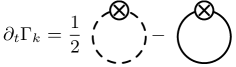
Figure 1: Diagrammatic representation of the flow equation for the matter sector of QCD. The dashed line represents the full meson propagator, the solid line the full quark propagator and the crossed circle depicts the regulator insertion.

The idea is to start with the effective action $\Gamma_{\Lambda}$ given in (1) at the initial scale $k=\Lambda$ and to successively include quantum fluctuations by integrating out momentum shells down to an infrared-cutoff scale $k$. By lowering $k$ we resolve the macroscopic properties of the system and eventually arrive at the full quantum effective action $\Gamma$ at $k=0$. This evolution of $\Gamma_{k}$ is governed by the Wetterich equation Wetterich (1993). For the quark-meson model it reads,

$$\begin{split}\partial_{t}\Gamma_{k}[\phi,\psi,\bar{\psi}]=&\frac{1}{2}\text{Tr}\!\left[\left(\frac{1}{\Gamma_{k}^{(2)}[\phi,\psi,\bar{\psi}]+R_{k}}\right)_{\phi\phi}\partial_{t}R_{k}^{\phi}\right]\\ &-\text{Tr}\!\left[\left(\frac{1}{\Gamma_{k}^{(2)}[\phi,\psi,\bar{\psi}]+R_{k}}\right)_{\psi\bar{\psi}}\partial_{t}R_{k}^{\psi}\right]\,,\end{split}$$ (15)

where $\partial_{t}$ is the total derivative with respect to the RG-time $t=\ln(k/\Lambda)$. The traces sum over the corresponding discrete and continuous indices including momenta and species of fields. $\Gamma_{k}^{(2)}[\phi,\psi,\bar{\psi}]$ is the matrix of second functional derivatives of $\Gamma_{k}$ with respect to the fields. The indices $\phi\phi$ and $\psi\bar{\psi}$ indicate the components in field space. In this notation the regulator $R_{k}$ is also a matrix in field space, where $R_{k}^{\phi}$ and $R_{k}^{\psi}$ are the entries corresponding to the meson and quark regulators respectively. The flow equation has a simple diagrammatic representation, see Fig. 1.

The specific regulators used in the present work are three-dimensional Litim regulators and are specified in (55) in Appendix B. They are proportional to the wave function renormalisations $Z_{\phi},Z_{\psi}$ and hence are RG-adapted, Pawlowski (2001, 2007); Gies (2002). As a consequence of this choice the $Z$’s completely drop out of the flows and only the anomalous dimensions survive. Note that this only holds true within the locally constant approximation for the wave function renormalisation. It also implies that our regulators depend on the expansion point. Note also that fully field-dependent wave function renormalisations $Z(\rho)$ cannot be introduced to the regulators without modifying the flow equation, see Pawlowski (2007). Such a flow will be considered elsewhere. The regulators suppress modes with momenta $p^{2}\lesssim k^{2}$ and thus implement the successive inclusion of fluctuations on ever-lower energy scales down to the scale $k$.

On the one hand such an approximation to the full QCD-flow is only satisfactory in the low energy regime of QCD at scales $k\lesssim 1$ GeV and k should be chosen as small as possible. On the other hand the initial cut-off scale $\Lambda$ has to be far bigger than any other physical scale under investigation, i.e. $T$, $\mu$ and the physical masses. In the present work we shall adopt $\Lambda=700\,\text{MeV}$. Note that $\Lambda$ receives a physical meaning in this context since it is directly related to the scale where hadrons form.

It is left to project the flow equation (15) for the effective action on the scale- and field-dependent parameters of the effective action defined in (1):

III.1 Effective potential

The flow equation of the effective potential $V_{k}(\rho)-c\sigma$ is obtained by evaluating (15) for constant meson fields, $\phi(x)\rightarrow\phi$, and vanishing quark fields. For these field configurations the effective action reduces to $\Gamma_{k}=\text{Vol}_{4}^{-1}\left(\bar{V}_{k}(\bar{\rho})-\bar{c}_{k}\bar{\sigma}\right)$, see (1). Note that the explicit symmetry breaking term is linear in the meson field, and hence is nothing but a source term. The right hand side of the flow equation (15) only involves second derivatives w.r.t. the fields. Thus, the explicit symmetry breaking term does not appear on the right hand side of the flow equation, which only depends on symmetric terms. Moreover the flow equation (15) is derived with cut-off–independent source terms, which implies $\partial_{t}c=0$. With (11) this leads to

$$\partial_{t}\bar{c}_{k}=\frac{1}{2}\eta_{\phi,k}\,\bar{c}_{k}\,,$$ (16)

with the (perpendicular) meson anomalous dimension

$$\eta_{\phi,k}=-\frac{\partial_{t}Z_{\phi,k}}{Z_{\phi,k}}\,.$$ (17)

This has the remarkable consequence, that in terms of fluctuations the theory is effectively evaluated in the chiral limit. Hence, this also applies to the effective potential $V_{k}$. The explicit $O(4)$ symmetry breaking introduced via the linear term $c\,\sigma$ simply entails that the vacuum expectation value of the fields is shifted relative to that in the chiral limit. In other words, the physical observables that can be derived from $V_{k}$ and its derivatives are evaluated away from the minimum of $V_{k}$. Note also in this context that we could choose any $k$-dependence for $c_{k}$, only the value at $k=0$ is fixed by the physical quark masses. The flow for $\bar{V}_{k}(\bar{\rho})=V_{k}(\rho)$ reads

$$\begin{split}\left.\partial_{t}\right|_{\rho}\bar{V}_{k}(\bar{\rho})=&\frac{k^{4}}{4\pi^{2}}\left\{\left[(N_{\text{f}}^{2}-1)\,l_{0}^{(B,4)}(\bar{m}_{\pi,k}^{2},\eta_{\phi,k};T)\right.\right.\\ &\left.+l_{0}^{(B,4)}(\bar{m}_{\sigma,k}^{2},\eta_{\phi,k};T)\right]\\ &\left.-4N_{c}N_{f}\,l_{0}^{(F,4)}(\bar{m}_{\psi,k}^{2},\eta_{\psi,k};T,\mu)\right\}\,,\end{split}$$ (18)

with the (perpendicular) quark anomalous dimension,

$$\eta_{\psi,k}=-\frac{\partial_{t}Z_{\psi,k}}{Z_{\psi,k}}\,.$$ (19)

Eq. (18) is nothing but the flow equation $\partial_{t}V(\rho)$. The threshold functions $l_{0}^{B/F,4}$ are defined in Appendix B, and depend on the field-dependent dimensionless renormalised masses

$$\bar{m}_{\pi,k}^{2}=\frac{\partial_{\bar{\rho}}\bar{V}_{k}}{k^{2}}\,,\qquad\qquad\bar{m}_{\sigma,k}^{2}=\frac{\partial_{\bar{\rho}}\bar{V}_{k}+2\rho\,\partial^{2}_{\bar{\rho}}\bar{V}_{k}}{k^{2}}\,,$$ (20)

and

$$\bar{m}_{\psi,k}^{2}=\frac{2\bar{h}_{k}(\bar{\rho})^{2}\bar{\rho}}{k^{2}}\,.$$ (21)

The first and second lines in (18) are the pion and the sigma meson contributions respectively. The third line in (18) is the quark contribution, where $2N_{c}N_{f}$ is the number of internal quark degrees of freedom. The additional factor $-2$ is generic for fermionic loops.

The flow of the renormalised couplings $\bar{\lambda}_{n}$ is derived from (9) as ($n\geq 1$),

$$\begin{split}&\left.\partial^{n}_{\bar{\rho}}\left.\partial_{t}\right|_{\rho}\bar{V}_{k}(\bar{\rho})\right|_{\bar{\rho}=\bar{\kappa}_{k}}\\ &\qquad=\left(\partial_{t}-n\,\eta_{\phi,k}\right)\bar{\lambda}_{n,k}-\bar{\lambda}_{n+1,k}\,\left(\partial_{t}+\eta_{\phi,k}\right)\bar{\kappa}_{k}\,.\end{split}$$ (22)

where we have used that (8) implies

$$\partial_{t}\bar{\rho}=-\eta_{\phi,k}\bar{\rho}\,.$$ (23)

We have computed the scale derivative at fixed $\rho$ as we want to connect (22) to (18): the left hand side of (22) is the $n$th derivative w.r.t. $\bar{\rho}$ of the flow equation (18). The relative sign for the $\eta_{\phi,k}$-terms in the second line of (22) reflects the factor $1/Z_{\phi,k}$ in the renormalised couplings in comparison to the factor $Z_{\phi,k}$ in the expansion point $\bar{\kappa}$.

The equations (22) with (18) provide a tower of coupled differential equations for higher order mesonic correlators and therefore include meson-meson scattering up to order $2N_{V}$ into our model. We now use the freedom of choosing an expansion point $\bar{\kappa}$ in order to improve the convergence property of the Taylor expansion. To that end we note that an expansion about fixed $\bar{\rho}=\bar{\kappa}$ with $\partial_{t}\bar{\kappa}=0$ keeps a term proportional to $\bar{\lambda}_{n+1}$ on the right hand side of (22). Such a linear dependence of the flow of $\bar{\lambda}_{n}$ potentially destabilises the expansion as the $\bar{\lambda}_{n+1}$ grow rapidly with $n$ even though their relevance for the potential decreases rapidly. This is indeed the case as we have checked within an explicit numerical computation. Note that this argument also applies to an expansion about the scale dependent minimum of the effective potential $\bar{\rho}_{0,k}$.

In turn, the linear $\bar{\lambda}_{n+1}$-contribution vanishes precisely for

$$\partial_{t}\bar{\kappa}_{k}=-\eta_{\phi,k}\bar{\kappa}_{k}\,,\qquad\to\qquad\partial_{t}\kappa=0\,.$$ (24)

that is a scale-independent bare expansion point. We emphasise that it is only the expansion about a fixed bare field value that removes the destabilising back-coupling of the higher order couplings. Therefore, it is the preferred expansion point in terms of convergence of the expansion. An explicit numerical check indeed reveals the rapid convergence of such an expansion, see Section IV.2. However, we have also checked that both expansions convergence to the same results.

We close this Section with a discussion of possible order parameters. For a large region of the phase diagram the chiral transition is a cross-over. This only allows for the definition of a pseudo-critical temperature which is not unique. All possible definitions of pseudo order parameters have the property that they provide order parameters in the chiral limit where the cross-over turns into a second order phase transition. Here we discuss several order parameters. The variance of the pseudo-critical temperatures provide a measure for the width of the cross-over.

A simple order parameter of the chiral transition (in the chiral limit) is given by the vacuum expectation value $\bar{\sigma}_{0,k}$ at vanishing cut-off. It also determines the pion decay constant, $f_{\pi}=\bar{\sigma}_{0,k=0}$. The expectation value $\bar{\sigma}_{0,k}$ is obtained from

$$\Bigl{.}\partial_{\bar{\rho}}\left[\bar{V}_{k}(\bar{\rho})-\bar{c}_{k}\bar{\sigma}\right]\Bigr{|}_{\bar{\rho}=\bar{\rho}_{0,k}}=0,$$ (25)

where $\bar{\rho}_{0,k}=\frac{1}{2}\bar{\sigma}_{0,k}^{2}$ is the quadratic order parameter. Physical observables such as the pion decay constant and the masses are then defined at vanishing cut-off scale $k=0$ and $\bar{\rho}=\bar{\rho}_{0,\text{IR}}$.

The position of the peak of the chiral susceptibility is an alternative definition of the phase transition temperature. The chiral susceptibility measures the strength of chiral fluctuations. Hence it is, independent of its use for constructing an order parameter, an interesting observable. It is defined as the response of the chiral condensate $\left\langle\bar{\psi}\psi\right\rangle$ to variations of the current quark mass $m_{q}^{c}$,

$$\chi_{\bar{q}q}=\frac{\partial\!\left\langle\bar{\psi}\psi\right\rangle}{\partial\bar{m}_{q}^{c}}.$$ (26)

Within our model the scale dependent chiral condensate is given by Ellwanger and Wetterich (1994); Berges et al. (1999)

$$\left\langle\bar{\psi}\psi\right\rangle_{k}=-\frac{1}{h_{\Lambda}}\left(\lambda_{1,\Lambda}\sigma_{0,k}-c\right).$$ (27)

The current quark mass is given by (3). Combining (27) and (3) yields the following relation:

$$\frac{\partial\sigma_{0,\text{IR}}}{\partial c}=-\frac{h_{\Lambda}^{2}}{\lambda_{1,\Lambda}^{2}}\chi_{\bar{q}q}+\frac{1}{\lambda_{1,\Lambda}}.$$ (28)

Note that for (27) to hold with high accuracy, we need to require that the expansion point $\kappa$ is very close to the physical point $\rho_{0,k}$. This is indeed the case for our choice of the expansion point, see (45).

We can rewrite (28) by virtue of the implicit function theorem since the relation between $\sigma_{0,k}$ and $c$ is implicitly given by (25). This yields:

$$\frac{\partial\sigma_{0,k}}{\partial c}=\Bigl{(}V^{\prime}_{k}(\rho_{0,k})+2\rho_{0,k}V^{\prime\prime}_{k}(\rho_{0,k})\Bigr{)}^{-1}=\frac{1}{m_{\sigma,k}^{2}}.$$ (29)

Thus, in practice we can compute the sigma meson mass and readily extract the chiral susceptibility for given initial parameters $\lambda_{1,\Lambda},\,h_{\Lambda}$.

III.2 Yukawa coupling

The scalar part of the Yukawa-term has been introduced in (1) as a $\phi$-dependent fermionic mass term with mass $h(\rho)\sigma$. This definition also entails that in leading order in $\rho$ the sigma field has been introduced as a field for the composite operator $\bar{\psi}\psi$. Accordingly we evaluate the flow of the fermionic two-point function at the minimal fermionic momentum $p_{\rm low}$ and constant mesonic fields, leading to

$$\begin{split}\partial_{t}h_{k}(\rho)=&-\frac{1}{\sigma}\frac{i}{4N_{\text{c}}N_{\text{f}}}\\ &\times\text{Re}\left[\lim_{p\rightarrow p_{\text{low}}}\text{Tr}\left.\left(\frac{\delta^{2}\partial_{t}\Gamma_{k}}{\delta\psi(-p)\delta\bar{\psi}(p)}\right)\right|_{\rho(x)=\rho}\right],\end{split}$$ (30)

where the trace in (30) sums over all internal indices. Note that (30) is well-defined even in the limit $\sigma\to 0$. The diagrammatic representation of this equation is depicted in Fig. 2.

In (30) we have set the external spatial momenta to zero and the external Matsubara frequencies to their lowest mode, $p_{\text{low}}=(\pi T,\vec{0}\,)$ for quarks. Implicitly we also use $p_{\text{low}}=(0,\vec{0}\,)$ for mesons as we evaluate the Yukawa coupling for constant mesonic fields. For finite quark chemical potential this procedure yields a manifestly complex valued flow on the right hand side of (30). This simply reflects the dependence of the two-point function on $p_{0}-i\mu$ and hence the momentum-dependence of the Yukawa coupling $h$: Evaluated at constant mesonic fields the Yukawa coupling is a function of $\rho$, $(p_{0}-i\mu)^{2}$, $\vec{p}^{2}$ and $\mu$ with real expansion coefficients: $h(p_{0}-i\mu)^{*}=h(p_{0}+i\mu)$. Hence, any projection procedure has to reflect the property that

$$h(p_{0}-i\mu)+h(-p_{0}-i\mu)\in{{\rm l}\!{\rm R}}\,,$$ (31)

where we have also used that the Yukawa coupling $h$ is a function of $(p_{0}-i\mu)^{2}$. Eq. (31) has to hold in any self-consistent approximation scheme. In the present derivative expansion the Yukawa coupling is evaluated at a fixed frequency. This means that the Yukawa coupling in the derivative expansion has to be chosen real, $h(p_{0}-i\mu)=h(-p_{0}-i\mu)$. Within the flow this can be achieved via an appropriate choice of the expansion point. This singles out vanishing frequency $p_{0}=0$, where (31) holds trivially.

More generally one can project the flow of the Yukawa coupling on its real part. The former projection procedure at vanishing frequency has been used in the literature, for a detailed discussion and motivation of this approach see Braun (2009). However, the latter procedure keeps the Matsubara mass-gap of the fermions, which also is potentially relevant for capturing the quantitative physics close to the Fermi surface of the quarks at higher density. Hence, in the present work we project on the real part of the flow in (30) for the computation of the Yukawa coupling. We have checked numerically that both procedures agree quantitatively for small chemical potential.

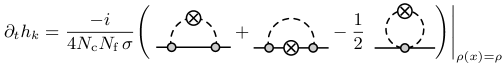
Figure 2: Diagrammatic representation of the flow of the Yukawa coupling. The grey circles depict the full vertices.

The projection (30) using the fermionic two-point function is directly related to the more customary projection where an additional derivative with respect to the pion fields is applied. One finds

$$-\frac{i}{\sigma}\text{Tr}\left(\partial_{t}\Gamma_{k}^{(\psi\bar{\psi})}\right)=\left.\text{Tr}\left(\gamma_{5}\vec{\tau}\,\partial_{\vec{\pi}}\partial_{t}\Gamma_{k}^{(\psi\bar{\psi})}\right)\right|_{\vec{\pi}=0}\,.$$

Note that a projection using an additional derivative with respect to the sigma field would contaminate the flow with additional contributions from the derivative of the Yukawa coupling.

With (30) we find for the flow of the renormalised Yukawa coupling:

$$\begin{split}&\left.\partial_{t}\right|_{\rho}\bar{h}_{k}(\bar{\rho})=\\ &\qquad\Bigl{(}\frac{1}{2}\eta_{\phi,k}+\eta_{\psi,k}\Bigr{)}\bar{h}_{k}(\bar{\rho})\\ &\qquad+4v_{3}\bar{h}_{k}^{3}(\bar{\rho})\left[L_{(1,1)}^{(4)}\left(\bar{m}_{\psi,k}^{2},\bar{m}_{\sigma,k}^{2},\eta_{\psi,k},\eta_{\phi,k};T,\mu\right)\right.\\ &\qquad\left.-(N_{\text{f}}^{2}-1)\,L_{(1,1)}^{(4)}\left(\bar{m}_{\psi,k}^{2},\bar{m}_{\pi,k}^{2},\eta_{\psi,k},\eta_{\phi,k};T,\mu\right)\right]\\ &\qquad+16v_{3}\bar{h}_{k}(\bar{\rho})\bar{h}^{\prime}_{k}(\bar{\rho})\bar{\rho}\Bigl{[}\bar{h}_{k}(\bar{\rho})+\bar{\rho}\bar{h}^{\prime}_{k}(\bar{\rho})\Bigr{]}\\ &\qquad\times L_{(1,1)}^{(4)}\left(\bar{m}_{\psi,k}^{2},\bar{m}_{\sigma,k}^{2},\eta_{\psi,k},\eta_{\phi,k};T,\mu\right)\\ &\qquad-2v_{3}k^{2}\Bigl{[}\left(3\bar{h}^{\prime}_{k}(\bar{\rho})+2\bar{\rho}\bar{h}^{\prime\prime}_{k}(\bar{\rho})\right)l_{1}^{(B,4)}(\bar{m}_{\sigma,k}^{2},\eta_{\phi,k};T)\Bigr{.}\\ &\qquad\Bigl{.}+3\bar{h}^{\prime}_{k}(\bar{\rho})\,l_{1}^{(B,4)}(\bar{m}_{\pi,k}^{2},\eta_{\phi,k};T)\Bigr{]}\,.\end{split}$$ (32)

The function $L_{(1,1)}^{(4)}$ is defined in Appendix B. We note that the terms proportional to $\bar{h}_{k}^{3}$ in eq. (32) are the triangle-diagram contributions to the flow of a field-independent Yukawa coupling, see e.g. Braun (2009). For the renormalised couplings (14) in (13) we find analogously to (22)

$$\begin{split}&\left.\partial_{\bar{\rho}}^{n}\left.\partial_{t}\right|_{\rho}\bar{h}_{k}(\bar{\rho})\right|_{\bar{\rho}=\bar{\kappa}_{k}}\\ &\qquad=(\partial_{t}-n\,\eta_{\phi,k})\bar{h}_{n,k}-\bar{h}_{n+1,k}(\partial_{t}+\eta_{\phi,k})\bar{\kappa}_{k}\,,\end{split}$$ (33)

where $\partial_{t}\bar{h}_{k}(\bar{\rho})$ is given by eq. (32). Hence the flows of $\bar{h}_{n,k}$ show the same decoupling properties within the expansion scheme already discussed below (22).

III.3 Wave function renormalisations

As discussed at the end of Section II.1, at finite temperature the wave function renormalisations perpendicular and parallel to the heat bath differ from each other, $Z_{k}^{\perp}\!\neq\!Z_{k}^{\parallel}$. For scales above the chiral symmetry breaking scale, $k>k_{\chi\text{SB}}$, we have $T/k<1$ which implies that thermal fluctuations are negligible and thus $Z_{k>k_{\chi\text{SB}}}^{\perp}\approx Z_{k>k_{\chi\text{SB}}}^{\parallel}$. In the infrared we have $k\!\ll\!T$. In this regime dimensional reduction occurs and we approach the three-dimensional limit. There the finite temperature RG flow is only driven by the lowest Matsubara modes. The lowest Matsubara mode for bosons is zero and therefore $Z_{\phi,k\ll T}^{\parallel}$ drops out. For fermions the lowest Matsubara mode is proportional to $T$ and thus the fermions with dynamically generated mass effectively decouple from the flow in the infrared. Therefore we choose the approximation $Z_{k}\!=\!Z_{k}^{\perp}\!=\!Z_{k}^{\parallel}$, which is approximately valid for large scales and hardly affects the RG flow in the infrared. Hence it should be a good approximation for calculating the chiral phase boundary.

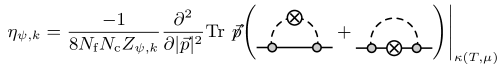
Figure 3: Diagrammatic representation of the quark anomalous dimension.

The flow of (6) consistent with the expansion scheme about $\rho=\kappa$ has to involve an evaluation of the two-point function at the expansion point. As the momentum dependence is covered in a coarse-grained form via the $k$-dependence of the $Z_{k}$’s, we also use the derivative expansion about the lowest momentum and frequency and arrive at

$$\eta_{\psi,k} = -\frac{1}{8N_{\text{f}}N_{\text{c}}Z_{\psi,k}}$$

$$\!\times\text{Re}\left[\lim_{p\rightarrow p_{\text{low}}}\frac{\partial^{2}}{\partial|\vec{p}|^{2}}\text{Tr}\left.\left(\vec{\gamma}\vec{p}\,\frac{\delta^{2}\partial_{t}\Gamma_{k}}{\delta\psi(-p)\delta\bar{\psi}(p)}\right)\right|_{\rho=\kappa}\right]\,,$$

for the anomalous dimension $\eta_{\psi,k}$ defined in (19). We note that, analogous to the computation of the Yukawa coupling, the projection onto external momentum $p_{\text{low}}$ also renders the flow on the right hand side complex valued. Similarly to the Yukawa coupling, the anomalous dimension is a function of the complex variable $(p_{0}-i\mu)$, and projecting onto the real part, see (III.3), keeps all properties and symmetries intact. This leads to

$$\eta_{\psi,k}= \frac{2v_{3}}{3}\left(4-\eta_{\phi,k}\right)$$

$$\times\Bigl{[}(N_{\text{f}}^{2}-1)\,\bar{h}_{k}(\bar{\kappa}_{k})^{2}\mathcal{FB}_{(1,2)}\left(\bar{m}_{\psi,k}^{2},\bar{m}_{\pi,k}^{2};T,\mu\right)\Bigr{.}$$

$$+\Bigl{.}\Bigl{(}\bar{h}_{k}(\bar{\kappa}_{k})+2\bar{\kappa}_{k}\,\bar{h}_{k}^{\prime}(\bar{\kappa}_{k})\Bigr{)}^{\!2}\Bigr{.}$$ (35)

$$\times\,\Bigl{.}\mathcal{FB}_{(1,2)}\left(\bar{m}_{\psi,k}^{2},\bar{m}_{\sigma,k}^{2};T,\mu\right)\Bigr{]}.$$

The function $\mathcal{FB}_{(1,2)}^{(4)}$ is defined in Appendix B. In the case of one quark flavour and for $\bar{h}_{k}^{\prime}=0$ this equation agrees with that found in Braun (2010). The diagrammatic representation of equation (III.3) is shown in Fig. 3.

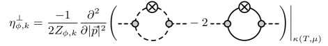
Figure 4: Diagrammatic representation of the meson anomalous dimension.

The anomalous dimension of the mesons can be either extracted by taking derivatives w.r.t. $\sigma$ or $\pi$. Here, a similar argument as for the flow of the Yukawa coupling (Section III.2) applies and we choose the following projection:

$$\eta_{\phi,k}=-\frac{1}{2Z_{\phi,k}}\lim_{p\rightarrow p_{\text{low}}}\frac{\partial^{2}}{\partial|\vec{p}|^{2}}\text{Tr}\left.\left(\frac{\delta^{2}\partial_{t}\Gamma_{k}}{\delta\pi_{i}(-p)\delta\pi_{i}(p)}\right)\right|_{\rho=\kappa(T,\mu)},$$ (36)

where the choice of $i=1,2,3$ does not matter since the pions always have $O(3)$ symmetry in this representation. This leads to

$$\begin{split}\eta_{\phi,k}=&\frac{8v_{3}}{3}\Bigl{\{}2k^{-2}\bar{\kappa}_{k}\,(\bar{V}_{k}^{\prime\prime}(\bar{\kappa}_{k}))^{2}\,\mathcal{BB}_{(2,2)}\left(\bar{m}_{\pi,k}^{2},\bar{m}_{\sigma,k}^{2};T,\mu\right)\Bigr{.}\\ &+\Bigl{.}N_{\text{f}}N_{\text{c}}\bar{h}_{k}(\bar{\kappa}_{k})^{2}\left[\left(2\eta_{\psi,k}-3\right)\mathcal{F}_{(2)}(\bar{m}_{\psi,k}^{2};T,\mu)\right.\Bigr{.}\\ &-\Bigl{.}\left.4\left(\eta_{\psi,k}-2\right)\mathcal{F}_{(3)}(\bar{m}_{\psi,k}^{2};T,\mu)\right]\Bigr{\}}.\end{split}$$ (37)

The functions $\mathcal{BB}_{(2,2)}^{(4)}$ and $\mathcal{F}_{(n)}^{(4)}$ are defined in Appendix B. This equation also agrees with Braun (2010) for one quark flavour. We note that the results shown here are obtained using the optimised regulator shape functions (56). The diagrammatic representation of (37) is shown in Fig. 4.

We want to emphasize again that the wave function renormalisations are defined as the zeroth order of an expansion about $\bar{\kappa}_{k}$. From (III.3) and (37) it is clear that we can define the wave function renormalisations at any expansion point. Defining them at $\bar{\kappa}_{k}$ is the consistent way to define the renormalized couplings related to the Yukawa coupling and the effective potential since these couplings are defined at $\bar{\kappa}_{k}$ as well. For the definition of the physical parameters, e.g. the masses, however, we make use of the option to freely choose the expansion point and evaluate the wave function renormalisations at the minimum $\bar{\rho}_{0,k}$, see appendix A.

The wave function renormalisations as a function of temperature are shown in Fig. 5. At about the critical temperature $Z_{\psi,\text{IR}}$ exhibits a peak and $Z_{\phi,\text{IR}}$ shows a tiny kink. This kink gets more pronounced and turns into a dip for smaller pion masses and ends up as a non-analyticity in the chiral limit Berges et al. (1999). An interesting observation is that the meson wave function renormalisation falls below its initial value in the UV for temperatures above $200$ MeV. This feature is independent of the choice of the UV value and shows that mesonic degrees of freedom become less important for larger temperatures in the crossover region and vanish in the symmetric phase. The inclusion of a dynamical meson wave function renormalisation therefore leads to a consistent picture of the QCD matter sector in the sense that mesons are only present in the phase with broken chiral symmetry, while they vanish (or rather turn into auxiliary fields) in the symmetric phase where quarks and gluons are the relevant degrees of freedom.

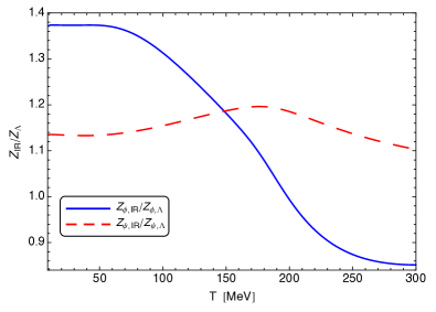
Figure 5: Temperature dependence of the wave function renormalisations in the IR, normalised to their values in the UV.

III.4 Convexity for $\rho<\rho_{0}$ & behaviour for large fields

The flows are initiated at a UV cut-off scale $k=\Lambda$. There, the initial effective action $\Gamma_{\Lambda}$ resembles the classical Yukawa theory with a $\phi^{4}$-potential and a constant Yukawa coupling. This entails that all flows decay in the limit where $\rho/k^{2}\to\infty$, and we conclude

$$\begin{split}\partial_{t}\bar{h}_{k}(\rho/k^{2}\rightarrow\infty)=0\,\quad{\rm and}\quad\partial_{t}\bar{V}_{k}(\rho/k^{2}\rightarrow\infty)=0\,.\end{split}$$ (38)

Hence, neither the Yukawa coupling nor the effective potential are changed during the flow for large enough fields.

For the convexity discussion it is sufficient to restrict ourselves to the chiral limit. As already mentioned before the explicit symmetry breaking does not influence the dynamics of the fluctuations which are solely responsible for the convexity properties. It is well-known that the effective potential $V_{k=0}$ is convex by construction. It has been shown that the flow equation is indeed convexity-restoring in the limit $k\to 0$ and keeps this property in the local potential approximation, see Litim et al. (2006). This implies in particular, that the the curvature of the effective potential vanishes for field values smaller than their vacuum expectation value, $\partial_{\phi}^{2}V_{k=0}(\rho\!<\!\rho_{0})=0$. For non-vanishing cut-off scale, $k>0$, only the combination $V_{k}(\rho)+\rho\,R_{k}^{\phi}(0)$ is convex. This property follows directly from its definition as the Legendre transformation of the logarithm of the generating functional $\ln Z_{k}[J]$, evaluated on constant fields and divided by the space-time volume, for a detailed discussion see e.g. Pawlowski (2007). This entails in particular

$$V^{\prime}_{k}(\rho)+R_{k}^{\phi}(0)\geq 0\,,\quad V^{\prime}_{k}(\rho)+2\rho V^{\prime\prime}(\rho)+R_{k}^{\phi}(0)\geq 0\,,$$ (39)

for the inverse propagator pion and $\sigma$-meson propagator respectively at vanishing momentum. In the chirally broken phase with $\rho<\rho_{0,k}$ we have

$$V^{\prime}_{k}(\rho<\rho_{0,k})<0\quad{\rm and}\quad V^{\prime}_{k=0}(\rho<\rho_{0})=0\,,$$ (40)

with $\rho_{0}$ is the vaccuum expextation value $\rho_{0,k}$ at vanishing cut-off scale, $k=0$. Note that (40) also implies $V^{\prime\prime}_{k=0}(\rho<\rho_{0})=0$. Of course, (40) entails that the potential $V_{0}$ is flat (vanishing curvature) for fields $\rho$ smaller than the vaccuum expectation value. Note that for negative $V^{\prime}$ the inverse pion propagator in (39) vanishes for $V^{\prime}=R_{k}^{\phi}(0)$, and the flow potentially diverges for $R_{k}^{\phi}(0)\to 0$. However, this divergence is not reached as the increasing flow increases $V^{\prime}$, see Litim et al. (2006) for a discussion of a scalar theory. In Appendix C this discussion is extended to the present Yukawa theory.

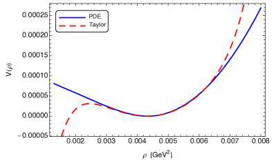
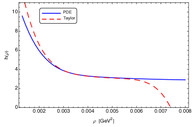
Figure 6: Effective potential (left) and Yukawa coupling (right) at cut-off scale $k\!=\!0.1\,\text{MeV}$ within the Taylor expansion and the full solution of the coupled partial differential flow equations for $\eta_{\psi,k},\eta_{\phi,k}$, $V_{k}(\rho)$ and $h_{k}(\rho)$ at $T\!=\!10\,\text{MeV}$ and $\mu\!=\!0$. For the Taylor expansion we used $N_{V}=7$ and $N_{h}=5$. Note that the results include the explicit $O(4)$ symmetry breaking via $-c\sigma$.

The relation between the negative curvature $V^{\prime}$ and the convexity-restoration in the flow also implies that only the mesonic fluctuations drive the flows for $\rho<\rho_{0}$ and $k\to 0$, and the two sectors effectively decouple. This facilitates the access to the infrared flow of the fermion propagator in this region studied in detail in Appendix C, which can indeed be derived analytically. We arrive in particular at

$$\bar{m}_{\psi}^{2}(\rho\leq\rho_{0})=\sqrt{2\rho_{0}}\bar{h}(\rho_{0},0)\frac{\rho_{0}}{\rho}\,,$$ (41)

see (76) in Appendix C. In this appendix a momentum-dependent Yukawa coupling $h(\rho,p)$ has been introduced. In (41) it is evaluated at vanishing momentum, $h(\rho,0)$. This leads to the inequality

$$\bar{m}_{\psi}^{2}(\rho)\geq\bar{m}^{2}_{\psi,\rm gap}\,,\quad{\rm with}\quad\bar{m}^{2}_{\psi,\rm gap}=\sqrt{2\rho_{0}}\bar{h}(\rho_{0},0)\,,$$ (42)

for $k=0$, see (77) in Appendix C, where we have also used the fact that for $\rho>\rho_{0}$ the mass function grows. As a consequence of (42) the fermion propagation is gapped with at least the constitutent quark mass $\bar{m}^{2}_{\psi,\rm gap}$ for all fields. In other words, in the chirally broken phase no mesonic background can turn the fermionic dispersion into a massless one. Note however, that $\rho<\rho_{0}$ is no physical choice in the first place.

We finally remark that the same line of argument can also be applied to full QCD and also holds there. There however, the fermionic mass tends towards the current quark masses for large meson fields $\rho$ and the minimum in (42) has to be restricted to $\rho\lesssim\rho_{0}$. In the present model a linearly rising mass was built-in and strictly speaking one should not evaluate the model for $\rho/\Lambda^{2}\gg 1$ in the first place. The full discussion of QCD is postponed to future work.

IV Set-up and Results

IV.1 Initial conditions in the UV

It is left to specify the initial conditions for the relevant parameters $\lambda_{1,k},\lambda_{2,k},h_{0,k}$ and $c_{k}$ at the UV-scale $\Lambda$ for the system of coupled flow equations (16), (22), (24), (33), (III.3) and (37). As we have mentioned in section II, the effective UV-cutoff scale $\Lambda$ has a direct physical meaning in our setting. It is the scale where the dominant part of the gluonic degrees of freedom has been integrated out and hadronic degrees of freedom, especially the light mesons, form. There is a certain freedom in the choice of this scale as long as it is well above $\Lambda_{\text{QCD}}$ and not too large so that fluctuations in the gauge sector dominate the dynamics. This requirements bring forth $\Lambda\in[0.6,1]\,\text{GeV}$ as an approximate window for the choice of the UV-cutoff.

As discussed in Section III we have chosen $\Lambda=700\,\text{MeV}$. The relevant parameters of our model are fixed such that a specific set of vacuum low-energy observables is reproduced in the in the IR. These observables are the pion decay constant $f_{\pi}$, the renormalized sigma and pion masses $\bar{m}_{\sigma},\,\bar{m}_{\pi}$ and the constituent quark mass $\bar{m}_{q}$ of the degenerate up and down quarks. The explicit symmetry breaking is related to the pion decay constant and the pion mass via $\bar{c}_{k}=\bar{m}_{\pi}^{2}f_{\pi}$ and the relations of our parameters to the quark and mesons masses are shown in eq. (21) and (20). At a large scale $\Lambda$ the model is quasi-classical and hence we choose

$$\begin{split}\bar{V}_{\Lambda}(\bar{\rho})&=\frac{\bar{\lambda}}{2}(\bar{\rho}-\bar{\nu})^{2}\\ \bar{h}_{\Lambda}(\bar{\rho})&=\bar{h}=\text{const.}\end{split}$$ (43)

The underlying assumption is that at $\Lambda$ the dynamics are controlled by the leading order processes, i.e. the four-meson and the quark-antiquark-meson scattering. The higher order couplings are generated at lower scales $k<\Lambda$. We indeed found that the higher order operators, i.e. $\bar{\lambda}_{n,k}$ with $n\geq 3$ and $\bar{h}_{m,k}$ with $m\geq 1$ are generated at $k\lesssim 400\,\text{MeV}$, which is well below our choice for the UV-cutoff. Since the higher order operators are not present at our initial scale, the scale where they are generated is a prediction of our model.

In order to reproduce the vacuum IR-observables listed above we used the following initial values: $\bar{\lambda}=71.6,\,\bar{\nu}=0,\,\bar{h}=3.6,\,\bar{c}_{\Lambda}=2.1\cdot 10^{-3}\,\text{GeV}^{3}$. These initial values result in the following values for the vacuum IR-observables,

$$\begin{split}f_{\pi}&=93.0\,\text{MeV}\\ \bar{m}_{\pi}&=138.7\,\text{MeV}\\ \bar{m}_{\sigma}&=538.2\,\text{MeV}\\ \bar{m}_{q}&=298.3\,\text{MeV},\end{split}$$ (44)

which are in good agreement with their values provided by the Particle Data Group Beringer et al. (2012). The initial values of the parameters for the present computations are chosen such that they reproduce the vacuum physics displayed in (44) for $T,\mu=0$ and vanishing cut-off for the fully field-dependent effective potential $\bar{V}_{k}(\bar{\rho})$ and Yukawa coupling $\bar{h}_{k}(\bar{\rho})$, including running wave function renormalisations $Z_{\phi,k}$ and $Z_{\psi,k}$. With the convergence pattern discussed in the next section it is sufficient to use $N_{V}=7$ and $N_{h}=5$ in the expansions (7) and (12), and fix the initial parameters for these values.

The bare expansion point $\kappa(T,\mu)$ is chosen to be scale-independent. We take it close to the IR-minimum of the effective potential for every temperature and chemical potential:

$$\bar{\kappa}_{\text{IR}}(T,\mu)=(1+\epsilon)\,\bar{\rho}_{0,\text{IR}}(T,\mu),$$ (45)

where $\epsilon>0$ gives a small offset that guarantees that $\bar{\kappa}_{k}(T,\mu)$ is always slightly larger than the minimum of the effective potential $\bar{\rho}_{0,k}$ and does not lie in the flat region of the convex effective potential $V_{k=0}$. The details are deferred to Appendix A. It can be read-off from Fig. 11 that a quantitative agreement of the physics results is obtained for expansion points in the range

$$0\leq\epsilon\lesssim 1\,.$$ (46)

This self-consistency check within the present expansion scheme is impressively sustained by the comparison with the full solution of the system of partial different equations for $V_{k}(\rho)$, $h_{k}(\rho)$, $\eta_{\phi,k}(\bar{\kappa}_{k})$ and $\eta_{\psi,k}(\bar{\kappa}_{k})$, see Fig. 6. The region where the results from the Taylor expansion and the full solution of the partial differential equation agree give an estimate for the radius of convergence of the Taylor expansion. This is in agreement with the study of the robustness of the expansion in Appendix A and in particular with Fig. 11.

IV.2 Effect of higher order mesonic interactions on the chiral order parameter

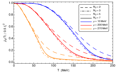
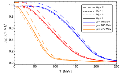
Figure 7: The normalised chiral order parameter as a function of temperature for different orders in the expansion of the effective potential (left) and the Yukawa coupling (right).

The effect of higher order mesonic operators is studied within a Taylor expansion of the effective potential and the field dependent Yukawa coupling, see section II.2. This is done by comparing the results of the chiral order parameter for different orders $N_{V}$ and $N_{h}$ in the expansions (7) and (12) of the effective potential and the field dependent Yukawa coupling. In Fig. 7 we show the effect of increasing $N_{V}$ and $N_{h}$ on the chiral order parameter $\bar{\rho}_{0,\text{IR}}$ as function of temperature for three different chemical potentials.

First of all, we clearly see spontaneous chiral symmetry breaking. Owing to the explicit symmetry breaking, the chiral condensate is very small, but nonzero at large temperatures. By lowering the temperature, the fluctuations of the light current quarks drive the system continuously towards the broken phase. As the value of the chiral condensate increases, the quarks receive more and more constituent mass while the pions get lighter until quarks and mesons decouple at low temperatures where the flow stops and the system ends up in the stable phase with broken chiral symmetry. The quark and meson masses as a function of temperature at $\mu=0$ are shown in Fig. 8. Note that the decreasing slope of the meson masses at temperatures $T\gtrsim 250\,\text{MeV}$ is a result of thermal fluctuations which become of the order of the UV-cutoff $\Lambda$ in this region. This is discussed in detail in Herbst et al. (2013a).

With increasing quark chemical potential, quark fluctuations are enhanced and the crossover gets steeper while the transition moves towards smaller temperatures as a result of the higher quark density.

Note that since the transition is a cross-over the actual value of the critical temperature $T_{c}$ depends on the the definition of the crossover. In this case it is only sensible to speak about a transition region. Therefore the full temperature and chemical potential dependence of the observables used to define the critical temperature plays a more important role than the specific critical values.

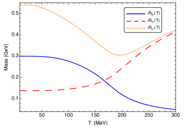
Figure 8: Quark, pion and sigma mass as a function of Temperature for vanishing chemical potential.

The left panel in Fig. 7 shows the chiral order parameter in the IR normalised to the pion decay constant for different orders $N_{V}=2,\,3,\,5,\,7$ of the expansion of the effective potential for $\mu=10\,\text{MeV},\,200\,\text{MeV},\,270\,\text{MeV}$ and a fixed order $N_{h}=2$ in the expansion of the Yukawa coupling. Note that we chose $N_{h}$ such that $N_{h}\leq N_{V}$ for numerical stability. While $\rho_{0}(T)$ is hardly affected by different $N_{V}$ in the broken phase at small temperatures, we see a large difference between the $\phi^{4}$ and the $\phi^{14}$ expansion in the lower region of the crossover transition. This effect gets more pronounced for larger chemical potentials. There is a very good agreement between the order parameter for $N_{V}=5$ and $N_{V}=7$ which implies that the expansion of the effective potential at order $N_{V}=5$ has converged to a precision of the critical temperature below $1$ MeV. We explicitly checked that larger orders in the expansion do not spoil this observation.

The effect of the expansion of the field dependent Yukawa coupling on the chiral condensate is shown in the right panel of Fig. 7. The difference between the usual running Yukawa coupling $N_{h}=0$ and the expansion of order $N_{h}=5$ is at about $8\%$ which results in a difference of $8\!-\!10$ MeV in the critical temperature. The expansion of order $N_{h}=4$ seems to be converged to a precision of the critical temperature below $1$ MeV. We observed that larger chemical potential slows down the convergence of the Yukawa coupling. This behaviour is expected since a larger chemical potential effectively increases quark fluctuations and thus the systems is more sensitive to the details of the quark-meson interactions.

We see that the particular meson-meson and quark-meson interactions we have chosen here have a large quantitative effect on the chiral order parameter. Moreover we nicely see that these higher order operators a become increasingly irrelevant with increasing order of the meson fields and that our expansion converges rapidly, especially for not too large chemical potential. This implies in particular that we have the full effective potential as well as the full field-dependent Yukawa coupling in this region. To demonstrate this, we solved the coupled partial differential flow equations of $V_{k}(\rho)$, $h_{k}(\rho)$, $\eta_{\phi,k}(\bar{\kappa}_{k})$ and $\eta_{\psi,k}(\bar{\kappa}_{k})$ and compared the result to the one obtained with the expansion employed in this work, see Fig. 6.

Note that, as expected, the couplings with negative mass dimension run into a Gaussian fixed point in the IR but certainly play a role at intermediate scales. Furthermore, it is obvious that a low-order expansion is not sufficient in order to obtain a high degree of quantitative precision.

IV.3 Phase diagram

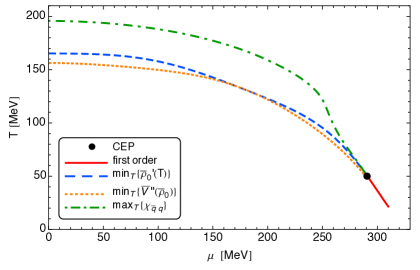
Figure 9: The phase diagram of the chiral transition including the different definitions of the crossover transition line we used. We only show the first order transition up to $\mu=310\,\text{MeV}$ since our expansion is not fully converged for larger $\mu$, see Appendix A.

IV.3.1 Phase structure

For the computation of the phase diagram, we expand the effective potential up to order $N_{V}=7$ and the Yukawa coupling up to $N_{h}=5$. According to the previous section, these orders guarantee that both expansions converged to a precision below 1 MeV, at least in the crossover region. The resulting phase diagram in the $(T,\mu)$-plane is shown in Fig. 9. The crossover transition temperature is not uniquely defined and therefore depends on the observable used to define it. Basically any observable that exhibits a non-differentiable behaviour at the critical temperature in the chiral limit, where the transition is of second order, can be used to define the crossover transition temperature. Here we use the following three definitions:

• The inflection point of the chiral order parameter as a function of temperature,

  $$\min_{T}\left\{\frac{\partial\bar{\rho}_{0,\text{IR}}}{\partial T}\right\}.$$ (47)

• The minimum of the quartic meson coupling at the physical point,

  $$\min_{T}\left\{\left.\frac{\partial^{2}\bar{V}_{\text{IR}}(\bar{\rho})}{\partial\bar{\rho}^{2}}\right|_{\bar{\rho}=\bar{\rho}_{0,k}}\right\}.$$ (48)

• The maximum of the chiral susceptibility (26),

  $$\max_{T}\left\{\chi_{\bar{q}q}\right\}.$$ (49)

The definition (i) is commonly used in RG-studies of the phase diagram, while susceptibilities as in (iii) are typically used in lattice gauge theory. The exact location and in particular the curvature of the phase boundary obviously depend on the definition of the crossover. Note, however, that all the definitions above exactly agree in the chiral limit.

We observe a large difference of about 40 MeV in the critical temperature at small and intermediate chemical potential between definitions (i) and (iii), while (i) and (ii) give similar phase boundaries. These differences are related to the fact that we have a very broad crossover in this region and the notion of a phase transition line is certainly not well defined there. At large chemical potential close to the critical point the crossover lines merge and give a uniquely defined phase boundary. This behaviour is expected since the crossover gets steeper towards the critical point and the first-order transition is uniquely defined. We find the critical endpoint at $(T_{\text{CEP}},\mu_{\text{CEP}})=(50,291)\,\text{MeV}$. The critical endpoint here is at substantially smaller temperatures as in mean-field studies, see e.g. Schaefer et al. (2007). This nicely demonstrates the effect of fluctuations on the phase boundary. The critical temperatures at vanishing chemical potential for the different definitions of the crossover transition are show in table 1.

boundary def.	$T_{c}\,[\text{MeV}]$
(i)	166
(ii)	156
(iii)	196

Table 1: Critical temperatures at vanishing quark chemical potential for the different definitions of the crossover phase boundary we used in this work (see text).

A further definition of a cross-over temperature in the literature is given by the temperature where the value of the normalised order parameter is half of that at vanishing temperature, $\rho_{0,\text{IR}}(T,\mu)/\rho_{0,\text{IR}}(0,0)=0.5$. Here we only note that the critical temperature at $\mu\!=\!0$ is $T_{c}\!=\!152$ MeV and the transition line is systematically below the lines shown in Fig. 9. This behavior is in contrast to studies of the quark-meson model in the local potential approximation, where this phase boundary is always slightly above the boundary defined by (i), see e.g. Herbst et al. (2013b).

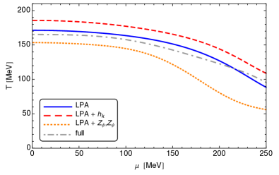
Figure 10: Comparison of the phase boundary for different truncations of the quark-meson model. The solid blue line corresponds to the local potential approximation (LPA), i.e. a truncation with only a running effective potential. For the dashed red curve also a running (field-independent) Yukawa coupling was taken into account and for the dotted orange curve we have running quark and meson wave function renormalisations and the effective potential, but a constant Yukawa coupling. The dot-dashed gray curve shows the full result of our model. Here, we defined the crossover transition via definition (i), see text.

The inclusion of running wave function renormalisations enhances the symmetry-preserving mesonic fluctuations and therefore decrease the critical temperature. In turn, the transition temperature is increased if a the running Yukawa coupling is taken into account. This is shown in figure 10. Note that we used the initial conditions specified in IV.1. This ensures that for every truncation used in figure 10 we start with the same effective action at the initial scale $\Lambda$. This approach is motivated by the fact that in principle the initial conditions at $\Lambda$ are uniquely defined by the solution of full QCD at scales $k\geq\Lambda$.

IV.3.2 Curvature

In order to determine the curvature of the chiral phase boundary, we compute $T_{c}(\mu)/T_{c}(0)$ in a range $0\leq\mu/(\pi T_{c}(0))\lesssim 0.1$ and extract the curvature of the phase boundary at vanishing chemical potential from these results. At small chemical potential the phase boundary can be expanded in powers of $\mu^{2}$ as follows:

$$\frac{T_{c}(\mu)}{T_{c}(0)}=1-\kappa_{\mu}\left(\frac{\mu}{\pi T_{c}(0)}\right)^{2}+\mathcal{O}\biggl{(}\!\left(\frac{\mu}{\pi T_{c}(0)}\right)^{4}\biggr{)}.$$ (50)

The curvature $\kappa_{\mu}$ depends on the number of colours $N_{\text{c}}$, the number of quark flavours $N_{\text{f}}$ and the current quark mass or the pion mass respectively, see e.g. Braun (2009). But since all those parameters are fixed in the present work, we do not study the effect of variations of them. For a crossover transition the curvature depends on the definition of the phase boundary. For our result in comparison with lattice results and other RG calculations see table 2. We extracted the curvature from a fit of the phase boundary according to (50) for $\mu\in[0,20]$ MeV. The errors result from fits with polynomials of the order $\mu^{2},\,\mu^{4},\,\mu^{6}$.

Compared to the curvature found in Braun et al. (2012), the inclusion of higher order mesonic scattering processes and dressed quark and meson propagators does not change the curvature much. This is related to the observation that running wave function renormalisations and the running Yukawa coupling have opposing effects on the phase boundary, see also Fig. 10.

method	boundary def.	mass	$\kappa_{\mu}$
Lattice: $i\mu$ de Forcrand and Philipsen (2002)	plaquette susc.	$am=0.025$	$0.500(54)$
FRG: LPA Schaefer and Wambach (2005)	$\min_{T}\{\rho_{0}^{\prime}(T)\}$	chiral limit	$1.135$
FRG: LPA Braun et al. (2012)	$\min_{T}\{\rho_{0}^{\prime}(T)\}$	$m_{\pi}=138$ MeV	$1.375(63)$
this work: LPA	$\max_{T}\{\chi_{\bar{q}q}\}$	$m_{\pi}=138$ MeV	$1.397(1)$
this work: full model (1)	$\min_{T}\{\rho_{0}^{\prime}(T)\}$	$m_{\pi}=138$ MeV	$1.397(2)$
	$\max_{T}\{\chi_{\bar{q}q}\}$		$1.418(13)$
	$\min_{T}\{\bar{V}^{\prime\prime}(\bar{\rho}_{0})\}$		$0.794(1)$

Table 2: This table shows the curvature of the chiral phase boundary for $N_{f}=2$ quark flavours obtained from various methods. $am$ is the lattice spacing times the degenerate current quark mass. The last three rows correspond to the different boundary definitions we employed in this work.

Owing to our findings in the previous section we certainly need to use the same definition of the phase boundary as in de Forcrand and Philipsen (2002) in order to do a sensible comparison with the lattice results. But since they used the plaquette susceptibility for the definition of the critical temperature, a direct comparison is difficult since gluonic quantities are not directly accessible in our model. We therefore displayed the results for the curvature for different boundary definitions. We see that while the curvatures extracted from the chiral order parameter and the chiral susceptibility are very similar but much larger than the lattice results, the curvature from the quartic meson coupling is close the lattice result. We see that these results very much depend on the specific definition of the crossover temperature, in line with our findings in the previous section.

We note that it was observed for QM-model studies that the curvature increases with increasing pion mass Braun et al. (2012), which explains the difference between the curvature found in Schaefer and Wambach (2005) and in Braun et al. (2012), where very similar truncations were used but one in the chiral limit and the other at realistic pion masses. This is in contrast to the general expectation that the system gets less sensitive to the chemical potential for larger current quark mass.

V Conclusions and Outlook

In this work, we have investigated the impact of higher order mesonic scattering processes on the matter sector of two-flavour QCD at finite temperature and quark chemical potential. Quantum, temperature and density fluctuations have been taken into account within a renormalisation group analysis of a quark-meson model. In particular, we have introduced for the first time a meson-field dependent Yukawa coupling. The effect of higher order meson-meson and quark-meson operators has been systematically studied by expanding both the Yukawa coupling and the effective potential in orders of the meson fields. These higher order operators play a quantitatively important role for the chiral phase transition. Furthermore, we observed that these operators become increasingly irrelevant with increasing order of the meson fields, see Fig. 7. This indicates a rapid convergence of the expansion scheme we used and allows us to have certain control over the quantitative precision of our results.

We have computed the phase diagram of the chiral transition at finite temperature and quark chemical potential, see Fig. 9. Owing to the explicit $O(4)$-symmetry breaking which is directly related to finite current quark masses we see a broad crossover phase transition for $\mu<291$ MeV. Crossover temperatures cannot be defined uniquely. In the present work we have compared standard definitions for the phase boundary and the corresponding temperatures show the expected large deviations. In particular this implies large differences in both the critical temperature at vanishing chemical potential and the curvature. In the chiral limit, all definitions provide the same results.

At large chemical potential close to the critical point the phase boundary is again uniquely defined since the crossover gets steeper in this region. Even though we employed a local expansion of the effective potential in this work, our particular expansion scheme allowed us to resolve some global features of the effective potential. This way we could capture the first order phase transition for not too small temperatures and we found a critical endpoint at $(T_{\text{CEP}},\mu_{\text{CEP}})=(50,291)\,\text{MeV}$.

Note, however, that at large chemical potential and small temperatures quark-meson models in the present approximation are not expected to give an accurate description of the QCD phase structure since diquark and baryonic fluctuations should play an important role in this region. Within the present approximation they are only taken into account implicitly, the improvement of the present work in this direction will be discussed elsewhere.

Acknowledgments - We thank Jens Braun, Lisa Marie Haas, Tina K. Herbst, Naseemuddin Khan, Mario Mitter, Daisuke Sato, Bernd-Jochen Schaefer, Nils Strodthoff, and Masatoshi Yamada for discussions and collaboration on related subjects. JMP thanks the Yukawa Institute for Theoretical Physics, Kyoto University, where this work was completed during the YITP-T-13-05 on ’New Frontiers in QCD’. This work is supported by Helmholtz Alliance HA216/EMMI and by ERC-AdG-290623.

Appendix A Expansion scheme

In this Appendix technical details and convergence properties of the present expansion scheme are discussed. Most expansion schemes in the literature are either based on a discretisation of the effective potential in field-space or a Taylor expansion about the scale dependent minimum of the effective potential. The latter approach is very efficient for low-order truncations with many different interaction channels and has been proven to be very successful at the description of critical phenomena (see e.g. Litim (2002)). The former gives a very detailed global picture of the effective potential and is therefore well suited to study first order phase transitions. Our expansion scheme may be seen as a compromise between both approaches without being numerically extensive. It is easily possible to include various directions in parameter space into the truncation while maintaining global information about the effective potential to a good accuracy.

A.1 Background dependence

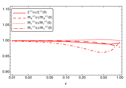
Figure 11: Dependence of the IR-observables on the offset parameter $\epsilon$. Our results for the observables are very robust with respect to variations of the expansion point if we take the corrections (52) into account, implying a high degree of convergence of our expansion.

Instead of doing an expansion about the scale-dependent minimum of the effective potential $\rho_{0,k}$, we expand the non-renormalised theory about a scale-independent field configuration $\kappa$, see (4), (9) and (13). Technically, the advantage is that there is no unnecessary feedback from the expansion point into the flow of higher order operators. In an expansion about the minimum of the effective potential the flow of the minimum feeds back into the flow of every higher order operator, see the discussion below (22). This feedback slows down numerical computations and potentially leads to numerical instabilities. But even though the minimum certainly is a distinct point in the effective potential, it is by no means distinct in the flow of the effective potential. The same holds true for the flow of the effective action in general. In principle it is therefore irrelevant whether one solves the flow equations with an expansion about $\bar{\rho}_{0,k}$ or any other point in field space. $\bar{\rho}_{0,k}$ can always be extracted from $\bar{V}_{k}(\bar{\rho})$ from eq. (25) and enters the physical parameters such as the physical masses, $\bar{m}_{k}^{(\text{phys})}=\bar{m}_{k}(\bar{\rho}_{0,k})$.

There are two main restrictions we have for the choice of the expansion point $\kappa$. The first and most important is that $\kappa$ always has to be larger or equal to $\rho_{0,k}$ for small $k$. The reason is that for $k\rightarrow 0$ the effective potential becomes a convex function of $\rho$ which is flat for $\rho<\rho_{0,k=0}$ and we can not expect to capture the relevant features of the theory with an expansion in a potentially flat region of the potential, especially since all the physical information is stored in the effective potential and its derivatives at the minimum. However, we can extract all the information we need at much larger scales since the RG-flows of the physical parameters stop at $k\approx m_{\pi}$. The remaining flow for $k<m_{\pi}$ flattens the potential but leaves the physical parameters unchanged.

Observables are extracted at the minimum of the potential at $\bar{\rho}_{0,\text{IR}}(T,\mu)$. The present approximation has field-independent wave function renormalisations. This introduces an error which increases with the distance of the expansion point to the minimum. Consequently this leads to a finite radius of convergence in $\rho$ about the minimum, leave aside general convergence issues of the present Taylor expansion. Hence the expansion point should not be too far away from the physically relevant region. This is assured by choosing the expansion point close to the temperature and chemical potential dependent IR-minimum:

$$\bar{\kappa}_{\text{IR}}(T,\mu)=(1+\epsilon)\,\bar{\rho}_{0,\text{IR}}(T,\mu),$$ (51)

where $\epsilon$ is a small offset parameter.

The requirement of small $\epsilon$ is at least reduced qualitatively if we would also take field-dependent wave function renormalisations into account. In this work we only have considered wave function renormalisation evaluated at the expansion point, see eq. (6). Even though this is consistent with our expansion and the proper way to define RG-invariant couplings which are also defined at the expansion point, we expect some residual effects of the constant wave function renormalisations on the physical quantities that are defined at the minimum of the effective potential. In order to partially compensate for this mismatch, we redefine the renormalised IR-observables as follows:

$$\begin{split}\bar{f}_{\pi}^{(r)}&=\sqrt{Z_{\phi,\text{IR}}(\bar{\rho}_{0,\text{IR}})/Z_{\phi,\text{IR}}(\bar{\kappa}_{\text{IR}})}\,\bar{f}_{\pi},\\ \bar{m}_{\phi}^{(r)}&=\sqrt{Z_{\phi,\text{IR}}(\bar{\kappa}_{\text{IR}})/Z_{\phi,\text{IR}}(\bar{\rho}_{0,\text{IR}})}\,\bar{m}_{\phi},\\ \bar{m}_{\psi}^{(r)}&=\left(Z_{\psi,\text{IR}}(\bar{\kappa}_{\text{IR}})/Z_{\psi,\text{IR}}(\bar{\rho}_{0,\text{IR}})\right)\,\bar{m}_{\phi}.\end{split}$$ (52)

$Z_{\phi/\psi,\text{IR}}(\bar{\rho}_{0,\text{IR}})$ corresponds to the wave function renormalisations at the IR minimum of the effective potential. It is obtained from integrating the anomalous dimensions (III.3) and (37) at the physical point on the solution of the system at $\bar{\kappa}_{k}$. This ensures that the physical quantities are renormalised at the physical point in the IR and furthermore allows us to examine the robustness of our expansion even though we work with field-independent wave function renormalisations. For the sensitivity of our results on $\epsilon$ with this correction, see Fig. 11. We see that the present expansion is surprisingly robust, even though we dropped the field-dependence of the wave function renormalisations. This observation is also reflected in Fig. 6. Furthermore, given the fact that we only made a simple adjustment to the wave function renormalisations in order to define the physical observables, the robustness of our expansion already implies only a mild dependence of the wave function renormalisations on the meson fields. In the expansion (4) the zeroth order term certainly depends on the expansion point but already the first order seems to give only a small correction, otherwise we would see a much stronger dependence on the expansion point in Fig. 11.

A.2 Consistency checks

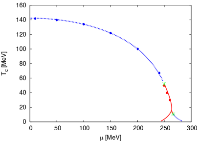
Figure 12: Phase diagram of the quark-meson model in the chiral limit from Schaefer and Wambach (2005). The blue dots and red squares show the second and first order transition points we found using the identical model and initial conditions.

Finally we present some checks concerning the validity of our expansion. Very important in the context of this work is the convergence of our expansion. This has already been demonstrated for our model in section IV.2, see Fig. 7. The convergence of other observables may be faster or slower, but the chiral condensate as a function of temperature and chemical potential is certainly the crucial observable if one is interested in the chiral phase transition.

We have determined the curvature for the quark-meson model as it is used in Braun et al. (2012) for infinite volume and found

$$\kappa_{\mu}=1.381(76),$$ (53)

which agrees with the result found in the reference.

Furthermore, we computed some points of the phase diagram of the quark-meson model in the chiral limit with the truncation used in Schaefer and Wambach (2005):

$$\begin{split}\Gamma_{k}=&\int_{0}^{\frac{1}{T}}\!dx_{0}\int\!d^{3}x\Bigl{\{}\bar{\psi}(\gamma_{\mu}\partial_{\mu}+\gamma_{0}\mu)\psi\Bigr{.}\\ &+\Bigl{.}(\partial_{\mu}\phi)^{2}+V_{k}(\rho)+h\bar{\psi}(\gamma_{5}\vec{\tau}\vec{\pi}+i\sigma\phi)\psi\Bigr{\}},\end{split}$$ (54)

where only the effective potential is running (LPA). The result is shown in Fig. 12. At vanishing temperature and density the convergence of the Taylor expansion in LPA has been checked in Papp et al. (2000).

One reads-off from Fig. 12 that the Taylor expansion reproduces the full result for the second-order transition, the critical endpoint and and the first part of the first-order transition to an accuracy of about 1 MeV. If we go further along the first-order line, our result starts to deviate from the result of Schaefer and Wambach (2005) and we are not able to resolve the splitting of the phase diagram. In this region, the distance between the global minimum of the effective potential in the broken phase and the second minimum that emerges and becomes the global minimum in the symmetric phase is fairly large and seems to be larger than our radius of convergence. We note, however, that we expanded the effective potential to order $N_{V}=7$ and that higher orders in the expansion may resolve this problem.

In conclusion we see that our expansion scheme converges rapidly, is insensitive to variations of the expansion point and is well compatible with a grid solution of the effective potential for not too small temperature and too large chemical potential, where we can not compete with the resolution of the grid at the current stage. But since quark-meson models do not have baryonic degrees of freedom, we expect that these models are not valid models of QCD for small temperature and large chemical potential anyway.

Appendix B Threshold Functions

In the flow equations in section III we used threshold functions which contain the momentum integration, the summation over the Matsubara modes and the regulator dependence of the propagators of our model.

We use the following definitions for the meson and quark propagators:

$$\begin{split}G_{\phi}(\bar{m}_{\phi,k}^{2})&=\frac{1}{z_{\phi,k}\,\omega_{n}^{2}/k^{2}+x\left(1+r_{B}(x)\right)+\bar{m}_{\phi,k}^{2}},\\ G_{\psi}(\bar{m}_{\psi,k}^{2})&=\frac{1}{z_{\psi,k}^{2}(\nu_{n}+i\mu)^{2}/k^{2}+x\left(1+r_{F}(x)\right)^{2}+\bar{m}_{\psi,k}^{2}},\end{split}$$

where $x=\vec{q}^{\,2}/k^{2}$, $\omega_{n}=2\pi nT$ is the bosonic Matsubara frequency and $\nu_{n}=2\pi\left(n+\frac{1}{2}\right)T$ is the fermionic Matsubara frequency. $z_{\phi,k}=Z_{\phi,k}^{\parallel}/Z_{\phi,k}^{\perp}$ and $z_{\psi,k}=Z_{\psi,k}^{\parallel}/Z_{\psi,k}^{\perp}$ give the ratios of the wave function renormalisations parallel and perpendicular to the heat bath. Within our approximations this ratio is one, $z_{\phi,k}=z_{\psi,k}=1$.

We use the following regulators for mesons and quarks:

$$\begin{split}R_{k}^{\phi}=Z_{\phi,k}\,\vec{q}^{\,2}\,r_{B}(x),\\ R_{k}^{\psi}=Z_{\psi,k}\,\vec{\gamma}\vec{q}\,r_{F}(x).\end{split}$$ (55)

We use optimised regulator shape functions $r_{B/F}(x)$ Litim (2000) in this work:

$$\begin{split}r_{B}(x)=\left(\frac{1}{x}-1\right)\Theta(1-x),\\ r_{F}(x)=\left(\frac{1}{\sqrt{x}}-1\right)\Theta(1-x).\end{split}$$ (56)

This choice of regulator shape functions allows us to evaluate momentum integrals and Matsubara summation analytically.

The functions $l_{0}^{(B/F,d)}$ in $d$ space-time dimensions that appear in equations (18) and (32) are related to bosonic/fermionic loops and are defined as follows:

$$\begin{split}&l_{0}^{(B,d)}(\bar{m}_{\phi,k}^{2},\eta_{\phi,k};T)\\ &\quad=\frac{T}{2k}\sum_{n\in\mathbb{Z}}\int\!dxx^{\frac{d-1}{2}}\left(\partial_{t}r_{B}(x)-\eta_{\phi,k}r_{B}(x)\right)G_{\phi}(\bar{m}_{\phi,k}^{2})\\ &\quad=\frac{2}{d-1}\frac{1}{\sqrt{z_{\phi,k}(1+\bar{m}_{\phi,k}^{2})}}\left(1-\frac{\eta_{\phi,k}}{d+1}\right)\\ &\qquad\times\left(\frac{1}{2}+n_{B}(T,\bar{m}_{\phi,k}^{2})\right),\end{split}$$

and

$$\begin{split}&l_{0}^{(F,d)}(\bar{m}_{\psi,k}^{2},\eta_{\psi,k};T,\mu)\\ &\quad=\frac{T}{k}\sum_{n\in\mathbb{Z}}\int\!dxx^{\frac{d-1}{2}}\left(\partial_{t}r_{F}(x)-\eta_{\psi,k}r_{F}(x)\right)\\ &\qquad\times(1+r_{F}(x))G_{\psi}(\bar{m}_{\psi,k}^{2})\\ &\quad=\frac{1}{d-1}\frac{1}{\sqrt{z_{\psi,k}^{2}(1+\bar{m}_{\psi,k}^{2})}}\left(1-\frac{\eta_{\psi,k}}{d}\right)\\ &\qquad\times\left[1-n_{F}(T,\mu,\bar{m}_{\psi,k}^{2})-n_{F}(T,-\mu,\bar{m}_{\psi,k}^{2})\right],\end{split}$$

where $n_{B}$ and $n_{F}$ are the Bose- and Fermi distribution respectively:

$$\begin{split}n_{B}(T,\bar{m}_{\phi,k}^{2})&=\frac{1}{\exp\left(\frac{k}{T}\sqrt{(1+\bar{m}_{\phi,k}^{2})/z_{\phi,k}}\right)-1}\\ n_{F}(T,\mu,\bar{m}_{\psi,k}^{2})&=\frac{1}{\exp\left(\frac{k}{T}\left(\sqrt{(1+\bar{m}_{\psi,k}^{2})/z_{\psi,k}^{2}}-\frac{\mu}{k}\right)\right)+1}.\end{split}$$

The threshold functions $l_{n}^{(B/F,d)}$ which represent loops with $(n+1)$ bosons/fermions are defined via:

$$\frac{\partial}{\partial m^{2}}l_{n}^{(B/F,d)}(m^{2})=-(n+\delta_{n0})l_{n+1}^{(B/F,d)}(m^{2}).$$

The threshold functions that appear in (32) are related to loops with fermion- as well as boson-propagators and are defined as

$$\begin{split}&L_{(1,1)}^{(d)}\left(\bar{m}_{\psi,k}^{2},\bar{m}_{\phi,k}^{2},\eta_{\psi,k},\eta_{\phi,k};T,\mu\right)\\ &\quad=\frac{T}{2k}\sum_{n\in\mathbb{Z}}\int\!dxx^{\frac{d-1}{2}}\Bigl{[}\left(\partial_{t}r_{B}(x)-\eta_{\phi,k}r_{B}(x)\right)\Bigr{.}\\ &\qquad\times G_{\phi}^{2}(\bar{m}_{\phi,k}^{2})G_{\psi}(\bar{m}_{\psi,k}^{2})+2(1+r_{F}(x))\Bigr{.}\\ &\qquad\times\Bigl{.}\left(\partial_{t}r_{F}(x)-\eta_{\psi,k}r_{F}(x)\right)G_{\phi}(\bar{m}_{\phi,k}^{2})G_{\psi}^{2}(\bar{m}_{\psi,k}^{2})\Bigr{]}.\end{split}$$

By using the optimised regulator shape functions we can perform the integration and summation analytically and find:

$$\begin{split}&L_{(1,1)}^{(d)}\left(\bar{m}_{\psi,k}^{2},\bar{m}_{\phi,k}^{2},\eta_{\psi,k},\eta_{\phi,k};T,\mu\right)\\ &=\frac{2}{d-1}\left[\!\left(1-\frac{\eta_{\phi,k}}{d+1}\right)\!\mathcal{FB}_{(1,2)}+\!\left(1-\frac{\eta_{\psi,k}}{d}\right)\!\mathcal{FB}_{(2,1)}\right],\end{split}$$

where we defined the function

$$\begin{split}&\mathcal{FB}_{(1,1)}\left(\bar{m}_{\psi,k}^{2},\bar{m}_{\phi,k}^{2};T,\mu\right)=\frac{T}{k}\operatorname{Re}\left[\sum_{n\in\mathbb{Z}}G_{\psi}(\bar{m}_{\psi,k}^{2})G_{\phi}(\bar{m}_{\phi,k}^{2})\right]\\ &\quad=\operatorname{Re}\left\{\frac{1}{2\sqrt{1+\bar{m}_{\phi,k}^{2}}}\left(n_{B}(T,\bar{m}_{\phi,k}^{2})+\frac{1}{2}\right)\left[\frac{1}{\bar{m}_{\psi,k}^{2}+1-\left(\mu/k-i\pi T/k-\sqrt{1+\bar{m}_{\phi,k}^{2}}\right)^{2}}+\frac{1}{\bar{m}_{\psi,k}^{2}+1-\left(\mu/k-i\pi T/k+\sqrt{1+\bar{m}_{\phi,k}^{2}}\right)^{2}}\right]\right.\\ &\qquad\left.-\frac{1}{2\sqrt{1+\bar{m}_{\psi,k}^{2}}}\left(n_{F}(T,\mu,\bar{m}_{\psi,k}^{2})-\frac{1}{2}\right)\frac{1}{\bar{m}_{\phi,k}^{2}+1-\left(\mu/k-i\pi T/k-\sqrt{1+\bar{m}_{\psi,k}^{2}}\right)^{2}}\right.\\ &\qquad\left.-\frac{1}{2\sqrt{1+\bar{m}_{\psi,k}^{2}}}\left(n_{F}(T,-\mu,\bar{m}_{\psi,k}^{2})-\frac{1}{2}\right)\times\frac{1}{\bar{m}_{\phi,k}^{2}+1-\left(\mu/k-i\pi T/k+\sqrt{1+\bar{m}_{\psi,k}^{2}}\right)^{2}}\right\}.\end{split}$$ (57)

These mixed diagrams are responsible for the complex valued Yukawa coupling and quark anomalous dimension, see section III. It is therefore sufficient to consider only the real part of this contributions in order to render those functions real.

The functions $\mathcal{FB}_{(m,n)}$ which represent the Matsubara summation of loops with $m$ fermion propagators and $n$ boson propagators can be obtained from $\mathcal{FB}_{(1,1)}$ by differentiation with respect to the masses:

$$\begin{split}\frac{\partial}{\partial\bar{m}_{\psi,k}^{2}}\mathcal{FB}_{(m,n)}&=-m\,\mathcal{FB}_{(m+1,n)}\\ \frac{\partial}{\partial\bar{m}_{\phi,k}^{2}}\mathcal{FB}_{(m,n)}&=-n\,\mathcal{FB}_{(m,n+1)}.\end{split}$$

The function $\mathcal{BB}$ encodes the Matsubara summation of loops with two different meson propagators are defined as:

$$\begin{split}&\mathcal{BB}_{(1,1)}(\bar{m}_{\phi_{1},k}^{2},\bar{m}_{\phi_{2},k}^{2};T,\mu)\\ &\quad=\frac{T}{k}\sum_{n\in\mathbb{Z}}G_{\phi}(\bar{m}_{\phi_{1},k}^{2})G_{\phi}(\bar{m}_{\phi_{2},k}^{2})\\ &\quad=\frac{1}{(\bar{m}_{\phi_{2},k}^{2}-\bar{m}_{\phi_{1},k}^{2})\sqrt{1+\bar{m}_{\phi_{1},k}^{2}}}\left(n_{B}(\bar{m}_{\phi_{1},k}^{2})+\frac{1}{2}\right)\\ &\qquad+\frac{1}{(\bar{m}_{\phi_{1},k}^{2}-\bar{m}_{\phi_{2},k}^{2})\sqrt{1+\bar{m}_{\phi_{2},k}^{2}}}\left(n_{B}(\bar{m}_{\phi_{2},k}^{2})+\frac{1}{2}\right),\end{split}$$

and

$$\begin{split}\frac{\partial}{\partial\bar{m}_{\phi_{1},k}^{2}}\mathcal{BB}_{(m,n)}&=-m\,\mathcal{BB}_{(m+1,n)}\\ \frac{\partial}{\partial\bar{m}_{\phi_{2},k}^{2}}\mathcal{BB}_{(m,n)}&=-n\,\mathcal{BB}_{(m,n+1)}.\end{split}$$

The Matsubara summation of loops with several identical fermions is encoded in:

$$\begin{split}&\mathcal{F}_{(1)}(\bar{m}_{k,\psi}^{2};T,\mu)=\frac{T}{k}\sum_{n\in\mathbb{Z}}G_{\psi}(\bar{m}_{k,\psi}^{2})\\ &=\frac{1}{2\sqrt{1+\bar{m}_{\psi,k}^{2}}}\left[1-n_{F}(T,\mu,\bar{m}_{\psi,k}^{2})-n_{F}(T,-\mu,\bar{m}_{\psi,k}^{2})\right]\end{split}$$

and

$$\frac{\partial}{\partial\bar{m}_{\psi,k}^{2}}\mathcal{F}_{(n)} =-n\,\mathcal{F}_{(n+1)}.$$

Note that this function is implicitly contained in the threshold function $l_{n}^{(F,d)}$ that appears in the flow of the effective potential.

Appendix C Convexity for $\rho<\rho_{0}$

Here we present the detailed discussion of the results outlined in Section III.4. The following is short of a full proof which is beyond the scope of the present work. Here we are rather interested in an explanation of the properties of the solution found in the present work. Nonetheless the present analysis outlines the complete analysis necessary for the full proof.

For finite $k$ there is a region $\rho<\rho_{s}\leq\rho_{0}$ where all the curvature masses $\bar{m}^{2}$ in (20) are negative,

$$-1<\frac{V_{k}^{\prime}(\rho)}{k^{2}}<0\,\quad{\rm and}\quad-1<\frac{V_{k}^{\prime}(\rho)+2\rho V^{\prime\prime}(\rho)}{k^{2}}<0\,,$$ (58)

for $\bar{m}^{2}_{k,\pi}$ and $\bar{m}^{2}_{k,\sigma}$ respectively. Note that the pion mass, $\bar{m}^{2}_{k,\pi}$, is already negative for $\rho<\rho_{0}$. At the lower bound, $\bar{m}^{2}_{k,\sigma/\pi}=-1$, the flow exhibits a singularity. However, due to the convexity-restoring property of the flow arranges this bound is never saturated and convexity is approached smoothly for $k\to 0$, see Litim et al. (2006). This formal property has the practical consequence that it i.e. implies for the flow of $m^{2}_{k,\pi}$ derived from (18) that

$$\lim_{k\to 0}\partial_{t}\bar{m}_{\pi,k}^{2}=\lim_{k\to 0}\partial_{t}\frac{V_{k}^{\prime}(\rho<\rho_{0})}{k^{2}}$$ (59)

$$= -\frac{1}{4\pi^{2}}\Biggl{[}3\partial_{\rho}m_{\pi,k}^{2}\,\,l_{1}^{(B,4)}(\bar{m}_{\pi,k}^{2})+\partial_{\rho}m_{\sigma,k}^{2}\,\,l_{1}^{(B,4)}(\bar{m}_{\sigma,k}^{2})$$

$$-4N_{c}N_{f}\partial_{\rho}m_{\psi,k}^{2}\,\,l_{1}^{(F,4)}(\bar{m}_{\psi,k}^{2})\Biggr{]}-2\,\bar{m}_{\pi,k}^{2}=0\,.$$

The subscript $l_{1}$ in the threshold functions indicates the derivative w.r.t. the respective $\bar{m}^{2}$, see Appendix B. Here and in the following we omit the dependence on the anomalous dimensions, the temperature and the chemical potential of the threshold functions for the sake of legibility. Note that seemingly also $\lim_{k\to 0}\partial_{t}\bar{m}^{2}<0$ is allowed but then $\bar{m}^{2}$ eventually becomes positive which signals the symmetric phase.

First we note that the fermionic contribution in the last line of (59) vanishes in the limit $k\to 0$: For finite quark mass function, $m_{\psi,k\to 0}^{2}>0$, the threshold function vanishes, $l_{1}^{(F,4)}\propto(m_{\psi}^{2})^{-3/2}$, with cubic powers of $k$. In turn, for vanishing quark mass function, $m_{\psi,k}^{2}\propto k^{\gamma}\to 0$ for $k\to 0$, and $\partial_{\rho}m_{\psi,k\to 0}^{2}=0$ (no oscillation of $m_{\psi,k\to 0}^{2}$ with period $\rho/k^{\gamma}$), the threshold function stays finite, $l_{1}^{(F,4)}(m_{\psi}^{2})<l_{1}^{(F,4)}(0)=1/3$. In either case the fermionic contribution vanishes.

Hence, in the limit $k\to 0$ and for $\rho<\rho_{0}$ the flow of the mesonic effective potential is dominated by the mesonic fluctuations and reduces to that of an $O(4)$-model. Self-consistency of the constraint (59), the similar one for $\bar{m}^{2}_{k,\sigma}$, and (58) leads to

$$\lim_{k\to 0}\frac{1}{1+\bar{m}^{2}_{\sigma/\pi,k}(\rho<\rho_{s})}=\frac{c_{\sigma/\pi}(\rho)}{k^{2+\alpha}}>0\,,$$ (60)

with some constant $c_{\sigma/\pi}$ and $\alpha>0$, and

$$\partial_{\rho}m_{\sigma/\pi}^{2}(\rho<\rho_{s})\propto k^{4+\alpha}\,,$$ (61)

where we have assumed that the dominant sub-leading terms in $\bar{m}^{2}$ carry a $\rho$-dependence. The threshold function $l_{1}^{(B,4)}$ scales with $(1+\bar{m}^{2})^{-3/2}$ and hence we conclude that

$$\alpha=2\,,$$ (62)

in line with the full analytic derivations in Litim et al. (2007). Eq. (58) already induces a scaling of $\partial_{\rho}m_{\sigma,\pi}^{2}(\rho<\rho_{s})$ with at least $k^{2}$ in the absence of oscillations in $\bar{m}^{2}$ with period $\rho/k^{2}$. The lack of these oszillations can indeed be proven but the details of this proof are beyond the scope of the present work . The flow contributions in (59) have to cancel the order $k^{0}$ contributions in $2\bar{m}_{\pi}^{2}$. This requires diverging threshold functions leading to (61) which implies $\bar{m}_{\sigma/\pi}^{2}=-1+O(k^{2})$. In turn this leads to the same constant $c$ in (60) for $\sigma$ and $\vec{\pi}$ respectively. Eq. (60) reflects the fact that the convexity restoring property of the flow is driven by the denominators of the threshold functions being close to the singularity.

For the behaviour of the fermionic two-point function $\Gamma_{\psi,k}$ in the broken phase for $|\phi|\leq|\phi_{0}|$, we resort to a more general argument. Its flow is dominated by the diagrams with mesonic cutted lines: the lines with regulator insertions are proportional to the mesonic propagators squared, $G_{\phi,k}$, and hence diverge for $k\to 0$. Moreover, the fermionic propagator obeys the flow equation

$$\partial_{t}G_{\psi,k}[\Phi](p) = -\frac{1}{2}\mathrm{Tr}\,\left[G_{k}\,\partial_{t}R_{k}\,G_{k}\,\frac{\delta^{2}}{\delta\Phi^{2}}\right]G_{\psi,k}[\Phi](p)$$ (63)

$$-\left(G_{\psi,k}\,\partial_{t}R^{\psi}_{k}\,G_{\psi,k}\right)[\Phi](p)\,,$$

where $\Phi=(\psi,\bar{\psi},\phi)$, see Pawlowski (2007). For momenta $p^{2}\gg k^{2}$, $|\phi|\leq|\phi_{0}|$, and $k\to 0$ this reduces to

$$\partial_{t}\frac{1}{\Gamma_{\psi,k}^{(2)}[\phi](p)}=-\frac{1}{2}\mathrm{Tr}\,G_{\phi,k}\,\partial_{t}R^{\phi}_{k}\,G_{\phi,k}\,\frac{\delta^{2}}{\delta\phi^{2}}\frac{1}{\Gamma_{\psi,k}^{(2)}[\phi](p)}\,,$$ (64)

where we have set $\psi=\bar{\psi}=0$, and $R_{k}(p^{2}\gg k^{2})\approx 0$. The full fermionic two-point correlation function in the background of constant mesonic fields $\phi$ reads

$$\Gamma_{\psi,k}^{(2)}[\phi](p)=Z_{\psi}(\rho,p^{2})\left(\not{\!p}+i\bar{h}(\rho,p^{2})\left[\sigma-i\gamma_{5}\vec{\tau}\vec{\pi}\right]\right)\,.$$ (65)

at vanishing chemical potential, $\mu=0$. In (65) we have dropped the $k$-subscripts in $Z$ and $\bar{h}$ for the sake of conciseness. Hence the full propagator in the background of constant mesonic fields $\phi$ is expanded as

$$\frac{1}{\Gamma_{\psi,k}^{(2)}[\phi](p)}=A(\rho,p^{2})\not{\!p}+B(\rho,p^{2})\left(\sigma 1\!\mbox{l}+i\gamma_{5}\vec{\tau}\vec{\pi}\right)\,,$$ (66)

where the coefficient functions $A,B$ depend on both, $Z$ and $h$,

$$A(\rho,p^{2}) = \frac{1}{Z_{\psi}(\rho,p^{2})\left(p^{2}+2\bar{h}(\rho,p^{2})^{2}\rho\right)}\,,$$

$$B(\rho,p^{2}) = A(\rho,p^{2})\,\bar{h}(\rho,p^{2})$$ (67)

Finally this leads to the differential equations

$$\partial_{t}A(\rho,p^{2}) = -\Bigl{[}N_{\pi}g_{\pi,k}(\rho)\,\partial_{\rho}$$

$$\hskip 14.22636pt+g_{\sigma,k}(\rho)\left(\partial_{\rho}+2\rho\partial_{\rho}^{2}\right)\Bigr{]}\,A(\rho,p^{2})\,,$$

$$\partial_{t}B(\rho,p^{2}) = -\Bigl{[}N_{\pi}g_{\pi,k}(\rho)]\,\partial_{\rho}$$

$$\hskip 14.22636pt+g_{\sigma,k}(\rho)\left(3\partial_{\rho}+2\rho\partial_{\rho}^{2}\right)\Bigr{]}\,B(\rho,p^{2})\,,$$

where $N_{\pi}$ is the number of pions, in the present $N_{f}=2$ case we have $N_{\pi}=3$. The $g_{\sigma/\pi,k}$ are the scalar parts of the operator $G_{\phi,k}\,\partial_{t}R^{\phi}_{k}\,G_{\phi,k}$ projected on the $\sigma$-meson and pion respectively.

$$g_{\sigma/\pi,k}(\rho)=\frac{1}{2}\left[G_{k}\,\partial_{t}R_{k}\,G_{k}\right]_{\sigma\sigma/\pi\pi}(\rho)>0\,,$$ (69)

For $\rho<\rho_{0}$ $g_{\pi,k}$ diverges in the limit $k\to 0$, while $g_{\sigma,k}$ diverges for $\rho<\rho_{s}$,

$$g_{\pi,k}(\rho<\rho_{0})\to\infty\,,\qquad g_{\sigma,k}(\rho<\rho_{s})\to\infty\,,$$ (70)

Moreover, in the respective divergence regimes the $g_{\sigma/\pi,k}$ do not depend on the fermionic propagator in leading order. Hence is an external input for the differential equations (68). It is here where the decoupling of the (leading part of the) flow equation for the effective potential from the fermionic diagrams comes handy.

For a general class of $g_{\phi,k}$ the differential equations for $A(\rho,p^{2})$, $B(\rho,p^{2})$ have simple, attractive fixed point solutions for $k\to 0$ and $\rho<\rho_{0}$,

$$\partial_{\rho}A_{k=0}(\rho,p^{2})=0\,,\qquad\qquad\partial_{\rho}B_{k=0}(\rho,p^{2})=0\,.$$ (71)

It is also easily seen that for non-trivial positive boundary conditions the coefficient functions $A,B$ approach constants given by their values at the minimum $\phi_{0}$ in terms of $Z_{\psi}(\phi_{0},p^{2})$ and $\bar{h}(\phi_{0},p^{2})$. This entails that

$$\bar{h}(\rho\leq\rho_{0},p^{2})=\bar{h}(\rho_{0},p^{2})$$ (72)

and hence

$$Z_{\psi}(\rho\leq\rho_{0},p^{2})=Z_{\psi}(\rho_{0},p^{2})\frac{p^{2}+2\bar{h}(\rho_{0},p^{2})^{2}\rho_{0}}{p^{2}+2\bar{h}(\rho_{0},p^{2})^{2}\rho}\,.$$ (73)

Note that the prefactor $Z_{\psi}(\rho_{0},p^{2})$, evaluated at $p=0$, is nothing but the wave function renormalisation used in the present work for the deduction of physical quantities. This full solution entails a mass gap for the quark propagator in the broken phase: for non-vanishing momentum $p\neq 0$ the propagator trivially has no pole. For $p=0$ the wave function renormalisation is given by

$$Z_{\psi}(\rho\leq\rho_{0},0)=Z_{\psi}(\phi_{0},0)\frac{\rho_{0}}{\rho}\,.$$ (74)

In (74) we have used that both, $\bar{h}(\rho_{0},0)^{2}>0$ and $Z_{\psi}(\rho\leq\rho_{0},0)>0$, which follows from the analysis done in the present paper. With (65) this leads to

$$\Gamma_{\psi,k=0}^{(2)}[\phi](p=0)=i\,Z_{\psi}(\rho_{0},0)\bar{h}(\rho_{0},0)\rho_{0}\frac{\sigma-i\gamma_{5}\vec{\tau}\vec{\pi}}{\rho}\,.$$ (75)

The norm of (75) is the $\rho$-dependent mass-gap of the propagator and is read-off from (75) as

$$\bar{m}_{\psi}^{2}(\rho\leq\rho_{0})=\frac{\|\Gamma_{\psi,k=0}^{(2)}[\phi](p=0)\|^{2}}{Z_{\psi}(\rho_{0},0)^{2}}=\sqrt{2\rho_{0}}\bar{h}(\rho_{0},0)\frac{\rho_{0}}{\rho}\,.$$ (76)

We conlude that the field-dependent mass gap is minimised on the equations of motion, $\rho=\rho_{0}$ and

$$m_{\psi}^{2}(\rho\leq\rho_{0})\geq m^{2}_{\psi,\rm gap}>0\,.$$ (77)

Note also that the present scaling analysis is readily extended to finite temperatures and densities. It also entails that the present Tayor expansion in the mesonic field with fixed epxansion point nd at $p=0$ is sufficient to extract the physics information. However, it cannot in general reproduce the asymptotic behaviour for $k\to 0$ and $\rho<\rho_{0}$ at one of the necessary condition for the full analysis, $p\gg k$, does not hold.

The above arguments can also be applied to the mesonic propagators for $k^{2}\ll p^{2}\ll m_{\sigma}^{2}$ with the parameterisation (at $\vec{\pi}=0)$

$${\mathcal{P}}_{\sigma/\pi}(\rho,p^{2})=\frac{1}{Z_{\phi}(\rho,p^{2})\left(p^{2}+m^{2}_{\sigma/\pi}(\rho)\right)}\,,$$ (78)

where $m^{2}_{\sigma/\pi,k}(\rho)$ does not depend on momentum. Following the arguments used for deriving the flows (68) for the coefficient functions of the fermionic propagator we are led to the flow

$$\partial_{t}{\mathcal{P}}_{\sigma/\pi}(\rho,p^{2}) =$$

$$-\Bigl{[}N_{\pi}g_{\pi,k}(\rho)\,\partial_{\rho}+g_{\sigma,k}(\rho)\left(\partial_{\rho}+2\rho\partial_{\rho}^{2}\right)\Bigr{]}{\mathcal{P}}_{\sigma/\pi}(\rho,p^{2})\,,$$

For $\rho<\rho_{s}$ we have $m^{2}_{\sigma/\pi}<0$ (but $p^{2}+m^{2}_{\sigma/\pi}>0$) and both masses vanish in the limit $k\to 0$. We therefore conclude that

$$m^{2}_{\sigma/\pi}(\rho<\rho_{0})=0\,,\qquad Z_{\phi}(\rho<\rho_{0},p^{2})=Z_{\phi}(0,p^{2})\,.$$ (80)

At $\rho=\rho_{0}$ there is a discontinuity as $m^{2}_{\sigma}$ jumps to its physical value.

References

- Braun-Munzinger et al. (2003) P. Braun-Munzinger, K. Redlich, and J. Stachel (2003), eprint nucl-th/0304013.
- Braun (2009) J. Braun, Eur. Phys. J. C64, 459 (2009), eprint 0810.1727.
- Braun et al. (2011) J. Braun, L. M. Haas, F. Marhauser, and J. M. Pawlowski, Phys.Rev.Lett. 106, 022002 (2011), eprint 0908.0008.
- Pawlowski (2011) J. M. Pawlowski, AIP Conf.Proc. 1343, 75 (2011), eprint 1012.5075.
- Herbst et al. (2013a) T. K. Herbst, M. Mitter, J. M. Pawlowski, B.-J. Schaefer, and R. Stiele (2013a), eprint 1308.3621.
- Fischer et al. (2011) C. S. Fischer, J. Luecker, and J. A. Mueller, Phys.Lett. B702, 438 (2011), eprint 1104.1564.
- Fischer and Luecker (2013) C. S. Fischer and J. Luecker, Phys.Lett. B718, 1036 (2013), eprint 1206.5191.
- Fischer et al. (2013) C. S. Fischer, L. Fister, J. Luecker, and J. M. Pawlowski (2013), eprint 1306.6022.
- Karsch (2002) F. Karsch, Lect. Notes Phys. 583, 209 (2002), eprint hep-lat/0106019.
- Philipsen (2007) O. Philipsen, Eur.Phys.J.ST 152, 29 (2007), eprint 0708.1293.
- de Forcrand (2009) P. de Forcrand, PoS LAT2009, 010 (2009), eprint 1005.0539.
- Sexty (2013) D. Sexty (2013), eprint 1307.7748.
- Kondo (2010) K.-I. Kondo, Phys. Rev. D82, 065024 (2010), eprint 1005.0314.
- Herbst et al. (2011) T. K. Herbst, J. M. Pawlowski, and B.-J. Schaefer, Phys.Lett. B696, 58 (2011), eprint 1008.0081.
- Herbst et al. (2013b) T. K. Herbst, J. M. Pawlowski, and B.-J. Schaefer, Phys.Rev. D88, 014007 (2013b), eprint 1302.1426.
- Haas et al. (2013) L. M. Haas, R. Stiele, J. Braun, J. M. Pawlowski, and J. Schaffner-Bielich (2013), eprint 1302.1993.
- Berges et al. (2002) J. Berges, N. Tetradis, and C. Wetterich, Phys. Rept. 363, 223 (2002), eprint hep-ph/0005122.
- Schaefer and Wambach (2008) B.-J. Schaefer and J. Wambach, Phys.Part.Nucl. 39, 1025 (2008), eprint hep-ph/0611191.
- Braun (2012) J. Braun, J.Phys. G39, 033001 (2012), eprint 1108.4449.
- von Smekal (2012) L. von Smekal, Nucl.Phys.Proc.Suppl. 228, 179 (2012), eprint 1205.4205.
- Papp et al. (2000) G. Papp, B.-J. Schaefer, H. Pirner, and J. Wambach, Phys.Rev. D61, 096002 (2000), eprint hep-ph/9909246.
- Schaefer and Wambach (2005) B.-J. Schaefer and J. Wambach, Nucl.Phys. A757, 479 (2005), eprint nucl-th/0403039.
- Litim and Pawlowski (1998) D. F. Litim and J. M. Pawlowski, pp. 168–185 (1998), eprint hep-th/9901063.
- Pawlowski (2007) J. M. Pawlowski, Annals Phys. 322, 2831 (2007), eprint hep-th/0512261.
- Gies (2012) H. Gies, Lect.Notes Phys. 852, 287 (2012), eprint hep-ph/0611146.
- Rosten (2012) O. J. Rosten, Phys.Rept. 511, 177 (2012), eprint 1003.1366.
- Delamotte (2012) B. Delamotte, Lect.Notes Phys. 852, 49 (2012), eprint cond-mat/0702365.
- Metzner et al. (2011) W. Metzner, M. Salmhofer, C. Honerkamp, V. Meden, and K. Schonhammer (2011), eprint 1105.5289.
- Boettcher et al. (2012) I. Boettcher, J. M. Pawlowski, and S. Diehl, Nucl.Phys.Proc.Suppl. 228, 63 (2012), eprint 1204.4394.
- Niedermaier and Reuter (2006) M. Niedermaier and M. Reuter, Living Rev.Rel. 9, 5 (2006).
- Codello et al. (2009) A. Codello, R. Percacci, and C. Rahmede, Annals Phys. 324, 414 (2009), eprint 0805.2909.
- Litim (2011) D. F. Litim, Phil.Trans.Roy.Soc.Lond. A369, 2759 (2011), eprint 1102.4624.
- Reuter and Saueressig (2012) M. Reuter and F. Saueressig, New J.Phys. 14, 055022 (2012), eprint 1202.2274.
- Wetterich (1993) C. Wetterich, Phys.Lett. B301, 90 (1993).
- Pawlowski (2001) J. M. Pawlowski, Int.J.Mod.Phys. A16, 2105 (2001).
- Gies (2002) H. Gies, Phys.Rev. D66, 025006 (2002), eprint hep-th/0202207.
- Ellwanger and Wetterich (1994) U. Ellwanger and C. Wetterich, Nucl.Phys. B423, 137 (1994), eprint hep-ph/9402221.
- Berges et al. (1999) J. Berges, D. Jungnickel, and C. Wetterich, Phys.Rev. D59, 034010 (1999), eprint hep-ph/9705474.
- Braun (2010) J. Braun, Phys.Rev. D81, 016008 (2010), eprint 0908.1543.
- Litim et al. (2006) D. F. Litim, J. M. Pawlowski, and L. Vergara (2006), eprint hep-th/0602140.
- Beringer et al. (2012) J. Beringer et al. (Particle Data Group), Phys.Rev. D86, 010001 (2012).
- Schaefer et al. (2007) B.-J. Schaefer, J. M. Pawlowski, and J. Wambach, Phys.Rev. D76, 074023 (2007), eprint 0704.3234.
- de Forcrand and Philipsen (2002) P. de Forcrand and O. Philipsen, Nucl.Phys. B642, 290 (2002), eprint hep-lat/0205016.
- Braun et al. (2012) J. Braun, B. Klein, and B.-J. Schaefer, Phys.Lett. B713, 216 (2012), eprint 1110.0849.
- Litim (2002) D. F. Litim, Nucl.Phys. B631, 128 (2002), eprint hep-th/0203006.
- Litim (2000) D. F. Litim, Phys.Lett. B486, 92 (2000), eprint hep-th/0005245.
- Litim et al. (2007) D. F. Litim, J. M. Pawlowski, and L. Vergara, unpublished (2007).