On the principle of competitive exclusion in metapopulation models

Abstract

In this paper we present and analyse a simple two populations model with migrations among two different environments. The populations interact by competing for resources. Equilibria are investigated. A proof for the boundedness of the populations is provided. A kind of competitive exclusion principle for metapopulation systems is obtained. At the same time we show that the competitive exclusion principle at the local patch level may be prevented to hold by the migration phenomenon, i.e. two competing populations may coexist, provided that only one of them is allowed to freely move or that migrations for both occur just in one direction.

Keywords: populations, competition, migrations, patches, competitive exclusion

AMS MSC 2010: 92D25, 92D40

1 Introduction

In this paper we consider a minimal metapopulation model with two competing populations. It consists of two different environments among which migrations are allowed.

As migrations do occur indeed in nature, [5], the metapopulation tool has been proposed to study populations living in fragmented habitats, [15, 24]. One of its most important results is the fact that a population can survive at the global level, while becoming locally extinct, [8, 9, 10, 14, 19, 20, 30]. An earlier, related concept, is the one of population assembly, [13], to account for heterogeneous environments containing distinct community compositions, providing insights into issues such as biodiversity and conservation. As a result, sequential slow invasion and extinction shape successive species mixes into a persistent configuration, impenetrable by other species, [16], while, with faster invasions, communities change their compositions and each species has a chance to survive.

A specific example in nature for our competition situation for instance is provided by Strix occidentalis, which competes with, and ofter succumbs to, the larger great horned owl, Bubo virginianus. The two in fact compete for resources, since they share several prey, [11]. If the environment in which they live gets fragmented, the competition cannot be analysed classically, and the metapopulation concept becomes essential to describe the natural interactions. This paper attempts the development of such an issue in this framework. Note that another recent contribution in the context of patchy environments considers also a transmissible disease affecting the populations, thereby introducing the concept of metaecoepidemic models, [29].

An interesting competition metapopulation model with immediate patch occupancy by the strongest population and incorporating patch dynamics has been proposed and investigated in [18]. Patches are created and destroyed dynamically at different rates. A completely different approach is instead taken for instance in [3], where different competition models, including facilitation, inhibition and tolerance, are investigated by means of cellular automata.

The model we study bears close resemblance with a former model recently appeared in the literature, [22]. However, there are two basic distinctions, in the formulation and in the analysis. As for the model formulation, in [22] the populations are assumed to be similar species competing for an implicit resource. Thus there is a unique carrying capacity for both of them in each patch in which they reside. Furthermore their reproduction rates are the same. We remove both these assumptions, by allowing in each patch different carrying capacities for each population, as well different reproduction rates. Methodologically, the approach used in [22] uses the aggregation method, thereby reducing the system of four differential equations to a two-dimensional one, by assuming that migrations occur at a different, faster, timescale than the life processes. This may or may not be the case in real life situations. In fact, referring to the herbivores inhabiting the African savannas, this movement occurs throughout the lifetime, while intermingling for them does not constitute a “social” problem, other than the standard intraspecific competition for the resources, [25, 26]. The herbivores wander in search of new pastures, and the predators follow them. This behavior might instead also be influenced by the presence of predators in the surrounding areas, [28]. Thus the structure of African herbivores and the savanna ecosystems may very well be in fact shaped by predators’ behavior.

In the current classical literature in this context, it is commonly assumed that migrations of competing populations in a patchy environment lead to the situation in which the superior competitor replaces the inferior one. In addition, it is allowed for an inferior competitor to invade an empty patch, but the invasion is generally prevented by the presence of a superior competitor in the patch, [27]. Based on this setting, models investigating the proportions of patches occupied by the superior and inferior competitors have been set up, [12]. The effect of patch removal in this context is analysed in [21], coexistence is considered in [7, 2, 23, 1], habitat disruptions in a realisting setting are instead studied in [19]. Note that in this context, the migrations are always assumed to be bidirectional. Our interest here differs a bit, since we want to consider also human artifacts or natural events that fragment the landscape, and therefore we will examine particular subsystems in which migrations occur only in one direction, or are forbidden for one of the species, due to some environmental constraints.

Our analysis shows two interesting results. First of all, a kind of competitive exclusion principle for metapopulation systems also holds in suitable conditions. Further, the competitive exclusion principle at the local patch level may be overcome by the migration phenomenon, i.e. two competing populations may coexist, provided that either only one of them is allowed to freely move, or that migrations for both populations occur just in one and the same direction. This shows that the assumptions of the classical literature of patchy environments may at times not hold, and this remark might open up new lines of investigations.

The paper is organized as follows. In the next Section we formulate the model showing the boundedness of its trajectories. We proceed then to examine a few special cases, before studying the complete model: in Section 3 only one population is allowed to migrate, in Section 4 the migrations occur only in one direction. Then the full model is considered in the following Section. A final discussion concludes the paper.

2 Model formulation

We consider two environments among which two competing populations can migrate, denoted by $P$ and $Q$. Let $P_{i}$, $Q_{i}$, $i=1,2$, their sizes in the two environments. Here the subscripts denote the environments in which they live. Let each population thrive in each environment according to logistic growth, with possibly differing reproduction rates, respectively $r_{i}$ for $P_{i}$ and $s_{i}$ for $Q_{i}$, and carrying capacities, respectively again $K_{i}$ for $P_{i}$ and $H_{i}$ for $Q_{i}$. The latter are assumed to be different since they may indeed be influenced by the environment. Further let $a_{i}$ denote the interspecific competition rate for $P_{i}$ due to the presence of the population $Q_{i}$ and $b_{i}$ denote conversely the interspecific competition rate for $Q_{i}$ due to the presence of the population $P_{i}$.

Let $m_{ij}$ the migration rate from environment $j$ to environment $i$ for the population $P_{j}$ and similarly let $n_{ij}$ be the migration rate from $j$ to $i$ for the population $Q_{j}$.

The resulting model has the following form:

$$\dot{P}_{1}=r_{1}P_{1}\left(1-\frac{P_{1}}{K_{1}}\right)-a_{1}P_{1}Q_{1}-m_{21}P_{1}+m_{12}P_{2}\equiv F_{1}(P_{1},P_{2},Q_{1},Q_{2}),$$ (1)

$$\dot{Q}_{1}=s_{1}Q_{1}\left(1-\frac{Q_{1}}{H_{1}}\right)-b_{1}Q_{1}P_{1}-n_{21}Q_{1}+n_{12}Q_{2}\equiv F_{2}(P_{1},P_{2},Q_{1},Q_{2}),$$

$$\dot{P}_{2}=r_{2}P_{2}\left(1-\frac{P_{2}}{K_{2}}\right)-a_{2}P_{2}Q_{2}-m_{12}P_{2}+m_{21}P_{1}\equiv F_{3}(P_{1},P_{2},Q_{1},Q_{2}),$$

$$\dot{Q}_{2}=s_{2}Q_{2}\left(1-\frac{Q_{2}}{H_{2}}\right)-b_{2}Q_{2}P_{2}-n_{12}Q_{2}+n_{21}Q_{1}\equiv F_{4}(P_{1},P_{2},Q_{1},Q_{2}).$$

Note that a very similar model has been presented in [22]. But (1) is more general, in that it allows different carrying capacities in the two patches for the two populations, while in [22] only one, $K$, is used, for both environments and populations. Further, the environments do not affect the growth rates of each individual population, while here we allow different reproduction rates for the same population in each different patch. Also, competition rates in [22] are the same in both patches, while here they are environment-dependent. The analysis technique used in [22] also makes the assumption that there are two time scales in the model, the fast dynamics being represented by migrations and the slow one by the demographics, reproduction and competition. Based on this assumption, the system is reduced to a planar one, by at first calculating the equilibria of the fast part of the system using the aggregation method, and then the aggregated two-population slow part is analysed.

Here we thus remove the assumption of a fast migration, compared with the longer lifetime population dynamics because for the large herbivores the migration process is a lifelong task, being always in search of new pastures [6, 28]. In different environments the resources are obviously different, making the statement on different carrying capacities more closely related to reality. Finally, it is also more realistic to assume different carrying capacities for the two populations, even though they compete for resources, as in many cases the competition is only partial, in the sense that their habitats overlap, but do not completely coincide.

We will consider several subcases of this system, and finally analyse it in its generality. Table 1 defines all possible equilibria of the system (1) together with the indication of the models in which they appear. For each different model examined in what follows, we will implicitly refer to it frequently, with only changes of notation and possibly of population levels, but not for the structure of the equilibrium, i.e. the presence and absence of each individual population.

					one migrating	migrations	full
	$P_{1}$	$Q_{1}$	$P_{2}$	$Q_{2}$	population ($P$)	$1\rightarrow 2$	model
$E_{1}$	0	0	0	0	Y (unstable)	Y (unstable)	Y (unstable)
$E_{2}$	0	0	+	0	–	Y	–
$E_{3}$	0	0	0	+	Y (unstable)	Y	–
$E_{4}$	0	0	+	+	–	Y	–
$E_{5}$	+	0	0	0	–	–	–
$E_{6}$	+	0	+	0	Y	Y	Y
$E_{7}$	+	0	0	+	–	–	–
$E_{8}$	+	0	+	+	Y	Y	–
$E_{9}$	0	+	0	0	Y (unstable)	–	–
$E_{10}$	0	+	+	0	–	–	–
$E_{11}$	0	+	0	+	Y	Y	Y
$E_{12}$	0	+	+	+	–	Y	–
$E_{13}$	+	+	0	0	–	–	–
$E_{14}$	+	+	+	0	Y	–	–
$E_{15}$	+	+	0	+	–	–	–
$E_{16}$	+	+	+	+	Y (unstable *)	Y (critical)	Y (critical)

Table 1: All the possible equilibria of the three ecosystems: Y means that the equilibrium is possible. We indicated also the unconditional instability, and with a star the instability verified just numerically. Critical means that stability is achieved only under very restrictive parameter conditions, i.e. in general the corresponding point must be considered unstable.

For the stability analyses we will need the Jacobian of (1),

$$\begin{pmatrix}J_{11}&-a_{1}{P}_{1}&m_{12}&0\\ -b_{1}{Q}_{1}&J_{22}&0&n_{12}\\ m_{21}&0&J_{33}&-a_{2}{P}_{2}\\ 0&n_{21}&-b_{2}{Q}_{2}&J_{44}\end{pmatrix},$$ (2)

where ${P}_{i}$ and ${Q}_{i}$ denote the generic equilibrium point and

$$J_{11}=r_{1}\left(1-\frac{2{P}_{1}}{K_{1}}\right)-a_{1}{Q}_{1}-m_{21}, J_{22}=s_{1}\left(1-\frac{2{Q}_{1}}{H_{1}}\right)-b_{1}{P}_{1}-n_{21},$$

$$J_{33}=r_{2}\left(1-\frac{2{P}_{2}}{K_{2}}\right)-a_{2}{Q}_{2}-m_{12}, J_{44}=s_{2}\left(1-\frac{2{Q}_{2}}{H_{2}}\right)-b_{2}{P}_{2}-n_{12}.$$

2.1 Boundedness of the trajectories

We will now show that the solutions of (1) are always bounded. We shall explain the proof of this assertion for the complete model, but the same method can be used on each particular case, with obvious modifications.

Let us set $\varphi=P_{1}+Q_{1}+P_{2}+Q_{2}$. Boundedness of $\varphi$ implies boundedness for all the populations, since they have to be non-negative. Adding up the system equations, we obtain a differential equation for $\varphi$, the right hand side of which can be bounded from above as follows

$$\begin{split}\dot{\varphi}&=r_{1}P_{1}\left(1-\frac{P_{1}}{K_{1}}\right)-a_{1}P_{1}Q_{1}+s_{1}Q_{1}\left(1-\frac{Q_{1}}{H_{1}}\right)-b_{1}Q_{1}P_{1}\\ &\phantom{=}+r_{2}P_{2}\left(1-\frac{P_{2}}{K_{2}}\right)-a_{2}P_{2}Q_{2}+s_{2}Q_{2}\left(1-\frac{Q_{2}}{H_{2}}\right)-b_{2}P_{2}Q_{2}\\ &\leq r_{1}P_{1}\left(1-\frac{P_{1}}{K_{1}}\right)+s_{1}Q_{1}\left(1-\frac{Q_{1}}{H_{1}}\right)\\ &\phantom{=}+r_{2}P_{2}\left(1-\frac{P_{2}}{K_{2}}\right)+s_{2}Q_{2}\left(1-\frac{Q_{2}}{H_{2}}\right)\\ &=r_{1}P_{1}-\frac{r_{1}}{K_{1}}P_{1}^{2}+s_{1}Q_{1}-\frac{s_{1}}{H_{1}}Q_{1}^{2}+r_{2}P_{2}-\frac{r_{2}}{K_{2}}P_{2}^{2}+s_{2}Q_{2}-\frac{s_{2}}{H_{2}}Q_{2}^{2}.\end{split}$$ (3)

Let

$$\nu=\max\set{r_{1},s_{1},r_{2},s_{2}},$$

$$\mu_{1}=\frac{\nu K_{1}}{r_{1}},\quad\mu_{2}=\frac{\nu H_{1}}{s_{1}},\quad\mu_{3}=\frac{\nu K_{2}}{r_{2}},\quad\mu_{4}=\frac{\nu H_{2}}{s_{2}}.$$

Substituting in (3) we find

$$\dot{\varphi} \leq\nu P_{1}-\nu\frac{P_{1}^{2}}{\mu_{1}}+\nu Q_{1}-\nu\frac{Q_{1}^{2}}{\mu_{2}}+\nu P_{2}-\nu\frac{P_{2}^{2}}{\mu_{3}}+\nu Q_{2}-\nu\frac{Q_{2}^{2}}{\mu_{4}}$$

$$=\nu\left(P_{1}+Q_{1}+P_{2}+Q_{2}-\frac{P_{1}^{2}}{\mu_{1}}-\frac{Q_{1}^{2}}{\mu_{2}}-\frac{P_{2}^{2}}{\mu_{3}}-\frac{Q_{2}^{2}}{\mu_{4}}\right).$$

If we set

$$\mu_{-}=\min_{i}\set{\mu_{i}},\quad\mu_{+}=\max_{+}\set{\mu_{i}},\quad\tau=\frac{\mu_{-}^{3}}{4\mu_{+}^{4}}$$

we find

$$\dot{\varphi} \leq\nu\left(P_{1}+Q_{1}+P_{2}+Q_{2}-\frac{\mu_{-}^{3}}{\mu_{+}^{4}}\left(P_{1}^{2}+Q_{1}^{2}+P_{2}^{2}+Q_{2}^{2}\right)\right)$$

$$\leq\nu\left(P_{1}+Q_{1}+P_{2}+Q_{2}-\frac{\mu_{-}^{3}}{4\mu_{+}^{4}}\left(P_{1}+Q_{1}+P_{2}+Q_{2}\right)^{2}\right)$$

$$=\nu\varphi\left(1-\frac{\varphi}{\tau}\right).$$

Let us now set $P_{1}(0)+Q_{1}(0)+P_{2}(0)+Q_{2}(0)=\varphi(0)=u_{0}$ and let $u$ be the solution of the Cauchy problem

$$\dot{u}(t)=\nu u(t)\left(1-\frac{u(t)}{\tau}\right),\quad u(0)=u_{0}.$$

By means of the generalized Grönwall inequality we have that $\varphi(t)\leq u(t)$ for all $t>0$, and so

$$\limsup_{t\to+\infty}\varphi(t)\leq\limsup_{t\to+\infty}u(t)=\tau<+\infty.$$

This implies at once that $\varphi$ is bounded, and thus the boundedness of the system’s populations as desired.

Observe that the boundedness result obtained here for this minimal model is easily generalized to meta-populations living in $n$ patches.

3 One population unable to migrate

Here we assume that the $Q$ population cannot migrate between the two environments. This may be due to the fact that it is weaker, or that there are natural obstacles that prevent it from reaching the other environment, while these obstacles instead can be overcome by the population $P$. Thus each subpopulation $Q_{1}$ and $Q_{2}$ is segregated in its own patch. This assumption corresponds therefore to setting $n_{ij}=0$ into (1). In this case we will denote the system’s equilibria by $\widehat{E}_{k}$, with $k=1,\ldots,16$. It is easy to show that equilibria $\widehat{E}_{2}$, $\widehat{E}_{4}$, $\widehat{E}_{10}$, $\widehat{E}_{12}$ do not satisfy the first equilibrium equation, and $\widehat{E}_{5}$, $\widehat{E}_{7}$, $\widehat{E}_{13}$, $\widehat{E}_{15}$ do not satisfy the third one, so that all these points are excluded from our analysis since they are unfeasible.

At the origin, $\widehat{E}_{1}$, the Jacobian (2) has the eigenvalues

$$\lambda_{\pm}=\frac{1}{2}(m_{12}+m_{21}-r_{1}-r_{2})\pm\frac{\sqrt{\Delta}}{2},$$

$$\Delta=(m_{12}+m_{21}-r_{1}-r_{2})^{2}-4(r_{1}r_{2}-m_{12}r_{1}-m_{21}r_{2})$$

and $s_{1}>0$, $s_{2}>0$, from which its instability follows.

The point $\widehat{E}_{3}=(0,0,0,H_{2})$ is unconditionally feasible, but the eigevalues of (2) evaluated at $\widehat{E}_{3}$ turn out to be

$$\lambda_{\pm}=\frac{1}{2}(-a_{2}H_{2}-m_{12}-m_{21}+r_{1}+r_{2})\pm\frac{\sqrt{\Delta}}{2},$$

$$\Delta=(a_{2}H_{2}+m_{12}+m_{21}-r_{1}-r_{2})^{2}$$

$$-4(a_{2}H_{2}m_{21}-a_{2}H_{2}r_{1}-m_{12}r_{1}-m_{21}r_{2}+r_{1}r_{2})$$

together with $-s_{2}<0$, $s_{1}>0$, so that also $\widehat{E}_{3}$ is inconditionally unstable.

The point $\widehat{E}_{11}=(0,H_{1},0,H_{2})$ is always feasible. Two eigenvalues for (2) are easily found, $-s_{1}<0$, $-s_{2}<0$. The other ones come from a quadratic equation, for which the Routh-Hurwitz conditions reduce to

$$r_{1}r_{2}<a_{1}H_{1}+a_{2}H_{2}+m_{12}+m_{21},$$ (4)

$$r_{1}r_{2}+m_{12}a_{1}H_{1}+m_{21}a_{2}H_{2}+a_{1}a_{2}H_{1}H_{2}>r_{1}(m_{12}+a_{2}H_{2})+r_{2}(m_{21}+a_{1}H_{1}).$$

For parameter values satisfying these conditions then, $\widehat{E}_{11}$ is stable.

Equilibrium $\widehat{E}_{9}=(0,H_{1},0,0)$ is always feasible, and the Jacobian (2) has eigenvalues

$$\lambda_{\pm}=\frac{1}{2}(-a_{1}H_{1}-m_{12}-m_{21}+r_{1}+r_{2})\pm\frac{\sqrt{\Delta}}{2},$$

$$\Delta=(a_{1}H_{1}+m_{12}+m_{21}-r_{1}-r_{2})^{2}$$

$$-4(a_{1}H_{1}m_{12}-a_{1}H_{1}r_{2}-m_{12}r_{1}-m_{21}r_{2}+r_{1}r_{2})$$

again with $-s_{1}<0$, $s_{2}>0$ so that in view of the positivity of the last eigenvalue, $\widehat{E}_{9}$ is always unstable.

Existence for the equilibrium $\widehat{E}_{6}$ can be established as an intersection of curves in the $P_{1}-P_{2}$ phase plane. The equations that define them describe the following two convex parabolae

$$\Pi_{1}:\quad P_{2}(P_{1})\equiv\frac{1}{m_{12}}\left[r_{1}P_{1}(1-\frac{P_{1}}{K_{1}})-m_{21}P_{1}\right],$$

$$\Pi_{2}:\quad P_{1}(P_{2})\equiv\frac{1}{m_{21}}\left[r_{2}P_{2}(1-\frac{P_{2}}{K_{2}})-m_{12}P_{2}\right].$$

Both cross the coordinate axes at the origin and at another point, namely

$$X\equiv\left(\frac{1}{r_{1}}(r_{1}-m_{21})K_{1},0\right),\quad W\equiv\left(0,\frac{1}{r_{2}}(r_{2}-m_{12})K_{2}\right)$$

respectively for $\Pi_{1}$ and for $\Pi_{2}$. Now by drawing these curves it is easily seen that they always intersect in the first quadrant, independently of the position of these points, except when both have negative coordinates. The latter case need to be scrutinized more closely. To ensure a feasible intersection, we need to look at the parabolae slopes at the origin. Thus, the feasible intersection exists if $\Pi_{1}^{\prime}(0)[\Pi_{2}^{\prime}(0)]^{-1}<1$ or, explicitly when

$$m_{12}m_{21}>(m_{21}-r_{1})(m_{12}-r_{2}).$$ (5)

However, coupling this condition with the negativity of the coordinates of the above points $X$ and $W$, intersections of the parabolae with the axes, the condition for the feasibility of $\widehat{E}_{6}$ becomes simply

$$r_{1}<m_{21},\quad r_{2}<m_{12},$$

which is exactly the assumption that the coordinates of the points $X$ and $W$ be negative. Hence it is automatically satisfied. Further, in the particular case in which one or both such points coalesce into the origin, i.e. for either $r_{1}=m_{21}$ or $r_{2}=m_{12}$, is it easily seen that the corresponding parabola is tangent to the origin and a feasible $\widehat{E}_{6}$ always exists. In conclusion, the equilibrium $\widehat{E}_{6}$ is always feasible.

By using the Routh-Hurwitz criterion we can implicitly obtain the stability conditions as

$$s_{2}<b_{2}P_{2},\quad s_{1}<b_{1}P_{1},$$

$$r_{1}\left(1-\frac{2}{K_{1}}P_{1}\right)+r_{2}\left(1-\frac{2}{K_{2}}P_{2}\right)<m_{12}+m_{21},$$

$$\left[r_{1}\left(1-\frac{2}{K_{1}}P_{1}\right)-m_{21}\right]\left[r_{2}\left(1-\frac{2}{K_{2}}P_{2}\right)-m_{12}\right]>m_{12}m_{21}.$$

Numerical simulations reveal that the stability conditions are a nonempty set, we obtain $\widehat{E}_{6}=(119.6503,0,167.4318,0)$ for the parameter values $r_{1}=90.5792$, $r_{2}=97.0593$, $s_{1}=3.5712$, $s_{2}=3.1833$, $K_{1}=119.0779$, $K_{2}=167.9703$, $H_{1}=112.7548$, $H_{2}=212.7141$, $a_{1}=41.5414$, $a_{2}=2.6975$, $b_{1}=39.7142$, $b_{2}=4.1911$, $m_{12}=0.9619$, $m_{21}=0.9106$, $n_{12}=0$, $n_{21}=0$.

For the equilibrium point $\widehat{E}_{8}$ we can define two parabolae in the $P_{1}-Q_{2}$ plane by solving the equilibrium equation for $P_{2}$:

$$\widehat{\Pi}_{1}:\quad Q_{2}(P_{1})\equiv\frac{H_{2}b_{2}}{m_{12}s_{2}}P_{1}\left(r_{1}-m_{21}-\frac{r_{1}}{K_{1}}P_{1}\right)+H_{2},$$ (6)

$$\widehat{\Pi}_{2}:\quad P_{1}(Q_{2})\equiv\frac{s_{2}}{b_{2}^{2}m_{21}K_{2}H_{2}^{2}}\left[(r_{2}s_{2}-a_{2}b_{2}H_{2}K_{2})Q_{2}^{2}\right.$$ (7)

$$\left.+(r_{2}b_{2}H_{2}K_{2}-2r_{2}s_{2}H_{2}+a_{2}b_{2}H_{2}^{2}K_{2}-m_{12}b_{2}K_{2}H_{2})Q_{2}\right.$$

$$\left.+(r_{2}s_{2}H_{2}^{2}-r_{2}b_{2}H_{2}^{2}K_{2}+m_{12}b_{2}H_{2}^{2}K_{2})\right].$$

The first parabola intersects the $Q_{2}$ axis at the point $(0,H_{2})$, it always has two real roots, one of which is positive and the other negative, and has the vertex with abscissa $V=\frac{1}{2}K_{1}(R_{1}-m_{21})r_{1}^{-1}$. The second parabola intersects the $Q_{2}$ axis at the points

$$R_{1}\equiv\left(0,\frac{b_{2}H_{2}K_{2}r_{2}-H_{2}r_{2}s_{2}+b_{2}H_{2}K_{2}m_{12}}{a_{2},b_{2}H_{2}K_{2}-r_{2}s_{2}}\right),\quad R_{2}\equiv\left(0,H_{2}\right).$$

Given that the two parabolae always have one intersection on the boundary of the first quadrant, we can formulate a certain number of conditions ensuring their intersection in the interior of the first quadrant. These conditions arise from the abscissa of the vertex of $\widehat{\Pi}_{1}$, of the leading coefficient of $\widehat{\Pi}_{2}$ and by the relative positions of the roots of $\widehat{\Pi}_{2}$. By denoting as mentioned by $V$ the abscissa of vertex of $\widehat{\Pi}_{1}$, by $L$ the leading coefficient of $\widehat{\Pi}_{2}$ and by $R$ the ordinate of $R_{1}$, we have explicitly $8$ sets of conditions:

1. $V>0$, $L>0$, $R>H_{2}$: the feasibility condition reduces just to the intersection between $\widehat{\Pi}_{2}$ and the $P_{1}$ axis being larger than the positive root of $\widehat{\Pi}_{1}$; explicitly,

   $$r_{1}>m_{21},\quad a_{2}b_{2}H_{2}K_{2}<r_{2}s_{2},$$

   $$K_{1}<\frac{r_{1}s_{2}\left(b_{2}k_{2}\left(m_{12}-r_{2}\right)+r_{2}s_{2}\right)^{2}}{b_{2}^{2}K_{2}m_{21}\left(b_{2}K_{2}\left(m_{12}r_{1}+\left(m_{21}-r_{1}\right)r_{2}\right)+\left(-m_{21}+r_{1}\right)r_{2}s_{2}\right)},$$

   together with either $m_{12}\geq r_{2}$ or

   $$a_{2}H_{2}+m_{12}>r_{2}>m_{12},\quad K_{2}<\frac{r_{2}s_{2}}{b_{2}\left(-m_{12}+r_{2}\right)}.$$

2. $V>0,L>0,R<H_{2}$: the feasibity condition is that the slope of $\widehat{\Pi}_{2}$ at the point $(0,H_{2})$ be smaller than that of $\widehat{\Pi}_{1}$ at the same point. But the value of the population $P_{2}$ in this case would be negative, thus this condition is unfeasible;

3. $V>0,L<0,R>H_{2}$: the feasibity condition requires the slope of $\widehat{\Pi}_{2}$ at the point $(0,H_{2})$ to be smaller than that of $\widehat{\Pi}_{1}$ at the same point. But the value of the population $P_{2}$ would then be negative, so that this condition is unfeasible;

4. $V>0,L<0,R<H_{2}$: in general there is no intersection point;

5. $V<0,L>0,R>H_{2}$: the feasibity condition states that the slope of $\widehat{\Pi}_{2}$ at the point $(0,H_{2})$ be smaller than that of $\widehat{\Pi}_{1}$ at the same point; explicitly

   $$m_{21}>r_{1},\quad r_{2}s_{2}>a_{2}b_{2}H_{2}K_{2}$$

   $$a_{2}H_{2}<\frac{m_{12}r_{1}}{m_{21}-r_{1}}+r_{2},\quad a_{2}H_{2}+m_{12}>r_{2}.$$

6. $V<0,L>0,R<H_{2}$: for feasibility, the intersection between $\widehat{\Pi}_{2}$ and the $P_{1}$ axis must be larger than the positive root of $\widehat{\Pi}_{1}$; in other words

   $$m_{21}>r_{1},\quad r_{2}>m_{12},\quad a_{2}h_{2}+m_{12}<r_{2},$$

   $$K_{1}<\frac{r_{1}s_{2}\left(b_{2}K_{2}\left(m_{12}-r_{2}\right)+r_{2}s_{2}\right)^{2}}{b_{2}^{2}K_{2}m_{21}\left(b_{2}K_{2}\left(m_{12}r_{1}+\left(m_{21}-r_{1}\right)r_{2}\right)+\left(-m_{21}+r_{1}\right)r_{2}s_{2}\right)},$$

   $$\frac{\left(m_{21}-r_{1}\right)r_{2}s_{2}}{b_{2}\left(m_{12}r_{1}+\left(m_{21}-r_{1}\right)r_{2}\right)}<K_{2}<\frac{r_{2}s_{2}}{b_{2}\left(-m_{12}+r_{2}\right)}.$$

7. $V<0,L<0,R>H_{2}$: there can be no intersection point;

8. $V<0,L<0,R<H_{2}$: for feasibity the slope of $\widehat{\Pi}_{2}$ at the point $(0,H_{2})$ must be smaller than that of $\widehat{\Pi}_{1}$ at the same point. In this case, explicitly we have the feasibility conditions

   $$m_{21}>r_{1},\quad r_{2}>a_{2}H_{2}+m_{12},\quad a_{2}b_{2}H_{2}K_{2}>r_{2}s_{2}.$$

The stability conditions given by the Routh-Hurwitz criterion can be stated as $s_{1}<b_{1}P_{1}$ together with

$$m_{12}+m_{21}+\frac{2P_{1}r_{1}}{K_{1}}+P_{2}\left(b_{2}+\frac{2r_{2}}{K_{2}}\right)+Q_{2}\left(a_{2}+\frac{2s_{2}}{H_{2}}\right)>r_{1}+r_{2}+s_{2},$$

$$b_{2}H_{2}P_{2}\left(\left(K_{2}-2P_{2}\right)\left(K_{1}\left(r_{1}-m_{21}\right)-2P_{1}r_{1}\right)r_{2}-K_{2}m_{12}\left(K_{1}-2P_{1}\right)r_{1}\right)$$

$$>\left(H_{2}-2Q_{2}\right)\left(K_{2}\left(a_{2}K_{1}m_{21}Q_{2}-\left(K_{1}-2P_{1}\right)\left(m_{12}+a_{2}Q_{2}\right)r_{1}\right)\right.$$

$$\left.-\left(K_{2}-2P_{2}\right)\left(K_{1}\left(m_{21}-r_{1}\right)+2P_{1}r_{1}\right)r_{2}\right)s_{2}$$

and finally

$$\left(H_{2}\left(2K_{2}P_{1}r_{1}+K_{1}\left(2P_{2}r_{2}+K_{2}\left(m_{12}+m_{21}+b_{2}P_{2}+a_{2}Q_{2}-r_{1}-r_{2}-s_{2}\right)\right)\right)\right.$$

$$\left.+2K_{1}K_{2}Q_{2}s_{2}\right)\left(H_{2}\left(K_{2}\left(a_{2}K_{1}m_{21}Q_{2}-\left(K_{1}-2P_{1}\right)\left(m_{12}+a_{2}Q_{2}\right)r_{1}\right)\right.\right.$$

$$\left.-\left(K_{2}-2P_{2}\right)\left(K_{1}\left(m_{21}-r_{1}\right)+2P_{1}r_{1}\right)r_{2}\right)+b_{2}H_{2}P_{2}\left(2K_{2}P_{1}r_{1}+K_{1}\right.$$

$$\times\left.\left(K_{2}\left(m_{12}+m_{21}-r_{1}-r_{2}\right)+2P_{2}r_{2}\right)\right)-\left(H_{2}-2Q_{2}\right)\left(2K_{2}P_{1}r_{1}+K_{1}\right.$$

$$\times\left.\left.\left(K_{2}\left(m_{12}+m_{21}+a_{2}Q_{2}-r_{1}-r_{2}\right)+2P_{2}r_{2}\right)\right)s_{2}\right)$$

$$>H_{2}K_{1}K_{2}\left(b_{2}H_{2}P_{2}\left(-K_{2}m_{12}\left(K_{1}-2P_{1}\right)r_{1}\right.\right.$$

$$\left.+\left(K_{2}-2P_{2}\right)\left(-2P_{1}r_{1}+K_{1}\left(-m_{21}+r_{1}\right)\right)r_{2}\right)$$

$$-\left(H_{2}-2Q_{2}\right)\left(K_{2}\left(a_{2}K_{1}m_{21}Q_{2}-\left(K_{1}-2P_{1}\right)\left(m_{12}+a_{2}Q_{2}\right)r_{1}\right)\right.$$

$$\left.\left.-\left(K_{2}-2P_{2}\right)\left(K_{1}\left(m_{21}-r_{1}\right)+2P_{1}r_{1}\right)r_{2}\right)s_{2}\right),$$

where the population values are those at equilibrium. Also in this case the simulations show that this equilibrium $\widehat{E}_{8}=(220.0633,0,0.0176,247.9334)$ can be achieved for the parameter values $r_{1}=148.9386$, $r_{2}=97.3583$, $s_{1}=162.3161$, $s_{2}=94.1847$, $K_{1}=221.5104$, $K_{2}=260.2843$, $H_{1}=240.0507$, $H_{2}=252.1136$, $a_{1}=91.3287$, $a_{2}=49.4174$, $b_{1}=50.0022$, $b_{2}=88.6512$, $m_{12}=0.0424$, $m_{21}=0.9730$, $n_{12}=0$, $n_{21}=0$.

For the equilibrium $\widehat{E}_{14}$ the same above analysis can be repeated, with only changes in the parabolae and in the subscripts of the above explicit feasibility conditions. The details are omitted, but the results provide a set of feasibility conditions

$$m_{12}>r_{2},\quad r_{1}>a_{1}H_{1}+m_{21},\quad a_{1}b_{1}H_{1}K_{1}>r_{1}s_{1},$$

and the following stability conditions given by the Routh-Hurwitz criterion $s_{2}<b_{2}P_{2}$ together with

$$m_{12}+m_{21}+P_{1}\left(b_{1}+\frac{2r_{1}}{K_{1}}\right)+\frac{2P_{2}r_{2}}{K_{2}}+Q_{1}\left(a_{1}+\frac{2s_{1}}{H_{1}}\right)>r_{1}+r_{2}+s_{1},$$

$$b_{1}H_{1}P_{1}\left(\left(K_{2}-2P_{2}\right)\left(K_{1}\left(r_{1}-m_{21}\right)-2P_{1}r_{1}\right)r_{2}-K_{2}m_{12}\left(K_{1}-2P_{1}\right)r_{1}\right)$$

$$>\left(H_{1}-2Q_{1}\right)\left(K_{2}m_{12}\left(a_{1}K_{1}Q_{1}-\left(K_{1}-2P_{1}\right)r_{1}\right)\right.$$

$$\left.-\left(K_{2}-2P_{2}\right)\left(K_{1}\left(m_{21}+a_{1}Q_{1}-r_{1}\right)+2P_{1}r_{1}\right)r_{2}\right)s_{1},$$

and finally

$$\left(H_{1}\left(2K_{2}P_{1}r_{1}+K_{1}\left(2P_{2}r_{2}+K_{2}\left(m_{12}+m_{21}+b_{1}P_{1}+a_{1}Q_{1}-r_{1}-r_{2}-s_{1}\right)\right)\right)\right.$$

$$\left.+2K_{1}K_{2}Q_{1}s_{1}\right)\left(H_{1}\left(K_{2}m_{12}\left(a_{1}K_{1}Q_{1}-\left(K_{1}-2P_{1}\right)r_{1}\right)-\left(K_{2}-2P_{2}\right)\right.\right.$$

$$\times\left.\left.\left(K_{1}\left(m_{21}+a_{1}Q_{1}-r_{1}\right)+2P_{1}r_{1}\right)r_{2}\right)+b_{1}H_{1}P_{1}\right.$$

$$\left.\times\left(2K_{2}P_{1}r_{1}+K_{1}\left(K_{2}\left(m_{12}+m_{21}-r_{1}-r_{2}\right)+2P_{2}r_{2}\right)\right)-\left(H_{1}-2Q_{1}\right)\right.$$

$$\times\left.\left(2K_{2}P_{1}r_{1}+K_{1}\left(K_{2}\left(m_{12}+m_{21}+a_{1}Q_{1}-r_{1}-r_{2}\right)+2P_{2}r_{2}\right)\right)s_{1}\right)$$

$$>H_{1}K_{1}K_{2}\left(b_{1}H_{1}P_{1}\left(-K_{2}m_{12}\left(K_{1}-2P_{1}\right)r_{1}\right.\right.$$

$$\left.\left.+\left(K_{2}-2P_{2}\right)\left(-2P_{1}r_{1}+K_{1}\left(-m_{21}+r_{1}\right)\right)r_{2}\right)\right.$$

$$\left.-\left(H_{1}-2Q_{1}\right)\left(K_{2}m_{12}\left(a_{1}K_{1}Q_{1}-\left(K_{1}-2P_{1}\right)r_{1}\right)\right.\right.$$

$$\left.\left.-\left(K_{2}-2P_{2}\right)\left(K_{1}\left(m_{21}+a_{1}Q_{1}-r_{1}\right)+2P_{1}r_{1}\right)r_{2}\right)s_{1}\right),$$

with population values evaluated at equilibrium. Again, the whole set of conditions can be satisfied to lead to a stable configuration for the following parameter choice: $r_{1}=19.5081$, $r_{2}=28.3773$, $s_{1}=151.5480$, $s_{2}=164.6916$, $K_{1}=224.4882$, $K_{2}=249.8364$, $H_{1}=247.9646$, $H_{2}=234.9984$, $a_{1}=28.5839$, $a_{2}=12.9906$, $b_{1}=60.1982$, $b_{2}=82.5817$, $m_{12}=0.8687$, $m_{21}=0.1361$, $n_{12}=0$, $n_{21}=0$, with initial conditions $(7.5967,48.9253,13.1973,16.8990)$. The equilibrium coordinates are $E_{14}=(0.0301,244.9973,242.1885,0)$.

The coexistence equilibrium $\widehat{E}_{16}$ has been deeply investigated numerically. It has been found to be always feasible, but never stable for all the sets of parameters used.

4 Unidirectional migration only

In this case, we assume that it is not possible to migrate from patch 2 back into patch 1, so that the coefficients $m_{12}$ and $n_{12}$ vanish. The reasons behind this statement can be found in natural situations. For instance it can be observed that freshwater fishes swim downstream much more easily than upstream. In particular obstacles like dams and waterfalls may hinder the upstream migrations. In any case the overcoming of these obstacles requires a sizeable effort, for which sufficient energy must be allocated. This however may not always be available.

We denote the equilibria here by $\widetilde{E}_{k}$, $k=1,\ldots,16$. Equilibria $\widetilde{E}_{5}$, $\widetilde{E}_{7}$, $\widetilde{E}_{9}$, $\widetilde{E}_{10}$, $\widetilde{E}_{13}$, $\widetilde{E}_{14}$, $\widetilde{E}_{15}$ are found to be all infeasible.

The origin $\widetilde{E}_{1}$ has two positive eigevalues $r_{2}>0$ and $s_{2}>0$, so that it is unstable.

The points $\widetilde{E}_{2}=(0,0,K_{2},0)$ and $\widetilde{E}_{3}=(0,0,0,H_{2})$ are feasible. For the former, the eigenvalues of the Jacobian are $-r_{2}$, $-m_{21}+r_{1}$, $-n_{21}+s_{1}$, $-b_{2}K_{2}+s_{2}$, giving the stability conditions

$$r_{1}<m_{21},\quad s_{1}<n_{21},\quad s_{2}<b_{2}K_{2}.$$ (8)

For the latter instead, the eigenvalues are $-m_{21}+r_{1}$, $-a_{2}H_{2}+r_{2}$, $-n_{21}+s_{1}$, $-s_{2}$, with the following conditional stability conditions

$$r_{1}<m_{21},\quad r_{2}<a_{2}H_{2},\quad s_{1}<n_{21}.$$ (9)

Equilibrium

$$\widetilde{E}_{4}=\left(0,0,\frac{K_{2}s_{2}(H_{2}a_{2}-r_{2})}{a_{2}b_{2}H_{2}K_{2}-r_{2}s_{2}},\frac{H_{2}r_{2}(b_{2}K_{2}-s_{2})}{a_{2}b_{2}H_{2}K_{2}-r_{2}s_{2}}\right)$$

is feasible for either one of the two alternative sets of inequalities

$$a_{2}H_{2}>r_{2},\quad b_{2}K_{2}>s_{2};$$ (10)

$$a_{2}H_{2}<r_{2},\quad b_{2}K_{2}<s_{2}.$$ (11)

The eigenvalues are $-m_{21}+r_{1}$, $-n_{21}+s_{1}$, $\lambda_{\pm}$, where

$$2\left(a_{2}b_{2}H_{2}K_{2}-r_{2}s_{2}\right)\lambda_{\pm}=r_{2}^{2}s_{2}+r_{2}s_{2}\left(-a_{2}H_{2}-b_{2}K_{2}+s_{2}\right)\pm\sqrt{\Delta},$$

$$\Delta=r_{2}s_{2}\left[r_{2}s_{2}\left(-a_{2}H_{2}-b_{2}K_{2}+r_{2}+s_{2}\right)2\right.$$

$$\left.+4\left(a_{2}H_{2}-r_{2}\right)\left(b_{2}K_{2}-s_{2}\right)\left(a_{2}b_{2}H_{2}K_{2}-r_{2}s_{2}\right)\right]$$

In case (10) holds, we find $\lambda_{+}>0$ so that $\widetilde{E}_{4}$ is unstable. In case instead of (11) the stability conditions are

$$r_{1}<m_{21},\quad s_{1}<n_{21},$$ (12)

and simulations show that this point is indeed stably achieved for the parameter values $r_{1}=0.15$, $r_{2}=90$, $s_{1}=0.55$, $s_{2}=61$, $K_{1}=250$, $K_{2}=300$, $H_{1}=120$, $H_{2}=500$, $a_{1}=12$, $a_{2}=0.06$, $b_{1}=3$, $b_{2}=0.015$, $m_{12}=0$, $m_{21}=0.9$, $n_{12}=0$, $n_{21}=0.8$, giving the equilibrium $\widetilde{E}_{4}=(0,0,205,2799,474,9398)$.

The next points come in pairs. They are

$$\widetilde{E}_{6\pm}=\left(\frac{K_{1}(r_{1}-m_{21})}{r_{1}},0,\frac{K_{2}r_{1}r_{2}\pm\sqrt{A}}{2r_{1}r_{2}},0\right),$$

$$\widetilde{E}_{11\pm}=\left(0,\frac{H_{1}(s_{1}-n_{21})}{s_{1}},0,\frac{H_{2}s_{1}s_{2}\pm\sqrt{B}}{2s_{1}s_{2}}\right),$$

where

$$A= K_{2}r_{1}r_{2}(-4K_{1}m_{21}^{2}+4K_{1}m_{21}r_{1}+K_{2}r_{1}r_{2}),$$

$$B= H_{2}s_{1}s_{2}(-4H_{1}n_{21}^{2}+4H_{1}n_{21}s_{1}+H_{2}s_{1}s_{2}),$$

and with respective conditions for the non-negativity of their first components given by

$$r_{1}\geq m_{21},$$ (13)

$$s_{1}\geq n_{21}.$$ (14)

Note further that if (13) and (14) hold, then $A,B>0$. But then $\sqrt{A}>K_{2}r_{1}r_{2}$ and $\sqrt{B}>H_{2}s_{1}s_{2}$, so that $\widetilde{E}_{6-}$ and $\widetilde{E}_{11-}$ have the second component negative, i.e. they are infeasible. The feasibility conditions for $\widetilde{E}_{6+}$ and $\widetilde{E}_{11+}$ are then respectively given by (13) and (14). The eigenvalues for $\widetilde{E}_{6+}$ are $m_{21}-r_{1}$ and

$$-n_{21}+\frac{b_{1}K_{1}\left(m_{21}-r_{1}\right)}{r_{1}}+s_{1},\quad-\frac{\sqrt{A}}{K_{2}r_{1}},\quad\frac{b_{2}\left(-K_{2}r_{1}r_{2}-\sqrt{A}\right)}{2r_{1}r_{2}}+s_{2}.$$

giving the stability conditions

$$r_{1}(n_{21}-s_{1})>b_{1}K_{1}(m_{21}-r_{1}),\quad 2r_{1}r_{2}s_{2}<b_{2}\left(K_{2}r_{1}r_{2}+\sqrt{A}\right),$$ (15)

where we used (13).

Eigenvalues of $\widetilde{E}_{11+}$ are $n_{21}-s_{1}$ and

$$-m_{21}+r_{1}+\frac{a_{1}H_{1}\left(n_{21}-s_{1}\right)}{s_{1}},\quad-\frac{\sqrt{B}}{H_{2}s_{1}},\quad r_{2}+\frac{1}{2}a_{2}\left(-H_{2}-\frac{\sqrt{B}}{s_{1}s_{2}}\right)$$

from which the stability conditions follow

$$s_{1}(m_{21}-r_{1})>a_{1}H_{1}(n_{21}-s_{1}),\quad 2r_{2}s_{1}s_{2}<a_{2}\left(H_{2}s_{1}s_{2}+\sqrt{B}\right).$$ (16)

having again used (14).

For the next two equilibria, we are able only to analyse feasibility. We find

$$\widetilde{E}_{8}=\left(\frac{-K_{1}m_{21}+K_{1}r_{1}}{r_{1}},0,B,A\right)$$

with

$$A= \frac{1}{2(a_{2}b_{2}H_{2}K_{2}r_{1}-r_{1}r_{2}s_{2})}\left\{a_{2}H_{2}K_{2}r_{1}s_{2}-K_{2}r_{1}r_{2}s_{2}\right.$$

$$+\left[-4(K_{1}K_{2}m_{21}^{2}s_{2}-K_{1}K_{2}m_{21}r_{1}s_{2})(-a_{2}b_{2}H_{2}K_{2}r_{1}+r_{1}r_{2}s_{2})\right.$$

$$\left.\left.+(a_{2}H_{2}K_{2}r_{1}s_{2}-K_{2}r_{1}r_{2}s_{2})^{2}\right]^{1/2}\right\}$$

$$B= \frac{1}{2s_{2}(a_{2}b_{2}H_{2}K_{2}r_{1}-r_{1}r_{2}s_{2})}\left\{H_{2}s_{2}-\frac{a_{2}b_{2}H_{2}^{2}K_{2}r_{1}s_{2}+b_{2}H_{2}K_{2}r_{1}r_{2}s_{2}}{2(a_{2}b_{2}H_{2}K_{2}r_{1}-r_{1}r_{2}s_{2})}\right.$$

$$-\left[b_{2}H_{2}(-4(K_{1}K_{2}m_{21}^{2}s_{2}-K_{1}K_{2}m_{21}r_{1}s_{2})(-a_{2}b_{2}H_{2}K_{2}r_{1}+r_{1}r_{2}s_{2})\right.$$

$$\left.\left.+(a_{2}H_{2}K_{2}r_{1}s_{2}-K_{2}r_{1}r_{2}s_{2})^{2}\right]^{1/2}\right\},$$

and

$$\widetilde{E}_{12}=\left(0,\frac{-H_{1}n_{21}+H_{1}s_{1}}{s_{1}},D,C\right)$$

where

$$D= \frac{1}{2(b_{2}a_{2}K_{2}H_{2}s_{1}-s_{1}s_{2}r_{2})}\left\{b_{2}K_{2}H_{2}s_{1}r_{2}-H_{2}s_{1}s_{2}r_{2}\right.$$

$$+\left[-4(H_{1}H_{2}n_{21}^{2}r_{2}-H_{1}H_{2}n_{21}s_{1}r_{2})(-b_{2}a_{2}K_{2}H_{2}s_{1}+s_{1}s_{2}r_{2})\right.$$

$$\left.\left.+(b_{2}K_{2}H_{2}s_{1}r_{2}-H_{2}s_{1}s_{2}r_{2})^{2}\right]^{1/2}\right\}$$

$$C= \frac{1}{2r_{2}(b_{2}a_{2}K_{2}H_{2}s_{1}-s_{1}s_{2}r_{2})}\left\{K_{2}r_{2}-\frac{b_{2}a_{2}K_{2}^{2}H_{2}s_{1}r_{2}+a_{2}K_{2}H_{2}s_{1}s_{2}r_{2}}{2(b_{2}a_{2}K_{2}H_{2}s_{1}-s_{1}s_{2}r_{2})}\right.$$

$$-\left[a_{2}K_{2}(-4(H_{1}H_{2}n_{21}^{2}r_{2}-H_{1}H_{2}n_{21}s_{1}r_{2})(-b_{2}a_{2}K_{2}H_{2}s_{1}+s_{1}s_{2}r_{2})\right.$$

$$\left.\left.+(b_{2}K_{2}H_{2}s_{1}r_{2}-H_{2}s_{1}s_{2}r_{2})^{2}\right]^{1/2}\right\}.$$

Feasibility for $\widetilde{E}_{8}$ is ensured by

$$r_{1}>m_{21},\quad A>0,\quad B>0,$$ (17)

while for $\widetilde{E}_{12}$ by

$$s_{1}>n_{21},\quad C>0,\quad D>0.$$ (18)

Numerical simulations show in fact their stability, respectively for the parameter values $r_{1}=148.8149$, $r_{2}=95.9844$, $s_{1}=121.9733$, $s_{2}=171.8885$, $K_{1}=228.8361$, $K_{2}=223.9932$, $H_{1}=201.4337$, $H_{2}=216.7927$, $a_{1}=71.2694$, $a_{2}=47.1088$, $b_{1}=68.1972$, $b_{2}=7.1445$, $m_{12}=0$, $m_{21}=0.8175$, $n_{12}=0$, $n_{21}=0.5186$, giving equilibrium $\widehat{E}_{8}=(227.5790,0,0.0184,216.6269)$ and for the parameter values $r_{1}=70.3319$, $r_{2}=117.0528$, $s_{1}=183.4387$, $s_{2}=151.4400$, $K_{1}=219.0223$, $K_{2}=207.5854$, $H_{1}=226.5399$, $H_{2}=293.4011$, $a_{1}=56.8824$, $a_{2}=1.1902$, $b_{1}=16.2182$, $b_{2}=31.1215$, $m_{12}=0$, $m_{21}=0.2630$, $n_{12}=0$, $n_{21}=0.4505$, giving $\widetilde{E}_{12}=(0,225.9835,207.5514,0.0161)$.

The coexistence equilibrium $\widetilde{E}_{16}=(18.4266,18.4266,18.6164,18.6164)$ has been numerically investigated for the parameter values $r_{1}=100$, $r_{2}=100$, $s_{1}=100$, $s_{2}=100$, $K_{1}=250$, $K_{2}=250$, $H_{1}=250$, $H_{2}=250$, $a_{1}=5$, $a_{2}=5$, $b_{1}=5$, $b_{2}=5$, $m_{12}=0$, $m_{21}=0.5$, $n_{12}=0$, $n_{21}=0.5$. from which its stability under suitable parameter values is shown. Note that the parameters have been chosen in a very peculiar way, the reproduction rates all coincide, as do all the carrying capacities, the competition rates and the migration rates. However, numerical experiments reveal that by slightly perturbing these values, the stability of this equilibrium point is immediately lost. We conclude then that the coexistence equilibrium can be achieved at times, but is generically unstable.

5 The complete model

We consider now the full system (1) In this case, the points $E_{2}$, $E_{3}$, $E_{4}$, $E_{5}$, $E_{7}$, $E_{8}$, $E_{9}$, $E_{10}$, $E_{12}$, $E_{13}$, $E_{14}$, $E_{15}$ are seen to be all infeasible.

At the origin $E_{1}$, the characteristic polynomial factors to give the two quadratic equations

$$\lambda^{2}-\lambda(r_{1}-m_{21}+r_{2}-m_{12})+(r_{1}-m_{21})(r_{2}-m_{12})-m_{21}m_{12}=0$$

and

$$\lambda^{2}-\lambda(s_{1}-n_{21}+s_{2}-n_{12})+(s_{1}-n_{21})(s_{2}-n_{12})-n_{21}n_{12}=0.$$

Stability conditions are then ensured by the Routh-Hurwitz conditions, which explicitly become

$$m_{21}+m_{12}>r_{1}+r_{2},\quad r_{1}r_{2}>r_{1}m_{12}+r_{2}m_{21},$$ (19)

$$n_{21}+n_{12}>s_{1}+s_{2},\quad s_{1}s_{2}>s_{1}n_{12}+s_{2}n_{21}.$$

These conditions are nevertheless incompatible, since from the second one we have $r_{1}>m_{21}+m_{12}r_{1}r_{2}^{-1}>m_{21}$ and similarly $r_{2}>m_{12}$, contradicting thus the first one. The origin is therefore always unstable.

The points $E_{6}$ and $E_{11}$ may be studied by the same means of (5) and therefore are always feasible. The stability of $E_{6}$ is given implicitly by

$$s_{2}<b_{2}P_{2},\quad s_{1}<b_{1}P_{1},$$

$$r_{1}\left(1-\frac{2}{K_{1}}P_{1}\right)+r_{2}\left(1-\frac{2}{K_{2}}P_{2}\right)<m_{12}+m_{21},$$

$$\left[r_{1}\left(1-\frac{2}{K_{1}}P_{1}\right)-m_{21}\right]\left[r_{2}\left(1-\frac{2}{K_{2}}P_{2}\right)-m_{12}\right]>m_{12}m_{21},$$

whereas for the equilibrium $E_{11}$ we have the conditions

$$r_{2}<a_{2}Q_{2},\quad r_{1}<a_{1}Q_{1},$$

$$s_{1}\left(1-\frac{2}{H_{1}}Q_{1}\right)+s_{2}\left(1-\frac{2}{H_{2}}Q_{2}\right)<n_{12}+n_{21},$$

$$\left[s_{1}\left(1-\frac{2}{H_{1}}Q_{1}\right)-n_{21}\right]\left[s_{2}\left(1-\frac{2}{H_{2}}Q_{2}\right)-n_{12}\right]>n_{12}n_{21}.$$

Simulations were carried out to demonstrate that the stability conditions of these points can be satisfied. The equilibrium $E_{6}=(203.2749,0,262.4315,0)$ is stably achieved for the parameter values $r_{1}=179.2820$, $r_{2}=48.8346$, $s_{1}=162.9841$, $s_{2}=27.9518$, $K_{1}=202.4929$, $K_{2}=265.3457$, $H_{1}=204.9169$, $H_{2}=203.4834$, $a_{1}=58.2431$, $a_{2}=69.7650$, $b_{1}=94.4784$, $b_{2}=77.2208$, $m_{12}=0.9758$, $m_{21}=0.5674$, $n_{12}=0.4716$, $n_{21}=0.2537$. Equilibrium $E_{11}=(0,245.4094,0,263.5643)$ is attained with the choice $r_{1}=46.2191$, $r_{2}=191.5950$, $s_{1}=70.5120$, $s_{2}=171.4748$, $K_{1}=240.3233$, $K_{2}=256.7841$, $H_{1}=244.9968$, $H_{2}=263.8244$, $a_{1}=49.1146$, $a_{2}=43.3295$, $b_{1}=77.5334$, $b_{2}=38.0149$, $m_{12}=0.4620$, $m_{21}=0.6463$, $n_{12}=0.8896$, $n_{21}=0.8370$, with initial conditions $(47.4215,86.4803,27.8785,70.8909)$.

For the coexistence equilibrium $E_{16}=(10.7367,10.7367,15.0240,15.0240)$ we have similar results as for the one of the one-migration only case. It exists and is stable for the very specific parameter values $r_{1}=110$, $r_{2}=80$, $s_{1}=110$, $s_{2}=80$, $K_{1}=360$, $K_{2}=270$, $H_{1}=360$, $H_{2}=270$, $a_{1}=10$, $a_{2}=5$, $b_{1}=10$, $b_{2}=5$, $m_{12}=0.5$, $m_{21}=0.1$, $n_{12}=0.5$, $n_{21}=0.1$. Its stability however is easily broken under slight perturbations of the system parameters. Again, thus, the coexistence equilibrium $E_{16}$ is not generically stable.

6 Conclusions

6.1 Discussion of the possible systems’ equilibria

The metapopulation models of competition type here considered show that only a few populations configurations are possible at a stable level. First of all, in virtue of our assumptions, all these ecosystems will never disappear. Table 1 shows that equilibria $E_{5}$, $E_{7}$, $E_{10}$, $E_{13}$, $E_{15}$ cannot occur in any one of the models considered here. Of these, $E_{7}$ and $E_{10}$ are the most interesting ones. They show that one competitor cannot survive solely in one patch, while the other one thrives alone in the second patch. Thus it is not possible to reverse the outcome of a superior competitor in one patch in the other patch. Further, in the first patch the two populations can coexist only in the model in which only one population is allowed to migrate back and forth into the other patch, equilibrium $E_{14}$. In that case, the migrating population thrives also alone in the second environment. The coexistence of all populations in both environments is “fragile”, it occurs only under very limited assumptions. Coexistence in the second patch can occur instead with the first one empty at $E_{4}$, only in the following two cases. For the one-directional migration model, with immigrations into the second patch, the first patch is left empty. When the first patch is instead populated by one species only, at equilibria $E_{8}$ for both the one-population and unidirectional migrations models and at $E_{12}$, again for the one-directional migrations model. The equilibria in which one population is wiped out from the ecosystem instead, $E_{6}$ and $E_{11}$, occur in all three models. Finally, the three remaining equilibria contain only one population in just one patch. At $E_{2}$, only for the unidirectional migration model, the migrating population survives in the arrival patch. At $E_{9}$ it is the residential, i.e. the non-migrating, population that survives in its own patch, only for the one-population migrations model. At $E_{3}$ for both particular cases instead, the residential population survives in the “arrival” patch of the other migrating population.

6.2 Unrestricted migrations

Looking now more specifically at each one of the proposed models, we draw the following inferences.

The model with unrestricted migration possibilities allows the survival of either one of the competing populations, in both patches, $E_{6}$ and $E_{11}$. Coupling this result with the fact that the interior coexistence has been numerically shown to be stable just for a specific parameter choice, but it is generally unstable, this result appears to be an extension of the classical competitive exclusion principle, [17], to metapopulation systems, in agreement with the classical literature in the field, e.g. [1, 2, 7, 12, 19, 21, 23, 27]. It is apparent here, as well as in the classical case, that an information on how the basins of attraction of the two mutually exclusive boundary equilibria is important in assessing the final outcome of the system, based on the knowledge of its present state. To this end, relevant numerical work has been performed for two dimensional systems, [4]. An extension to higher dimensions is in progress.

6.3 Migration allowed for just one population.

For the model in which only one population can migrate, two more equilibria are possible in addition to those of the full model, i.e. the resident, non-migrating, population $Q$ can survive just in one patch with the migrating one, and the patch can be either one of the two in the model, equilibria $\widehat{E}_{8}$ and $\widehat{E}_{14}$. The resident population cannot outcompete the migrating one, since the equilibria $\widehat{E}_{3}$ and $\widehat{E}_{9}$ are both unconditionally unstable. Thus, when just one population migrates, the classical principle of competitive exclusion does not necessarily hold neither at the wider metapopulation level, nor in one of the two patches, as shown by the nonvanishing population levels of patch 2 in equilibrium $\widehat{E}_{8}=(220.0633,0,0.0176,247.9334)$ and in patch 1 in equilibrium $\widehat{E}_{14}=(0.0301,244.9973,242.1885,0)$. The coexistence in one of the two patches appears to be possible since the weaker species can migrate to the other competitor-free environment, thrive there and migrate back to reestablish itself with the competitor in the original environment. But the principle of competitive exclusion can in fact occur also in this model, since the numerical simulations reveal it, consider indeed the equilibrium $\widehat{E}_{6}=(119.6503,0,167.4318,0)$. However, restrictions in the interpatch moving possibilities of one population might prevent its occurrence. The coexistence of all the populations appears to be always impossible in view of the instability of the equilibrium $\widehat{E}_{16}$.

Using the algorithm introduced in [4], we have also explored a bit how the migration rates influence the shape of the basins of attraction of the two equilibria $\widehat{E}_{6}$ and $\widehat{E}_{11}$.

For this model where just one population is allowed to migrate, keeping the following demographic parameters fixed,

$$r_{1}=6.4,\quad s_{1}=5.0,\quad k_{1}=8.0,\quad h_{1}=5.7,\quad a_{1}=2.9,\quad b_{1}=2.5,$$ (20)

$$r_{2}=5.5,\quad s_{2}=4.6,\quad k_{2}=8.2,\quad h_{2}=6.5,\quad a_{2}=2.3,\quad b_{2}=1.7,$$

and using the following migration rates

$$m_{21}=0.1,\quad m_{12}=0.1,\quad n_{21}=0,\quad n_{12}=0,$$

we have respectively the following stable equilibria $\widehat{E}_{6}=(8.0057,0,8.1962,0)$, $\widehat{E}_{11}=(0,5.7,0,6.5)$. The separatrices are pictured in the top row of Figure 1, the right frame containing patch 1 and the left one patch 2. If we change the migration rates, allowing a faster return toward patch 1,

$$m_{21}=0.1,\quad m_{12}=2.0,\quad n_{21}=0,\quad n_{12}=0,$$

the second equilibrium $\widehat{E}_{11}$ remains unchanged, but we find instead that the point $\widehat{E}_{6}=(9.3399,0,5.4726,0)$ has moved toward higher $P_{1}$ and lower $P_{2}$ population values. The separatrices are plotted in the bottom row of Figure 1. It is also clear that the basins of attraction in patch 1 hardly change, while in patch 2 the basin of attraction of the population $Q_{2}$ appears to be larger with a higher emigration rate from patch 2. Correspondingly, the one of $P_{2}$ becomes smaller in patch 2, according to what intuition would indicate.

6.4 Unidirectional migrations.

When migrations are allowed from patch 1 into patch 2 only, a number of other possible equilibria arise, in part replacing some of the former ones. Granted that coexistence is once again forbidden for its instability, three new equilibria arise, containing either one or both populations in the patch toward which migrations occur, leaving the other one possibly empty. The principle of competitive exclusion in this case may still occur at the metapopulation level, but apparently coexistence at equilibrium $\widetilde{E}_{4}$ might be possible in the patch toward which populations migrate if the stability conditions (12) coupled with the feasibility conditions (11) are satisfied. This appears to be also an interesting result.

Again exploiting the algorithm of [4], we investigated also the change in shape of the basins of attraction of the two equilibria $\widetilde{E}_{6}$ and $\widetilde{E}_{11}$, For this unidirectional migrations model. Using once again the demographic parameters (20), we take at first the migration rates as follows

$$m_{21}=0.1,\quad m_{12}=0,\quad n_{21}=0.1,\quad n_{12}=0,$$

obtaining equilibria $\widetilde{E}_{6}=(7.875,0,8.3408,0)$ and $\widetilde{E}_{11}=(0,5.5860,0,6.6192)$. This result is shown in the top row of Figure 2, again patch 1 in the right frame and patch 2 in the left one. Instead with the choice

$$m_{21}=2.4,\quad m_{12}=0,\quad n_{21}=0.1,\quad n_{12}=0,$$

allowing a faster rate for the population $P$, we again find that the second equilibrium $\widetilde{E}_{11}$ is unaffected, but the first one lowers its population values, becoming $\widetilde{E}_{6}=(5,0,9.9907,0)$, see bottom row of Figure 2. In this case the basins of attraction seem to have opposite behaviors. With a higher migration rate for $P_{2}$, its basin of attraction in patch 2 gets increased, while in patch 1 becomes smaller. This result is in agreement with intuition, in patch 1 the $P$ population become smaller and larger instead in patch 2.

6.5 Final considerations.

We briefly discuss also the model bifurcations for the unidirectional migration model. If $r_{1}<m_{21}$ and $s_{1}<n_{21}$, the only feasible equilibria are $\widetilde{E}_{2}$, $\widetilde{E}_{3}$, which are stable under the additional conditions $s_{2}<b_{2}K_{2}$ and $r_{2}<a_{2}H_{2}$. When $r_{1}$ crosses the value $m_{21}$ and similarly $s_{1}\geq n_{21}$, the two previous equilibria become unstable, and transcritical bifurcations give rise respectively to the equilibria $\widetilde{E}_{6}$ and $\widetilde{E}_{11}$. The equilibrium $\widetilde{E}_{4}$ may coexist with each one of the previous equilibria, but in this case $\widetilde{E}_{2}$ and $\widetilde{E}_{3}$ must be unstable, whereas $\widetilde{E}_{6}$ and $\widetilde{E}_{11}$ may be stable if their stability conditions hold.

In the two particular cases above discussed, of just one population allowed to migrate and of unidirectional migrations, our analysis shows that the standard assumptions used to study configurations in patchy environments may not always hold. Under suitable conditions, competing populations may coexist if only one migrates freely, or if migrations for both populations are allowed in the same direction and not backwards. This appears to be an interesting result, which might open up new research directions.

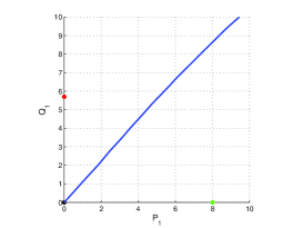
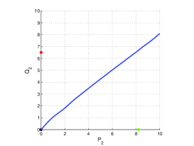
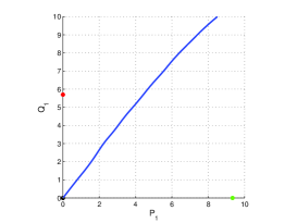
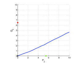
Figure 1: Only population $P$ is able to migrate: separatrix of the basins of attraction of the equilibria $\widehat{E}_{6}$ and $\widehat{E}_{11}$ lying on the axes. The demographic parameters are given by (20). Right column: patch 1; left column: patch 2. Top: $m_{21}=0.1$, $m_{12}=0.1$, $n_{21}=0$, $n_{12}=0$. Bottom: $m_{21}=0.1$, $m_{12}=2.0$, $n_{21}=0$, $n_{12}=0$.

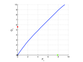
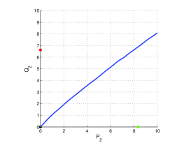
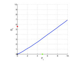
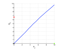
Figure 2: Unidirectional migrations: separatrix of the basins of attraction of the equilibria $\widetilde{E}_{6}$ and $\widetilde{E}_{11}$ lying on the axes. Demographic parameters are given by (20). Right column: patch 1; left column: patch 2. Top: $m_{21}=0.1$, $m_{12}=0$, $n_{21}=0.1$, $n_{12}=0$. Bottom: $m_{21}=2.4$, $m_{12}=0$, $n_{21}=0.1$, $n_{12}=0$.

References

- [1] P.A. Abrams, W.G. Wilson, Coexistence of competitors in metacommunities due to spatial variation in resource growth rates: does predict the outcome of competition?, Ecology Letters 7 (2004) 929–940.
- [2] P. Amarasekare, Coexistence of competing parasitoids on a patchily distributed host: local vs. spatial mechanisms, Ecology 81 (2000) 1286–1296.
- [3] H. Caswell, R.J. Etter, Cellular automaton models for competition in patchy environments: Facilitation, inhibition and tolerance, Bulletin of Mathematical Biology 61 (1999) 615–649.
- [4] R. Cavoretto, S. Chaudhuri, A. De Rossi, E. Menduni, F. Moretti, M. C. Rodi, E. Venturino, Approximation of Dynamical System’s Separatrix Curves, in T. Simos, G. Psihoylos, Ch. Tsitouras, Z. Anastassi (Ed.s), Numerical Analysis and Applied Mathematics ICNAAM 2011 AIP Conf. Proc., 1389 (2011) 1220–1223; doi: 10.1063/1.3637836.
- [5] J. T. Cronin, Movement and spatial population structure of a prairie planthopper, Ecology 84 (2003) 1179–1188.
- [6] C. D. FitzGibbon, Mixed-species grouping in Thomson’s and Grant’s gazelles: the antipredator benefits, Animal Behaviour 39(6) (1990) 1116–1126.
- [7] I. Hanski, Coexistence of competitors in a patchy environment, Ecology 64 (1983) 493–500.
- [8] I. Hanski, Single-species spatial dynamics may contribute to long-term rarity and commonness, Ecology 66 (1985) 335–343.
- [9] I. Hanski, M. Gilpin (Ed.s), Metapopulation biology: ecology, genetics and evolution, London: Academic Press, 1997.
- [10] I. Hanski, A. Moilanen, T. Pakkala, M. Kuussaari, Metapopulation persistence of an endangered butterfly: a test of the quantitative incidence function model, Conservation Biology 10 (1996) 578–590.
- [11] E. P. Hoberg, G. S. Miller, E. Wallner-Pendleton, O. R. Hedstrom, Helminth parasites of northern spotted owls (Strix occidentalis caurina) from Oregon, Journal of Wildlife Diseases 25 (2) (1989) 246–251.
- [12] H.S. Horn, R.H. MacArthur, Competition among fugitive species in a harlequin environment, Ecology 53 (1972) 749–752.
- [13] R. Law, D. Morton, Permanence and assembly of ecological communities, Ecology 77 (1996) 762–775.
- [14] G. Lei, I. Hanski, Metapopulation structure of Cotesia melitaearum, a parasitoid of the butterfly Melitaea cinxia, Oikos 78 (1997) 91–100.
- [15] R. Levins, Some demographic and genetic consequences of environmental heterogeneity for biological control, Bulletin of the Entomological Society America 15 (1969) 237–240.
- [16] J. L. Lockwood, R. D. Powell, M. P. Nott, S. L. Pimm, Assembling in ecologicalcommunities time and space, Oikos 80 (1997) 549–553.
- [17] H. Malchow, S. Petrovskii, E. Venturino, Spatiotemporal patterns in Ecology and Epidemiology, Boca Raton: CRC, 2008.
- [18] J. Mena-Lorca, J. X. Velasco-Hernandez, P. A. Marquet, Coexistence in metacommunities: A three-species model www.ncbi.nlm.nih.gov/pubmed/16964928
- [19] A. Moilanen, I. Hanski, Habitat destruction and competitive coexistence in a spatially realistic metapopulation model, Journal of Animal Ecology 64 (1995) 141–144.
- [20] A. Moilanen, A. Smith, I. Hanski, Long-term dynamics in a metapopulation of the American pika, American Naturalist 152 (1998) 530–542.
- [21] S. Nee, R.M. May, Dynamics of metapopulations: habitat destruction and competitive coexistence, Journal of Animal Ecology 61 (1992) 37–40.
- [22] D. N. Ngoc, R. Bravo de la Parra, M. A. Zavala, P. Auger, Competition and species coexistence in a metapopulation model: Can fast asymmetric migration reverse the outcome of competition in a homogeneous environment?, Journal of Theoretical Biology 266 (2010) 256–263.
- [23] M. Roy, M. Pascual, S.A. Levin, Competitive coexistence in a dynamic landscape, Theoretical Population Biology 66 (2004) 341–353.
- [24] R. L., Schooley, L. C. Branch, Spatial heterogeneity in habitat quality and cross-scale interactions in metapopulations, Ecosystems 10 (2007) 846–853.
- [25] M. Thaker and A.T. Vanak and C.R. Owen and R. Slotow Group dynamics of zebra and wildebeest in a woodland savanna: effects of predation risk and habitat density PLoS One 5(9) e12758, (2010).
- [26] M. Thaker and A.T. Vanak and C.R. Owen and M.B. Ogden and S.M. Niemann and R. Slotow Minimizing predation risk in a landscape of multiple predators: effects on the spatial distribution of African ungulates Ecology 92(2) (2011) 398–407.
- [27] D. Tilman, Competition and biodiversity in spatially structured habitats, Ecology 75 (1994) 2–16.
- [28] M. Valeix, A.J. Loveridge, S. Chamaillé-Jammes, Z. Davidson, F. Murindagomo, H. Fritz, D.W. Macdonald Behavioral adjustments of African herbivores to predation risk by lions: spatiotemporal variations influence habitat use Ecology 90(1), (2009) 23–30.
- [29] E. Venturino, Simple metaecoepidemic models, Bulletin of Mathematical Biology 73 (5), (2011) 917–950.
- [30] J. A. Wiens, Wildlife in patchy environments: metapopulations, mosaics, and management, in D. R. McCullough (Ed.) Metapopulations and Wildlife Conservation, Washington: Island Press, 53–84, 1996.