Signal Estimation from Nonuniform Samples with RMS Error Bound – Application to OFDM Channel Estimation

Abstract

We present a channel spectral estimator for OFDM signals containing pilot carriers, assuming a known delay spread or a bound on this parameter. The estimator is based on modeling the channel’s spectrum as a band-limited function, instead of as the discrete Fourier transform of a tapped delay line (TDL). Its main advantage is its immunity to the truncation mismatch in usual TDL models (Gibbs phenomenon). In order to assess the estimator, we compare it with the well-known TDL maximum likelihood (ML) estimator in terms of root-mean-square (RMS) error. The main result is that the proposed estimator improves on the ML estimator significantly, whenever the average spectral sampling rate is above the channel’s delay spread. The improvement increases with the spectral oversampling ratio.

I Introduction

A basic task in Orthogonal Frequency Division Multiplexing (OFDM) is the estimation of the channel’s spectrum. The so-called pilot-aided channel estimation (PACE) is an efficient method for this task, which consists in first sampling the channel’s spectrum using several pilot carriers, and then interpolating it at the data carrier frequencies [1]. There is a large number of references that discuss this kind of spectral estimation from various points of view, and several surveys [2, 3, 1]. Just to cite some of the relevant approaches, [4] analyzes the ML and the minimum mean-square error (MMSE) estimators. In [5], the authors apply the ESPRIT algorithm to this problem assuming a parametric channel model, and in [6] the estimation method is based on the Singular Value Decomposition. In [7] and [8], the estimation performance is improved by reducing the leakage in the truncation of the channel’s response. In [9], the design of nonuniform pilot distributions is studied. Finally, there exist letters dedicated to specific systems like [10] for DVB-T2.

In PACE, the tapped delay-line (TDL) is the basic analytical tool that allows one to reduce the estimation problem to that of determining the so-called tap weights. However, it has the drawback that the discrete channel’s response must be truncated at some indices, thus introducing a mismatch. This truncation is actually an instance of the well-known Gibbs phenomenon [11]. In order to overcome this drawback, we propose in this letter to model the channel’s spectrum in PACE in an alternative way. Instead of using the TDL model, we propose to first expand the spectrum in a sinc series, and then proceed to minimize the expected root-mean-square (RMS) error assuming a linear estimator. The sinc series in this letter requires knowledge about the channel’s delay spread, a parameter that in practice can be either estimated [12] or at least upper bounded from basic considerations about the propagation channel.

The letter has been organized as follows. In Sec. II, we analyze the basic spectral estimation method in OFDM systems that employ pilot carriers, and present the rationale of the letter. Then, in Sec. III we derive an estimator for a generic band-limited signal from nonuniform samples, in which the performance measure is the RMS error. This estimator will be directly applicable to the problem already discussed in Sec. II through a proper normalization of the channel’s spectrum. Finally, we will present a numerical example in Sec. IV from a well-known reference, in which a channel spectrum is estimated from pilot carriers in an OFDM system. In this example, we will compare the performance of the proposed estimator with that of the ML estimator based on the usual TDL model.

I-A Notation

In this letter, we will employ the following notation:

• New symbols or functions will be introduced using “$\equiv$”.

• Vectors and matrices will be denoted in lower- and upper-case bold font, respectively, ($\mathbf{m}$, $\mathbf{M}$).

• $\mathbf{I}$ will stand for an identity matrix of proper size.

• For a given matrix $\mathbf{A}$ or vector $\mathbf{a}$, $[\mbox{\boldmath$\mathbf{A}$\unboldmath}]_{p,q}$ and $[\mbox{\boldmath$\mathbf{p}$\unboldmath}]_{r}$ will respectively denote the $p,q$ component of $\mathbf{A}$, and the $r$th component of $\mathbf{a}$.

• $\mbox{\boldmath$\mathbf{A}$\unboldmath}^{H}$, $\mbox{\boldmath$\mathbf{A}$\unboldmath}^{T}$ will respectively denote the hermitian and transpose of $\mathbf{A}$.

• ${\mathrm{E}}\{\cdot\}$ will denote the expectation operator.

II Basic channel estimation in OFDM from pilot carriers

Consider a static channel with impulse response ${\mathrm{h}}(t)$ of finite duration, whose support is contained in the range $]0,T_{h}[$. We may view $T_{h}$ as the channel’s delay spread or as an upper bound on this parameter. If the channel’s input is an OFDM signal containing pilot carriers, the problem of estimating the channel’s spectrum can be posed entirely in the frequency domain, once the usual DFT processing has been performed [1, Sec. II]. Basically, after this processing we may assume that $M$ noisy samples $V_{m}$ of the channel’s spectrum ${\mathrm{H}}(f)$ are available at distinct frequencies $f_{m}$ (pilot frequencies). We take this spectrum ${\mathrm{H}}(f)$ as the actual spectrum of the channel, and not as an effective response formed by the channel and the transmit and receive filters. The samples $V_{m}$ follow the model

$$V_{m}={\mathrm{H}}(f_{m})+E_{m},$$ (1)

where $E_{m}$ are independent complex Gaussian noise samples of variance $\sigma_{E}^{2}$. In general terms, the design of a linear estimator in PACE consists in determining a set of coefficients ${\mathrm{g}}_{m}(f)$ such that

$${\mathrm{H}}(f)\approx\sum_{m=1}^{M}{\mathrm{g}}_{m}(f)V_{m},$$ (2)

where the error measure is the expected RMS error given by

$$\Big{(}{\mathrm{E}}\big{\{}\big{|}{\mathrm{H}}(f)-\sum_{m=1}^{M}V_{m}{\mathrm{g}}_{m}(f)\big{|}^{2}\big{\}}\Big{)}^{1/2}.$$ (3)

For obtaining ${\mathrm{g}}_{m}(f)$, the usual approach in the literature consists in approximating ${\mathrm{H}}(f)$ using a TDL model. Specifically, if we truncate an effective discrete response of the channel, we obtain the approximation

$${\mathrm{H}}(f)\approx T\sum_{q=q_{1}}^{q_{2}}h_{e,q}{\mathrm{e}}^{-j2\pi qTf},$$ (4)

where $T$ is the TDL spacing, $h_{e,q}$ are samples of the discrete response, and $q_{1}$ and $q_{2}$ are proper truncation indices. By substituting this formula into (2), we obtain a signal model with a finite number of unknown parameters $h_{e,q}$,

$$V_{m}=T\sum_{q=q_{1}}^{q_{2}}h_{e,q}{\mathrm{e}}^{-j2\pi qTf}+E_{m}.$$ (5)

Finally, if $h_{e,q}$ is identifiable from $V_{m}$, i.e. if $q_{2}-q_{1}+1\leq M$, then we may approximate $h_{e,q}$ using well-known estimators, like the ML or MMSE estimators and, finally, interpolate ${\mathrm{H}}(f)$ using (4), [4, Sec. III]. This is the usual estimation approach in PACE.

Consider now the formula in (4). Its right-hand side is a truncated Fourier series, which is a suitable tool for approximating periodic functions. However, its left-hand side, ${\mathrm{H}}(f)$, is hardly ever periodic in practice. We can see this point by inspecting a typical channel response like

$${\mathrm{h}}(t)=\sum_{k=0}^{K-1}a_{k}\delta(t-\tau_{k}),$$ (6)

for amplitudes $a_{k}$ and delays $\tau_{k}$. Its spectrum

$${\mathrm{H}}(f)=\sum_{k=0}^{K-1}a_{k}{\mathrm{e}}^{-j2\pi\tau_{k}f}$$ (7)

is not $(1/T)$-periodic, unless all the delays $\tau_{k}$ are integer multiples of $T$, a highly unlikely event in practice. The mismatch between the left- and right-hand sides of (4) is no other thing than the well-known Gibbs phenomenon [11]. For channel modeling, this phenomenon is not relevant, given that we may always increase the number of taps in (4), so confining the Gibbs phenomenon to small bands close to the frequencies $\pm 1/(2T)$. However, for estimating the channel’s spectrum using (4), we have that we cannot increase the number of taps without limits, because it must be $q_{2}-q_{1}+1\leq M$ for the coefficients $h_{e,q}$ to be identifiable in (5). So, if we use the TDL interpolator in (4) to reduce the initial model in (1) to that in (5), we have introduced a mismatch. As a consequence, we may expect that statistically efficient estimators for (5), like the ML estimator, do have an additional RMS error component due to this Gibbs phenomenon we have just described.

In order to eliminate this Gibbs phenomenon, we propose in this letter to replace the TDL interpolator in (4) with a description that better suits the properties of channel spectra. In simple terms, we propose to model ${\mathrm{H}}(f)$ as a band-limited function, and describe it using a sinc series. More precisely, since the spectrum of ${\mathrm{H}}(f)$ is contained in $]-T_{h},0[$ we have that the following series is valid:

$${\mathrm{H}}(f)={\mathrm{e}}^{-j\pi fT_{h}}\sum_{p=-\infty}^{\infty}{\mathrm{H}}\Big{(}\frac{p}{T_{h}}\Big{)}(-1)^{p}{\mathrm{sinc}}(fT_{h}-p).$$ (8)

In contrast with the TDL interpolator in (4), this series for ${\mathrm{H}}(f)$ is exact, i.e, there are no truncation errors. There is, however, a technical nuisance that must be taken into account when interpreting (8). The time content of ${\mathrm{h}}(t)$ must lie in $]0,T_{h}[$ and not in $[0,T_{h}]$, because ${\mathrm{H}}(f)$ must be modeled as a bounded function and not as a finite-energy one; (see [13, Sec. 6.8] for this technical difference). This is so because typical channel responses like that in (6) have spectra that cover the whole frequency axis and their energy is, therefore, infinite. Additionally, this alternative modeling of ${\mathrm{H}}(f)$ requires to measure its size using the supremum norm and not the energy. So, we require a bound $A$ such that $|{\mathrm{H}}(f)|\leq A$ for any $f$. This bound will have a theoretical use only, given that it will allow us to derive a proper bound on the estimation error.

We proceed to derive the proposed estimator for ${\mathrm{H}}(f)$ in the next section using a sinc series like (8). The starting point will be the RMS error formula in (3). However, we will perform the derivation for a generic bounded band-limited signal ${\mathrm{s}}(x)$ with spectral support $]-1/2,1/2[$, given that the estimator derived will be usable whenever any signal of this kind (in any application) must be estimated from its own nonuniform samples. The problem addressed in the next section is the following.

Estimation problem.

Consider a bounded band-limited signal ${\mathrm{s}}(x)$, $|{\mathrm{s}}(x)|\leq A$, with spectral support lying in $]-1/2,1/2[$. Also let $z_{m}$ denote $M$ noisy samples following the model

$$z_{m}={\mathrm{s}}(x_{m})+{\mathrm{\epsilon}}_{m},$$ (9)

where the ${\mathrm{\epsilon}}_{m}$ are independent complex Gaussian samples of equal variance $\sigma_{\epsilon}^{2}$ and zero mean, and the abscissas $x_{m}$ are distinct. The objective is to estimate ${\mathrm{s}}(x)$ using a linear estimator with coefficients ${\mathrm{c}}_{m}(x)$, with small error specified by

$$\Big{(}{\mathrm{E}}\big{\{}\big{|}{\mathrm{s}}(x)-\sum_{m=1}^{M}z_{m}{\mathrm{c}}_{m}(x)\big{|}^{2}\big{\}}\Big{)}^{2}.$$ (10)

We view ${\mathrm{s}}(x)$ as deterministic.

This is the problem we have just discussed if we identify the following functions and variables:

$${\mathrm{s}}(x) \;\rightarrow\;{\mathrm{H}}\Big{(}\frac{x}{T_{h}}\Big{)}{\mathrm{e}}^{j\pi x} z_{m} \;\rightarrow\;V_{m}{\mathrm{e}}^{j\pi x_{m}}$$ (11)

$${\mathrm{\epsilon}}_{m} \;\rightarrow\;E_{m}{\mathrm{e}}^{j\pi x_{m}} {\mathrm{c}}_{m}(x) \;\rightarrow\;{\mathrm{e}}^{j\pi(x-x_{m})}{\mathrm{g}}_{m}(x/T_{h})$$

$${\mathrm{x}} \;\rightarrow\;fT_{h}$$

III Design of the signal estimator

Consider the signal ${\mathrm{s}}(x)$ in the previous estimation problem and its sinc series

$${\mathrm{s}}(x)=\sum_{p=-\infty}^{\infty}{\mathrm{s}}(p){\mathrm{sinc}}(x-p).$$ (12)

This series is called Zakai’s series in the sampling theory literature, and it holds due to Theorem 6.21 in [13], where we view the samples ${\mathrm{s}}(p)$ as deterministic and bounded, $|{\mathrm{s}}(p)|\leq A$. Note that the bandwidth of ${\mathrm{s}}(t)$ must be strictly smaller than 1. Actually, there are signals of bandwidth 1, like $\sin(\pi t)$, for which (12) is false. By substituting (9) into (10) and using ${\mathrm{E}}\{\epsilon_{m}\}=0$, we obtain:

$${\mathrm{E}}\{|{\mathrm{s}}(x)-\sum_{m=1}^{M}z_{m}{\mathrm{c}}_{m}(x)|^{2}\}\\ ={\mathrm{E}}\{|{\mathrm{s}}(x)-\sum_{m=1}^{M}({\mathrm{s}}(x_{m})+{\mathrm{\epsilon}}_{m}){\mathrm{c}}_{m}(x)|^{2}\}\\ =|{\mathrm{s}}(x)-\sum_{m=1}^{M}{\mathrm{s}}(x_{m}){\mathrm{c}}_{m}(x)|^{2}+\sigma_{\epsilon}^{2}\sum_{m=1}^{M}|{\mathrm{c}}_{m}(x)|^{2}.$$ (13)

Next, the first term can be bounded using the sinc series in (12), noting that $|{\mathrm{s}}(p)|\leq A$:

$$|{\mathrm{s}}(x)-\sum_{m=1}^{M}{\mathrm{s}}(x_{m}){\mathrm{c}}_{m}(x)|^{2}=|\sum_{p=-\infty}^{\infty}{\mathrm{s}}(p){\mathrm{sinc}}(x-p)\hfill\\ \hfill-\sum_{m=1}^{M}\sum_{p=-\infty}^{\infty}{\mathrm{s}}(p){\mathrm{sinc}}(x_{m}-p){\mathrm{c}}_{m}(x)|^{2}\\ =\Big{|}\sum_{p=-\infty}^{\infty}{\mathrm{s}}(p)\Big{(}{\mathrm{sinc}}(x-p)-\sum_{m=1}^{M}{\mathrm{sinc}}(x_{m}-p){\mathrm{c}}_{m}(x)\Big{)}\Big{|}^{2}\\ \leq A^{2}\sum_{p=-\infty}^{\infty}\Big{|}{\mathrm{sinc}}(x-p)-\sum_{m=1}^{M}{\mathrm{sinc}}(x_{m}-p){\mathrm{c}}_{m}(x)\Big{|}^{2}.$$ (14)

By substituting into (13), we obtain

$${\mathrm{E}}\{|{\mathrm{s}}(x)-\sum_{m=1}^{M}z_{m}{\mathrm{c}}_{m}(x)|^{2}\}\leq\\ A^{2}\sum_{p=-\infty}^{\infty}\Big{|}{\mathrm{sinc}}(x-p)-\sum_{m=1}^{M}{\mathrm{sinc}}(x_{m}-p){\mathrm{c}}_{m}(x)\Big{|}^{2}\\ \hfill+\sigma_{\epsilon}^{2}\sum_{m=1}^{M}|{\mathrm{c}}_{m}(x)|^{2}.$$ (15)

Since we intend to minimize the right-hand side of this inequality, we may assume that ${\mathrm{c}}_{m}(x)$ is real, given that ${\mathrm{sinc}}(x)$ is a real function whenever $x$ is real. Next, we may use the property

$$\sum_{p=-\infty}^{\infty}{\mathrm{sinc}}(y-p){\mathrm{sinc}}(y^{\prime}-p)={\mathrm{sinc}}(y-y^{\prime}),$$ (16)

valid for any $y$ and $y^{\prime}$, to expand the summation’s argument in the second line of (15). After straight-forward manipulations, the right-hand side of (15) can be written as a quadratic form. In matrix notation, we obtain

$${\mathrm{E}}\{|{\mathrm{s}}(x)-\sum_{m=1}^{M}z_{m}{\mathrm{c}}_{m}(x)|^{2}\}\leq\\ A^{2}\Big{(}\mbox{\boldmath$\mathbf{c}$\unboldmath}(x)^{T}\Big{(}\mbox{\boldmath$\mathbf{G}$\unboldmath}+\frac{\sigma^{2}_{\epsilon}}{A^{2}}\mbox{\boldmath$\mathbf{I}$\unboldmath}\Big{)}\mbox{\boldmath$\mathbf{c}$\unboldmath}(x)-2\mbox{\boldmath$\mathbf{c}$\unboldmath}(x)^{T}\mbox{\boldmath$\mathbf{g}$\unboldmath}(x)+1\Big{)},$$ (17)

where

$$[\mbox{\boldmath$\mathbf{G}$\unboldmath}]_{m,m^{\prime}} \equiv{\mathrm{sinc}}(x_{m}-x_{m^{\prime}}), [\mbox{\boldmath$\mathbf{g}$\unboldmath}(x)]_{m} \equiv{\mathrm{sinc}}(x-x_{m}),$$

$$[\mbox{\boldmath$\mathbf{c}$\unboldmath}(x)]_{m} \equiv{\mathrm{c}}_{m}(x),$$

$1\leq m\leq M,\,1\leq m^{\prime}\leq M$. The minimum of this form is attained at the argument

$$\hat{}\mbox{\boldmath$\mathbf{c}$\unboldmath}(x)\equiv\Big{(}\mbox{\boldmath$\mathbf{G}$\unboldmath}+\frac{\sigma^{2}_{\epsilon}}{A^{2}}\mbox{\boldmath$\mathbf{I}$\unboldmath}\Big{)}^{-1}\mbox{\boldmath$\mathbf{g}$\unboldmath}(x)$$ (18)

and the corresponding bound in (17) is

$${\mathrm{E}}\{|{\mathrm{s}}(x)-\sum_{m=1}^{M}z_{m}{\mathrm{c}}_{m}(x)|^{2}\}\\ \leq A^{2}\Bigg{(}1-\mbox{\boldmath$\mathbf{g}$\unboldmath}(x)^{T}\Big{(}\mbox{\boldmath$\mathbf{G}$\unboldmath}+\frac{\sigma^{2}_{\epsilon}}{A^{2}}\mbox{\boldmath$\mathbf{I}$\unboldmath}\Big{)}^{-1}\mbox{\boldmath$\mathbf{g}$\unboldmath}(x)\Bigg{)}.$$ (19)

In summary, if we place the samples $z_{m}$ in a vector $[\mbox{\boldmath$\mathbf{z}$\unboldmath}]_{m}\equiv z_{m}$, we have obtained the following linear estimator for ${\mathrm{s}}(x)$,

$${\mathrm{s}}(x)\approx\mbox{\boldmath$\mathbf{g}$\unboldmath}(x)^{T}\Big{(}\mbox{\boldmath$\mathbf{G}$\unboldmath}+\frac{\sigma^{2}_{\epsilon}}{A^{2}}\mbox{\boldmath$\mathbf{I}$\unboldmath}\Big{)}^{-1}\mbox{\boldmath$\mathbf{z}$\unboldmath}.$$ (20)

The application of the replacements in (11) to this formula yields the desired estimator for ${\mathrm{H}}(f)$.

IV Numerical example

In order to assess the proposed estimator, we proceed to compare it with the deterministic ML estimator based on the TDL model. For implementing this last estimator, we have used the model in [4, Sec. III.A]. We consider the following scenario.

OFDM signal

We employ the OFDM signal in [4, Sec. IV.C] with the following parameters,

• DFT size: 512.

• Number of modulated carriers: 433.

• Number of pilots: $M=28$.

• Indices of pilot carriers: $i_{m}=16m$, $m=0,$ $1,$ $\ldots,$ $M-1$.

• For simplicity, we take the frequency spacing $\Delta f=1$.

Channel model

The usual numerical examples for assessing the RMS error in the literature describe the channel’s response using a tap delay line, whose weights have a specific distribution; (see for example [4]). However, the estimator proposed in this letter has been designed for a specific maximum delay spread $T_{h}$, and this parameter can be hardly obtained from a TDL model. Therefore, to assess the proposed estimator we have generated channel impulse responses with a given maximum time spread $T_{h}$. Specifically, we have used channel impulse responses of the form in (6), where

• $K-1$ has a Poisson distribution of parameter $\lambda=9$.

• $a_{k}$ are independent complex Gaussian variables of zero mean and variance $\sigma_{a}^{2}{\mathrm{e}}^{-2(k-1)/K}$.

• The delays $\tau_{k}$ are uniformly distributed in $[0,T_{h}]$.

• $\sigma_{a}^{2}$ is selected numerically so that

  $${\mathrm{E}}\{|{\mathrm{H}}(f)|^{2}\}=1$$ (21)

  for any $f$.

Signal-to-noise ratio

We define the SNR as

$$\gamma\equiv\frac{{\mathrm{E}}\{|{\mathrm{H}}(f)|^{2}\}}{\sigma_{E}^{2}},$$ (22)

where $\sigma_{E}^{2}$ is the variance of $E_{n}$ in (1). Note that (21) implies $\sigma_{E}^{2}=1/\gamma$. We set $\gamma=30$ dB.

Delay spread

We select the channel duration $T_{h}$ as a function of the pilot average spacing. Specifically, if

$$B_{av}\equiv\frac{i_{M-1}-i_{0}}{M-1}\Delta f,$$ (23)

then we set $T_{h}=\alpha/B_{av}$ for $0\leq\alpha\leq 1$.

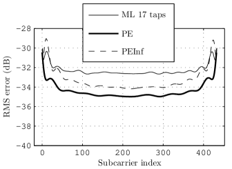
(a) $T_{h}=0.25/B_{av}$

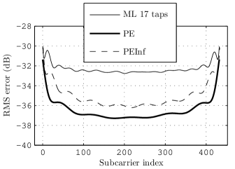
(b) $T_{h}=0.125/B_{av}$

Figure 1: RMS error for the ML, PE, and PEInf estimators.

Figs. 1(a) and 1(b) show the RMS error for $T_{h}=0.25/B_{av}$ and $T_{h}=0.125/B_{av}$, and for the following three estimators:

• ML: ML estimator with the number of taps providing the smallest RMS error.

• PE: Proposed estimator in (20) with the replacements in (11).

• PEInf: This last estimator but setting $\gamma=\infty$.

We can see that estimator PE performs significantly better than estimator ML, and that the improvement is larger for $\alpha=0.125$. In average the improvement is $2.6$ dB and $4.2$ dB for $T_{h}=0.25/B_{av}$ and $T_{h}=0.125/B_{av}$, respectively. Estimator PEInf also outperforms estimator ML, though with a somewhat larger RMS error.

Fig. 2 shows the reduction in RMS error of the estimator PE relative to the estimator ML. For each possible delay $\tau$, we can see in this figure the reduction in RMS error brought by estimator PE at frequency $f$ when the channel is ${\mathrm{h}}(t)=\delta(t-\tau)$. Except at the limit delays and frequencies, the reduction in RMS error is 2.4 dB roughly.

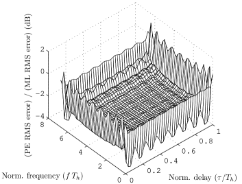
Figure 2: RMS error of proposed method relative to RMS error of TDL estimator for all possible delays and frequencies.

V Conclusions

We have recalled the problem of estimating a channel spectrum from a finite number of nonuniform samples. This problem appears in OFDM system equipped with pilot carriers, after the usual DFT processing. We have shown that this problem can be cast as that of estimating a band-limited signal from nonuniform samples through a proper normalization. Afterward, we have derived an estimator in which the performance measure is the RMS error, assuming that the signal (or channel spectrum) is bounded and the samples are contaminated by independent zero-mean complex Gaussian noise samples of equal variance. Finally, we have compared this estimator with the usual ML estimator based on a TDL model, in order to assess its performance in a basic OFDM setting. The main conclusion is that the proposed estimator improves on the ML estimator in RMS error significantly, provided there is some spectral oversampling.

References

- [1] T. Hwang, C. Yang, G. Wu, S. Li, G. Li, OFDM and its wireless applications: A survey, Vehicular Technology, IEEE Transactions on 58 (4) (2009) 1673–1694.
- [2] L. Tong, B. Sadler, M. Dong, Pilot-assisted wireless transmissions: general model, design criteria, and signal processing, Signal Processing Magazine, IEEE 21 (6) (2004) 12–25.
- [3] M. Ozdemir, H. Arslan, Channel estimation for wireless OFDM systems, Communications Surveys Tutorials, IEEE 9 (2) (2007) 18–48.
- [4] M. Morelli, U. Mengali, A comparison of pilot-aided channel estimation methods for OFDM systems, Signal Processing, IEEE Transactions on 49 (12) (2001) 3065–3073.
- [5] B. Yang, K. Letaief, R. Cheng, Z. Cao, Channel estimation for OFDM transmission in multipath fading channels based on parametric channel modeling, Communications, IEEE Transactions on 49 (3) (2001) 467–479.
- [6] O. Edfors, M. Sandell, J.-J. van de Beek, S. Wilson, P. Borjesson, OFDM channel estimation by singular value decomposition, Communications, IEEE Transactions on 46 (7) (1998) 931–939.
- [7] X. Xiong, B. Jiang, X. Gao, X. You, DFT-based channel estimator for OFDM systems with leakage estimation, Communications Letters, IEEE 17 (8) (2013) 1592–1595.
- [8] J. Seo, S. Jang, J. Yang, W. Jeon, D.-K. Kim, Analysis of pilot-aided channel estimation with optimal leakage suppression for OFDM systems, Communications Letters, IEEE 14 (9) (2010) 809–811.
- [9] P. Fertl, G. Matz, Channel estimation in wireless OFDM systems with irregular pilot distribution, IEEE Trans. on Signal Processing 58 (6) (2010) 3180–3194.
- [10] M. Yu, P. Sadeghi, A study of pilot-assisted OFDM channel estimation methods with improvements for DVB-T2, Vehicular Technology, IEEE Transactions on 61 (5) (2012) 2400–2405.
- [11] D. Gottlieb, C.-W. Shu, On the gibbs phenomenon and its resolution, SIAM Rev. 39 (4) (1997) 633–668.
- [12] C. R. N. Athaudage, A. D. S. Jayalath, Delay-spread estimation using cyclic-prefix in wireless OFDM systems, Communications, IEE Proceedings- 151 (6) (2004) 559–566.
- [13] J. R. Higgins, Sampling Theory in Fourier and signal analysis. Foundations., 1st Edition, Oxford Science Publications, 1996.