RingFinder: automated detection of galaxy-scale gravitational lenses
in ground-based multi-filter imaging data

Abstract

We present RingFinder, a tool for finding galaxy-scale strong gravitational lenses in multi-band imaging data. By construction, the method is sensitive to configurations involving a massive foreground early-type galaxy and a faint, background, blue source. RingFinder detects the presence of blue residuals embedded in an otherwise smooth red light distribution by difference imaging in two bands. The method is automated for efficient application to current and future surveys, having originally been designed for the 150-deg2 Canada France Hawaii Telescope Legacy Survey (CFHTLS). We describe each of the steps of RingFinder. We then carry out extensive simulations to assess completeness and purity. For sources with magnification $\mu>$4, RingFinder reaches 42% (resp. 25%) completeness and 29% (resp. 86%) purity before (resp. after) visual inspection. The completeness of RingFinder is substantially improved in the particular range of Einstein radii $0\farcs 8\leq R_{\rm Ein}\leq 2\farcs 0$ and lensed images brighter than $g=22.5$, where it can be as high as $\sim$70%. RingFinder does not introduce any significant bias in the source or deflector population. We conclude by presenting the final catalog of RingFinder CFHTLS galaxy-scale strong lens candidates. Additional information obtained with Hubble Space Telescope and Keck Adaptive Optics high resolution imaging, and with Keck and Very Large Telescope spectroscopy, is used to assess the validity of our classification, and measure the redshift of the foreground and the background objects. From an initial sample of 640,000 early type galaxies, RingFinder returns 2500 candidates, which we further reduce by visual inspection to 330 candidates. We confirm 33 new gravitational lenses from the main sample of candidates, plus an additional 16 systems taken from earlier versions of RingFinder. First applications are presented in the SL2S galaxy-scale Lens Sample paper series.

1 Introduction

Since the discovery of the first multiple quasar produced by strong gravitational lensing by a foreground massive galaxy (Walsh et al. 1979), and the discovery of the first giant arcs found at the centers of galaxy clusters (Soucail et al. 1987; Lynds & Petrosian 1986), much progress has been made in exploiting the unique capabilities of strong gravitational lensing as a probe of the mass content of distant massive objects, independent of the nature of their constituents or their dynamical state. With the advent of deep, wide-field optical imaging surveys we have now entered a new era that enables the use of sizable samples of strong lensing events as precision diagnostics of the physical properties of the distant Universe.

Gravitational lensing, by itself and in combination with other probes, can be used to great effect to measure the mass profiles of early-type galaxies, both in the nearby universe and at cosmological distances (e.g.  Treu & Koopmans 2002a, b; Rusin et al. 2003; Treu & Koopmans 2004; Rusin & Kochanek 2005; Koopmans et al. 2006; Jiang & Kochanek 2007; Gavazzi et al. 2007; Treu 2010; Auger et al. 2010; Lagattuta et al. 2010; Sonnenfeld et al. 2012; Bolton et al. 2012; Dye et al. 2013; Oguri et al. 2013). Until recently, however, this approach was severely limited by the small size of the samples of known strong gravitational lenses. This has motivated a number of dedicated searches which have increased the sample of known strong gravitational lens systems by more than an order of magnitude in the past decade.

Different search strategies have been adopted depending on the properties of the parent survey. A fundamental distinction is that between source-oriented and deflector-oriented searches (e.g. Schneider et al. 1992). The choice depends on the relative abundance of the population of foreground deflectors and that of background sources, and has strong implications for the potential applications of the resulting lens catalog.

Historically, source-oriented surveys were considered first, as they generally require the analysis of a relatively small input catalog of magnified sources that turn out to be much brighter than the foreground deflector at a carefully chosen wavelength. The sources of choice were typically bright quasars or radiosources, that would outshine the light from the deflector. This approach is well-illustrated in the optical by the Sloan Quasar Lens Survey (SQLS Inada et al. 2003, 2012), the near IR with MUSCLES (Jackson et al. 2012), and in the radio by the Cosmic Lens All Sky Survey (CLASS) (Myers et al. 2003; Browne et al. 2003). This last survey led to the early discovery of 22 gravitationally lensed quasars, many of which have been followed up with HST . The latest release of the SQLS lens catalog has reported the discovery of 49 new quasar lenses. The scarcity of the population of background sources ($\sim 0.1$ per deg², Oguri & Marshall 2010) requires extremely wide field surveys in order to gather sizable lens samples.

Recently, wide field imaging surveys at millimeter wavelengths with the South Pole Telescope (SPT, Hezaveh et al. 2013), and sub-millimeter wavelengths with the Herschel satellite like H-ATLAS (Negrello et al. 2010; González-Nuevo et al. 2012; Bussmann et al. 2013) and HerMES (Conley et al. 2011; Gavazzi et al. 2011; Wardlow et al. 2013), have made it possible to target the population of distant sub-mm galaxies in the redshift range $1-4$ and find large number of lenses, a result predicted by Blain (1996).

These surveys lead to a spatial density of strong lenses ranging between 0.1 and 0.2 deg^-2 (Negrello et al. 2010; Wardlow et al. 2013; Vieira et al. 2013). The recent availability of high-resolution spectro-imaging with the Atacama Large Millimeter Array (ALMA) of gravitational lenses found at those wavelengths makes this technique a very promising avenue for the coming decade (Hezaveh et al. 2013). We expect that a similar density of lensed quasars will be reached by optical surveys as well, including the Dark Energy Survey, the HSC Survey and in the next decade LSST and Euclid (Oguri & Marshall 2010).

Indeed, at optical wavelengths, where unobscured star-forming galaxies are clearly visible, the ever-increasing deep wide field imaging and spectroscopic surveys are providing a population of distant background sources that has reached several hundreds of thousands per square degree. Since these are generally much fainter than the foreground massive early type galaxy deflectors, an effective strategy is to focus on these less numerous foreground galaxies and look for signatures of a gravitationally-lensed background object. As most of these background sources are spatially resolved, they take the typical shape of a complete, or partial, arc-like, Einstein ring. The challenge of this approach generally resides in the limited spatial resolution of wide field surveys, and the somewhat similar wavelengths at which both the lens and the source shine, which makes it difficult to disentangle the source and deflector light.

A particularly successful way to mitigate this problem has been to take advantage of large spectroscopic surveys, such as the Sloan Digital Sky Survey (SDSS), which took spectra of several hundreds of thousands of bright galaxies. By looking for composite spectra consisting of two objects at different redshifts within the solid angle covered by the spectroscopic fiber, it has been possible to build a large sample of galaxy-galaxy lens systems. These consist typically of a low redshift foreground massive early-type galaxy and a background star-forming galaxy at higher redshift. The Sloan Lens ACS Survey (SLACS) conducted HST follow-up observations of such spectroscopic candidates, and discovered about 100 gravitational lenses in the redshift range $0.1\leq z_{\rm d}\leq 0.4$ (Bolton et al. 2004, 2006; Auger et al. 2010). Rarer configurations, involving a foreground late-type galaxy, or a background early-type galaxy, were also searched for (Treu et al. 2011; Brewer et al. 2012; Auger et al. 2011). Recently, this technique has been extended to the SDSS-III survey and has been used to find more lenses at $z\lesssim 0.6$ (Brownstein et al. 2012; Bolton et al. 2012). The main advantage of this spectroscopic approach is that important quantities, such as the deflector and source redshifts along with the velocity dispersion of the stars in the deflector, are obtained from the parent survey itself. The availability of this data allows for many scientific applications including, combined lensing+dynamical studies of these systems (Treu & Koopmans 2004; Koopmans et al. 2006, 2009; Auger et al. 2010; Sonnenfeld et al. 2012), without the need for targeted spectroscopic follow-up.

Even though the approaches described above have been very successful, there is strong motivation to develop techniques to identify galaxy-galaxy lenses purely in imaging data. This is challenging, but it can potentially yield a larger number of objects than any other technique: Marshall et al. (2005) forecast more than 10 such systems per square degree at HST -like depth and resolution. Similar numbers are expected for Euclid/LSST. We therefore expect an all-sky survey should find more than $10^{5}$ such systems. Finding a similar sample of systems from an all-sky spectroscopic catalog would require of order $10^{8}$ spectra, two orders of magnitude more than have been taken to date.

Because of the difficulty of identifying galaxy-galaxy lenses in optical images, much effort has been devoted to the analysis of HST data in order to exploit its resolution. Searches based on both visual and automated inspection have been conducted (e.g. Ratnatunga et al. 1999; Moustakas et al. 2007; Faure et al. 2008; Jackson 2008; Marshall et al. 2009; Pawase et al. 2012; Newton et al. 2009), yielding several tens of candidates over the few square degrees of available data.

Still, ground-based imaging is a potentially promising avenue, with its relatively low angular resolution compensated by the ready availability of hundreds or thousands of square degrees in multiple bands. In the SDSS, with typically $1\farcs 5$ seeing and limiting magnitude $r\sim 21.5$, only wide separation systems produced by very massive galaxies, groups or clusters of galaxies have been able to be uncovered (Belokurov et al. 2009). The success rate increases significantly with angular resolution, and therefore sub-arcsecond image quality is desirable. Thus, good image quality and wide area coverage, such as that provided by the Canada France Hawaii Legacy Survey (CFHTLS), are potentially more promising sources of lenses – especially those with deflector redshifts $\sim 0.5$ and above, where current samples are scant (Treu et al. 2010). This argument motivated the Strong Lensing Legacy Survey (SL2S), which comprised a search for group and cluster scale (Einstein Radius $R_{\rm Ein}\gtrsim 3\arcsec$) lenses (Cabanac et al. 2007; More et al. 2012), and the present work, the SL2S galaxy-scale lens search. The ultimate goal of our work was to use the newly found lenses to study the formation and evolution of massive galaxies; our results can be found in Ruff et al. (2011); Gavazzi et al. (2012); Sonnenfeld et al. (2013a, b).

In this paper we present RingFinder, the semi-automated procedure for finding galaxy-scale strong lenses in the multi-band imaging data that we have applied to the CFHTLS. By focusing on the most frequent lens-source configuration, that of a foreground red massive early-type galaxy and a faint blue background source at higher redshift, we implement a technique that subtracts off the foreground light and analyses the blue residuals by requiring that they are broadly consistent with a strong lensing event. The CFHTLS data are described in Section 2 while Section 3 describes the RingFinder algorithm. A list of 330 lens candidates, plus 71 additional candidates from preliminary versions of RingFinder and additional datasets are also presented in this section.

In Section 4 we describe the extensive and realistic simulations of plausible galaxy-scale lens systems which we use to assess the performance of the method, both in terms of completeness and purity. We explore the dependence of those quantities on important parameters like the Einstein radius, source magnitude, and lens and source redshifts in order to characterize the selection function of the RingFinder sample.

Then, in Section 5 we summarize the results of our multi-year follow-up campaign with high resolution imagers and spectrographs, present the sample of confirmed lenses, and discuss false positives and contaminants. We summarize our main results and present our conclusions in Section 6.

Throughout this paper, all magnitudes referred to are calculated in the AB system, and we assume the concordance $\Lambda$CDM cosmological background with $\Omega_{\rm m}=0.3$, $\Omega_{\Lambda}=0.7$ and $H_{0}=70$ km s^-1 Mpc^-1.

2 The CFHT Legacy Survey

The Canada-France-Hawaii Telescope Legacy Survey (CFHTLS) is a major photometric survey of more than 450 nights over 5 years (started on June 1st, 2003) using the MegaCam wide field imager which covers $\sim$1 square degree on the sky, with a pixel size of 0$\farcs$186. The CFHTLS has two components aimed at extragalactic studies: a Deep component consisting of 4 pencil-beam fields of 1 deg² and a Wide component consisting of 4 mosaics covering 150  deg² in total. Both surveys are imaged through 5 broadband filters. The data are pre-reduced at CFHT with the Elixir pipeline which removes the instrumental artifacts in individual exposures. The CFHTLS images are then astrometrically calibrated, photometrically inter-calibrated, resampled and stacked by the Terapix group at the Institut d’Astrophysique de Paris (IAP) and finally archived at the Canadian Astronomy Data Centre (CADC). Terapix also provides weight map images, quality assessments meta-data for each stack as well as mask files that mask saturated stars and defects of each image. The production of photometric catalogs was made at Terapix using SExtractor (Bertin & Arnouts 1996). In this paper we use the sixth data release (T0006) described in detail by (Goranova et al. 2009)

The Wide survey is a single epoch imaging survey, covering some 150 deg² in 4 patches of the sky. It reaches a typical depth of $u^{*}\simeq 25.35$, $g\simeq 25.47$, $r\simeq 24.83$, $i\simeq 24.48$ and $z\simeq 23.60$ (AB mag of 80% completeness limit for point sources) with typical FWHM point spread functions of $0\farcs 85$, $0\farcs 79$, $0\farcs 71$, $0\farcs 64$ and $0\farcs 68$, respectively. Because of the greater solid angle, the Wide component is our main provider of lens candidates and, unless otherwise stated, the analysis below refers to the application of RingFinder to the Wide survey.

Regions around the halo of bright saturated stars, near CCD defects or near the edge of the fields have lower quality photometry and are discarded from the analysis. Overall, we reject $\sim 21\%$ of the CFHTLS Wide survey area, reducing the total area analyzed in this work to 135.2 deg².

3 The RingFinder pipeline

In this section we present the methodology that we adopted to uncover gravitational lenses in multi-filter imaging data. It is a lens-oriented strategy in the sense that we first select bright early-type galaxies (ETGs) as they presumably are the most massive objects and thus the most efficient gravitational lenses. Then, the bulk of the deflector light is removed by subtracting a scaled version of the $i$-band image from the $g$-band image. Finally, we look for blue features consistent with being gravitationally lensed objects in the residuals.

3.1 Population of foreground Early-Type Galaxies

The starting point of our procedure is a photometric catalog of ETGs that we restrict to a maximum apparent magnitude $17<i<22$ to select the more massive systems in the redshift range more favorable for lensing $(0.2\lesssim z\lesssim 1)$. We take advantage of a version of photometric redshift measurements for the T06 CFHTLS data release updated by the work of Coupon et al. (2009) previously done for T04 earlier data release. These were obtained using LePhare code. The reliability of photometric redshifts has been extensively assessed against spectroscopic redshifts (Ilbert et al. 2006; Coupon et al. 2009). We define our sample of ETGs as those galaxies having a best fit photometric template Spectral Energy Distribution (SED) type $T<22$, corresponding to an SED of an E/SO galaxy. The typical redshift uncertainty for these galaxies down to $22$ is about $0.026$ with only 1.3% of catastrophic failures. We also exclude low redshift $z<0.1$ objects that are too close for being efficient lenses and for which SED fitting leads to greater redshift and type errors, given our filter coverage.

When looking for lenses, however, simple color cuts are not sufficient to obtain complete samples of deflectors. A bright and blue strongly lensed background source can alter significantly the colors of the foreground deflector, misleading the classifier to think it is of a different spectral type. In order not to miss some of the potentially more promising targets we have thus augmented our sample of red galaxies in the following fashion (A fully quantitative justification of this procedure is given in Section 4.4.4 with the aid of our extensive simulations).

We measure colors $(g-i)_{\rm in}$ and $(g-i)_{\rm out}$ in two concentric circular apertures $R_{\rm in}=1\farcs 86$ and $R_{\rm out}=3\farcs 35$ and we add to our catalog of potential lensing ETGs all galaxies that have a red core and have a substantially bluer envelope regardless of their best fit SED template type $T$. The criteria are as follow:

$$(g-i)_{\rm in} > 1.4$$

$${\rm and}$$

$$(g-i)_{\rm in}-(g-i)_{\rm out} < 0.2\;.$$ (2)

As we show later these cuts are sufficient to add all the interesting targets. With this supplement, we typically end up with 3740 target ETGs per sq. degree (20% of which have a substantial color gradient). We are therefore left with $\sim 638\,000$ objects. Their photometric redshift distribution along with their $(g-i)_{\rm ETG}$ color as a function of redshift is shown in Fig. 1. The median redshift is $z_{\rm med}=0.58$ with 16th and 84th percentiles of 0.36 and 0.82, respectively. This suggests that this parent dataset should be excellent for identifying a sample of gravitational lenses with deflector redshift $z>0.4$, and hence complement lower redshift samples like the SLACS.

Figure 1: Top panel: redshift distribution of Early-Type Galaxies in the CFHTLS Wide down to a magnitude of $i<22$. Bottom panel: mean (solid) and standard deviation (dashed) of the $(g-i)_{\rm ETG}$ color variation as a function of redshift.

3.2 $g-\alpha\,i$ difference imaging

For simplicity we approximate ETGs as having the same shape and radial light profile in both $g$ and $i$ bands (we will justify this choice below). With this approximation, lensed features that have different colors than the deflector will show up in $g-\alpha\ i$ difference images, where $\alpha$ is an appropriate scaling factor. As we will see, this approximation allows us to remove the foreground deflector light robustly and with sufficient precision to identify background lensed features as positive residuals with blue colors.

3.2.1 PSF matching and subtraction

As a first step we have to match the spatial resolution of the red and blue images. To achieve this, we simply convolve the red image with the blue PSF, and vice-versa. Even though it entails some loss of information, this process has the advantage of being robust provided we have a good control of PSF variations over the large Megacam 1 deg² field-of-view. To understand the PSF, we build catalogs of bright unsaturated stars in the magnitude range $17.3<i<21$ for each CFHTLS pointing. For each ETG, we look for all the neighboring stars less distant than 4 arcmin, align them with sub-pixel accuracy and make a flux-weighted average in each of the $g$ and $i$ bands. In most cases the image subtraction for ETGs leaves us with very small residuals down to a radius of $\sim 0\farcs 5$. On smaller scales, imperfect PSF matching and/or some unaccounted-for color gradient or nuclear emission prevents us from reaching residuals consistent with noise. We thus conservatively discard residuals on scales below $0\farcs 6$. This effectively sets a lower limit to the Einstein Radius of the gravitational lens systems that can be identified by RingFinder.

The two light distributions are then matched by optimizing the value of the scaling parameter $\alpha$ using a linear regression of the $g$ and $i$ pixel values in the aperture $0\farcs 5\leq R\leq 2\arcsec$. We then repeat a symmetric 3-sigma clipping of discrepant pixels four times to end up with a $(g-i)$ color index map in which the deflector light is suppressed.

3.2.2 Deflector light profile analysis

We use the sigma-clipped pixels described in the previous section to perform a simple analysis of the red light distribution. In this process we measure relevant quantities of the ETG, such as the second order moments, axis ratio $q_{\rm L}$, orientation $\theta_{\rm l}$, effective radius $R_{\rm eff,L}$ and Sérsic index $n_{\rm L}$ (Sersic 1968). Even though these quantities are affected by the PSF blurring, they are useful to further refine the pre-selection of ETGs by discarding spurious stars and red spirals. In particular, by discarding the $\sim$12.5% most elongated objects with $q_{\rm L}<0.7$ and deflector having a Sérsic index $n<1.5$, we exclude disky foreground objects for which the assumption of an homogeneous color is poor and will give rise to numerous false positives.

3.2.3 Detection and analysis of residuals

In order to identify significant residuals, we measure the noise level in the $g-\alpha\ i$ color map. We then define a detection by requiring a signal-to-noise-ratio $\nu>1.2$ over at least 10 connected pixels in the unmasked image, provided that the center of light is in the annulus $R_{\rm min}=0\farcs 5\leq R\leq R_{\rm max}=2\farcs 7$. For each such connected region we infer the shape from the zeroth, first and second order moments measured in the area defined by the isophotal detection threshold. In particular, for each connected region we measure a flux $F_{\rm res}$, principal axes $a_{\rm res}$ and $b_{\rm res}$ and their ratio $q_{\rm res}$, the radial separation $R_{\rm res}$, and orientation $\varphi_{\rm res}$ of the main axis with respect to the center of the deflector, and the isophotal area $\mathcal{A}_{\rm res}$. We also keep track of the multiplicity $\mathcal{M}$ of the residual, i.e. whether we detect several residuals around a given foreground ETG.

Detections with width $b_{\rm res}<0\farcs 2$ are considered spurious given the typical image quality in both the $g$ and $i$ bands. After this step, we find that about 14370 ETGs exhibit one or more detectable blue residuals. Given the 135.2 deg² effective area, this corresponds to about 106 objects per square degree. We also readily see that about 97.7% of the parent population of ETGs isolated in §3.1 are automatically removed by our automated RingFinder pipeline.

However at this stage we have not yet taken advantage of the measured quantities like $F_{\rm res}$, $q_{\rm res}$, $R_{\rm res}$ and $\varphi_{\rm res}$ which as we will show will help further select actual lens candidates and eliminate false positives. As justified by the simulations presented in §4 and the association of previously known lenses, we apply the following cuts:

• the orientation of the major axis of the residual should be nearly tangential with respect to the center of the deflector. This reads $|\varphi|\leq 30^{\circ}$.

• the flux $F_{\rm res}$ should correspond to an AB magnitude $m_{\rm res}\leq 25.5$, the area $\mathcal{A}_{\rm res}<7$ arcsec² and the mean surface brightness $<26.3$ mag/arcsec².

• If one and only one residual is found ($\mathcal{M}=1$), then we require it to be elongated $q_{\rm res}<0.7$. Otherwise, if $\mathcal{M}\geq 2$, the object is considered in the catalog of lens candidates.

After these cuts aiming at maximizing the recovery rate, we end up having 2524 lens candidates passing all these automatic criteria, corresponding to a spatial density of about 18 deg^-2.

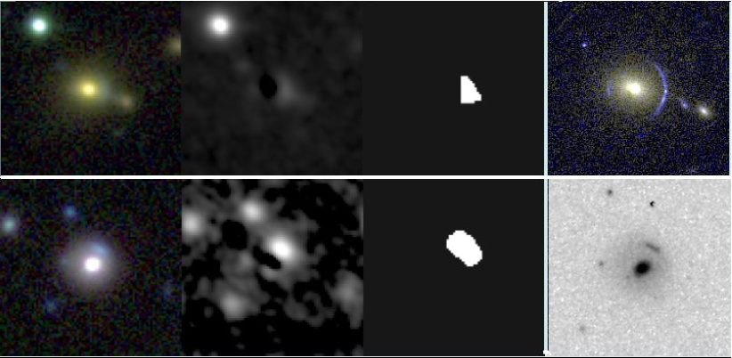
Figure 2: Two examples of RingFinder outputs. The first column is a gri composite color image. The second column shows the result of the $g-\alpha i$ difference imaging that performs well at suppressing the deflector light and picking the blue arc-like residuals. The third column shows the detected area(s) and the forth column shows the HST counterpart. Images are 15 arcsec on a side. In the first row we see a good candidate in a typical cusp configuration where only the bright outer image is detected. The second row illustrates a typical false positive consisting of a nearly face-on disky galaxy with a prominent bulge.

3.3 Visual inspection

These 2524 candidates were subsequently visually scrutinized by the authors in order to identify obvious spurious objects and refine our lensing classification. We thus defined a quality factor called q_flag taking 4 possible values, 0: not a lens, 1: possibly a lens, 2: probably a lens, 3: definitely a lens. The classification is similar to the scheme adopted for the SLACS survey (Bolton et al. 2004, 2006; Auger et al. 2009). The visual classification is very fast as the 2524 candidate lensing ETGs could be visualized and classified in a few hours for a single individual. When the eyeball classification of the authors disagreed, a consensus classification for each object was achieved via a short discussion.

The visual classification criteria are somewhat subjective as they rely on the experience of the authors in observing, simulating, and modeling confirmed lenses. It is an iterative process that builds on the existence of some high resolution HST imaging of the COSMOS field whose intersection with the CFHTLS deep field is one square degree and in which a sample of gravitational lenses was published (Faure et al. 2008; Jackson 2008). In addition, as explained below, some early follow up imaging with HST allowed us to train our classification. Figures like in Fig. 2 were produced for known lenses to see how they would look like and to know what to expect. It is not trivial to figure out that the first row is an actual lens whereas the second one is a nearly pole-on view of a disky galaxy with a prominent bulge and a bright arm in the disk.Note that RingFinder yields very similar outputs for the three objects shown in the figure. This illustrates that it will be difficult to circumvent the need of a final informed visual inspection, or the need for follow-up for final confirmation.

The visualization step allowed us to select 330 good and medium quality lens candidates that are presented and further investigated in §5. They are listed in table 3.3.

Table 1: The SL2S galaxy-scale main sample of lens candidates in the CFHTLS-Wide.

name SL2SJ…	RA	DEC	magi	$z_{\rm phot,d}$	$z_{\rm d}$	$z_{\rm s}$	q_flag	confirmed
020457$-$110309	31.2392	-11.0526	19.91	0.756	0.609	1.888	3	3
020524$-$093023	31.3527	-9.5065	19.46	0.697	0.557	1.335	3	3
020904$-$055529	32.2708	-5.9247	18.59	0.451	$\cdots$	$\cdots$	3	$\cdots$
021206$-$075528	33.0273	-7.9245	19.04	0.494	0.460	$\cdots$	3	2
021233$-$061210	33.1411	-6.2028	18.22	0.452	$\cdots$	$\cdots$	3	$\cdots$
021247$-$055552	33.1993	-5.9312	20.46	0.806	0.750	2.740	3	3
021411$-$040502	33.5467	-4.0841	19.88	0.740	0.609	1.880	3	3
021517$-$061741	33.8222	-6.2948	18.06	0.388	$\cdots$	$\cdots$	3	$\cdots$
021539$-$061918	33.9152	-6.3218	19.43	0.452	$\cdots$	$\cdots$	3	$\cdots$
021737$-$051329	34.4049	-5.2248	19.63	0.856	0.646	1.850	3	3
021801$-$080247	34.5053	-8.0465	20.45	1.058	0.928	2.060	3	3
021902$-$082934	34.7589	-8.4930	18.98	0.499	0.389	2.160	3	3
022046$-$094927	35.1919	-9.8244	19.93	0.603	0.572	2.606	3	3
022056$-$063934	35.2358	-6.6595	18.08	0.389	0.330	$\cdots$	3	3
022346$-$053418	35.9423	-5.5718	18.82	0.546	0.499	1.440	3	3
022357$-$065142	35.9914	-6.8619	18.89	0.511	0.473	1.430	3	3
022708$-$065445	36.7866	-6.9125	20.24	0.693	0.560	1.644	3	3
023238$-$044948	38.1609	-4.8301	18.61	0.374	$\cdots$	$\cdots$	3	$\cdots$
023307$-$043838	38.2794	-4.6440	19.62	0.786	0.671	1.869	3	3
084934$-$043352	132.3926	-4.5646	18.59	0.395	0.373	2.400	3	2
085019$-$034710	132.5795	-3.7863	19.50	0.333	0.337	3.250	3	3
085503$-$023607	133.7648	-2.6020	20.39	0.679	0.622	0.351	3	0
085540$-$014730	133.9172	-1.7918	19.57	0.425	0.365	3.390	3	3
085559$-$040917	133.9996	-4.1549	18.90	0.450	0.419	2.950	3	3
085831$-$035230	134.6317	-3.8751	19.60	0.750	$\cdots$	$\cdots$	3	$\cdots$
135854+560349	209.7272	56.0639	18.88	0.594	0.499	$\cdots$	3	$\cdots$
135949+553550	209.9567	55.5973	20.85	0.887	0.783	2.770	3	3
140123+555705	210.3466	55.9515	19.06	0.639	0.527	$\cdots$	3	3
140156+554446	210.4849	55.7463	18.70	0.504	0.464	$\cdots$	3	3
140454+520024	211.2269	52.0068	17.88	0.490	0.456	1.590	3	3
140533+550231	211.3910	55.0420	19.54	0.793	$\cdots$	$\cdots$	3	3
140614+520253	211.5594	52.0482	18.54	0.510	0.480	$\cdots$	3	2
140845+514913	212.1906	51.8205	19.65	0.739	$\cdots$	$\cdots$	3	$\cdots$
141137+565119	212.9043	56.8553	18.74	0.415	0.322	1.420	3	3
142059+563007	215.2494	56.5021	18.76	0.430	0.483	3.120	3	3
142432+550019	216.1354	55.0055	19.39	0.451	$\cdots$	$\cdots$	3	0
143341+512351	218.4209	51.3978	18.23	0.374	$\cdots$	$\cdots$	3	$\cdots$
220329+020518	330.8709	2.0886	19.37	0.380	0.400	2.150	3	3
221417+011855	333.5723	1.3154	19.99	0.510	$\cdots$	$\cdots$	3	$\cdots$
221852+014038	334.7193	1.6775	19.24	0.612	0.564	$\cdots$	3	2
222148+011542	335.4534	1.2619	18.35	0.346	0.325	2.350	3	3
222217+001202	335.5735	0.2008	19.13	0.421	0.436	1.360	3	3
020049$-$100048	30.2043	-10.0135	21.70	0.969	$\cdots$	$\cdots$	2	$\cdots$
020103$-$034905	30.2666	-3.8181	20.54	0.724	$\cdots$	$\cdots$	2	$\cdots$
020107$-$041845	30.2833	-4.3127	19.47	0.413	$\cdots$	$\cdots$	2	$\cdots$
020148$-$084020	30.4510	-8.6723	19.61	0.476	$\cdots$	$\cdots$	2	$\cdots$
020150$-$065235	30.4608	-6.8766	19.81	0.701	$\cdots$	$\cdots$	2	$\cdots$
020150$-$103811	30.4608	-10.6366	18.78	0.529	$\cdots$	$\cdots$	2	$\cdots$
020152$-$041103	30.4678	-4.1842	20.20	0.897	$\cdots$	$\cdots$	2	$\cdots$
020201$-$063540	30.5049	-6.5945	18.81	0.418	$\cdots$	$\cdots$	2	$\cdots$
020208$-$102006	30.5353	-10.3351	19.99	0.463	$\cdots$	$\cdots$	2	$\cdots$
020232$-$071803	30.6355	-7.3009	19.84	0.463	$\cdots$	$\cdots$	2	$\cdots$
020242$-$082113	30.6764	-8.3537	19.36	0.513	$\cdots$	$\cdots$	2	$\cdots$
020308$-$100941	30.7845	-10.1616	19.71	0.368	$\cdots$	$\cdots$	2	$\cdots$
020328$-$065719	30.8688	-6.9555	20.22	0.735	$\cdots$	$\cdots$	2	$\cdots$
020338$-$051901	30.9097	-5.3171	18.77	0.432	$\cdots$	$\cdots$	2	$\cdots$
020341$-$074722	30.9223	-7.7897	18.73	0.452	$\cdots$	$\cdots$	2	$\cdots$
020342$-$035331	30.9269	-3.8920	18.79	0.289	$\cdots$	$\cdots$	2	$\cdots$
020347$-$111201	30.9476	-11.2003	20.90	0.922	$\cdots$	$\cdots$	2	$\cdots$
020353$-$100703	30.9739	-10.1176	20.37	0.562	$\cdots$	$\cdots$	2	$\cdots$
020404$-$071418	31.0208	-7.2386	19.87	0.382	$\cdots$	$\cdots$	2	$\cdots$
020408$-$061206	31.0368	-6.2019	19.92	0.440	$\cdots$	$\cdots$	2	$\cdots$
020420$-$060940	31.0875	-6.1613	19.27	0.530	$\cdots$	$\cdots$	2	$\cdots$
020425$-$060411	31.1071	-6.0699	20.56	0.789	$\cdots$	$\cdots$	2	$\cdots$
020442$-$080650	31.1768	-8.1141	19.24	0.391	$\cdots$	$\cdots$	2	$\cdots$
020451$-$100638	31.2131	-10.1106	19.28	0.414	$\cdots$	$\cdots$	2	$\cdots$
020518$-$084524	31.3269	-8.7567	19.60	0.566	$\cdots$	$\cdots$	2	$\cdots$
020523$-$080504	31.3460	-8.0847	19.80	0.429	$\cdots$	$\cdots$	2	$\cdots$
020542$-$083423	31.4280	-8.5732	19.89	0.645	$\cdots$	$\cdots$	2	$\cdots$
020601$-$043549	31.5054	-4.5972	18.63	0.389	$\cdots$	$\cdots$	2	$\cdots$
020601$-$110253	31.5072	-11.0481	20.83	0.849	$\cdots$	$\cdots$	2	$\cdots$
020603$-$094354	31.5153	-9.7317	19.95	0.679	$\cdots$	$\cdots$	2	$\cdots$
020608$-$040928	31.5369	-4.1578	17.46	0.377	$\cdots$	$\cdots$	2	$\cdots$
020646$-$042416	31.6926	-4.4046	19.76	0.634	$\cdots$	$\cdots$	2	$\cdots$
020649$-$094957	31.7073	-9.8328	18.50	0.411	$\cdots$	$\cdots$	2	$\cdots$
020651$-$075329	31.7162	-7.8916	20.73	0.792	$\cdots$	$\cdots$	2	$\cdots$
020752$-$081759	31.9670	-8.2997	18.85	0.501	$\cdots$	$\cdots$	2	$\cdots$
020817$-$073058	32.0709	-7.5162	18.84	0.518	$\cdots$	$\cdots$	2	$\cdots$
020828$-$043254	32.1203	-4.5485	20.98	0.732	$\cdots$	$\cdots$	2	$\cdots$
020828$-$045651	32.1184	-4.9476	18.17	0.329	$\cdots$	$\cdots$	2	$\cdots$
020833$-$072434	32.1414	-7.4097	19.74	0.423	$\cdots$	$\cdots$	2	$\cdots$
020848$-$073833	32.2016	-7.6427	20.16	0.688	$\cdots$	$\cdots$	2	$\cdots$
020850$-$070217	32.2098	-7.0382	20.05	0.511	$\cdots$	$\cdots$	2	$\cdots$
020855$-$090122	32.2311	-9.0228	18.88	0.446	$\cdots$	$\cdots$	2	$\cdots$
020902$-$044814	32.2623	-4.8041	19.89	0.757	$\cdots$	$\cdots$	2	$\cdots$
020909$-$063207	32.2899	-6.5354	18.16	0.480	$\cdots$	$\cdots$	2	$\cdots$
020922$-$062506	32.3451	-6.4184	19.42	0.701	$\cdots$	$\cdots$	2	$\cdots$
020925$-$072723	32.3577	-7.4565	20.84	0.536	$\cdots$	$\cdots$	2	$\cdots$
021000$-$101256	32.5018	-10.2156	19.89	0.423	$\cdots$	$\cdots$	2	$\cdots$
021001$-$074648	32.5065	-7.7800	18.25	0.420	$\cdots$	$\cdots$	2	$\cdots$
021003$-$054006	32.5158	-5.6685	19.34	0.377	$\cdots$	$\cdots$	2	$\cdots$
021025$-$043307	32.6056	-4.5522	20.68	0.651	$\cdots$	$\cdots$	2	$\cdots$
021035$-$082837	32.6498	-8.4771	20.09	0.725	$\cdots$	$\cdots$	2	$\cdots$
021040$-$074249	32.6706	-7.7138	20.35	0.708	$\cdots$	$\cdots$	2	$\cdots$
021057$-$061238	32.7415	-6.2107	20.11	0.387	$\cdots$	$\cdots$	2	$\cdots$
021101$-$085555	32.7568	-8.9320	20.67	0.562	$\cdots$	$\cdots$	2	$\cdots$
021119$-$110308	32.8297	-11.0524	19.54	0.452	$\cdots$	$\cdots$	2	$\cdots$
021121$-$041649	32.8405	-4.2803	20.61	0.397	$\cdots$	$\cdots$	2	$\cdots$
021121$-$082353	32.8381	-8.3982	18.79	0.364	$\cdots$	$\cdots$	2	$\cdots$
021122$-$104950	32.8438	-10.8308	19.26	0.508	$\cdots$	$\cdots$	2	$\cdots$
021124$-$063951	32.8521	-6.6642	20.04	0.488	$\cdots$	$\cdots$	2	$\cdots$
021155$-$075506	32.9801	-7.9185	19.76	0.375	$\cdots$	$\cdots$	2	$\cdots$
021213$-$054849	33.0569	-5.8138	18.95	0.429	$\cdots$	$\cdots$	2	$\cdots$
021222$-$042002	33.0948	-4.3340	20.76	0.528	$\cdots$	$\cdots$	2	$\cdots$
021223$-$034530	33.0972	-3.7586	19.85	0.516	$\cdots$	$\cdots$	2	$\cdots$
021228$-$074558	33.1180	-7.7664	20.06	0.736	$\cdots$	$\cdots$	2	$\cdots$
021230$-$074727	33.1264	-7.7909	20.24	0.951	$\cdots$	$\cdots$	2	$\cdots$
021237$-$091137	33.1569	-9.1939	19.39	0.459	$\cdots$	$\cdots$	2	$\cdots$
021256$-$041555	33.2337	-4.2654	18.97	0.398	$\cdots$	$\cdots$	2	$\cdots$
021303$-$064201	33.2644	-6.7005	19.21	0.429	$\cdots$	$\cdots$	2	$\cdots$
021306$-$102026	33.2756	-10.3406	18.70	0.334	$\cdots$	$\cdots$	2	$\cdots$
021323$-$065210	33.3496	-6.8696	19.64	0.568	$\cdots$	$\cdots$	2	$\cdots$
021326$-$090618	33.3620	-9.1052	19.67	0.391	$\cdots$	$\cdots$	2	$\cdots$
021429$-$070746	33.6247	-7.1295	20.75	0.786	$\cdots$	$\cdots$	2	$\cdots$
021439$-$092631	33.6643	-9.4421	19.70	0.898	$\cdots$	$\cdots$	2	$\cdots$
021535$-$080008	33.8968	-8.0024	19.17	0.447	$\cdots$	$\cdots$	2	$\cdots$
021548$-$034752	33.9504	-3.7979	19.70	0.577	$\cdots$	$\cdots$	2	$\cdots$
021613$-$061857	34.0582	-6.3161	19.82	0.824	$\cdots$	$\cdots$	2	$\cdots$
021650$-$035948	34.2113	-3.9968	18.83	0.340	$\cdots$	$\cdots$	2	$\cdots$
021714$-$081909	34.3096	-8.3194	20.47	0.396	$\cdots$	$\cdots$	2	$\cdots$
021718$-$052921	34.3288	-5.4892	19.78	0.378	$\cdots$	$\cdots$	2	$\cdots$
021725$-$085314	34.3578	-8.8872	19.01	0.481	$\cdots$	$\cdots$	2	$\cdots$
021810$-$090954	34.5433	-9.1651	20.94	0.297	$\cdots$	$\cdots$	2	$\cdots$
021823$-$053921	34.5983	-5.6559	19.85	0.814	$\cdots$	$\cdots$	2	$\cdots$
021826$-$071727	34.6120	-7.2910	20.02	0.474	$\cdots$	$\cdots$	2	$\cdots$
021829$-$060735	34.6228	-6.1266	20.61	0.903	$\cdots$	$\cdots$	2	$\cdots$
021917$-$070239	34.8214	-7.0444	18.25	0.345	$\cdots$	$\cdots$	2	$\cdots$
021923$-$053842	34.8470	-5.6451	21.66	0.902	$\cdots$	$\cdots$	2	$\cdots$
021940$-$075456	34.9170	-7.9158	19.32	0.583	$\cdots$	$\cdots$	2	$\cdots$
021950$-$055706	34.9596	-5.9518	19.66	0.769	$\cdots$	$\cdots$	2	$\cdots$
021959$-$040607	34.9978	-4.1020	20.21	0.807	$\cdots$	$\cdots$	2	$\cdots$
022005$-$035818	35.0221	-3.9719	18.42	0.449	$\cdots$	$\cdots$	2	$\cdots$
022016$-$102446	35.0688	-10.4129	19.35	0.614	$\cdots$	$\cdots$	2	$\cdots$
022046$-$100601	35.1927	-10.1005	21.44	0.694	$\cdots$	$\cdots$	2	$\cdots$
022128$-$065953	35.3684	-6.9981	20.76	0.494	$\cdots$	$\cdots$	2	$\cdots$
022133$-$075238	35.3899	-7.8774	19.46	0.372	$\cdots$	$\cdots$	2	$\cdots$
022212$-$052610	35.5504	-5.4362	19.90	0.642	$\cdots$	$\cdots$	2	$\cdots$
022245$-$100912	35.6883	-10.1535	19.83	0.747	$\cdots$	$\cdots$	2	$\cdots$
022355$-$105518	35.9811	-10.9217	21.54	0.948	$\cdots$	$\cdots$	2	$\cdots$
022359$-$073401	35.9971	-7.5671	20.21	0.614	$\cdots$	$\cdots$	2	$\cdots$
022428$-$044422	36.1191	-4.7397	18.75	0.392	$\cdots$	$\cdots$	2	$\cdots$
022458$-$050152	36.2421	-5.0312	18.29	0.405	0.361	$\cdots$	2	$\cdots$
022527$-$035128	36.3644	-3.8579	19.23	0.388	$\cdots$	$\cdots$	2	$\cdots$
022536$-$041517	36.4031	-4.2549	19.60	0.631	0.556	$\cdots$	2	$\cdots$
022559$-$091844	36.4992	-9.3124	19.07	0.366	$\cdots$	$\cdots$	2	$\cdots$
022603$-$094551	36.5152	-9.7643	18.30	0.229	$\cdots$	$\cdots$	2	$\cdots$
022611$-$040646	36.5486	-4.1130	19.85	0.453	$\cdots$	$\cdots$	2	$\cdots$
022612$-$072040	36.5508	-7.3447	20.02	0.476	$\cdots$	$\cdots$	2	$\cdots$
022617$-$103728	36.5744	-10.6246	19.73	0.395	$\cdots$	$\cdots$	2	$\cdots$
022633$-$034904	36.6385	-3.8180	20.08	0.652	$\cdots$	$\cdots$	2	$\cdots$
022637$-$073627	36.6573	-7.6077	20.39	0.786	$\cdots$	$\cdots$	2	$\cdots$
022658$-$080037	36.7455	-8.0105	19.06	0.450	$\cdots$	$\cdots$	2	$\cdots$
022708$-$085753	36.7871	-8.9648	18.45	0.481	$\cdots$	$\cdots$	2	$\cdots$
022817$-$080242	37.0727	-8.0452	19.57	0.437	0.483	$\cdots$	2	$\cdots$
022820$-$094416	37.0851	-9.7378	19.34	0.475	$\cdots$	$\cdots$	2	$\cdots$
022821$-$085203	37.0906	-8.8675	20.79	0.796	$\cdots$	$\cdots$	2	$\cdots$
022834$-$074003	37.1435	-7.6677	20.62	1.016	$\cdots$	$\cdots$	2	$\cdots$
022834$-$084314	37.1431	-8.7207	19.08	0.493	$\cdots$	$\cdots$	2	$\cdots$
022841$-$061729	37.1721	-6.2914	20.32	0.700	$\cdots$	$\cdots$	2	$\cdots$
022914$-$080515	37.3097	-8.0877	19.97	0.752	$\cdots$	$\cdots$	2	$\cdots$
022915$-$060902	37.3153	-6.1507	20.14	0.732	$\cdots$	$\cdots$	2	$\cdots$
022923$-$104425	37.3498	-10.7403	18.68	0.337	$\cdots$	$\cdots$	2	$\cdots$
022942$-$041529	37.4263	-4.2582	20.97	1.002	$\cdots$	$\cdots$	2	$\cdots$
023010$-$110409	37.5420	-11.0694	20.53	0.896	$\cdots$	$\cdots$	2	$\cdots$
023026$-$044654	37.6092	-4.7819	20.64	0.698	$\cdots$	$\cdots$	2	$\cdots$
023031$-$065103	37.6307	-6.8510	19.75	0.660	$\cdots$	$\cdots$	2	$\cdots$
023047$-$110210	37.6981	-11.0363	21.07	1.002	$\cdots$	$\cdots$	2	$\cdots$
023049$-$094140	37.7056	-9.6946	20.28	0.703	$\cdots$	$\cdots$	2	$\cdots$
023134$-$044922	37.8937	-4.8229	18.18	0.420	0.393	$\cdots$	2	$\cdots$
023145$-$061313	37.9407	-6.2205	18.54	0.410	$\cdots$	$\cdots$	2	$\cdots$
023148$-$100603	37.9501	-10.1011	20.03	0.766	$\cdots$	$\cdots$	2	$\cdots$
023150$-$041730	37.9618	-4.2917	19.69	0.838	$\cdots$	$\cdots$	2	$\cdots$
023152$-$103008	37.9685	-10.5025	20.84	0.342	$\cdots$	$\cdots$	2	$\cdots$
023248$-$063321	38.2014	-6.5560	19.29	0.461	$\cdots$	$\cdots$	2	$\cdots$
023253$-$083436	38.2216	-8.5769	18.07	0.359	$\cdots$	$\cdots$	2	$\cdots$
023255$-$062123	38.2318	-6.3564	18.83	0.430	$\cdots$	$\cdots$	2	1
023322$-$055202	38.3417	-5.8674	18.12	0.462	0.434	$\cdots$	2	$\cdots$
023325$-$053104	38.3547	-5.5178	18.72	0.467	$\cdots$	$\cdots$	2	$\cdots$
023431$-$095636	38.6329	-9.9435	21.12	0.759	$\cdots$	$\cdots$	2	$\cdots$
023444$-$064832	38.6843	-6.8091	20.32	0.728	$\cdots$	$\cdots$	2	$\cdots$
023511$-$051752	38.7968	-5.2978	20.32	0.420	$\cdots$	$\cdots$	2	$\cdots$
084838$-$035319	132.1600	-3.8887	20.94	0.738	$\cdots$	$\cdots$	2	$\cdots$
084847$-$035103	132.1968	-3.8511	20.75	0.885	0.682	1.550	2	2
084921$-$024531	132.3383	-2.7588	19.97	0.514	$\cdots$	$\cdots$	2	$\cdots$
084924$-$031521	132.3540	-3.2559	19.85	0.335	$\cdots$	$\cdots$	2	$\cdots$
084941$-$051650	132.4216	-5.2808	19.06	0.392	$\cdots$	$\cdots$	2	$\cdots$
084959$-$025142	132.4990	-2.8619	18.19	0.305	0.274	2.090	2	3
085009$-$024703	132.5397	-2.7842	18.80	0.437	$\cdots$	$\cdots$	2	$\cdots$
085018$-$023240	132.5784	-2.5447	20.11	0.731	$\cdots$	$\cdots$	2	$\cdots$
085039$-$025458	132.6658	-2.9162	21.09	0.717	$\cdots$	$\cdots$	2	$\cdots$
085046$-$041458	132.6918	-4.2496	19.74	0.393	$\cdots$	$\cdots$	2	$\cdots$
085135$-$041456	132.8989	-4.2490	20.21	0.648	$\cdots$	$\cdots$	2	$\cdots$
085203$-$040111	133.0161	-4.0198	20.05	0.636	$\cdots$	$\cdots$	2	$\cdots$
085233$-$051502	133.1381	-5.2506	19.92	0.696	$\cdots$	$\cdots$	2	$\cdots$
085317$-$020312	133.3233	-2.0535	20.51	0.706	$\cdots$	$\cdots$	2	$\cdots$
085327$-$023745	133.3655	-2.6292	20.33	0.109	0.774	2.440	2	2
085508$-$030607	133.7865	-3.1020	20.64	0.613	$\cdots$	$\cdots$	2	$\cdots$
085713$-$043809	134.3052	-4.6360	19.53	0.491	$\cdots$	$\cdots$	2	$\cdots$
085719$-$023807	134.3328	-2.6355	20.33	0.971	$\cdots$	$\cdots$	2	$\cdots$
085749$-$023455	134.4549	-2.5821	20.67	0.720	$\cdots$	$\cdots$	2	$\cdots$
085816$-$030954	134.5704	-3.1652	20.56	0.872	$\cdots$	$\cdots$	2	$\cdots$
085907$-$042147	134.7800	-4.3631	19.55	0.379	$\cdots$	$\cdots$	2	$\cdots$
085912$-$032248	134.8003	-3.3801	21.09	0.907	$\cdots$	$\cdots$	2	$\cdots$
085953$-$041754	134.9723	-4.2986	19.88	0.436	$\cdots$	$\cdots$	2	$\cdots$
090019$-$014745	135.0805	-1.7961	19.04	0.546	$\cdots$	$\cdots$	2	$\cdots$
090036$-$051944	135.1506	-5.3290	20.64	0.711	$\cdots$	$\cdots$	2	$\cdots$
090154$-$034046	135.4761	-3.6795	18.73	0.484	$\cdots$	$\cdots$	2	$\cdots$
090216$-$014057	135.5702	-1.6828	18.44	0.401	$\cdots$	$\cdots$	2	$\cdots$
090217$-$015130	135.5743	-1.8585	20.07	0.392	$\cdots$	$\cdots$	2	$\cdots$
090604$-$035611	136.5195	-3.9365	19.51	0.776	$\cdots$	$\cdots$	2	$\cdots$
090630$-$043236	136.6269	-4.5435	19.32	0.512	$\cdots$	$\cdots$	2	$\cdots$
090650$-$033108	136.7089	-3.5191	20.79	0.949	$\cdots$	$\cdots$	2	$\cdots$
090706$-$013055	136.7761	-1.5153	18.87	0.430	$\cdots$	$\cdots$	2	$\cdots$
135503+564447	208.7649	56.7465	20.72	0.803	$\cdots$	$\cdots$	2	$\cdots$
135552+555806	208.9682	55.9684	19.31	0.452	$\cdots$	$\cdots$	2	$\cdots$
135634+552912	209.1426	55.4869	19.59	0.575	$\cdots$	$\cdots$	2	$\cdots$
135655+573550	209.2315	57.5972	20.65	0.927	$\cdots$	$\cdots$	2	$\cdots$
135738+554822	209.4110	55.8061	19.70	0.494	$\cdots$	$\cdots$	2	$\cdots$
135804+551506	209.5202	55.2517	19.63	0.422	$\cdots$	$\cdots$	2	$\cdots$
135851+563515	209.7126	56.5876	20.15	0.552	$\cdots$	$\cdots$	2	$\cdots$
140021+513122	210.0897	51.5230	19.82	0.523	$\cdots$	$\cdots$	2	$\cdots$
140022+545804	210.0947	54.9680	20.01	0.703	$\cdots$	$\cdots$	2	$\cdots$
140042+560042	210.1775	56.0118	19.26	0.568	$\cdots$	$\cdots$	2	$\cdots$
140139+522037	210.4125	52.3437	20.63	0.668	$\cdots$	$\cdots$	2	$\cdots$
140212+574516	210.5509	57.7547	19.46	0.458	$\cdots$	$\cdots$	2	$\cdots$
140221+550534	210.5897	55.0930	18.44	0.454	0.412	$\cdots$	2	3
140222+541003	210.5932	54.1676	19.31	0.336	$\cdots$	$\cdots$	2	$\cdots$
140225+563946	210.6061	56.6629	20.32	0.662	$\cdots$	$\cdots$	2	$\cdots$
140254+550516	210.7288	55.0878	19.11	0.354	$\cdots$	$\cdots$	2	$\cdots$
140254+551324	210.7255	55.2234	19.80	0.541	$\cdots$	$\cdots$	2	$\cdots$
140257+520712	210.7412	52.1201	20.28	0.647	$\cdots$	$\cdots$	2	$\cdots$
140313+543839	210.8060	54.6442	18.61	0.375	$\cdots$	$\cdots$	2	$\cdots$
140340+555229	210.9207	55.8749	20.76	0.771	$\cdots$	$\cdots$	2	$\cdots$
140340+564607	210.9173	56.7688	19.54	0.689	$\cdots$	$\cdots$	2	$\cdots$
140414+555205	211.0606	55.8681	19.89	0.737	$\cdots$	$\cdots$	2	$\cdots$
140424+513845	211.1027	51.6459	19.16	0.641	$\cdots$	$\cdots$	2	$\cdots$
140458+522549	211.2449	52.4305	18.59	0.400	$\cdots$	$\cdots$	2	$\cdots$
140503+555441	211.2651	55.9117	20.03	0.710	$\cdots$	$\cdots$	2	$\cdots$
140517+543549	211.3248	54.5971	20.48	0.726	$\cdots$	$\cdots$	2	$\cdots$
140523+512403	211.3469	51.4009	19.89	0.605	$\cdots$	$\cdots$	2	$\cdots$
140535+571811	211.3971	57.3032	19.08	0.652	$\cdots$	$\cdots$	2	$\cdots$
140546+524311	211.4426	52.7198	19.26	0.546	0.526	$\cdots$	2	3
140635+542325	211.6471	54.3904	21.12	0.817	$\cdots$	$\cdots$	2	$\cdots$
140717+513522	211.8220	51.5896	18.44	0.367	$\cdots$	$\cdots$	2	$\cdots$
140732+543408	211.8857	54.5690	19.03	0.411	$\cdots$	$\cdots$	2	$\cdots$
140751+550230	211.9640	55.0417	19.54	0.359	$\cdots$	$\cdots$	2	$\cdots$
140855+524452	212.2298	52.7479	19.98	0.492	$\cdots$	$\cdots$	2	$\cdots$
140910+544645	212.2918	54.7794	20.30	0.699	$\cdots$	$\cdots$	2	$\cdots$
140935+541711	212.3998	54.2864	19.75	0.837	$\cdots$	$\cdots$	2	$\cdots$
140949+524818	212.4549	52.8050	19.64	0.437	$\cdots$	$\cdots$	2	1
141017+535335	212.5729	53.8932	20.29	0.731	$\cdots$	$\cdots$	2	$\cdots$
141023+531635	212.5969	53.2766	19.26	0.394	$\cdots$	$\cdots$	2	$\cdots$
141056+533225	212.7364	53.5405	19.33	0.717	$\cdots$	$\cdots$	2	$\cdots$
141139+535339	212.9133	53.8944	20.69	0.458	$\cdots$	$\cdots$	2	$\cdots$
141206+535059	213.0268	53.8498	18.07	0.450	0.391	$\cdots$	2	$\cdots$
141211+574514	213.0495	57.7541	20.52	0.767	$\cdots$	$\cdots$	2	$\cdots$
141216+534223	213.0681	53.7064	19.44	0.591	$\cdots$	$\cdots$	2	$\cdots$
141228+531220	213.1167	53.2056	18.99	0.556	$\cdots$	$\cdots$	2	$\cdots$
141257+530120	213.2380	53.0223	20.03	0.419	$\cdots$	$\cdots$	2	$\cdots$
141504+522823	213.7694	52.4733	19.43	0.510	$\cdots$	$\cdots$	2	$\cdots$
141543+522735	213.9302	52.4597	19.17	0.445	$\cdots$	$\cdots$	2	$\cdots$
142027+540842	215.1154	54.1452	18.54	0.421	$\cdots$	$\cdots$	2	$\cdots$
142031+525822	215.1325	52.9728	18.87	0.461	0.380	0.990	2	2
142044+544900	215.1850	54.8167	19.97	0.727	$\cdots$	$\cdots$	2	$\cdots$
142119+531109	215.3296	53.1859	19.44	0.617	$\cdots$	$\cdots$	2	$\cdots$
142254+564909	215.7268	56.8192	20.30	0.740	$\cdots$	$\cdots$	2	$\cdots$
142258+512439	215.7430	51.4110	20.70	0.736	$\cdots$	$\cdots$	2	$\cdots$
142311+513926	215.7972	51.6574	20.64	0.888	$\cdots$	$\cdots$	2	$\cdots$
142423+523353	216.0988	52.5648	18.31	0.277	$\cdots$	$\cdots$	2	$\cdots$
142501+514652	216.2574	51.7814	18.35	0.396	$\cdots$	$\cdots$	2	$\cdots$
142506+525206	216.2764	52.8684	19.43	0.633	$\cdots$	$\cdots$	2	$\cdots$
142731+551645	216.8803	55.2792	19.98	0.587	0.410	2.580	2	3
142732+554230	216.8833	55.7084	17.66	0.180	$\cdots$	$\cdots$	2	$\cdots$
142740+555127	216.9184	55.8578	17.95	0.366	$\cdots$	$\cdots$	2	$\cdots$
142827+522458	217.1156	52.4161	19.42	0.456	$\cdots$	$\cdots$	2	$\cdots$
142834+552736	217.1436	55.4600	20.32	0.741	$\cdots$	$\cdots$	2	$\cdots$
142858+521606	217.2422	52.2684	19.07	0.531	$\cdots$	$\cdots$	2	$\cdots$
142943+545330	217.4292	54.8918	18.15	0.310	$\cdots$	$\cdots$	2	$\cdots$
142948+543013	217.4506	54.5037	18.91	0.451	$\cdots$	$\cdots$	2	$\cdots$
143001+554334	217.5065	55.7264	19.88	0.689	$\cdots$	$\cdots$	2	$\cdots$
143013+550052	217.5583	55.0145	19.45	0.653	$\cdots$	$\cdots$	2	$\cdots$
143101+541320	217.7573	54.2225	20.09	0.931	$\cdots$	$\cdots$	2	$\cdots$
143123+544819	217.8494	54.8055	20.45	0.963	$\cdots$	$\cdots$	2	$\cdots$
143130+570931	217.8789	57.1586	18.71	0.454	$\cdots$	$\cdots$	2	$\cdots$
143151+515531	217.9641	51.9255	19.68	0.488	$\cdots$	$\cdots$	2	$\cdots$
143157+524645	217.9876	52.7793	18.93	0.495	$\cdots$	$\cdots$	2	$\cdots$
143208+534419	218.0356	53.7388	19.10	0.612	$\cdots$	$\cdots$	2	$\cdots$
143341+524150	218.4230	52.6973	20.10	0.493	$\cdots$	$\cdots$	2	$\cdots$
143421+543814	218.5875	54.6375	20.29	0.728	$\cdots$	$\cdots$	2	$\cdots$
143436+531743	218.6511	53.2955	18.84	0.511	$\cdots$	$\cdots$	2	$\cdots$
143457+570936	218.7415	57.1602	20.79	0.335	$\cdots$	$\cdots$	2	$\cdots$
143622+572740	219.0926	57.4613	20.27	0.652	$\cdots$	$\cdots$	2	$\cdots$
143637+545636	219.1556	54.9436	19.05	0.360	$\cdots$	$\cdots$	2	$\cdots$
143719+573714	219.3332	57.6208	19.40	0.537	$\cdots$	$\cdots$	2	$\cdots$
143727+562144	219.3666	56.3624	21.21	0.794	$\cdots$	$\cdots$	2	$\cdots$
143906+543900	219.7768	54.6502	19.33	0.378	$\cdots$	$\cdots$	2	$\cdots$
143908+545250	219.7837	54.8808	18.93	0.543	$\cdots$	$\cdots$	2	$\cdots$
220231+042458	330.6301	4.4163	18.05	0.348	$\cdots$	$\cdots$	2	$\cdots$
220241+012612	330.6709	1.4369	18.12	0.339	$\cdots$	$\cdots$	2	$\cdots$
220252+021336	330.7197	2.2269	20.18	0.305	$\cdots$	$\cdots$	2	$\cdots$
220259+033640	330.7463	3.6112	19.02	0.485	$\cdots$	$\cdots$	2	$\cdots$
220331+040310	330.8819	4.0530	21.15	0.632	$\cdots$	$\cdots$	2	$\cdots$
220506+014703	331.2788	1.7844	19.15	0.460	0.476	2.520	2	3
220604+014048	331.5168	1.6802	20.73	0.946	0.874	$\cdots$	2	$\cdots$
220629+005728	331.6225	0.9580	19.77	0.759	0.704	$\cdots$	2	3
220722+013610	331.8441	1.6030	20.09	0.823	$\cdots$	$\cdots$	2	$\cdots$
220732+031311	331.8869	3.2199	19.84	0.831	0.663	$\cdots$	2	$\cdots$
220759+002157	331.9962	0.3661	19.03	0.291	$\cdots$	$\cdots$	2	$\cdots$
220838+030108	332.1595	3.0189	18.51	0.302	$\cdots$	$\cdots$	2	$\cdots$
220851+004622	332.2137	0.7729	19.32	0.535	$\cdots$	$\cdots$	2	$\cdots$
221000$-$000041	332.5023	-0.0116	18.53	0.389	$\cdots$	$\cdots$	2	$\cdots$
221101+003401	332.7582	0.5671	19.97	0.895	0.676	$\cdots$	2	$\cdots$
221225+000403	333.1049	0.0676	19.03	0.470	$\cdots$	$\cdots$	2	$\cdots$
221236+014816	333.1500	1.8046	19.02	0.503	$\cdots$	$\cdots$	2	$\cdots$
221238$-$001727	333.1587	-0.2910	18.70	0.428	$\cdots$	$\cdots$	2	$\cdots$
221329+002935	333.3724	0.4932	18.91	0.483	$\cdots$	$\cdots$	2	$\cdots$
221336+001143	333.4012	0.1954	20.34	0.623	$\cdots$	$\cdots$	2	$\cdots$
221359+005416	333.4959	0.9046	18.27	0.370	$\cdots$	$\cdots$	2	$\cdots$
221455+012932	333.7316	1.4923	19.85	0.768	0.591	$\cdots$	2	$\cdots$
221457+010228	333.7383	1.0413	19.07	0.490	$\cdots$	$\cdots$	2	$\cdots$
221519+015748	333.8305	1.9635	19.33	0.410	$\cdots$	$\cdots$	2	$\cdots$
221627+021207	334.1165	2.2020	19.15	0.482	$\cdots$	$\cdots$	2	$\cdots$
221649+021529	334.2071	2.2581	17.87	0.330	0.260	$\cdots$	2	$\cdots$
221731+020715	334.3812	2.1210	20.52	0.846	$\cdots$	$\cdots$	2	$\cdots$
221821+021557	334.5901	2.2660	19.56	0.492	$\cdots$	$\cdots$	2	$\cdots$
221929$-$001743	334.8725	-0.2954	17.89	0.296	0.289	1.020	2	3
222007$-$002505	335.0307	-0.4182	21.29	0.342	0.911	$\cdots$	2	$\cdots$
222012+010606	335.0536	1.1018	18.83	0.240	0.232	1.070	2	2
222131+012306	335.3807	1.3853	17.70	0.393	0.333	$\cdots$	2	$\cdots$
222240+010951	335.6696	1.1642	18.95	0.415	$\cdots$	$\cdots$	2	$\cdots$

Note. — Photometric redshifts were measured by Coupon et al. (2009). Deflector $z_{\rm d}$ and source $z_{\rm s}$ redshifts, when measured, as listed. The follow-up confirmation flags confirmed are also listed when some additional dataset brought firmer pieces of evidence on the nature of the candidate previously classified as either a good candidate q_flag=2 or an excellent candidate q_flag=3. mag_i refers to the $i$ band apparent magnitude of the candidate deflector. Systems are sorted in ascending name order with a first block of q_flag=3 values first, followed by a block of q_flag=2.

In addition to this clearly defined sample of lens candidates, we present in Table 3.3, 71 systems that were detected with earlier implementations of RingFinder or previous CFHTLS data releases. Some of the systems presented were serendipitously found in the CFHTLS Deep survey. This sample is not meant as a statistical sample and therefore we have not carried out a complete statistical analysis of its selection function. Candidates are shown anyway as some of them were considered for follow-up imaging or spectroscopy and they might be useful for future work.

4 Simulating CFHTLS lenses

In order to understand the efficiency of RingFinder at recovering actual lenses (completeness), and the fraction of true lenses among all the detections (purity), we need a validation set of known lenses whose mock observables (images) have been run through the RingFinder detection pipeline. Since we do not have a sufficiently large sample of real gravitational lenses, we use realistic simulations instead. In this section, we first describe the physical assumptions that we put in to our simulated lenses, realize a sample of mock lenses as they could appear in the CFHTLS Wide data, and then feed them through the RingFinder pipeline.

4.1 The background source population

Our lens survey is essentially surface brightness limited in the $g$ band. We thus need to consider, in a self-consistent way, the multivariate distribution of redshift $z_{\rm s}$, half-light radius $R_{\rm s}$, $i$ band magnitude and $(g-i)$ color for the population of background sources that might be strongly lensed. We use the COSMOS30 catalogs from the deep COSMOS survey (Ilbert et al. 2009) to account for any magnification bias that might be introduced to the lensed sources, but also to obtain approximate pre-seeing galaxy sizes. Therefore, instead of drawing multivariate realizations of faint background sources in a Monte-Carlo approach from an analytic expression, we simply draw randomly a background source from the COSMOS catalog and consider its full set of $i$, $(g-i)$, $z$ and $R_{\rm s}$ values. The COSMOS catalog is complete down to $i\sim 25$ and takes advantage of 30 broad and narrow band filters covering UV to mid-IR wavelengths. The space density of such a population is $n_{\rm bg}\simeq 40\,{\rm arcmin}^{-2}$.

We choose to model all our background sources with exponential elliptical profiles, with ellipticity $e$ drawn from a Rayleigh distribution of dispersion $\sigma_{e}=0.3$ (as is often used in weak lensing studies, e.g. Miller et al. 2013, and references therein) but limited to $e_{\rm max}=0.8$. The sources’ orientations are assumed to be uniformly distributed between 0 and $\pi$ radians.

4.2 Population of foreground deflectors

A key feature of lens-oriented searches is that they require a pre-selection of potential deflectors. A magnitude-limited sample of bright $i<22$ ETGs will readily lead to a selection of galaxies of significant mass, and therefore lens strength, but whose completeness that will vary with redshift.

We assume that the deflectors can be modeled as Singular Isothermal Ellipsoids (SIE) with a characteristic velocity dispersion $\sigma$. This latter quantity and the effective radius $R_{\rm eff}$ of the deflector can be uniquely related to its $i$ band absolute magnitude $M_{i}$ through the Fundamental Plane (Dressler et al. 1987; Djorgovski & Davis 1987). We first assign $R_{\rm eff}$ using the Kormendy relation (Kormendy 1977):

$$\log_{\rm 10}\frac{R_{\rm eff}}{\,{\rm kpc}}=0.62+0.26667\times(-21.64-M_{i})+\varepsilon_{R_{\rm eff}}\;.$$ (3)

where $\varepsilon_{R_{\rm eff}}$ captures the scatter in that relation and we assume a value of $0.11$ (i.e. 30% intrinsic scatter). We then estimate the mean effective surface density $\mu_{0}$ and use the recent values of Bernardi et al. (2005) and Hyde & Bernardi (2009): $a=1.404$, $b=0.304$ and $c=-8.858$ to get $\sigma$ such that:

$$a\log_{\rm 10}\frac{\sigma}{\,{\rm km\,s}^{-1}}=\log_{\rm 10}\frac{R_{\rm eff}}{\,{\rm kpc}}-b\mu_{0}-c$$ (4)

The values are consistent with the assumptions made by Oguri (2006) to calculate lensing optical depths. We neglect the redshift dependencies of these relations. In practice, the sample of simulated ETGs has a median velocity dispersion of 210 $\,{\rm km\,s}^{-1}$ and an rms dispersion of about $65\,{\rm km\,s}^{-1}$, with a mild shift of the distribution toward higher (resp. lower) values with redshift, which is an obvious translation of the selection in apparent magnitude.

Despite this model’s simplicity, the inner parts of all massive ETGs have been found to be well approximated by Singular Isothermal Ellipsoids (SIE) (see e.g. Rusin et al. 2003; Koopmans et al. 2006, 2009). We can thus define the Einstein radius $R_{\rm Ein}$ as:

$$R_{\rm Ein}=4\pi\left(\frac{\sigma}{c}\right)^{2}w\;{\rm rd}=\left(\frac{\sigma}{186.21\,\,{\rm km\,s}^{-1}}\right)^{2}w\;{\rm arcsec}\;,$$ (5)

where $w\equiv d_{\rm ls}/d_{\rm s}$ is the ratio of distances between the deflector and the source, and between the observer and the source.

The ellipticity and orientation of the elliptical total mass distribution are assumed to be that of the deflector’s stellar light. Neglecting the presence of either intrinsic misalignment or external shear in this way is justified by the super-critical parts of the galaxy density distribution being dominated by stellar mass, and by the fact that the lens statistics are only weakly dependent on external shear (e.g. Keeton et al. 1997; Koopmans et al. 2009; Gavazzi et al. 2012).

At this stage we randomly draw important parameters such as the lens magnitude, $g-i$ color, effective radius, ellipticity, and orientation from a realistic distribution, and realize the lenses galaxies as elliptically-symmetric de Vaucouleurs profile light distributions. On top of them, fake lensed sources were added. This approach has the advantage of being quite simple, and of allowing direct identifications of factors limiting the completeness of a lens survey. We anticipate that all the complexity of the lensing galaxies, like their complex environment, the presence of a blue star forming disk-like component or satellites, or gas rich minor mergers, etc, would yield false positive signals in the RingFinder pipeline. However, with our simulations we can already set upper limits on the purity that RingFinder can achieve along with robust estimates of the survey completeness.

4.3 Observational aspects

To be realistic, our simulations need to contain all the relevant observational limitations that we face in real data. Although we are focusing on the CFHTLS survey, our machinery is able to simulate a wide variety of observational situations. Here, all the simulated images are convolved with a CFHT/Megacam PSF that is constructed in the same way as described in §3.2.1. We assume sky background surface brightnesses that are typical of CFHTLS observing conditions, i.e. 19.2 and 21.9 in the $i$ and $g$ bands respectively. Exposure times are 5500 and 3500 s, respectively. Although they are negligible here, readout noise and photon noise from the lensed source are also included. Conversely, the photon noise from the foreground deflector is carefully taken into account as we are explicitly interested in the faint lensed features hidden beneath high surface brightness foreground galaxies.

4.4 Statistics

We simulated 96, 000 lines of sight, each exhibiting a deflector at the center of coordinates and a source uniformly distributed within a circle of radius $R_{\rm max}=3\arcsec$. Our statistics are boosted by avoiding simulating many foreground galaxies with no nearby background source. Therefore numbers should be corrected by a factor $\tau\equiv\pi R_{\rm max}^{2}/n_{\rm ng}\simeq 2\times 10^{-4}$. Of course not all the sources within this radius would give rise to substantial and hence usable strong lensing, but some of these un-lensed sources could lead to a positive RingFinder detection signal and therefore should be included in the simulation process. We avoid considering too large a value for $R_{\rm max}$ because otherwise one could no longer neglect the probability (as drawn from unclustered Poisson statistics) of 2 or more sources being present within $R_{\rm max}$.

In addition, since we are dealing with extended sources, it is not easy to build a criterion that would tell whether a lensing configuration is giving rise to strong lensing or not. Therefore we chose to consider a certain level of total magnification as the criterion for strong lensing being present. One possible fiducial value is $\mu=2$, the total magnification reached when a point-like source is on the edge of the multiple imaging region of an SIS deflector. However, such a value is rather small, leading to many occurrences of image systems that do not exhibit bright counter-images and would therefore be of limited interest for lens modeling. A more conservative value is $\mu=4$, which we find to imply easily-identifiable multiple images. Unless otherwise stated, this is the value we shall consider in what follows.

4.4.1 Before applying RingFinder

The first outcome of these simulations is shown in Figure 3.3. The distribution of Einstein radii is shown in the top left panel. The median Einstein radius of the simulations is $1\farcs 17^{+0.87}_{-0.49}$. We stress that the statistics should not be taken at face value for very large Einstein radii ($R_{\rm Ein}\gtrsim 4\arcsec$), since the assumption of SIE mass distribution should not apply to the few most massive galaxies at the centers of groups or clusters of galaxies (e.g. Newman et al. 2013). We also note the rapid fall-off of the statistics at small $R_{\rm Ein}\lesssim 0\farcs 3$ values. This is a clear consequence of the typical size of sources having a half-light radius median value $0\farcs 29$. This is also seen in the top right panel where the differential probability density of magnification does not scale as $\mu^{-3}$ at the high magnification end, as it would for point-like sources, but the probability instead decreases as the $\sim 3.5$th power of $\mu$ beyond $\mu\sim 10$.

Figure 3: Distribution of various parameters for simulated lenses satisfying a magnification $\mu\geq 4$ (solid lines) and $\mu\geq 2$ (dashed lines). Top left:   Einstein radius. Top right:   Magnification, with the two vertical lines marking the values $\mu=4$ and $\mu=2$. The green solid curve represents the predicted magnification distribution for point sources lensed by a SIS mass profile, for comparison. Bottom left:   Redshift distribution of the lenses (black) and sources (red). Bottom right:   Intrinsic (resp. magnified) $g$ band magnitude of the background sources shown in black (resp. red).

For systems having $\mu\geq 4$, the median deflector redshift is $z_{\rm d}\simeq 0.49^{+0.26}_{-0.14}$, while the median source redshift is $1.28^{+1.2}_{-0.43}$ (bottom left panel of Figure 3.3). The magnified population of lensed arcs has a median value of $g\sim 22.8$ and corresponds to a median intrinsic magnitude of $g\sim 24.7$.

In addition, the color index of the deflectors is $(g-i)_{\rm d}\simeq 2.0\pm 0.4$ and the color index of the background sources lensed by $\mu\geq 4$ is $(g-i)_{\rm s}\simeq 0.76^{+0.79}_{-0.39}$. This justifies our early hypothesis that background sources are much bluer than the deflectors we consider here.

The top row of Table 2 lists the spatial density of actual lenses that our simulations predict for the limiting source magnitude $i<25$ and limiting deflector magnitude $i<22$. We expect 8.6 lenses per square degree magnified by $\mu=4$ or more. These numbers compare well with the earlier predictions of Marshall et al. (2005) or statistics from high-resolution imaging data (Faure et al. 2008; Jackson 2008; Marshall et al. 2009; Newton et al. 2009; Pawase et al. 2012).

Table 2: Predicted global statistics of simulated lenses.

	$\mu>4$			$\mu>2$
# of existing lenses	$8.6$			$44.3$
q_flag	$\geq 0$	$\geq 2$	$\geq 3$	$\geq 0$	$\geq 2$	$\geq 3$
# of selected candidates	12.5	6.4	2.5	12.5	6.4	2.5
# of selected lenses	3.6	3.4	2.1	7.9	5.8	2.5
completeness (%)	42	39	25	18	13	6
purity (%)	29	53	84	63	91	100

Notes: Lensing events per square degree involving a source brighter than $i=25$ and a foreground lensing ETG brighter than $i=22$. The first row indicates the number of lenses predicted to exist per square degree in the sky, the second row shows the number of systems the RingFinder recovers, and the third row presents the number of actual lenses among these. For each magnification threshold chosen as a criterion for lensing, the ${\tt q\_flag}\geq 0$ columns refers to the statistics directly after the automated procedure while the ${\tt q\_flag}\geq 2$ and ${\tt q\_flag}\geq 3$ refer to the quality level assigned during visual classification. For each value of ${\tt q\_flag}$ we calculate completeness and purity at the ratio of first to third row and the ratio of the third to second row listing numbers per square degree.

Figure 4: Statistics of recovery of simulated strong lenses for various sets of relevant parameters/observables within one square degree of the sky. The lenses are defined with the $\mu\geq 4$ criterion. From top left to bottom right, panels show the statistical dependency on the position of the furthest (and brightest) of the multiple images $\theta_{1}$, the Einstein Radius $R_{\rm Ein}$, the magnification $\mu$, the source position $\beta$, the arc (magnified) $g$ band magnitude, the source half-light radius, the source $(g-i)$ color index, the source redshift, the deflector $i$ band magnitude, the deflector half-light radius, and finally, the deflector redshift. In each panel, we show the distribution of all the lenses (solid black), the distribution of the candidates the algorithm automatically finds (dashed red), and among them, the distribution of the ones that are actually lenses. The additional loss of candidates produced by the subsequent level of selection (human inspection keeping only $\mathtt{q\_flag}\geq 3$ systems), is shown in green (solid for the actual lenses, and dashed for all the candidates).

4.4.2 After applying the automated part of RingFinder.

The application of the RingFinder pipeline with the settings presented in Section 3 will obviously change the above statistics. Not all the lenses will be detected (loss of completeness) and some non-lenses (in the sense $\mu\geq 4$) will enter the sample (loss of purity). Before the visual inspection step detailed in Section 3.3, RingFinder yields the numbers shown in the $\mathtt{q\_flag}\geq 0$ columns of Table 2. We can see that, per square degree, RingFinder will automatically detect 12.5 lens candidates. Among these, only 3.6 will be actual lenses magnified by $\mu\geq 4$. In other words, of the 8.6 lenses existing in a given square degree of the sky (top row of Table 2), 3.6 of them will be actual lenses, these lenses being detected as the same time as ($12.5-3.6=8.9)$ spurious non-lenses. We thus conclude that the direct application of the automated procedure will achieve a completeness of $3.6/8.6\simeq 42\%$. Therefore, we see that the method performs better for the most interesting lens systems. Conversely, we achieve a low purity rate of $29\%$.

These global statistics can be better understood by viewing Figure 3.3 where we overlay the distribution of some important observable or hidden parameters for the population of lenses (solid black), the population of recovered candidates (dashed red) and the population of recovered true lenses (solid red). The ratio of the solid red curve to the solid black curve should thus illustrate the completeness, while the ratio of the solid red curve to the dashed red curves gives the purity. In particular, we see that:

• The systems having their most distant lensed image lying at radius $\theta_{1}$ in the range $1-2\farcs 5$ are well recovered, and, there, the purity is maximum. Beyond $\theta_{1}\sim 3\arcsec$, the RingFinder radial exploration range would need to be changed in order to catch these very few lenses. However we can extrapolate that many false positives would also enter the detection sample, and would therefore swamp the very few large separation lenses. On small scales both purity and completeness are difficult to achieve for $\theta_{1}<1\arcsec$.

• For a magnification $\mu>4$, the completeness does not change much with $\mu$. Obviously, by construction, all the recovered non-lenses are systems experiencing $\mu<4$.

• Again, the source redshift has a very limited impact on the recovery rate. We however notice that the low redshift $z_{\rm s}\lesssim 1$ sources have a substantial contribution to the spurious detections.

• RingFinder systematically misses the small red tail of the population of sources; otherwise, the purity and completeness are quite constant in the range $0\lesssim(g-i)_{\rm s}\lesssim 1.2$.

• The completeness and purity are maximized for the bright arcs having $g<23$ and, at fainter magnitudes, many spurious system enter the sample (but are not magnified much) and the completeness rapidly falls off.

• The source size only has a mild impact on purity and completeness. We only see marginal evidence for the few large sources, that cannot lead to high magnifications, contributing to reducing the purity of large arcs (that do result from high magnification).

• The completeness is maximized for Einstein radii between $1$ and $2\arcsec$. Below $1\arcsec$, the purity becomes poor, but it can get close to unity for $R_{\rm Ein}\gtrsim 1\farcs 6$. Conversely, the completeness decreases for $R_{\rm Ein}\geq 2\arcsec$ and $R_{\rm Ein}\lesssim 1\arcsec$ because of the limited analysis range of RingFinder, as already noted for $\theta_{1}$.

• Most of the spurious detections are due to sources with large impact parameter $\beta>1\arcsec$ that lead to low magnifications. Likewise, some actual lenses having a largely off-axis source, presumably the ones with a large Einstein radius that we just saw we are missing, are not recovered. These correspond again to the systems with $\theta_{1}\gtrsim 3\arcsec$, outside the RingFinder exploration range. Completeness and purity are both largest for the smallest impact parameters $\beta\lesssim 0\farcs 3$.

• There is a mild selection effect with respect to deflector redshift, given the parent population of simulated ETGs having $i<22$. The deflector redshift has a very little impact on completeness and purity slowly reduces for $z_{\rm d}>0.4$.

• RingFinder does not imply particular selection effects with respect to the apparent magnitude of the deflector, or their angular size due to differential incompleteness. We however notice that the purity is worse for the smallest and faintest deflectors because they are lower mass or high redshift systems, and hence lead to lower magnifications.

In addition, it is important to check, for future scientific use of a lens sample extracted from the RingFinder detection pipeline, that the typical scale of detected Einstein radii is consistent with the parent population of lenses at any redshift. Figure 3.3 shows that, in our simulated lenses, there is no such particular selection effect as a function of redshift. Studies of the redshift evolution of the deflectors’ properties will thus be more straightforward.

Figure 5: Top panel: Same as Figure 3.3 for the distribution of $R_{\rm Ein}/R_{\rm eff}$. Bottom panel: Trend with deflector redshift for the recovery of $R_{\rm Ein}/R_{\rm eff}$ with the same color coding as Figure 3.3. Error bars represent the $1-\sigma$ deviation about the mean.

4.4.3 After the subsequent visual classification

The visual inspection step detailed in Section 3.3 will change the above statistics. If we consider only the best quality flags systems as candidates, i.e., the ones with a $\mathtt{q\_flag}\geq 3$, the total purity can be increased dramatically, to about $86\%$.This is obviously at the expense of completeness, which now reduces to $25\%$. More statistics are presented in the $\mathtt{q\_flag}\geq 3$ and $\mathtt{q\_flag}\geq 2$ columns of Table 2. We can see that visually-classified candidates with $\mathtt{q\_flag}\geq 2$ already improve the purity to $53\%$ while preserving the completeness $\sim 40\%$ of the automated selection process. Therefore this first “conservative” visual selection, which consists of keeping only systems with $\mathtt{q\_flag}\geq 2$ is of great value. Per square degree we expect about $2.5$ (resp $6.4$) candidates with $\mathtt{q\_flag}\geq 3$ (resp. $\mathtt{q\_flag}\geq 2$), which corresponds to a $80\%$ (resp. $50\%$) decrease as compared to before visual classification.

As a function of relevant parameters, the change in statistics for$\mathtt{q\_flag}\geq 3$ is shown in the panels of Figure 3.3 as green histograms, the solid one showing the recovered lenses with $\mu\geq 4$ and the dashed one showing all the recovered candidates. We see that the inspection is particularly efficient at removing the low-$R_{\rm Ein}$ spurious systems, while preserving the high-$R_{\rm Ein}$ lenses. Likewise, the many spurious candidates with low magnification and large impact parameter are correctly discarded at low extra completeness cost. This is also true for the spurious faint arcs, the low redshift sources, and spurious small and faint deflectors.

Regarding selection effects in terms of the typically probed physical scale $R_{\rm Ein}/R_{\rm eff}$, we see in Figure 3.3 that no significant change is introduced with respect to the parent population of lenses.

4.4.4 Selection effects related to the photometric preselection.

The above steps of the simulations are based on a pure and complete (down to $i<22$) parent population of ideal ETGs that can subsequently be tested for the presence of strongly lensed arc-like features. This is an idealistic case that we now call into question. The presence of another object along the line of sight of an ETG, whatever its redshift, may perturb the photometry of the ETG. This was anticipated in the presentation of the RingFinder pipeline in Section 3.1.

The presence of the secondary object, either magnified or not, will perturb the photometry in several ways. At the catalog level (produced by SExtractor for the CFHTLS), if the secondary object is bright enough and close enough, the source extractor will be fooled by the secondary in one or several bands. This can lead to a misidentification if the secondary is of similar flux or brighter than the deflector. Our simulations suggest that $\sim 3\%$ of all the simulated sightlines lead to such misidentifications. Furthermore the frequency rises to $\sim 6\%$ of the sightlines that involve a $\mu\geq 4$ magnification event. Therefore we readily see that 6% of the strong lenses we simulated could be lost at the ETGs catalog level.

Figure 6: Difference in $(g-i)$ color index for simulated lines of sight involving an ETG and another random object (black crosses). Actual lenses yielding $\mu\geq 4$ are shown in red. The difference is expressed in units of the photometric error and as a function of the color gradient measured in two $R_{\rm in}=1\farcs 86$ and $R_{\rm out}=3\farcs 35$ apertures as in Section 3.1.

The photometry will not be affected as dramatically, though photometric redshifts can be altered, since even a small amount of flux coming from the lensed object will modify the SED of the blended {foreground ETG, lensed arc} system, possibly leading to a bias in the redshift estimate if taken as a unique object in the parent catalog. This can lead to a loss of lensing ETGs, since photometric redshifts are used in our preselection. Figure 3.3 shows the difference of measured and input $(g-i)$ color indices divided by the photometric error on it, as a function of the color gradient defined in Equation 2. We can see strong departures from the input color index that will presumably lead to perturbations in SED fitting, hence implying unreliable photometric redshifts or spectrophotometric template types. We see that the lenses with $\mu\geq 4$ clearly exhibit different colors. More quantitatively, we estimate that about 5% of our simulated lines of sight will end up in photometric catalogs in which the $(g-i)$ color index will depart by more than $0.2$ magnitudes from the intrinsic color of the foreground galaxy, leading to misleading SED fits. The fraction of spurious colors increases to $\sim 38\%$ for the populations of $\mu\geq 4$ actual lenses. This has therefore to be accounted for when dealing with a photometric redshift catalog. This was the motivation of our conservative color gradient cuts of Equations 3.1 and 2. By ignoring SED fits to the objects satisfying these criteria, we are able to mitigate the problem and limit the loss of $\mu\geq 4$ lenses to about 19% with little dependency on deflector or source parameters, except a mild bias against the smallest Einstein radii leading to apparently blue core foreground galaxies. This is an illustration of the limitations of lens-oriented surveys that have difficulties disentangling the light from the foreground and the background objects when they emit at similar wavelengths.

Table 3: Additional SL2S lens candidates.

Note. — This additional table lists candidates that were found serendipitously with earlier implementations of RingFinder or in the CFHTLS Deep during the development stages. Columns share the definition of table 3.3.

5 Follow-up observations

In order to assess the merits of the RingFinder procedure, we undertook a series of follow-up observations of our sample of candidate strong lensing events. The missing pieces of evidence for validating a candidate as a strong lens are the knowledge of the source and deflector redshifts along with some high spatial resolution imaging that would unambiguously show signatures of strong lensing, for example with the multiplicity of sources of similar morphology and color.

5.1 High-resolution imaging with HST

The most important follow-up effort we carried out was the imaging of our lens candidates over the course of three HST  cycles as part of the SNAPSHOT programs 10876, 11289 (PI Kneib) and 11588 (PI Gavazzi). The technical details of the observations and their reduction is presented in Gavazzi et al. (2012) and Sonnenfeld et al. (2013a). The earliest observations consisted in F814W snd F606W exposures summing to a single-orbit visit. Subsequently, the failure of ACS led us to conduct single filter (F606W) 1200-second observations of some systems with WFPC2, while the most recent observations were performed with the WFC3 camera using the F600LP and F475X wide filters to fill a full HST  orbit.

Besides these dedicated observations, we also took advantage of the existence of the COSMOS (Scoville et al. 2007) survey and the Extended Groth Strip (EGS) data that happen to coincide with the CFHTLS D3 and D1 fields respectively. The known lenses in these HST  data (Moustakas et al. 2007; Faure et al. 2008; Jackson 2008) were used at various stages of the developement of RingFinder to help tune the free parameters of the pipeline such that the number of recovered COSMOS and EGS lenses would be maximized. The lenses used at that time were not subsequently considered as being part of the statistically homogeneous list of candidates presented in Table 3.3, and were extracted from the CFHTS Wide fields’ data only.

Of the 19 main sample candidates of Table 3.3 that have been observed with HST , 16 turned out to be definite lenses (confirmed=3), 1 a probable lens(confirmed=2), 2 possible lenses(confirmed=1) and 1 non lens (confirmed=0). The confirmation rate for the final implementation of RingFinder is high.

During the development phase of RingFinder, we intentionally dedicated our follow-up to a broad range of quality flag value targets (from q_flag=0 to q_flag=3). Of the first 43 candidates observed with HST during this development phase, 14 systems were subsequently ranked with confirmed=3, 2 with confirmed=2, 10 with confirmed=1 and 17 with confirmed=0. Defining good quality additional candidates to have q_flag$\geq 2$, the confirmation rate provided by HST  in this phase was 50%. This can be compared with the confirmation rate of about $89\%$ that we eventually achieved in the final main sample, having learned from the first series of HST  observations.

5.2 High-resolution imaging with Keck Laser Guide Star Adaptive Optics

The Keck Adaptive Optics system has been proven to be very effective for the study of strong lensing systems, routinely delivering a stable enough PSF to enable a variety of science applications ranging from lens confirmation (Treu et al. 2011) to lens modeling (Marshall et al. 2007; Gavazzi et al. 2011; Auger et al. 2011; Brewer et al. 2012; Fu et al. 2012; Lagattuta et al. 2012; Vegetti et al. 2012) especially when the sources are red or the deflectors are dusty.

In the early stages of the follow-up effort, we obtained high resolution imaging ground based K-band images using the NIRC2 Camera on the Keck II Telescope assisted by Laser Guide Star Adaptive Optics. Observations were conducted in September 2007 under good observing conditions, sub-arcsecond natural seeing. The AO system worked well delivering typical Strehl ratio of approximately 0.2. Given the early-stage of RingFinder, the aim of this campaign was limited to confirming/rejecting candidate lenses using quick “snapshot” exposures of approximately 30 minutes integration, and help in the refinement of the classification criteria.

In total 9 SL2S targets were observed, including 2 that later ended up in the main SL2S sample. One of the two main sample candidates ended up being a definite lens. The second one remains inconclusive (confirmed=1) even with additional WFPC2 observations. Of the 7 non-main sample candidate 5 were identified as contaminants using the AO images. No conclusion could be drawn on the remaining two (one confirmed =1 and one confirmed=2). The contaminants were revealed to be spiral galaxies by the AO images. Thus, although no system was confirmed using the AO data alone, the Keck data helped identify spiral contaminants and refine our selection process to increase success rate in subsequent iterations of RingFinder.

5.3 Spectroscopic follow-up

The SL2S spectroscopic campaign was started in 2006. The goal of our spectroscopic observations was to measure the deflector and source redshifts and deflector velocity dispersion for all our systems. The latter quantity is not required to assert that a lens candidate really is a deflector but it was used as an additional constraint on the mass properties of the confirmed lenses (Ruff et al. 2011; Sonnenfeld et al. 2013b). Different telescopes (Keck, VLT and Gemini), instruments (LRIS, DEIMOS, X-Shooter, GNIRS) and setups have been used to achieve this goal, reflecting technical advances during the years and the optimization of our strategy. The procedure we used to analyze the spectra and measure redshifts along with velocity dispersions is presented in great detail by Sonnenfeld et al. (2013b). Since this publication, we obtained 4 redshift measurements from a new XSHOOTER program in Fall 2013. They are included in the summary tables 3.3 and 3.3. A detailed description of these data is left for a future work (Sonnenfeld et al., in prep).

The most difficult quantity to measure was the redshift of the lensed source which often required near-IR coverage to detect the important redshifted emission lines.

In addition, 31 lens candidates were bright enough to have an entry in the SDSS3 public catalog (9th data release, Ahn et al. 2012). 18 belong to the main sample. None of these fiber spectra could yield a measurement of the source redshift because the signal-to-noise ratio was too low.

Among the systems that we spectroscopically followed up, 40 were part of the main sample of table 3.3, of which 31 (resp. 9) are definite confirmed=3 (resp. probable confirmed=2) lenses. Another 16 spectra were obtained for the additional candidate list. 15 of them are definite lenses.

Altogether we followed up 56 lens candidates. All but one allowed us to measure the deflector redshift. 51 observations yielded a measurement of the source redshift. For 6 of these 51 redshift estimates, the corresponding redshift coincides with the redshift of the foreground deflector. They were thus flagged with confirmed=0.

5.4 Confirmation rate and merits of the classification scheme

We can now compare the overall quality of our selection and visual classification scheme with the new classification allowed by the availability of redshifts or high-resolution imaging. In table 4, we show the number of candidates that were classified with a given q_flag score and, subsequently, after additional spectroscopic or imaging data, were reclassified with a given confirmed value according to our already defined scheme: 3 definitely a lens, 2 probably a lens, 1 possibly a lens, and, 0 not a lens.

We see that the correspondence between q_flag and confirmed is very tight at the extremes, either a value 3 for ”definitely a lens” or a value 0 for ”definitely not a lens”. In between, the classification is more ambiguous. The q_flag=2 systems end up with about the same frequency into all possible values of confirmed. With time, our visual classification skills increased. Most of the systems having q_flag=2 and confirmed$<2$ come from early RingFinder implementations. Indeed, only 2 out of 21 such systems belong to the main lens sample of Table 3.3.

The confirmation rate (confirmed=3) for q_flag$>2$ in the main sample is about 66%. Extrapolating to the total number of lens candidates in the main sample, we conclude that our sample should contain about 220 lenses.

Table 4: Comparison of pre- and post- follow-up observation ranking.

q_flag	confirmed
	0	1	2	3
0	$6$	$1$	$0$	$0$
1	$7$	$4$	$0$	$1$
2	$11$	$10$	$7$	$11$
3	$2$	$0$	$5$	$37$

Notes: number of followed-up candidates with a given q_flag and confirmed flags.

5.5 Statistical comparison with simulations

In this section, we investigate whether the conclusions that can be drawn from the follow-up observations of our lens candidates are consistent with the predicted statistics suggested by our simulations of § 4.

First, accounting for the $\sim 20\%$ loss of completeness expected from photometric perturbations of deflectors detailed in § 4.4.4, we should update the statistics of strong lensing events predicted in § 4.4. By doing so, we estimate that, over the 150 deg² of the CFHTLS imaging data, about 1040 lenses should be present down to the simulated depth. RingFinder should detect about 960 systems with q_flag$\geq 2$, of which $\sim$ 410 should be actual $\mu\geq 4$ lenses. This somewhat over-predicts by a factor of $\sim 2$ the actual number of q_flag$\geq 2$ candidates that we found.

The predictions for simulations with q_flag$\geq 3$ are in much better agreement with our actual observed numbers. Those differences suggest that our classification scheme might have been slightly more strict in the observations. This illustrates the limitations of a visual classification that hampers any very accurate calibration. Keeping also in mind that our simulations do not incorporate all the complexity of a fully realistic surface brightness profile that could exhibit some blue star forming regions in the deflector plane, satellites and, more generally, small amounts of color gradients, we conclude that getting numbers within a factor of $\lesssim 2$, depending on the stability of a q_flag=2 or q_flag=3 ranking, is already quite satisfactory.

6 Summary and conclusions

We have developed and implemented a novel method for the automated detection and classification of strong galaxy-scale gravitational lenses in ground-based imaging surveys. The method is based on difference imaging between blue and red filters, automated morphological cuts, and final visual inspection. The alogorithm has been extensively tested in fields containing known lenses and via simulated strong lensing configuration to characterize its selection function, purity and completeness. The algorithm has been applied to search for strong lens candidates in the $\sim 150$ deg² of CFHTLS imaging. The results of the search as well as of extensive follow-up for confirmation and rejection of candidates have been presented. Our main results can be summarized as follows.

• The RingFinder algorithm is highly efficient, retaining just 2500 lens candidates (0.4%) from a sample of 640,000 pre-selected early-type galaxies. This corresponds to about 18 candidates per square degree.

• Hierarchical visual inspection of these objects led to the definition of a sample of 330 candidates of sufficient quality $({\tt q\_flag}\geq 2)$ for follow-up observation. These systems are listed in table 3.3. This procedure took approximately 48 person-hours to complete, or $\lesssim 30$ person-minutes per square degree. The follow-up campaigns allowed us to confirm 33 definite gravitational lenses in this (main) sample. Extrapolating to the full catalog, about 220 lenses are still to be confirmed in our sample.

• During the early stages of this work, while still tuning the parameters of the RingFinder algorithm, we also gathered 71 lens candidates with q_flag$\geq 2$ that did not remain in the statistical main sample of 330 systems. 16 of those systems have been confirmed as lenses. The full list of additional candidates is given in table 3.3.

• These SL2S galaxy-scale lenses lie in the redshift range $0.3\lesssim z\lesssim 0.8$, and thus complement well the SLACS galaxy-scale lens sample at median redshift 0.2.

• High-resolution imaging and extensive spectroscopic follow-up candidates allowed 33 (+16 systems from the additional non statistical sample) new gravitational lenses to be confirmed. The analysis of the confirmed sample has been carried out in (Gavazzi et al. 2012), (Ruff et al. 2011), (Sonnenfeld et al. 2013a) and (Sonnenfeld et al. 2013b) and yielded valuable constraints on the evolution of the mass profile of massive ETGs back to redshift $z\sim 0.8$ thanks to a combined lensing+dynamics analysis.

• We tested the response of RingFinder to simulated images of ETGs exhibiting a range of detectable features along the line of sight to quantify the fraction of recovered true lenses as well as the contamination of our lens sample by non-lenses. Both statistics are in broad agreement (within a factor $<2$) given the limitations of the simulations and the imprecision of the visual classification at the end of the RingFinder procedure. A rough number of 1.5 definite lenses per sq. degree can be obtained with a method similar to RingFinder on data similar to the CFHTLS.

• Those simulations allowed us to check that the overall completeness we could achieve for such a survey after visual inspection is close to 40%. However, restricting the search to a narrow range of Einstein radii, between 0.9 and 2 arcsec, as well as arcs (or lensed features) brighter than a magnitude of 22.5 in the $g$ band, can significanly increase the completeness to a value $\sim$70%. Lenses in a different regime could be better seeked with other surveys (deeper and better resolution for small Einstein radii and faint sources or wider for large Einstein radii).

This paper represents a step forward in the detection of galaxy-scale gravitational lenses in wide field ground-based imaging surveys. Upcoming (such as DES, KiDS and HSC) and future imaging datasets (such as Euclid and LSST) will cover thousands of square degrees of sky and are expected to contain a few hundred thousand such lenses (The LSST Science Collaboration 2009; Laureijs et al. 2012). Our ability to detect them efficiently in large numbers will depend largely on the development of algorithms such as RingFinder. However, the current version of RingFinder would require too much human supervision ($\sim$5000 person hours scaling from CFHTLS) for an individual investigator. Therefore a successful lens search in such surveys will require either the development of additional automated stages of classification to increase the purity of lens candidates by at least an order of magnitude, or the implementation of crowd-sourcing to carry out the visual inspection. Both approaches are currently being pursued by the authors: one strategy for the former is to perform a fast lens modeling analysis as the final stage of selection (Marshall et al. 2009), while the latter approach is currently being investigated by the Space Warps project (Marshall et al, in preparation) using the same CFHTLS dataset as described here.

References

- Ahn et al. (2012) Ahn, C. P., Alexandroff, R., Allende Prieto, C., et al. 2012, ApJS, 203, 21
- Auger et al. (2009) Auger, M. W., Treu, T., Bolton, A. S., et al. 2009, ApJ, 705, 1099
- Auger et al. (2010) Auger, M. W., Treu, T., Bolton, A. S., et al. 2010, ApJ, 724, 511
- Auger et al. (2011) Auger, M. W., Treu, T., Brewer, B. J., & Marshall, P. J. 2011, MNRAS, 411, L6
- Belokurov et al. (2009) Belokurov, V., Evans, N. W., Hewett, P. C., et al. 2009, MNRAS, 392, 104
- Bernardi et al. (2005) Bernardi, M., Sheth, R. K., Nichol, R. C., Schneider, D. P., & Brinkmann, J. 2005, AJ, 129, 61
- Bertin & Arnouts (1996) Bertin, E. & Arnouts, S. 1996, A&AS, 117, 393
- Blain (1996) Blain, A. W. 1996, MNRAS, 283, 1340
- Bolton et al. (2012) Bolton, A. S., Brownstein, J. R., Kochanek, C. S., et al. 2012, ArXiv e-prints
- Bolton et al. (2006) Bolton, A. S., Burles, S., Koopmans, L. V. E., Treu, T., & Moustakas, L. A. 2006, ApJ, 638, 703
- Bolton et al. (2004) Bolton, A. S., Burles, S., Schlegel, D. J., Eisenstein, D. J., & Brinkmann, J. 2004, AJ, 127, 1860
- Brewer et al. (2012) Brewer, B. J., Dutton, A. A., Treu, T., et al. 2012, MNRAS, 422, 3574
- Browne et al. (2003) Browne, I. W. A. et al. 2003, MNRAS, 341, 13
- Brownstein et al. (2012) Brownstein, J. R., Bolton, A. S., Schlegel, D. J., et al. 2012, ApJ, 744, 41
- Bussmann et al. (2013) Bussmann, R. S., Pérez-Fournon, I., Amber, S., et al. 2013, ApJ, 779, 25
- Cabanac et al. (2007) Cabanac, R. A., Alard, C., Dantel-Fort, M., et al. 2007, A&A, 461, 813
- Conley et al. (2011) Conley, A., Cooray, A., Vieira, J. D., et al. 2011, ApJ, 732, L35
- Coupon et al. (2009) Coupon, J., Ilbert, O., Kilbinger, M., et al. 2009, A&A, 500, 981
- Djorgovski & Davis (1987) Djorgovski, S. & Davis, M. 1987, ApJ, 313, 59
- Dressler et al. (1987) Dressler, A., Lynden-Bell, D., Burstein, D., et al. 1987, ApJ, 313, 42
- Dye et al. (2013) Dye, S., Negrello, M., Hopwood, R., et al. 2013, ArXiv e-prints
- Fassnacht et al. (2004) Fassnacht, C. D., Moustakas, L. A., Casertano, S., et al. 2004, ApJ, 600, L155
- Faure et al. (2008) Faure, C., Kneib, J.-P., Covone, G., et al. 2008, ApJS, 176, 19
- Fu et al. (2012) Fu, H., Jullo, E., Cooray, A., et al. 2012, ApJ, 753, 134
- Gavazzi et al. (2011) Gavazzi, R., Cooray, A., Conley, A., et al. 2011, ApJ, 738, 125
- Gavazzi et al. (2012) Gavazzi, R., Treu, T., Marshall, P. J., Brault, F., & Ruff, A. 2012, ApJ, 761, 170
- Gavazzi et al. (2007) Gavazzi, R., Treu, T., Rhodes, J. D., et al. 2007, ApJ, 667, 176
- González-Nuevo et al. (2012) González-Nuevo, J., Lapi, A., Fleuren, S., et al. 2012, ApJ, 749, 65
- Goranova et al. (2009) Goranova, Y., Hudelot, P., Magnard, F., et al. 2009, The CFHTLS T0006 Release, Tech. rep., Terapix – Institut d’Astrophysique de Paris, http://terapix.iap.fr/cplt/T0006/T0006-doc.pdf
- Hezaveh et al. (2013) Hezaveh, Y. D., Marrone, D. P., Fassnacht, C. D., et al. 2013, ApJ, 767, 132
- Hyde & Bernardi (2009) Hyde, J. B. & Bernardi, M. 2009, MNRAS, 396, 1171
- Ilbert et al. (2006) Ilbert, O., Arnouts, S., McCracken, H. J., et al. 2006, A&A, 457, 841
- Ilbert et al. (2009) Ilbert, O., Capak, P., Salvato, M., et al. 2009, ApJ, 690, 1236
- Inada et al. (2012) Inada, N., Oguri, M., Shin, M.-S., et al. 2012, AJ, 143, 119
- Inada et al. (2003) Inada, N. et al. 2003, Nature, 426, 810
- Jackson (2008) Jackson, N. 2008, MNRAS, 389, 1311
- Jackson et al. (2012) Jackson, N., Rampadarath, H., Ofek, E. O., Oguri, M., & Shin, M.-S. 2012, MNRAS, 419, 2014
- Jiang & Kochanek (2007) Jiang, G. & Kochanek, C. S. 2007, ApJ, 671, 1568
- Keeton et al. (1997) Keeton, C. R., Kochanek, C. S., & Seljak, U. 1997, ApJ, 482, 604
- Koopmans et al. (2009) Koopmans, L. V. E., Bolton, A., Treu, T., et al. 2009, ApJ, 703, L51
- Koopmans et al. (2006) Koopmans, L. V. E., Treu, T., Bolton, A. S., Burles, S., & Moustakas, L. A. 2006, ApJ, 649, 599
- Kormendy (1977) Kormendy, J. 1977, ApJ, 218, 333
- Lagattuta et al. (2010) Lagattuta, D. J., Fassnacht, C. D., Auger, M. W., et al. 2010, ApJ, 716, 1579
- Lagattuta et al. (2012) Lagattuta, D. J., Vegetti, S., Fassnacht, C. D., et al. 2012, MNRAS, 424, 2800
- Laureijs et al. (2012) Laureijs, R., Gondoin, P., Duvet, L., et al. 2012, in Society of Photo-Optical Instrumentation Engineers (SPIE) Conference Series, Vol. 8442, Society of Photo-Optical Instrumentation Engineers (SPIE) Conference Series
- Lynds & Petrosian (1986) Lynds, R. & Petrosian, V. 1986, BAAS, 18, 1014
- Marshall et al. (2005) Marshall, P., Blandford, R., & Sako, M. 2005, New Astronomy Review, 49, 387
- Marshall et al. (2009) Marshall, P. J., Hogg, D. W., Moustakas, L. A., et al. 2009, ApJ, 694, 924
- Marshall et al. (2007) Marshall, P. J. et al. 2007, ApJ, 671, 1196
- Miller et al. (2013) Miller, L., Heymans, C., Kitching, T. D., et al. 2013, MNRAS, 429, 2858
- More et al. (2012) More, A., Cabanac, R., More, S., et al. 2012, ApJ, 749, 38
- Moustakas et al. (2007) Moustakas, L. A. et al. 2007, ApJ, 660, L31
- Myers et al. (2003) Myers, S. T. et al. 2003, MNRAS, 341, 1
- Negrello et al. (2010) Negrello, M., Hopwood, R., De Zotti, G., et al. 2010, Science, 330, 800
- Newman et al. (2013) Newman, A. B., Treu, T., Ellis, R. S., & Sand, D. J. 2013, ApJ, 765, 25
- Newton et al. (2009) Newton, E. R., Marshall, P. J., & Treu, T. 2009, ApJ, 696, 1125
- Oguri (2006) Oguri, M. 2006, MNRAS, 227
- Oguri & Marshall (2010) Oguri, M. & Marshall, P. J. 2010, MNRAS, 405, 2579
- Oguri et al. (2013) Oguri, M., Rusu, C. E., & Falco, E. E. 2013, ArXiv e-prints
- Pawase et al. (2012) Pawase, R. S., Faure, C., Courbin, F., Kokotanekova, R., & Meylan, G. 2012, ArXiv e-prints
- Ratnatunga et al. (1999) Ratnatunga, K. U., Griffiths, R. E., & Ostrander, E. J. 1999, AJ, 117, 2010
- Ruff et al. (2011) Ruff, A. J., Gavazzi, R., Marshall, P. J., et al. 2011, ApJ, 727, 96
- Rusin & Kochanek (2005) Rusin, D. & Kochanek, C. S. 2005, ApJ, 623, 666
- Rusin et al. (2003) Rusin, D., Kochanek, C. S., & Keeton, C. R. 2003, ApJ, 595, 29
- Schneider et al. (1992) Schneider, P., Ehlers, J., & Falco, E. E. 1992, Gravitational Lenses (Springer-Verlag Berlin Heidelberg New York)
- Scoville et al. (2007) Scoville, N., Aussel, H., Brusa, M., et al. 2007, ApJS, 172, 1
- Sersic (1968) Sersic, J. L. 1968, Atlas de galaxias australes (Cordoba, Argentina: Observatorio Astronomico)
- Sonnenfeld et al. (2013a) Sonnenfeld, A., Gavazzi, R., Suyu, S. H., Treu, T., & Marshall, P. J. 2013a, ApJ, 777, 97
- Sonnenfeld et al. (2012) Sonnenfeld, A., Treu, T., Gavazzi, R., et al. 2012, ApJ, 752, 163
- Sonnenfeld et al. (2013b) Sonnenfeld, A., Treu, T., Gavazzi, R., et al. 2013b, ApJ, 777, 98
- Soucail et al. (1987) Soucail, G., Fort, B., Mellier, Y., & Picat, J. P. 1987, A&A, 172, L14
- The LSST Science Collaboration (2009) The LSST Science Collaboration. 2009, ArXiv e-prints
- Treu (2010) Treu, T. 2010, ARA&A, 48, 87
- Treu et al. (2010) Treu, T., Auger, M. W., Koopmans, L. V. E., et al. 2010, ApJ, 709, 1195
- Treu et al. (2011) Treu, T., Dutton, A. A., Auger, M. W., et al. 2011, MNRAS, 417, 1601
- Treu & Koopmans (2002a) Treu, T. & Koopmans, L. V. E. 2002a, ApJ, 575, 87
- Treu & Koopmans (2002b) Treu, T. & Koopmans, L. V. E. 2002b, MNRAS, 337, L6
- Treu & Koopmans (2004) Treu, T. & Koopmans, L. V. E. 2004, ApJ, 611, 739
- Vegetti et al. (2012) Vegetti, S., Lagattuta, D. J., McKean, J. P., et al. 2012, Nature, 481, 341
- Vieira et al. (2013) Vieira, J. D., Marrone, D. P., Chapman, S. C., et al. 2013, Nature, 495, 344
- Walsh et al. (1979) Walsh, D., Carswell, R. F., & Weymann, R. J. 1979, Nature, 279, 381
- Wardlow et al. (2013) Wardlow, J. L., Cooray, A., De Bernardis, F., et al. 2013, ApJ, 762, 59