Hierarchical Semi-parametric Duration Models

Abstract

This research attempts to model the stochastic process of trades in a limit order book market as a marked point process. We propose a semi-parametric model for the conditional distribution given the past, attempting to capture the effect of the recent past in a nonparametric way and the effect of the more distant past using a parametric time series model. Our framework provides more flexibility than the most commonly used family of models, known as Autoregressive Conditional Duration (ACD), in terms of the shape of the density of durations and in the form of dependence across time. We also propose an online learning algorithm for intraday trends that vary from day to day. This allows us both to do prediction of future trade times and to incorporate the effects of additional explanatory variables. In this paper, we show that the framework works better than the ACD family both in the sense of prediction log-likelihood and according to various diagnostic tests using data from the New York Stock Exchange. In general, the framework can be used both to estimate the intensity of a point process, and to estimate a the joint density of a time series.

and

1 Introduction

In today’s financial world, most markets rely on a limit order book (LOB) to match buyers and sellers. High frequency traders and market makers rely on real-time access to the LOB in order to implement their trading algorithms. Researchers, traders and regulators are interested in the dynamics of LOB for their own individual reasons. How stocks trade on the NYSE is discussed by Schwartz (1993) Schwartz (1993) and Hasbrouck, Sofianos and Sosebee (1993) Hasbrouck, Sofianos and Sosebee (1993).

A common feature of the dynamics of each LOB is clustering of events. Each time that an event occurs, the likelihood increases that another event will occur in the near figure. Processes with this feature are called self-exciting, and the lengths of consecutive durations (times between events) tend to be similar to each other. Two main types of models for self-exciting processes have been developed over the years. One type consists of intensity models, and the other consists of duration models. Intensity models focus on the conditional intensity function, which gives the instantaneous conditional probability of an event at each time given the history of the process. Bauwens and Hautsch (2006) Bauwens and Hautsch (2006) give a good survey of current intensity models. The most common intensity model is the Hawkes process, introduced by Hawkes (1971) Hawkes (1971), in which the conditional intensity function is modeled as a linear combination of the effects of all of the past events. The effect of each past event is modeled as a decaying function of the time elapsed since that event. Zhao’s thesis (2010) Zhao (2010) proposed another intensity model, in which the conditional intensity function depends on the number of events in the most recent past time window of a fixed length. Duration models were popularized by Engle and Russel (1997, 1998) Engle and Russell (1998) who introduced the autoregressive conditional duration (ACD) model. The ACD model specifies that the conditional mean of the next duration has an autoregressive structure so as to capture the self-exciting effect. There is rich literature extending the ACD model to other duration models. Pacurar (2006) Pacurar (2006) has given a comprehensive survey on the development of ACD models. In particular, Bauwens and Veredas (2004) Bauwens and Veredas (2004) proposed a stochastic conditional duration (SCD) model, in which they introduce a stochastic noise in the autoregressive formula for the expectation of duration. Also, the log ACD model Bauwens and Giot (2000), the threshold ACD model Zhang, Russell and Tsay (2001), the Markov Switching ACD model Hujer, Vuletic and Kokot (2002), the stochastic volatility duration (SVD) model Ghysels, Gourieroux and Jasiak (2004), and the fractionally integrated ACD model Jasiak (1999) are all designed to generalize and improve the original ACD model in various ways. Furthermore, Russell (1999) Russell (1999) has developed an intensity model based on the ACD which is called the autoregressive conditional intensity (ACI) model.

Although models in the ACD family successfully capture the self-exciting features of the duration processes, Bauwens, Giot, Grammig and Veredas (2000) BAUWENS et al. (2000) have shown that none of the parametric ACD models can pass a model evaluation criterion that was proposed by Diebold, Gunther and Tay (1998) Diebold, Gunther and Tay (1998) and is based on the probability integral transform theorem. The criterion will be described in Section 4.3. In addition, all of the models incorporate an intraday trend. Typically, a spline is fit to the durations as a preprocessing step, and then the durations are divided by the fitted spline to remove the trend. In order to predict durations on one day given what one learns from the previous day, it is useful to have a model for how the intraday trend varies from day to day.

In this article, we develop a semiparametric duration model for the dynamics of trade flow. We combine nonparametric conditional density estimation, parametric time series models and an online learning of the intraday trend. Since trades occur at irregular times throughout the day, the trade duration process is typically characterized as a marked point process, where the trades are target events and the other associated features, including price, spread, trade side, and other features of the LOB are marks. The main contributions of this article lie in a new and more precise model of the dynamics of the trade duration process as well as a new way to deal with the intraday trend for the purposes of prediction.

The rest of the paper is organized as follows. In Section 2, we review the ACD model and some of its variants. Section 3, introduces our semiparametric framework for modeling the duration process, including our estimation procedures. Section 4 presents experimental results on LOB data from the NYSE and compares our framework with four models from the ACD family. Section 5 summarizes our results and puts them into perspective.

2 Review of ACD models

In this section, we briefly review the ACD model along with some of its variants and analyze their limitations. These limitations serve as the inspiration for our semiparametric model. Let $X_{i}$ denote the elapsed time (duration) between two consecutive events at times $time_{i-1}$ and $time_{i}$, i.e. $X_{i}=time_{i}-time_{i-1}$, with $time_{0}$ being the time at which observation begins. An ACD model attempts to capture the time dependence in the duration process by modeling the conditional expectation of the next duration given the past, i.e. $E(X_{i}|\mathcal{F}_{i-1})$, where $\mathcal{F}_{i-1}$ denotes the information available up to time $time_{i-1}$. A common ACD model is:

$$X_{i} = \Psi_{i}\epsilon_{i},$$ (2.1)

$$\Psi_{i} = \omega+\alpha X_{i-1}+\beta\Psi_{i-1},$$ (2.2)

where $\{\epsilon_{i}\}_{i\geq 1}$ is a process of IID positive random variables with mean 1, $\omega>0$, $\alpha>0$ and $\beta>0$ are parameters with $\alpha+\beta<1$ (to allow the $\Psi_{i}$ to have a common mean.) Thus, $E(X_{i}|\mathcal{F}_{i-1})=\Psi_{i}$. The particular model specified above is called ACD(1,1) because of the introduction of one lag for both $X$ and $\Psi$ in (2.2). The distribution of $\epsilon_{i}$ is assumed to be from a parametric family with a long tail. Common choices include, Gamma, Weibull and Burr families.

2.1 Additional Explanatory Variables in ACD

In a market microstructure data set, such as our NYSE data set, events are usually associated with some additional explanatory variables, such as volume, spread, price and so forth. These variables can be characterized as marks in the point process and they can have an impact on the intensity of the process. In the original ACD model and its variants, the effects of additional explanatory variables are incorporated by modifying the autoregressive formula (2.2) to

$$\Psi_{i}=\omega+\alpha X_{i-1}+\beta\Psi_{i-1}+\delta^{T}u_{i},$$ (2.3)

where, $u_{i}$ is a vector of additional explanatory variables and $\delta$ is a vector of coefficients. Such a specification indicates that the additional variables affect the distribution of durations by a scale change.

2.2 ACD Variants

Researchers have created variations of the ACD model of two main types. One type of variation modifies the autoregressive formula (2.2). The Log-ACD model by Bauwens and Giot (2000) Bauwens and Giot (2000) replaces (2.2) by

$$\log(\Psi_{i})=\omega+\alpha\log(X_{i-1})+\beta\log(\Psi_{i-1}),$$

which, unlike (2.2), requires no additional restrictions in order to guarantee that $\Psi_{i}>0$. The Stochastic Duration model Bauwens and Veredas (2004) introduces a random noise in (2.2) to allow $\Psi_{i}$ to be a non-deterministic function of the past, as in

$$\Psi_{i}=\omega+\alpha X_{i-1}+\beta\Psi_{i-1}+u_{i},$$

where $u_{i}$ is IID Gaussian noise. The Fractional Integrated ACD model Jasiak (1999) introduced a differencing in order to capture the long memory of the duration sequence. This model will be described in more detail in Section 4.2 because we use it as a benchmark for comparison to our model. The Threshold ACD Zhang, Russell and Tsay (2001),

$$\Psi_{i}=\left\{\begin{array}[]{lr}\omega_{1}+\alpha_{1}X_{i-1}+\beta_{1}\Psi_{i-1},&\mbox{if \ $0<X_{i-1}\leq r_{1}$,}\\ \omega_{2}+\alpha_{2}X_{i-1}+\beta_{2}\Psi_{i-1},&\mbox{if $r_{1}<X_{i-1}\leq r_{2}$,}\\ \omega_{3}+\alpha_{3}X_{i-1}+\beta_{3}\Psi_{i-1},&\mbox{if $r_{2}<X_{i-1}<\infty$.}\end{array}\right.,$$

allows different dependence in different regimes.

The second type of variation is to allow more general distributions for $\epsilon$ in (2.1). Traditionally, $\epsilon$ is assumed to have a long-tailed distribution with mean 1. A semiparametric version of the ACD model Jasiak (1999) estimates the parameters in (2.2) by quasi-maximum likelihood C., Monfort and Trognon (1984) and then estimates the distribution of the residual $\epsilon$ nonparametrically. When we compare our model with ACD variants, we will include both the parametric ACD with exponential distribution and the semiparametric ACD using kernel density estimation to estimate the distribution of $\epsilon$ nonparametrically.

2.3 Limitations of ACD Models

In parametric ACD models and their variants, there is a strong parametric assumption on the distribution of the $\epsilon$ process. Gamma and Weibull distributions are the most common choices, and both of these include exponential distributions as special cases. However, as we will show in Section 3, the trade durations do not admit such an ideal parametric distribution. Furthermore, the empirical distribution of log-durations appears to be bimodal, which undermines the performance of any model that relies on a parametric family of distributions for log-durations. In nonparametric versions of the ACD model, Gaussian kernel density estimation also performs poorly because of the long tail of the distribution of the residual $\epsilon$.

Another important restriction on ACD models and their variants is that the time dependency is incorporated only in the expectation (which happens to be the same as the scale because of the form of the model) of the duration distribution. However, as we will show in our experimental results in Section 4, the previous trade duration affects the ensuing trade duration in a more general way. In particular, it changes both the locations and the relative sizes of the two modes of the bimodal conditional distribution of durations. Therefore, modeling the time dependency solely in terms of the duration mean/scale cannot capture the more general effect of previous durations. Although some of the extensions are designed to overcome this shortcoming, they are still not flexible enough to capture the effects on the modes of the distribution.

3 Hierarchical Semi-parametric Duration Model (HSDM)

In this section, we propose a semiparametric model for the conditional distribution of durations. The model also allows estimation of a conditional intensity function. Suppose that we observe a series of occurrence times $\{time_{i}\}_{i\geq 0}$ from a point process. By taking the differences of successive occurrence times, we get a series of durations $\{\Delta time_{i}\}_{i\geq 1}$, where $\Delta time_{i}=time_{i}-time_{i-1}$. Suppose that the conditional density function (given the past) for $\Delta time_{i}$ is $p_{i}(t)$ with CDF $P_{i}(t)$. From the viewpoint of point processes, the conditional intensity function $\lambda$ is defined as:

$$\lambda(t|\mathcal{F}_{t})=\lim_{\Delta t\rightarrow 0}\frac{1}{\Delta t}\Pr(\mbox{One\ event\ occurs\ in\ the\ time\ interval}\ [t,t+\Delta t]|\mathcal{F}_{t})$$

In a duration-based point process, the estimated intensity $\hat{\lambda}_{t}$ is essentially the hazard function, which can be obtained by $\hat{h}az_{i}(\cdot)=\hat{p}_{i}(\cdot)/(1-\hat{P}_{i}(\cdot))$.

Since the duration has a long tail, we transform to the log scale in the rest of the article and use $\{T_{i}\}_{i\geq 1}$ to denote the logarithms of the durations. The logarithms of durations are critical in that the original durations have a distribution with a long tail, which makes Gaussian kernel density estimation perform poorly. Instead, kernel density estimation on the log scale is equivalent to kernel density estimation with an asymmetric bandwidth that increases the farther one gets into the tail of the original scale. This ensures that the asymmetric long-tailed distribution is captured well. Throughout the paper, the analysis of HSDM focuses on logarithms of durations.

We let $f_{i}(\cdot)$ denote the density of $T_{i}$ given the past, and $F_{i}(\cdot)$ denotes its CDF. Naturally, $p_{i}(\cdot)$ and $P_{i}(\cdot)$ can be derived directly from $f_{i}(\cdot)$ and $F_{i}(\cdot)$ and vice-versa. Therefore, our goal is equivalent to estimating the density function $f_{i}(\cdot)$ of $T_{i}$ given $\{T_{j}\}_{j=1}^{i-1}$. In what follows, we present the model, a corresponding estimation method, and a prediction algorithm for future events.

3.1 Model

In this section, we describe a model for general point processes. In Section 3.2, we give the specific version that we use for trade duration processes along with the steps needed to fit the model. In general, the duration sequence comes from a multi-layer hierarchical model as shown in Figure 1(a),

(a)

(b)

Figure 1: (a) General form of the model, and (b) specific version for trade durations.

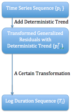
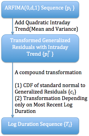
with Figure 1(b) showing more specific information for the model that we use for trade durations. The process that we used for choosing the components of the model is described in Section 4.1.

1. Underlying the process is a latent process $\{p_{i}\}_{i\geq 1}$ that captures the long-memory dependence. The latent process is modeled by a parametric time series model, e.g. autoregressive moving average (ARMA) or autoregressive fractionally integrated moving average (ARFIMA). If one needs to incorporate additional explanatory variables, one can augment the time series model with a regression component. Descriptions of ARFIMA models and the augmentation that we use for regression are is given in Appendix A.

2. A general time trend can be modeled so that the distribution of duration depends on both clock time and event time. Let $R(\cdot|time_{i-1})$ be a one-to-one, clock-time dependent, function of a real variable, where $time_{i-1}$ stands for the clock time at which event $i-1$ occurs. Applying the transformation produces the transformed process

   $$p^{T}_{i}=R(p_{i}|time_{i-1}).$$

3. Finally, the log-duration $T_{i}$ is a general past-dependent transformation of $p^{T}_{i}$, $T_{i}=H_{i}(p^{T}_{i})$.

Combining the above levels of the hierarchy, the distribution of $\{T_{i}\}_{i\geq 1}$ can be written in terms of the distribution of the latent process $\{p_{i}\}_{i\geq 1}$. Let $G_{i}(\cdot)$ denote the conditional distribution function of $p_{i}$ given the past. Then, the conditional distribution of $T_{i}$ given the past has CDF

$$F_{i}^{*}(t)=\Pr(T_{i}\leq t)=\Pr(p_{i}^{T}\leq H_{i}^{-1}(t))=G_{i}\left(R^{-1}[H_{i}^{-1}(t)|time_{i-1}]\right).$$ (3.1)

3.2 Estimation Method

Our proposed semiparametric estimation method proceeds by reversing the steps in the data generating process described above.

1. First, express the general transformation $H_{i}$ as $H_{i}(\cdot)=F_{i}^{-1}(\Phi(\cdot))$, where $F_{i}(\cdot)$ is a general cumulative distribution function (CDF) that depends on the past and $\Phi$ is the standard normal CDF. For trade durations, we find a nonparametric kernel estimator of $H_{i}$ as follows. Compute a conditional density estimator $\hat{f}_{i}(\cdot)$ for the log-durations $T_{i}$ given the previous log-duration $T_{i-1}$, and form the corresponding CDF, $\hat{F}_{i}(\cdot)=\hat{F}(\cdot|T_{i-1})$. Calculate the generalized residuals $c_{i}=\hat{F}_{i}(T_{i})$ and the transformed generalized residuals $\hat{p}^{T}_{i}=\Phi^{-1}(c_{i})$.

2. Model the clock-time dependent trend. For trade durations, we find that an intraday trend is both useful and meaningful. The specific form we use is

   $$R(p_{i}|time_{i-1})=p_{i}\tau_{\rm sd}(time_{i-1})+\tau_{\rm mean}(time_{i-1}),$$

   where $\tau_{\rm mean}$ and $\tau_{\rm sd}$ are respectively functions of clock time that model changes in the mean and standard deviation of $\{\hat{p}^{T}_{i}\}_{i\geq 1}$. Estimate the trends as $\hat{\tau}_{\rm mean}(time_{i-1})$ and $\hat{\tau}_{\rm sd}(time_{i-1})$, and then calculate the detrended sequence

   $$\hat{p}_{i}=\hat{R}^{-1}[\hat{p}^{T}_{i}|time_{i-1}]=\frac{\hat{p}^{T}_{i}-\hat{\tau}_{\rm mean}(time_{i-1})}{\hat{\tau}_{\rm sd}(time_{i-1})}.$$

   Specifically, we let both $\tau_{\rm mean}$ and $\tau^{2}_{\rm sd}$ be quadratic functions of clock time as described in more detail below.

3. Fit a parametric time series model to the detrended transformed generalized residuals: $TSmodel(\hat{p}_{i}|\{\hat{p}_{j}\}_{j=1}^{i-1})$. The fitted time series model will predict that each $\hat{p}_{i}$ given the past has a normal distribution with mean $\hat{\mu}_{i}$ and standard deviation $\hat{\sigma}_{i}$. If additional explanatory variables are needed, an appropriate modification is done at this step. Section A gives more details.

After the fit, transform back to the log-duration scale. The fitted value corresponding to the $i$th log-duration is

$$\hat{T}_{i}=\hat{F}_{i}^{-1}\left[\Phi\left(\frac{\hat{p}_{i}-\hat{\mu}_{i}}{\hat{\sigma}_{i}}\right)\right].$$

In step 1, $\hat{F}_{i}$ can be any past-dependent CDF. For trade durations, we try to capture a general form of the most important dependence, specifically the dependence on the previous log-duration, $T_{i-1}$. So, we use a nonparametric conditional density estimator for the density of $T_{i}$ given $T_{i-1}$, and convert the density into its corresponding CDF. If $\hat{F}_{i}$ were indeed the conditional CDF of $T_{i}$ given the past, then the generalized residuals $\{c_{i}\}_{i\geq 1}$ would be independent uniform random variables on the interval $(0,1)$, and $\hat{p}^{T}_{i}=\Phi^{-1}(c_{i})$ would be independent standard normal random variables. Of course, empirical evidence with trade durations suggests that the distribution of $\{\hat{p}^{T}_{i}\}_{i\geq 1}$ is much more complicated, having both time-varying mean and time-varying standard deviation, not to mention long memory.

In step 2, we detrend the $\hat{p}^{T}_{i}$. Both the mean and variance appear to be large in the middle of the day and smaller at the start and end of the day. So, we fit a quadratic trend for each:

$$\tau_{\rm mean}(t)=at^{2}+bt+c,\quad\tau^{2}_{\rm sd}(t)=dt^{2}+et+f.$$

Our model says that the

$$p_{i}=\frac{p_{i}^{T}-\tau_{\rm mean}(time_{i-1})}{\tau_{\rm sd}(time_{i-1})},$$

given the past, are a normally distributed process with time-series structure. We fit the trend parameters $\eta=(a,b,c,d,e,f)$ using quasi-maximum likelihood. The log-quasi-likelihood function that we use is

$$-\sum_{i=2}^{n}\left[\log\tau_{\rm sd}(time_{i-1})+\frac{[\hat{p}_{i}^{T}-\tau_{\rm mean}(time_{i-1})]^{2}}{2\tau_{\rm sd}(time_{i-1})^{2}}\right],$$ (3.2)

where $n$ is the number of durations in the day. The function in (3.2) would be the likelihood function if the $\hat{p}_{i}$ were independent rather than following a time-series model.

In step 3, we fit an appropriate time series model to the $\{\hat{p}_{i}\}_{i\geq 1}$ sequence assuming that the noise terms are normally distributed. With trade duration data, we fit an ARFIMA model with orders chosen by BIC. Each time series model then says that the distribution of $p_{i}$ is the normal distribution with a fitted mean $\hat{\mu}_{i}$ and fitted variance $\hat{\sigma}_{i}^{2}$ determined by the specific model.

Instead of maximizing the quasi-log-likelihood (3.2), we could attempt to find the joint MLE of $\eta$ and the parameters of the ARFIMA model. The log-likelihood for both sets of parameters is not (3.2), but rather

$$-\sum_{i=2}^{n}\left[\log[\tau_{\rm sd}(time_{i-1})\sigma_{i}]+\frac{[\hat{p}_{i}^{T}-\tau_{\rm mean}(time_{i-1})-\tau_{sd}(time_{i-1})\mu_{i}]^{2}}{2\tau_{\rm sd}(time_{i-1})^{2}\sigma_{i}^{2}}\right],$$ (3.3)

where $\mu_{i}$ and $\sigma_{i}$ are functions of the ARFIMA parameters that specify the mean and standard deviation of $p_{i}$ given the past. Note that (3.2) is the special case of (3.3) when $\mu_{i}=0$ and $\sigma_{i}=1$. Starting with $\mu_{i}=0$ and $\sigma_{i}=1$, steps 2 and 3 should be iteratively repeated, using (3.3) in step 2instead of (3.2), until the parameter estimates converge. Specifically, after the first round of steps 2 and 3, set $\mu_{i}$ and $\sigma_{i}$ respectively to the estimated mean and standard deviation of $p_{i}$ given the past as fit by the ARFIMA model in step 3. For later iterations, use the estimated $\mu_{i}$ and $\hat{\sigma}_{i}$ to refit the trend parameters by maximizing the log-likelihood in equation 3.3. With the new estimated trend parameters, refit the ARFIMA parameters and alternated until the estimated parameters converge. We compared this procedure to the quasi-likelihood maximization described above and found that the ARFIMA parameter estimates change negligibly (usually less than 1%). The trend parameters sometimes change as much as 15%, but the changes do not translate into noticeable changes in predictions. (We give more evidence of this last claim in Section 3.3.) The empirical results that we report in Section 4 use the quasi-likelihood maximization.

3.3 Prediction

When we wish to predict log-durations on a new day (which we will call test data), we start with the fitted model based on the previous day’s data (which we will call training data). We carry forward the conditional CDF $\hat{F}(\cdot|T_{i-1})$ and coefficients from the ARFIMA process that were estimated from the training data. For the the intraday trend, we assume that a new coefficient vector $\eta=(a,b,c,d,e,f)$ is needed each day. We start by using the estimated $\hat{\eta}=(a_{0},b_{0},c_{0},d_{0},e_{0},f_{0})$ from the training data. In order to perform updates to $\hat{\eta}$ in real time as events occur, a fast update is needed for $\hat{\eta}$. We propose the following penalized least squares estimation (LSE) method. Whenever a new pair of $(time_{j-1},p^{T}_{j})$ arrives from the test data, we update our estimated $\hat{\eta}$ as follows. Choose $(\hat{a},\hat{b},\hat{c})$ to minimize

$$\sum_{i=1}^{j}(p^{T}_{i}-a\times time_{i-1}^{2}-b\times time_{i-1}-c)^{2}+\lambda(a-a_{0})^{2}+\lambda(b-b_{0})^{2}+\lambda(c-c_{0})^{2},$$

and set

$$\hat{\tau}_{\rm mean}(time_{i-1})=\hat{a}\times time_{i-1}^{2}+\hat{b}\times time_{i-1}+\hat{c}.$$ (3.4)

Then choose $(\hat{d},\hat{e},\hat{f})$ to minimize

$$\sum_{i=1}^{j}[(p^{T}_{i}-\hat{\tau}_{\rm mean}(time_{i-1}))^{2}-d\times time_{i-1}^{2}-e\times time_{i-1}-f]^{2}+\lambda(d-d_{0})^{2}+\lambda(e-e_{0})^{2}+\lambda(f-f_{0})^{2},$$

and set

$$\hat{\tau}_{\rm sd}(time_{i-1})=\sqrt{\hat{d}\times time_{i-1}^{2}+\hat{e}\times time_{i-1}+\hat{f}.}$$ (3.5)

Empirical results depend little on the value of $\lambda$ for $\lambda$ in a large interval. We use $\lambda=10$ in our calculations.

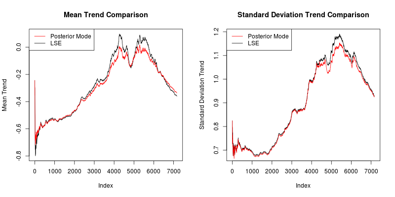
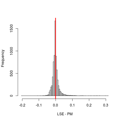
A more time-consuming, but perhaps more principled, method of updating the trend parameters would be to compute the posterior mode (PM) after each trade event. We could use the negatives of the penalizations in the LSE method log-priors and maximize the sum of those log-priors and the log-likelihood (3.3). The quality of the LSE approximation, compared to PM is illustrated in Figures 2 and 3. We see that the two update methods produce intraday trends that are very similar with predictions of comparable quality. Because LSE works many times faster than PM, we use LSE for prediction in the remainder of the paper.

Figure 2: Estimated intraday trends in both mean and standard deviation for one stock on one day. The black line gives the estimates based on LSE, and the red line gives the estimates based on PM.

Figure 3: Histogram of differences of individual prediction log-likelihoods (one for each predicted duration) between LSE and PM for JPM on one day. The mean and median are both close to 0, and the average of the individual prediction log-likelihoods is $-2.15$, so the percentage differences are also small. The other stocks and days have similar patterns.

In Section 4, we evaluate our model fit and compare it to the fits of other models. We fit all models using training data and then base the evaluations and comparisons on test data. We use the prediction log-likelihood and goodness-of-fit tests based on generalized residuals.

3.4 Predictive Distribution and Log-Likelihood

In this section, we show how to use estimates from the training data along with the continuously updated intraday trend described above to compute the predictive distribution of test data.

The fitted conditional CDF of the next $T_{i}$ in the test data given the past can be constructed using (3.1). The time series model says that our estimate of the conditional CDF $G_{i}$ is $\hat{G}_{i}(u)=\Phi([u-\hat{\mu}_{i}]/\hat{\sigma}_{i})$, where $\hat{\mu}_{i}$ and $\hat{\sigma}_{i}$ are based on the estimated ARFIMA parameters from the training data along with the past durations in the test data. Our estimate of $H_{i}$ from the training data is $\hat{H}_{i}=\hat{F}_{i}^{-1}(\Phi)$, so the estimated conditional CDF of $T_{i}$ is

$$\hat{F}_{i}^{*}(t)=\Phi\left(\frac{1}{\hat{\sigma}_{i}}\left[\frac{\Phi^{-1}(\hat{F}_{i}(t))-\hat{\tau}_{\rm mean}(time_{i-1})}{\hat{\tau}_{\rm sd}(time_{i-1})}-\hat{\mu}_{i}\right]\right),$$ (3.6)

where $\hat{\tau}_{\rm mean}$ and $\hat{\tau}_{\rm sd}$ come from (3.4) and (3.5) respectively, and are recomputed each time that a new event occurs.

In order to compute the prediction log-likelihood of the test data, we need the density corresponding to the CDF in (3.6). This is obtained by standard calculus operations as

$$\hat{f}_{i}^{*}(t)=\frac{1}{\hat{\tau}_{\rm sd}(time_{i-1})}\phi_{\hat{\mu}_{i},\hat{\sigma}_{i}}\left(\frac{\Phi^{-1}(\hat{F}_{i}(t))-\hat{\tau}_{\rm mean}(time_{i-1})}{\hat{\tau}_{\rm sd}(time_{i-1})}\right)\times\frac{\hat{f}_{i}(t)}{\phi_{0,1}(\Phi^{-1}(\hat{F}_{i}(t)))},$$ (3.7)

where, $\phi_{m,s}(\cdot)$ denotes the density of the normal distribution with mean $m$ and standard deviation $s$, and $\hat{f}_{i}$ is the density that corresponds to $\hat{F}_{i}$. The predictionlog-likelihood for the test data $\{T_{i}\}_{i=1}^{n}$ is $\sum_{i=1}^{n}\log(\hat{f}_{i}^{*}(T_{i}))$.

The form (3.7) has a convenient interpretation for comparing our model to some submodels. For example, if we ignore the intraday trend, then we just set $\hat{\tau}_{\rm mean}(\cdot)\equiv 0$ and $\hat{\tau}_{\rm sd}(\cdot)\equiv 1$. If we wish to ignore the ARFIMA modeling, we just set $\hat{\mu}_{i}=0$ and $\hat{\sigma}_{i}=1$.

The final generalized residual corresponding to $T_{i}$ from the test data is computed by substituting $T_{i}$ for $t$ in (3.6):

$$c^{*}_{i}=\hat{F}_{i}^{*}(T_{i})=\Phi\left(\frac{1}{\hat{\sigma}_{i}}\left[\frac{\Phi^{-1}(\hat{F}_{i}(T_{i}))-\hat{\tau}_{\rm mean}(time_{i-1})}{\hat{\tau}_{\rm sd}(time_{i-1})}-\hat{\mu}_{i}\right]\right),$$ (3.8)

If the model fits well, then the $c^{*}_{i}$ should look like a sample of independent uniform random variables on the interval $(0,1)$. We will present goodness-of-fit tests results based on $\{c^{*}_{i}\}_{i=1}^{n}$ in Section 4.

3.5 Additional Explanatory Variables

In a marked point process, marks are observed along with the target events. These marks, or additional explanatory variables, may have an impact on the distribution of log-duration. In the ACD model and its variants, the marks’ information is incorporated in the autoregressive formula (2.2). Analogously, in our model, it is natural to incorporate the additional variables’ effects in the parametric time-series model (step 3).

A straightforward way to incorporate additional variables into an ARFIMA model is to extend the ARMA model with regression R.H.Shumway and D.S.Stoffer (2011). We call the extension ARFIMA with regression. Various methods for estimating ARFIMA models have been reviewed in Chan and Palma (2006). In the trade duration example in Section 4, we use ARFIMA with regression in order to incorporate an additional explanatory variable into our model.

4 Experimental Results

In this section, the HSDM framework is applied to the trade flows from the limit order books of four stocks (IBM, JC Penny, JP Morgan, and Exxon Mobil) on the New York Stock Exchange (NYSE) for selected dates between 6 July 2010 and 29 July 2010, 18 consecutive trading days. In Section 4.1, the first eight days are used to build the model and discover patterns. In Section 4.3, we use the remaining days to validate the model and to make comparisons between HSDM and benchmark models. Each day is used as training data to estimate parameters and the following day is used as test data for prediction and goodness-of-fit tests. This pattern of training data followed by test data is used during both model building and validation.

Since the focus of this paper is on the dynamics of trade flow, the limit order book data are preprocessed, and a list of triples $(time_{i},T_{i},BPI_{i})$ is produced, where $time_{i}$ is the clock time, $T_{i}$ is log-duration, and $BPI_{i}$ (book pressure imbalance) is our additional explanatory variable. Table 1 gives a sample of three consecutive such triples.

Table 1: A sample of trade flow data. Clock time is in milliseconds since midnight, and log-duration is in log-milliseconds since previous trade.

clock time	log-duration	book pressure imbalance
43026177	3.91	-0.588
43026179	6.82	-0.134
43026180	6.10	-1.946

We observe such a triple whenever a trade occurs. Book pressure imbalance is defined as the logarithm of the ratio of the number of sell-side shares at the ask price to number of buy-side shares at the bid price. In general, it measures the imbalance of demand between the buy and sell sides of the market. BPI varies from time to time and actually changes much more frequently than trades occur. In this paper, we keep track of the book pressure imbalance only when a trade happens. Moreover, since the focus in this article is the duration between trades, it is the degree of imbalance rather than the direction of imbalance that matters. Thus, we use the absolute value of book pressure imbalance, $|BPI|$, as our additional explanatory variable.

In Section 4.1, we present empirical evidence that motivates each of the stages in the hierarchy of the HSDM framework. Section 4.2 describes the benchmark models to which we compare HSDM in Section 4.3.

4.1 Model Building

Here we show why we chose the particular stages in the hierarchy of the HSDM model of Section 3. The choices are based on a period of model building data ranging from 6 July 2010 to 16 July 2010. It is widely accepted that duration processes in market microstructure data are self-exciting (especially intertrade durations). Figure 4

Figure 4: Current log-duration (vertical axis) vs. previous log-duration (horizontal axis) for one stock on one day. Two key features are noted by the circled regions. The solid circles indicate the self-exciting nature by showing the clustering of pairs with both durations being short and with both durations being long. The dashed circles indicate the bimodal nature by showing secondary modes at both long and short durations regardless of the length of the other duration.

shows a scatter plot of the pairs of consecutive log-durations for one stock on one day. The plot shows that (i) long durations tend to be followed by long durations, while short durations tend to be followed by short duration (the self-exciting property) and (ii) the marginal distribution of log-duration and the conditional distribution of log-duration given the previous log-duration are bimodal. Since we expect the most recent durations to carry the most information, step 1 of the estimation procedure employs nonparametric kernel conditional density estimation as described by Hall, Racine and Li (2004) Hall, Racine and Li (2004), conditioning on the previous log-duration $T_{i-1}$. A technical issue arises due to the discreteness of durations, as they are measured to the nearest millisecond. We explain this issue in more detail in Appendix B along with how we deal with it. In particular, we explain why it makes sense to base the estimation on the logarithms of the durations. The estimated conditional CDF of $T_{i}$ given $T_{i-1}$ is denoted by $\hat{F}_{i}(\cdot)$. Figure 5

Figure 5: Conditional density of $T_{i}$ given $T_{i-1}$ for 12 different values of $T_{i-1}\in\{1,\ldots,12\}$. These range from $2.7\times 10^{-3}$ seconds to 2.7 minutes.

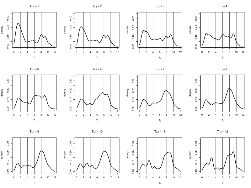
shows the conditional densities that were estimated conditional on different values of the previous log-duration $T_{i-1}$ for one day of one stock. The conditional densities capture the self-exciting feature of trades. Note how the conditional density is highest near zero when the previous duration is short, but when the previous duration is long, the density is highest at larger values. No matter what the previous duration $T_{i-1}$ is, the distribution of the current duration $T_{i}$ has two local modes. And as the previous duration increases, both the height and the location of the second mode increase. The bimodal characteristic partly explains why parametric conditional duration models with a unimodal residual distribution cannot capture the dynamics of trade flow very well. Nonparametric conditional density estimation in step 1 captures not only some short memory information but also the bimodal nature of the conditional distribution.

In step 2 of the estimation, we introduce intraday trends for both the mean and variance of the $\{p_{i}^{T}\}_{i\geq 1}$ sequence. Figure 6

Figure 6: Fitted intraday trends on eight different days (one color for each day) for both the mean and variance of $p_{i}^{T}$ for a single stock (JPM). The trends were fitted as moving average trends with window length equal 2000 trades fit to the $\hat{p}_{i}^{T}$.

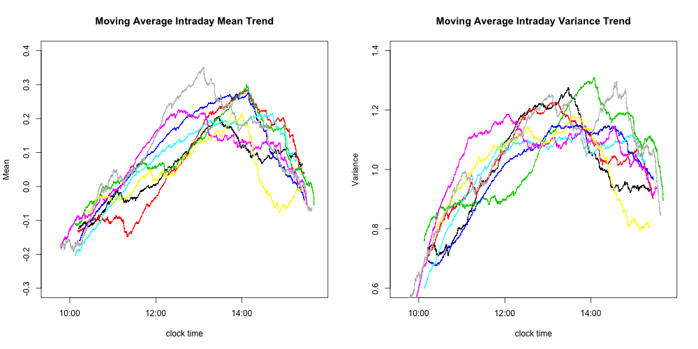
shows empirical evidence for those trends for eight different days and one stock. The mean trends in Figure 6 are computed as moving averages $m_{i}$ of the $\hat{p}^{T}_{i}$ sequences throughout each day. The trends for variance were computed as moving averages of $(\hat{p}^{T}_{i}-m_{i})^{2}$ throughout the day. The shapes suggest that an intraday trend is present in the data and that a quadratic shape might provide a good fit. The mean and the variance of $p_{i}^{T}$ have similar intraday patterns, but they change slightly from day to day. This apparent change motivates our online estimation of the parameters described in Section 3.3.

After detrending the $\hat{p}_{i}^{T}$ in step 2, we compute their autocorrelation function and partial autocorrelation function, which appear in Figure 7 for a typical trading day of JPM. These plots are typical of the patterns that we see across all of the four stocks and all days.

Figure 7: Sample ACF and PACF of transformed generalized residuals after detrending. The lag-zero autocorrelation of 1 is truncated in the ACF plot.

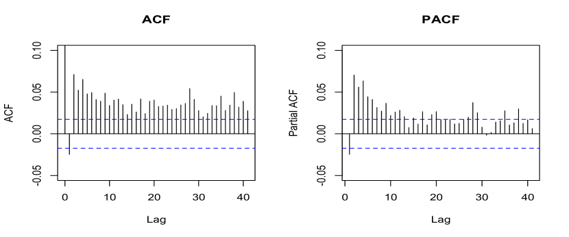
The patterns in these plots suggest the presence of long memory. The negative lag-one autocorrelation suggests that the conditional density estimation may be overfitting the lag-one dependence.

In step 3 of the estimation, we begin with a long-memory time series model having no exogenous variables. Appendix A provides some detail about both the time series model that we use (ARFIMA) and how we incorporate regression into that model. The particular model that we choose is ARFIMA(0,$d$,1), which has the form

$$(1-B)^{d}P_{i}=(1-\theta B)Z_{i},\ \ where\ \ Z_{i}\sim N(0,\sigma^{2}).$$ (4.1)

With our data sets, the differencing parameter $d$ is typically estimated to be around 0.1 (with standard error around $0.01$), suggesting significant long memory. We chose this from the family of ARFIMA($p,d,q$) models by minimizing the BIC score among the potential choices of $p\in\{0,1,2,3\}$ and $q\in\{0,1,2,3\}$.

4.2 The Benchmark Models

In this section, we implement four common members of the ACD family of models as benchmarks. These include exponential ACD, semiparametric ACD, exponential FIACD, and semiparametric FIACD. For each of these models, intraday patterns are estimated directly from the durations by fitting a cubic spline with knots at each full hour of clock-time. After fitting the spline, the $i$th duration is divided by the fitted spline value at $time_{i-1}$. The resulting ratios are used as the input data for the ACD model and its variants as Jaisk did in Jasiak (1999). For predicting test data, we use the estimated intraday pattern based on the previous day’s (training) data. All of the benchmark models start with the formula

$$X_{i}=\Psi_{i}\epsilon_{i},$$

where $X_{i}$ is a duration (divided by the intraday trend), $\Psi_{i}$ is the conditional mean of $X_{i}$, and $\epsilon_{i}$ are IID from a long-tailed distribution with mean 1. The exponential ACD and exponential FIACD, assume that $\epsilon_{i}$ has the standard exponential distribution while the semiparametric versions allow $\epsilon_{i}$ to have a general density $f(\cdot)$ that is fit by kernel density estimation. For the ACD and exponential ACD models, the conditional mean of $X_{i}$ evolves as

$$\Psi_{i}=\omega+\alpha X_{i-1}+\beta\Psi_{i-1}.$$

For the fractionally integrated versions, the conditional mean evolves as

$$(1-\beta)\Psi_{i}=w+[1-\beta-(1-\alpha-\beta)(1-B)^{d}]X_{i-1}.$$

After fitting these models we compare them all to HSDM in terms of prediction log-likelihood and various model diagnostics as described in Section 4.3.

4.3 Model Comparisons

In this section, we compare the five models based on prediction log-likelihood and a number of diagnostic tests using the validation data from 19 July 2010 through 29 July 2010. Diebold, Gunther and Tay (1998) Diebold, Gunther and Tay (1998) (henceforth DGT) proposed a method of evaluating prediction models based on the probability integral transform. If the predictive distribution of the $i$th observation $X_{i}$ given the past has the CDF $F_{i}(\cdot)$, then the sequence of values $\{F_{i}(X_{i})\}_{i\geq 1}$ forms an IID sample of uniform random variables on the interval (0,1). Of course, we don’t know $F_{i}$, but each model provides a fitted $\hat{F}_{i}$ for each $i$. We can then see to what extent the sequence of final generalized residuals, $\{\hat{F}_{i}(X_{i})\}_{i\geq 1}$, looks like a sample of IID uniform random variables on the interval (0,1). The empirical distribution of the sequence should look like a uniform distribution, and the sequence should not exhibit any autocorrelation.

For the HSDM model, the final generalized residuals, $c_{i}^{*}$ come from (3.8). Each of the other models has a corresponding final generalized residual to be tested, i.e. $c_{i}^{*}=\hat{F}(X_{i}/\hat{\Psi}_{i})$, where $\hat{F}(\cdot)$ is the estimated CDF of $\epsilon$ for each model. In the exponential ACD and exponential FIACD models, $\hat{F}(\cdot)$ is the CDF of the exponential distribution with mean 1, while in the semiparametric ACD and semiparametric FIACD, $\hat{F}(\cdot)$ is an estimate based on kernel density estimation using the fitted $\epsilon_{i}$ values as suggested by Jasiak (1999). In Appendix B.1 we give more detail on the kernel density estimation. In particular, we explain why it makes sense to base the estimation on the $\log(\epsilon_{i})$ values.

Bauwens, Giot, Grammig and Veredas (2000) BAUWENS et al. (2000) compared some of the most popular conditional duration models, including ACD, log ACD, threshold ACD, SCD and SVD, by means of the DGT method. Although they found that these models generally work well on the price duration process and the volume duration process, none of them work on the trade duration process.

There is one important distinction between the diagnostics that we compute and those computed in most other papers on self-exciting point process models. As in other papers, we first fit models to training data. The difference is that we compute the final generalized residuals by using the fitted models to predict test data. Most papers compute their diagnostics from the final generalized residuals obtained by predicting the same training data that were used to fit the models. There are two main reasons for using test data to perform the diagnostics rather than using training data. First, it is well-known that virtually all statistical models fit better to the data from which they were estimated than to new data that were not used for their estimation. It is good statistical practice to evaluate the fit of every model on test data, if such data are available. Second, we are comparing a number of models that are semiparametric along with some that do not form a nested sequence. Traditional likelihood-ratio tests are useful for comparing nested parametric models in order to see whether the additional parameters provide significant improvement or merely overfit. With semiparametric models, the theory of likelihood-ratio tests is still being developed. In order to minimize the chance of overfitting with semiparametric models, it is good practice to evaluate them with test data that were not used in the fitting. (This procedure is good practice even with parametric models.) If a model overfits the training data, it will make noisy predictions with test data. In comparing two or more models, comparing their predictions based on test data is the safest way to avoid choosing a model that was overfit.

4.3.1 Prediction Log-Likelihood

In this section, we compare the five models based on prediction log-likelihood for test data. This is essentially a comparison based on how high is each model’s predictive density at the observed test data. The larger the prediction log-likelihood, the better the prediction is. Figure 8

Figure 8: Comparison between HSDM model and benchmark models in terms of negative prediction log-likelihood. Smaller is better.

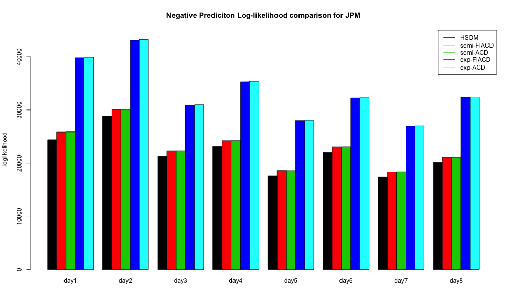
shows the negative prediction log-likelihood for JPM on the eight consecutive test days in the validation data for all five models. The HSDM model (black bars) is consistently better than all of the benchmark models. And within the four benchmark models, semi-parametric models are better than exponential models. ACD models and FIACD models exhibit similar performance. The other three stocks (IBM, XOM, JCP) have similar patterns. the HSDM and benchmark model perform on each individual observation is of great interest. Figure 9

Figure 9: Histogram of differences between individual log-likelihoods, HSDM minus the best benchmark model (semiparametric-FIACD) on a typical day of JPM. The red vertical line is the mean ($\approx 0.122$). The median is 0.124, and the percentage of differences that are positive is 62.4%.

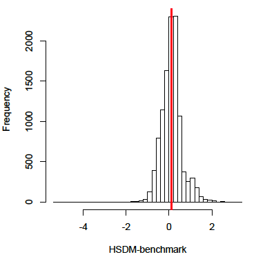
compares the performance of HSDM and the best benchmark model, semiparametric FIACD, on a typical day of JPM. The plot displays the histogram of differences of individual prediction log-likelihood between HSDM and semiparametric FIACD. The positive part of the histogram corresponds to those observations on which HSDM has a better prediction than semiparametric FIACD, while the negative part corresponds to observations on which HSDM performs worse than semiparametric FIACD. The mean of the difference is around 0.122 (denoted by the red vertical line), the median is around 0.124, and the percentage of positive differences is 62.4%. All of the other days and stocks have similar patterns.

4.3.2 Uniform Test

In this section, we compare each set of final generalized residuals to the uniform distribution on the interval (0,1) by means of the Kolmogorov-Smirnov (KS) test. The left subfigure in Figure 10

Figure 10: Q-Q plots of $p$-values from KS test and Ljung-Box test on HSDM and benchmark models.

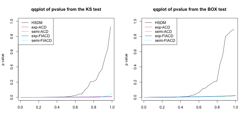
shows the Q-Q plot of 32 $p$-values from KS tests for each of the five models (8 test days for each of 4 stocks). If the final generalized residuals were really sampled from their predictive distributions, then the $p$-values should be uniformly distributed on the interval $(0,1)$ and the the Q-Q plot should be around the 45-degree line. If the final generalized residuals come from different distributions, the $p$-values should be stochastically smaller than uniform on $(0,1)$.

Since each model estimates a predicitive distribution from the observed data (including training data), we cannot expect the $p$-values to be uniformly distributed. When the estimated distributions come from a finite-dimensional parametric family, there are modifications available to the KS test so that the $p$-values have uniform distribution asymptotically. When the predictive distributions are estimated nonparametrically or semiparameterically, the appropriate modifications have not yet been determined. Nevertheless, the KS test statistics (or equivalently their $p$-values) still give a means for comparing models based on how close to uniform the final generalized residuals appear to be. From the comparison in Figure 10, it is clear the benchmark models have (empirically) stochastically smaller $p$-values than HSDM. The HSDM $p$-values are still stochastically smaller than the uniform distribution, but they are much larger than those for the benchmark models.

The reason that the $p$-values from the exponential models are all so small is that the data come from a distribution with a much fatter tail than that of the exponential distribution. As a matter of fact, no popular parametric model can perform satisfactorily because the empirical log-duration has a bimodal shape. The semiparametric models perform relatively better but still have very small $p$-values.

4.3.3 Autocorrelation Test

In this section, we assess the degree of autocorrelation in the final generalized residuals. We used the Ljung-Box test with lags of 5, 10, and 15. The test is conducted on each of the 32 pairs of stock/test day for each model. The right subfigure in Figure 10 shows Q-Q plots of 32 $p$-values for the Ljung-Box test with lag 10 for all five models. The results of lags 5 and 15 are similar. If there were no autocorrelations, the $p$-vaules should be uniformly distributed on the interval $(0,1)$. If there are autocorrelations, the $p$-values should be stochastically smaller. The four benchmark models have $p$-values that are stochastically much smaller than those of HSDM. of the Box test. Although the qqplot of HSDM shows that the p values are not from a standard uniform distribution, it is significantly better than all of the four benchmark models, which almost have all 0 $p$-values. The reason that the $p-$values are so low for the benchmark models is that they don’t capture the information of the most recent duration very well. The HSDM model captures this information non parametrically, which helps eliminate lag-one autocorrelation from the final generalized residuals. In summary, the HSDM model captures the time dependency significantly better than the benchmark models.

4.4 Additional Explanatory Variables

As mentioned earlier, the effects of exogenous variables can be incorporated in step 3 of the HSDM framework by extending the parametric time series model with regression. As an example, we took into account book pressure imbalance (BPI) (defined in Section 4) as additional explanatory variables. Other variables, such as spread and volume, may be considered similarly. Figure 11

Figure 11: Effects of BPI on detrended P. Detrended P vs absolute value of BPI on a typical day of JPM. A significant downward trend is noticeable.

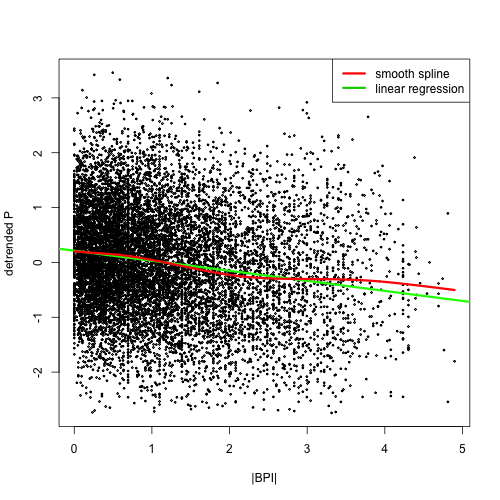
plots $\hat{p}_{i}$ (detrended $\hat{p}^{T}_{i}$) against $|{\rm BPI}_{i}|$ on a typical day of JPM. The red curve is a fitted smoothing spline, while the green line is the fitted linear regression. Apparently, as the absolute value of BPI increases, which means that there is more imbalance between buy side and sell side, $\hat{p}_{i}$ becomes smaller, leading to a shorter duration as expected. And the effect is close to a linear relationship. We choose how many lags of BPI to include in the regression by BIC. It turns out that the number of lags varies by stock. For example, the inclusion of two lags of BPI improves the prediction on JPM and XOM significantly, while there is no noticeable improvement with IBM and JCP. There is no reason that the same exogenous variables should be included in the models for all stocks, hence each stock will be modeled either with or without inclusion of BPI as we determine during the model building stage. Equation (4.2) is the ARFIMA with regression model for those stocks that use two lags of BPI.

$$(1-B)^{d}(P_{i}-b_{0}-b_{1}|BPI_{i-1}|-b_{2}|BPI_{i-2}|)=(1-\theta B)Z_{i},\ \ Z_{i}\sim N(0,\sigma^{2})$$ (4.2)

Figure 12

Figure 12: Increase in prediction log-likelihood by incorporation of $|BPI|$ for JPM as a fraction of the increase of HSDM (without BPI) over semiparametric-FIACD, i.e., equation (4.3).

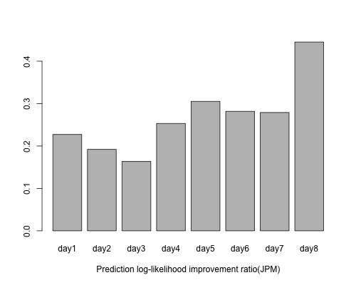
shows the increase in prediction log-likelihood from incorporating BPI as in 4.2 as a fraction of the amount by which HSDM (without $|BPI|$) improves over the best benchmark model (semiparametric-FIACD) for each of 8 days for JPM. That is, the plot shows

$$\frac{ll_{\rm HSDM\ with\ BPI}-ll_{\rm HSDM\ without\ BPI}}{ll_{\rm HSDM\ without\ BPI}-ll_{\rm semiparametric-FIACD}}.$$ (4.3)

The consistent large positive ratios across 8 validation days’ data indicate that the incorporation of BPI as in equation 4.2 further improves the model significantly on JPM.

The model constructed in this section is merely an illustration of how one might incorporate an exogenous variable into HSDM, hence, we did not include BPI in the benchmark models for comparison.

5 Discussion and Conclusion

We proposed a semiparametric framework for estimating the joint distribution of a marked point process. In particular, we applied our framework to trade duration processes. Using validation data that were not used to fit the models, the DGT evaluation methods (Diebold, Gunther and Tay, 1998 Diebold, Gunther and Tay (1998)), show that our model does consistently better than a number of benchmark models that are variants of the widely-used ACD model. The evaluation methods include Kolmogorov-Smirnov tests for uniformity of final generalized residuals and Ljung-Box tests for lack of autocorrelation. Bauwens, Giot, Grammig and Veredas (2000) BAUWENS et al. (2000) claimed that the parametric ACD model and all of its parametric variants fail to pass both the Kolmogorov-Smirnov test and the Ljung-Box test. This paper also shows that even semiparametric ACD models and their variants perform poorly in the sense of DGT evaluation methods, while HSDM shows a consistent improvement over the benchmark models. In addition, the HSDM model has a consistently better performance than the ACD model and its variants in the sense of prediction log-likelihood on validation data. Therefore, our framework has great potential for modeling the distributions of duration processes, especially the trade duration process.

The framework has two important features. First, it recognizes that both the shapes of distributions and the time dependency must be modeled. Nonparametric conditional density estimation captures the shapes of distributions along with the most recent time dependence. Parametric time series models capture the longer-term time dependency. Nonparametric estimation of the most recent time dependency gives the model greater flexibility. Second, our estimation procedure adaptively fits the intraday trend so as to capture changes that occur from day to day.

The two features described above help to explain why the HSDM procedure outperforms the existing ACD family on trade duration processes. Some of these features could be incorporated into ACD models and their fitting. Such incorporation will be the focus of future work. However, every model that is based on equation (2.1) will continue to suffer from some of the limitations mentioned in Section 2.3.

Appendix

Appendix A ARFIMA and ARFIMA With Regression Models

Equation (A.1) shows the formula for the general ARFIMA($p,d,q$) model for a response variable $Y$.

$$\left(1-\sum_{j=1}^{p}\phi_{j}B^{j}\right)(1-B)^{d}Y_{i}=\left(1+\sum_{j=1}^{q}\theta_{i}B^{j}\right)Z_{i},\ \ Z_{i}\sim N(0,\sigma^{2}),$$ (A.1)

where $(1-B)^{d}$ is defined by the generalized binomial series expansion as follows:

$$(1-B)^{d} = \sum_{k=0}^{\infty}\left(\begin{array}[]{c}d\\ k\end{array}\right)(-B)^{k}$$

$$= \sum_{k=0}\frac{\Pi_{a=0}^{k-1}(d-a)(-B)^{k}}{k!}$$

$$= 1-dB+\frac{d(d-1)}{2!}B^{2}-...,$$

where $B$ is the backshift operator. The R package fracdiff fracdiff (2012) can be used to fit ARFIMA models.

Suppose that we have $k$ auxiliary variables $U_{1},\ldots,U_{k}$ that we contemplate using to help predict $Y$. The ARFIMA with regression model replaces $Y_{i}$ in (A.1) with

$$Y_{i}-\alpha_{0}-\sum_{j=1}^{k}\alpha_{j}u_{i,j},$$

where $u_{i,j}$ is the value of $U_{j}$ that corresponds to $Y_{i}$, and $\alpha_{0},\ldots,\alpha_{k}$ are additional parameters to be estimated.

Appendix B Issues Related to Nonparametric Density Estimation

Throughout this section, $X_{i}$ and $T_{i}$ denote the original duration and log-duration respectively. The duration variable $X$ is measured in milliseconds and is hence discrete. It ranges from 1 millisecond up to more than 50000 milliseconds and exhibits an extremely long tail. We explain how we deal with the long tail in Section B.1, and we explain how we deal with the discreteness in Section B.2.

B.1 The Tail of the Distribution

Figure 13

Figure 13: Left panel: histogram of durations for one stock on one day. Right panel: histogram of log-durations on the same day.

shows histograms of durations for one stock on one day both in the original scale and in the log scale. The discreteness is merely an artifact of the measurement process, and we would want to model duration as a continuous variable. The logarithm transformation is employed before modeling, due to the fact that the long tail makes kernel conditional density estimation with a single bandwidth unreliable. For example, a bandwidth small enough to avoid merging everything in the first bar of the left panel in Figure 13 will be far too small for the upper tail of the distribution. Density estimation on log-durations is equivalent to using a variable bandwidth on the original scale. For the reasons given above, we do all kernel density estimation on the log scale for HSDM. Likewise in the semiparametric variations of ACD, the long tail of the residuals $\epsilon$ also calls for kernel density estimation (KDE) on the log scale. The two subfigures in Figure 14

(a)

(b)

Figure 14: (a) Histogram of semiparametric ACD residuals. (b) Histogram of semiparametric ACD residuals in log scale. Each plot has superimposed the density of the standard exponential distribution along with two densities estimated by KDE: one based on the original residuals, and the other based on log-residuals.

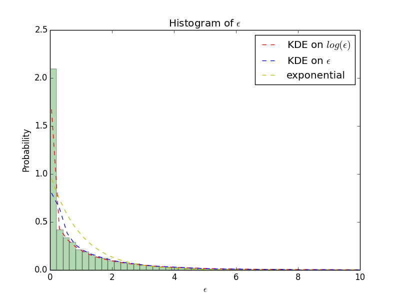
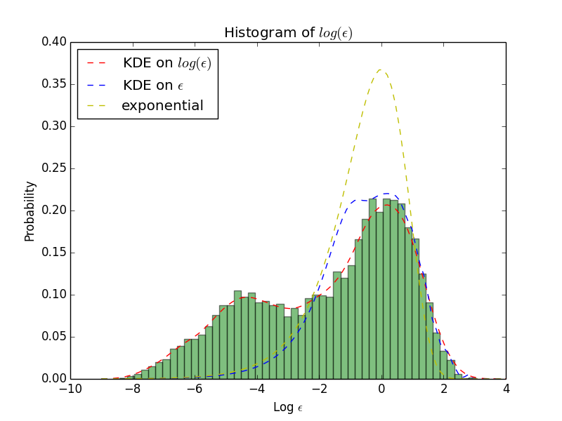
show the histograms of FIACD residuals $\epsilon$ in the original scale and the log scale. Superimposed on each histogram are three fitted densities in the corresponding scales. The three densities are those of the standard exponential distribution, a density estimated by KDE in the original scale, and one estimated by KDE in the log scale. It is obvious that KDE in the log scale captures the distribution of residuals more accurately. Therefore, kernel density estimation is applied to $log(\epsilon)$ in semiparametric variants of ACD.

B.2 Discreteness

Because the duration data are equally spaced (one-millisecond gaps), the logarithms have larger gaps at low values and smaller gaps at large values. Since the durations are denser at low values, automatic bandwidth selectors will tend to choose small bandwidths that put the most common log-durations into separate bins while undersmoothing the upper tail. This is counterproductive, and there is a simple method for obtaining more reasonable bandwidths. We can replace each discretely-recorded duration $X_{i}$ by $X_{i}-U_{i}$, where $U_{i}$ is an independently-generated noise value supported on an interval of length one millisecond. We choose $U_{i}$ to be uniform on the interval $(0,1)$. Let $Y_{i}=\log(1+X_{i}-U_{i})$. The reason for adding the 1 before taking the logarithm is that $X_{i}=1$ corresponds to $\log(X_{i}-U_{i})<0$. If we used these data, kernel density estimation would waste much of its effort estimating a density on $(-\infty,0)$, while the data have no information to distinguish these values. So, we use the sequence $\{Y_{i}\}_{i\geq 1}$ to construct a conditional kernel density estimate $g(\cdot|Y_{i-1})$, and then we convert this to an estimated conditional density $\hat{f}_{i}$ for $T_{i}=\log[\exp(Y_{i})-1]$ given $T_{i-1}=t_{i-1}$ by

$$\hat{f}_{i}(t)=g(\log[1+\exp(t)]|\log[1+\exp(t_{i-1})])\frac{\exp(t)}{1+\exp(t)},\mbox{\ for $t>0$,}$$

for use in step 1 of the HSDM estimation.

Next, we give some justification for subtracting uniform random variables before taking logarithms. Subtracting a uniform random variable from an integer-valued discrete random variable is motivated by the discrete version of the probability integral transform (PIT). The well-known continuous version of the PIT is the following.

Let $\{Z_{i}\}_{i\geq 1}$ be a sequence of random variables such that $Z_{1}$ has CDF $F_{1}$, and the conditional CDF of $Z_{i}$ given $Z_{1}=z_{1},\ldots,Z_{i-1}=z_{i-1}$ is $F_{i}(\cdot|z_{1},\ldots,z_{i-1})$ for $i>1$. Assume that $F_{i}$ is a continuous CDF for all $i$. Define $W_{1}=F_{1}(Z_{1})$ and $W_{i}=F_{i}(Z_{i}|Z_{1},\ldots,Z_{i-1})$ for $i>1$. Then $\{W_{i}\}_{i\geq 1}$ are IID random variables with the uniform distribution on the interval $(0,1)$.

The less well-known general version of the PIT is the following, of which Proposition LABEL:pro:pit is a corollary.

Lemma 1 (General PIT).

Let $\{X_{i}\}_{i\geq 1}$ be a sequence of random variables such that $X_{1}$ has CDF $F_{1}$, and the conditional CDF of $X_{i}$ given $X_{1}=x_{1},\ldots,X_{i-1}=x_{i-1}$ is $F_{i}(\cdot|x_{1},\ldots,x_{i-1})$ for $i>1$. Define $F^{\prime}_{1}(x)=\lim_{y\uparrow x}F_{1}(y)$, and for each $i>1$ and each vector $(x_{1},\ldots,x_{i-1},x)$ define $F^{\prime}_{i}(x|x_{1},\ldots,x_{i-1})=\lim_{y\uparrow x}F_{i}(y|x_{1},\ldots,x_{i-1})$. Also, define $J_{1}(x)=F_{1}(x)-F^{\prime}_{1}(x)$ and for $i>1$ define $J_{i}(x|x_{1},\ldots,x_{i-1})=F_{i}(x|x_{1},\ldots,x_{i-1})-F^{\prime}_{i}(x|x_{1},\ldots,x_{i-1})$. ($J_{i}$ measures the sizes of any jumps in the CDF $F_{i}$.) Let $\{V_{i}\}_{i\geq 1}$ be a sequence of IID uniform random variables on the interval $(0,1)$ that are independent of $\{X_{i}\}_{i\geq 1}$. Define $W_{1}=F_{1}(X_{1})-(1-V_{1})J_{1}(X_{1})$ and for $i>1$ define

$$W_{i}=F_{i}(X_{i}|X_{1},\ldots,X_{i-1})-(1-V_{i})J_{i}(X_{i}|X_{1},\ldots,X_{i-1}).$$ (B.1)

Then $\{W_{i}\}_{i\geq 1}$ are IID random variables with the uniform distribution on the interval $(0,1)$.

Proof. For each $i>1$ and each $0<p<1$, define

$$Q_{i}(p|x_{1},\ldots,x_{i-1})=\inf\{x:F_{i}(x|x_{1},\ldots,x_{i-1})\geq p\},$$

the generalization of the quantile function to general distributions, which is continuous from the left on $(0,1)$. For $0<p<1$, $W_{i}\leq p$ if and only if

$$\mbox{either\ }X_{i}<Q_{i}(p|X_{1},\ldots,X_{i-1}) \left(X_{i}=Q_{i}(p|X_{1},\ldots,X_{i-1})\phantom{\frac{p}{J}}\right.$$  or

$$\left.\mbox{\ and\ }V_{i}\leq\frac{p-F^{\prime}(Q_{i}(p|X_{1},\ldots,X_{i-1}))}{J_{i}(X_{i}|X_{1},\ldots,X_{i-1})}\right).$$

Hence,

$$\Pr(W_{i}\leq p|W_{1},\ldots,W_{i-1},X_{1},\ldots,X_{i-1})$$

$$= F^{\prime}(Q_{i}(p|X_{1},\ldots,X_{i-1}))$$

$$+J_{i}(p|X_{1},\ldots,X_{i-1})\frac{p-F^{\prime}_{i}(Q_{i}(p|X_{1},\ldots,X_{i-1}))}{J_{i}(X_{i}|X_{1},\ldots,X_{i-1})}$$

$$= p,$$

and $W_{i}$ has the uniform distribution on $(0,1)$ conditional on $W_{1},\ldots,W_{i-1},X_{1},\ldots,X_{i-1}$. It follows that $W_{i}$ is independent of $W_{1},\ldots,W_{i-1},X_{1},\ldots,X_{i-1}$ and hence is independent of $W_{1},\ldots,W_{i-1}$. The proof that $W_{1}$ has the uniform distribution is essentially the same as above without the conditioning. $\Box$

We now combine the two versions of the PIT to justify subtracting independent uniform random variables from integer-valued random variables.

Lemma 2.

Assume the same conditions and notation as in Lemma 1, and assume further that each $X_{i}$ is integer valued. Let $Z_{i}=X_{i}-V_{i}$ for each $i$. Let $G_{1}$ be the CDF of $Z_{1}$, and let $G_{i}$ be the conditional CDF of $Z_{i}$ given $Z_{1},\ldots,Z_{i-1}$ for $i>1$. Each $G_{i}$ is a continuous CDF. Also, $W_{1}=G_{1}(Z_{1})$ and $W_{i}=G_{i}(Z_{i}|Z_{1},\ldots,Z_{i-1})$ for $i>1$, where $W_{1}$ and $W_{i}$ are defined in Lemma 1.

Proof. For each $i$, $X_{i}=\lfloor Z_{i}\rfloor+1$ and $V_{i}=X_{i}-Z_{i}$, so that conditioning on the $Z_{i}$’s is equivalent to conditioning on the $X_{i}$’s and the $V_{i}$’s. It is straightforward to see that each $G_{i}$ is the linear interpolation of $F_{i}$ between consecutive integers. That is

$$G_{i}(z|z_{1},\ldots,z_{i-1})$$ (B.5)

$$= \left\{\begin{array}[]{ll}F_{i}(z|x_{1},\ldots,x_{i-1})&\mbox{if $z$ is an integer,}\\ F_{i}(\lfloor z\rfloor|x_{1},\ldots,x_{i-1})+(z-\lfloor z\rfloor)J_{i}(\lfloor z\rfloor+1|x_{1},\ldots,x_{i-1})&\mbox{otherwise.}\end{array}\right.$$

It follows that

$$G_{i}(Z_{i}|Z_{1},\ldots,Z_{i-1})$$

$$= F_{i}(X_{i}-1|X_{1},\ldots,X_{i-1})+(1-V_{i})[F_{i}(X_{i}|X_{1},\ldots,X_{i-1})$$

$$-F_{i}(X_{i}-1|X_{1},\ldots,X_{i-1})]$$

$$= F_{i}(X_{i}|X_{1},\ldots,X_{i-1})-(1-V_{i})J_{i}(X_{i}|X_{1},\ldots,X_{i-1})=W_{i}.$$

$\Box$

Lemma 2 tells us that we can compute generalized residuals two equivalent ways if we start with integer-valued random variables. One way is to use the general PIT in Lemma 1 directly on the integer-valued random variables. If the integer-valued random variables are the result of rounding up unobserved continuous random variables, we might prefer to smooth out the integers over the preceding interval and use the continuous PIT. Lemma 2 tells us that we get exactly the same sequence of generalized residuals either way, so long as we use the same sequence of uniform random variables for the smoothing as we use for Lemma 1.

There is one further connection between the smoothed and integer-valued random variables. They have the same prediction log-likelihood.

Lemma 3.

Assume the same conditions as in Lemma 2. Then for each integer $x$ and each $z\in(x-1,x)$,

$$J_{i}(x|x_{1},\ldots,x_{i-1}) = \Pr(X_{i}=x|X_{1}=x_{1},\ldots,X_{i-1}=x_{i-1})$$

$$= g_{i}(z|x_{1},\ldots,x_{n}),$$

where $g_{i}$ is the conditional density of $Z_{i}$ given $Z_{1}=z_{1},\ldots,Z_{i-1}=z_{i-1}$.

Proof. The proof is straightforward from (LABEL:eq:pit3), since $G_{i}$ is piecewise linear and the slope of $G_{i}$ on the open interval of length 1 to the left of each integer $x$ is $J_{i}(x|x_{1},\ldots,x_{i-1})$. $\Box$

Of course, all of the previous discussion relies on knowing all of the conditional CDFs of the integer-valued random variables. In our modeling of durations, we must estimate these distributions. Since we think of the durations as having continuous distributions in an ideal system, we choose the smoothing method. First, we smooth the integer-valued durations, then we estimate the conditional distributions. Our estimated distributions will not be piecewise linear as are the $G_{i}$ in Lemma 2. Since both the training data and test data are integer-valued, we convert our conditional distributions back to either discrete or smoothed distributions whichever makes the desired calculations simpler.

B.3 Random Effect of Smoothing

To better understand the extent to which smoothing the integer-valued durations affects our results, we ran experiments in which we repeated the smoothing using several independent sequences of uniform random variables (the $V_{i}$’s.) We found that the construction of $\hat{f}_{i}$ in step 1 and the fit of the ARFIMA model in step 3 produced indistinguishable results from one smoothing to the next. Also, the final generalized residuals behave the same with regard to the various diagnostics and the prediction log-likelihood from one smoothing to the next.

Figure 15

Figure 15: Histograms of ratio (B.6). One ratio is calculated for each of the 32 stock/date pairs. The Left subfigure is for HSDM, and the right subfigure is for semiparametric-FIACD.

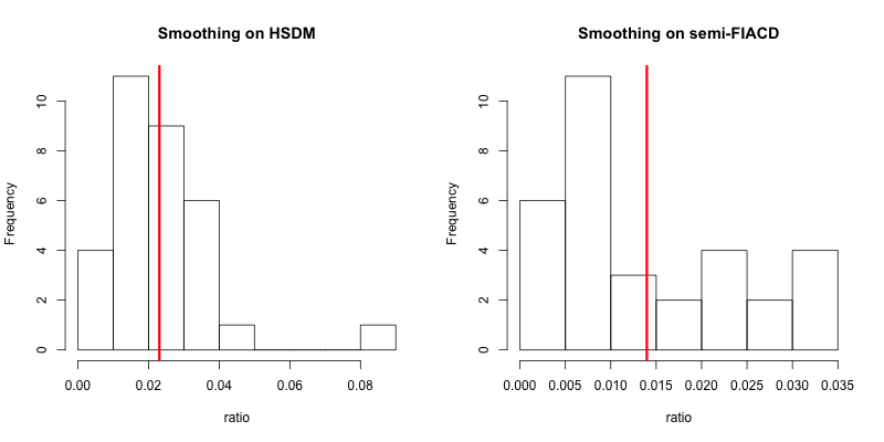
shows that the improvement of the HSDM model over the best benchmark model (semiparametric-FIACD) is robust in the sense of prediction log-likelihood under multiple smoothings of the integer-valued observations. We did three smoothings on each of 32 stock/day pairs. The left subfigure is the histogram of the range of the three different prediction log-likelihoods from different smoothings as a fraction of the amount by which the HSDM prediction log-likelihood exceeds that of the semiparametric-FIACD, i.e.

$${\rm ratio}=\frac{\max\{ll_{1},ll_{2},ll_{3}\}-\min\{ll_{1},ll_{2},ll_{3}\}}{ll_{\rm HSDM}-ll_{\rm semiparametric-FIACD}},$$ (B.6)

where $ll_{i}$ is the log-likelihood of HSDM under the $i$th different smoothing for $i=1,2,3$. The vertical red line is the average. In summary, the deviation caused by smoothing is only 2 percent of the improvement in prediction log-likelihood. Similarly, the right subfigure shows the distribution of ratio in (B.6) when smoothing is applied to the semiparametric-FIACD model. The effect of smoothing on the semiparametric-FIACD model is even smaller. Although the semiparametric-FIACD model does not require smoothing, doing the same smoothing as we do in the HSDM model gives a fairer comparison between the two models.

References

- Bauwens and Giot (2000) {barticle}[author] \bauthor\bsnmBauwens, \bfnmL.\binitsL. and \bauthor\bsnmGiot, \bfnmP.\binitsP. (\byear2000). \btitleThe logarithmic ACD model: An application to the Bid/Ask quote process of two NYSE stocks. \bjournalAnnales d Economie et de Statistique, 60:117 149. \endbibitem
- Bauwens and Hautsch (2006) {barticle}[author] \bauthor\bsnmBauwens, \bfnmLuc\binitsL. and \bauthor\bsnmHautsch, \bfnmNikolaus\binitsN. (\byear2006). \btitleMODELLING FINANCIAL HIGH FREQUENCY DATA USING POINT PROCESSES. \bjournalCore Discussion Paper. \endbibitem
- Bauwens and Veredas (2004) {barticle}[author] \bauthor\bsnmBauwens, \bfnmL.\binitsL. and \bauthor\bsnmVeredas, \bfnmD.\binitsD. (\byear2004). \btitleThe stochastic conditional duration model: A latent factor model for the analysis of financial durations. \bjournalJournal of Economet- rics, 119:381 412. \endbibitem
- BAUWENS et al. (2000) {barticle}[author] \bauthor\bsnmBAUWENS, \bfnmLuc\binitsL., \bauthor\bsnmGIOT, \bfnmPierre\binitsP., \bauthor\bsnmGRAMMIG, \bfnmJoachim\binitsJ. and \bauthor\bsnmVEREDAS, \bfnmDavid\binitsD. (\byear2000). \btitleA COMPARISON OF FINANCIAL DURATION MODELS VIA DENSITY FORECASTS. \bjournalCORE DISCUSSION PAPER 2000/60. \endbibitem
- C., Monfort and Trognon (1984) {barticle}[author] \bauthor\bsnmC., \bfnmGourieroux.\binitsG., \bauthor\bsnmMonfort, \bfnmA.\binitsA. and \bauthor\bsnmTrognon, \bfnmA.\binitsA. (\byear1984). \btitlePseudo-Maximum Likelihood Methods: Theory. \bjournalEconometrica. \endbibitem
- Chan and Palma (2006) {barticle}[author] \bauthor\bsnmChan, \bfnmNgai Hang\binitsN. H. and \bauthor\bsnmPalma, \bfnmWilfredo\binitsW. (\byear2006). \btitleEstimation of Long-memory Time Series Models: A Survey of Different Likelihood-Based Methods. \bjournalEconometric Analysis of Financial and Economic Time Series/Part B, Volumn 20, 89-121. \endbibitem
- Diebold, Gunther and Tay (1998) {barticle}[author] \bauthor\bsnmDiebold, \bfnmF. X.\binitsF. X., \bauthor\bsnmGunther, \bfnmT. A.\binitsT. A. and \bauthor\bsnmTay, \bfnmA. S.\binitsA. S. (\byear1998). \btitleEvaluating density forecasts, with applications to financial risk management. \bjournalInternational Economic Review, 39:863 883. \endbibitem
- Engle and Russell (1998) {barticle}[author] \bauthor\bsnmEngle, \bfnmR. F.\binitsR. F. and \bauthor\bsnmRussell, \bfnmJ. R.\binitsJ. R. (\byear1998). \btitleAutoregressive conditional duration: A new model for irregularly spaced transaction data. \bjournalEconometrica, 66:1127 1162. \endbibitem
- Ghysels, Gourieroux and Jasiak (2004) {barticle}[author] \bauthor\bsnmGhysels, \bfnmE.\binitsE., \bauthor\bsnmGourieroux, \bfnmC.\binitsC. and \bauthor\bsnmJasiak, \bfnmJ.\binitsJ. (\byear2004). \btitleStochastic volatility duration models. \bjournalJournal of Econometrics, 119:413 433. \endbibitem
- Hall, Racine and Li (2004) {barticle}[author] \bauthor\bsnmHall, \bfnmPeter\binitsP., \bauthor\bsnmRacine, \bfnmJeff\binitsJ. and \bauthor\bsnmLi, \bfnmQi\binitsQ. (\byear2004). \btitleCross-Validation and the Estimation of Conditional Probability Densities. \bjournalJournal of the American Statistical Association, Vol. 99, No. 468 (Dec., 2004), pp. 1015- 1026. \endbibitem
- Hasbrouck, Sofianos and Sosebee (1993) {barticle}[author] \bauthor\bsnmHasbrouck, \bfnmJ.\binitsJ., \bauthor\bsnmSofianos, \bfnmG.\binitsG. and \bauthor\bsnmSosebee, \bfnmD.\binitsD. (\byear1993). \btitleOrders, Trades, .Reports and Quotes and New York Stock Exchange. \bjournalWorking Paper, NYSE. \endbibitem
- Hawkes (1971) {barticle}[author] \bauthor\bsnmHawkes, \bfnmA. G.\binitsA. G. (\byear1971). \btitleSpectra of some self-exciting and mutually exciting point processes. \bjournalBiometrika, 58:83 90. \endbibitem
- Hujer, Vuletic and Kokot (2002) {barticle}[author] \bauthor\bsnmHujer, \bfnmReinhard\binitsR., \bauthor\bsnmVuletic, \bfnmSandra\binitsS. and \bauthor\bsnmKokot, \bfnmStefan\binitsS. (\byear2002). \btitleThe Markov Switching ACD model. \endbibitem
- Jasiak (1999) {barticle}[author] \bauthor\bsnmJasiak, \bfnmJoanna\binitsJ. (\byear1999). \btitlePersistence in Intertrade Durations. \endbibitem
- Pacurar (2006) {barticle}[author] \bauthor\bsnmPacurar, \bfnmMaria\binitsM. (\byear2006). \btitleAutoregressive Conditional Duration (ACD) Models in Finance: A survey of the Theoretical and Empirical Literature. \bjournalISSN: 1707-410X. \endbibitem
- R.H.Shumway and D.S.Stoffer (2011) {barticle}[author] \bauthor\bsnmShumway, \bfnmR. H.\binitsR. H. and \bauthor\bsnmStoffer, \bfnmD. S.\binitsD. S. (\byear2011). \btitleTime Series Analysis and Its Applications. \bjournalSpringer. \endbibitem
- Russell (1999) {barticle}[author] \bauthor\bsnmRussell, \bfnmJ. R.\binitsJ. R. (\byear1999). \btitleEconometric modeling of multivariate irregularly-spaced high- frequency data. \bjournalWorking Paper, University of Chicago. \endbibitem
- Schwartz (1993) {barticle}[author] \bauthor\bsnmSchwartz, \bfnmR. A.\binitsR. A. (\byear1993). \btitleReshaping Equity Markets. \bjournalBusiness One Irwin. \endbibitem
- Zhang, Russell and Tsay (2001) {barticle}[author] \bauthor\bsnmZhang, \bfnmM. Y.\binitsM. Y., \bauthor\bsnmRussell, \bfnmJ.\binitsJ. and \bauthor\bsnmTsay, \bfnmR. S.\binitsR. S. (\byear2001). \btitleA nonlinear autoregressive con- ditional duration model with applications to financial transaction data. \bjournalJournal of Econometrics, 104:179 207. \endbibitem
- Zhao (2010) {barticle}[author] \bauthor\bsnmZhao, \bfnmLinqiao\binitsL. (\byear2010). \btitleA Model of Limit Order Book Dynamics And A Consistent Estimation Procedure. \bjournalDoctoral Dissertation. \endbibitem
- (21) {barticle}[author] (\byear2012). \btitlefracdiff: Fractionally differenced ARIMA aka ARFIMA(p,d,q) models. S original by Chris Fraley and U.Washington and Seattle. R port by Fritz Leisch at TU Wien; since 2003-12: Martin Maechler; fdGPH and fdSperio and etc by Valderio Reisen and Artur Lemonte. \bnoteR package version 1.4-2. \endbibitem