A Low-order Model of Water Vapor, Clouds, and Thermal Emission for Tidally Locked Terrestrial Planets

Abstract

In the spirit of minimal modeling of complex systems, we develop an idealized two-column model to investigate the climate of tidally locked terrestrial planets with Earth-like atmospheres in the habitable zone of M-dwarf stars. The model is able to approximate the fundamental features of the climate obtained from three-dimensional (3D) atmospheric general circulation model (GCM) simulations. One important reason for the two-column model’s success is that it reproduces the high cloud albedo of the GCM simulations, which reduces the planet’s temperature and delays the onset of a runaway greenhouse state. The two-column model also clearly illustrates a secondary mechanism for determining the climate: the nightside acts as a “radiator fin” through which infrared energy can be lost to space easily. This radiator fin is maintained by a temperature inversion and dry air on the nightside, and plays a similar role to the subtropics on modern Earth. Since 1D radiative-convective models cannot capture the effects of the cloud albedo and radiator fin, they are systematically biased towards a narrower habitable zone. We also show that cloud parameters are most important for determining the day–night thermal emission contrast in the two-column model, which decreases and eventually reverses as the stellar flux increases. This reversal is important because it could be detected by future extrasolar planet characterization missions, which would suggest that the planet has Earth-like water clouds and is potentially habitable.

1. Introduction

Extrasolar planets in tidally locked orbital configurations around low-mass and relatively cool M-dwarf stars are the prime targets of several ongoing and proposed planet search programs (Tarter et al., 2007). In advance of direct observations of these planets, numerical models, including both single column radiative–convective models (e.g., Kasting et al., 1993; Wordsworth et al., 2010; Hu & Ding, 2011; Kopparapu et al., 2013) and three-dimensional atmospheric general circulation models (GCMs, Joshi et al., 1997; Joshi, 2003; Merlis & Schneider, 2010; Heng & Vogt, 2011; Pierrehumbert, 2011; Edson et al., 2011; Wordsworth et al., 2011; Leconte et al., 2013; Shields et al., 2013; Yang et al., 2013, hereafter, YCA13) have been employed to investigate their potential climates. Radiative–convective models employ sophisticated radiative schemes, but neglect atmospheric dynamics. GCMs calculate atmospheric dynamics in detail, and use radiative schemes of varying levels of complexity.

In addition to numerically intensive modeling, idealized models can help make clear essential physical mechanisms in complex systems such as the climates of tidally locked planets. Low-order models are relatively easy to analyze and determine the dominant mechanisms, since mechanisms can be easily added, removed, or changed. They can be compared with more complex models to aid the interpretation of complex model results, and they help to address the critical question of what is the minimum physics necessary to understand a particular problem.

In this study, we develop a two-column model of the atmospheres of Earth-like tidally locked planets in order to better understand the following two questions: (1) What determines the surface temperature? and (2) What determines the thermal infrared emission contrast between dayside and nightside? These questions are critical because the surface temperature determines whether liquid water can be maintained on the surface, which determines habitability in the traditional sense, and the thermal emission contrast will be one of the first observational signals that will be used to characterize tidally locked terrestrial planets (e.g., Knutson et al., 2007).

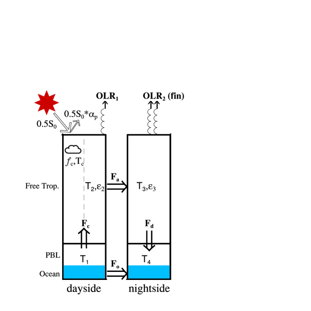
The model divides the atmosphere into two columns with one representing the dayside and the other representing the nightside (Fig. 1). This is the most basic possible simplification that allows horizontal heterogeneity, and it is justified by the following facts: (1) Only the dayside receives stellar flux from the parent star, whereas the nightside is heated by atmospheric and ocean heat import from the dayside. The temperatures of the two sides are therefore determined by distinct physical processes. (2) GCM simulations have found that on the nightside horizontal surface and air temperature gradients are extremely small and atmospheric descent occurs throughout the nightside (Joshi et al., 1997; Merlis & Schneider, 2010); therefore, the nightside atmosphere can be approximated as a single column. (3) On the dayside, the surface temperature is homogeneous in the vicinity of the substellar point in GCM simulations, and more broadly much of the dayside is characterized by robust moist convection and mean ascent (YCA13; Merlis & Schneider, 2010), so that it can be roughly treated as a single column. (4) The dayside has a moist atmosphere with a robust hydrological cycle whereas the nightside atmosphere is extremely dry (Merlis & Schneider, 2010; Edson et al., 2011). (5) Future observations of horizontal variations in the climate on tidally locked terrestrial planets are likely to be coarse, so it is reasonable to develop a model with minimal horizontal resolution.

In our model, the dayside column is thought of as a moist region with deep convection, mean ascent, and a warm surface. The air temperature follows a saturation moist adiabatic temperature profile. In this way the dayside is similar to the warm pool of the tropical Pacific Ocean on Earth, where the temperature profile is close to a moist adiabat (Xu & Emanuel, 1989). The nightside column has mean descent with dry air and a cold surface, which is analogous in some ways the subtropics of Earth. The implicit atmospheric circulation connecting the dayside and the nightside in the model approximates a global-scale Walker circulation driven by the stellar energy contrast, as obtained in GCM simulations (see the review of Showman et al. (2013)). To simulate the effect of clouds, we employ a simple convective cloud scheme and tune one free parameter of the scheme to produce a similar cloud albedo to that obtained in the GCM simulations of YCA13. At a given stellar flux and a specified ocean heat transport, the model computes dayside and nightside surface temperature, dayside and nightside free-tropospheric temperature, dayside convective heat flux, and atmospheric heat transport from the dayside to the nightside.

Figure 1.— Schematic representation of the two-column model for the climate of tidally locked terrestrial planets. The dayside column consists of a cloudy part and a clear-sky part. S₀: stellar flux at substellar point; $\alpha_{p}$: planetary albedo; $OLR$: outgoing longwave radiation (infrared emission to space); $f_{c}$: effective cloud fraction; $T_{c}$: cloud emission temperature; $\varepsilon_{2},_{3}$: atmospheric emissivity; PBL: planetary boundary layer; $F_{c}$: convective heat flux; $F_{a}$: atmospheric heat transport from dayside to nightside; $F_{o}$: ocean heat transport; and $F_{d}$: the fraction of atmospheric heat transport from the dayside to the nightside deposited in the nightside boundary layer due to adiabatic heating.

Similar types of models have been employed to investigate the climate of the tropics on modern Earth. Such models have been found to be useful for identifying the mechanisms that regulate the surface temperature of the tropical Pacific Ocean, including surface evaporation (Hartmann & Michelsen, 1993), convective clouds (Ramanathan & Collins, 1991), stratus low clouds (Larson et al., 1999), water vapor greenhouse effect (Pierrehumbert, 1995), horizontal atmospheric heat transport (Hartmann & Michelsen, 1993; Pierrehumbert, 1995), and ocean dynamics (e.g., Clement & Seager, 1999). Because of the extreme simplifications of these column models, their applicability to direct comparison with detailed and spatially dense observations is somewhat limited; however, they have significantly improved our understanding of tropical climate by helping to identify the essential processes that govern the system.

Figure 2.— GCM output that supports the weak-temperature-gradient approximation for tidally locked planets. (a) Vertical temperature profiles for a tidally locked configuration with a rotation period of 60 Earth-days. Red line: for the tropics (30^∘S–30^∘N) of the dayside; green line: for the extra-tropics of the dayside; blue line: for the entire nightside; and black line: global mean. (b) Free-tropospheric temperature contrast between dayside and nightside (mean value between the pressure levels of 100 and 600 $hPa$) as a function of rotation period. The stellar flux is 1200 W m^-2 in these simulations.

We tune our two-column model to a GCM, which fully resolves atmospheric circulation, radiative transfer, the hydrological cycle, and clouds. We use an Earth GCM, the Community Atmosphere Model version 3 (CAM3; Collins et al. (2004)), developed by the National Center for Atmospheric Research. The GCM is coupled to a mixed layer ocean with a uniform depth of 50 m. We have modified the GCM to simulate the climate of tidally locked planets around M-stars (for details, see YCA13). The default planetary radius, gravity, and rotation period are set to two times Earth’s, 13.7 m s^-2, and 60 Earth-days, respectively. The atmosphere is composed of N₂ and H₂O with a surface pressure of 1 bar, and other greenhouse gases such as CO₂, CH₄, N₂O, and O₃ are set to zero. Three groups of experiments with different stellar fluxes (from 1000 to 2400 W m^-2), ocean heat transport (from 0 to 55 W m^-2), and rotation periods (from 5 to 100 Earth-days) were performed, and the results are used here for comparisons with the two-column model. The GCM and the two-column model share the same planetary and atmospheric parameters, such as planetary gravity and specific heat of air.

The goal of this study is to increase understanding of the key controls on surface temperature and thermal emission flux of tidally locked Earth-like planets. The basic physical processes that we build into the model are outlined in Section 2. The model is developed in Section 3. Section 4 presents the behavior of the two-column model, comparisons of model results with GCM simulations, and sensitivity analyses of the model. In Section 5, the critical stellar flux at which the day–night thermal emission contrast becomes negative is addressed. This contrast is essential for the interpretation of phase curves of terrestrial planets that will be measured in the near future. Section 6 summarizes the main findings of this study.

2. Essential Physical Processes

The orbital distance of tidally locked planets in the habitable zone of M stars should be in the range of $\approx$0.02–0.2 AU (1 AU is the distance between Earth and Sun) (YCA13; Kasting et al., 1993; Kopparapu et al., 2013), corresponding to rotation periods of tens of Earth-days. The extreme variation in stellar radiation around the planet and the slow rotation rate (corresponding to a weak Coriolis force) imply that in many ways the climate of tidally locked planets will be quite different from that of Earth. Despite this, we should still be able to use basic principles of climate dynamics discovered by studying Earth to better understand the climate of these planets. In this section, we outline the essential physical mechanisms that we believe govern the climate of tidally locked terrestrial planets, including the weak-temperature-gradient approximation, a stabilizing cloud feedback, and the fixed anvil temperature hypothesis. We will also discuss the factors determining thermal emission to space.

2.1. The Weak-temperature-gradient Approximation

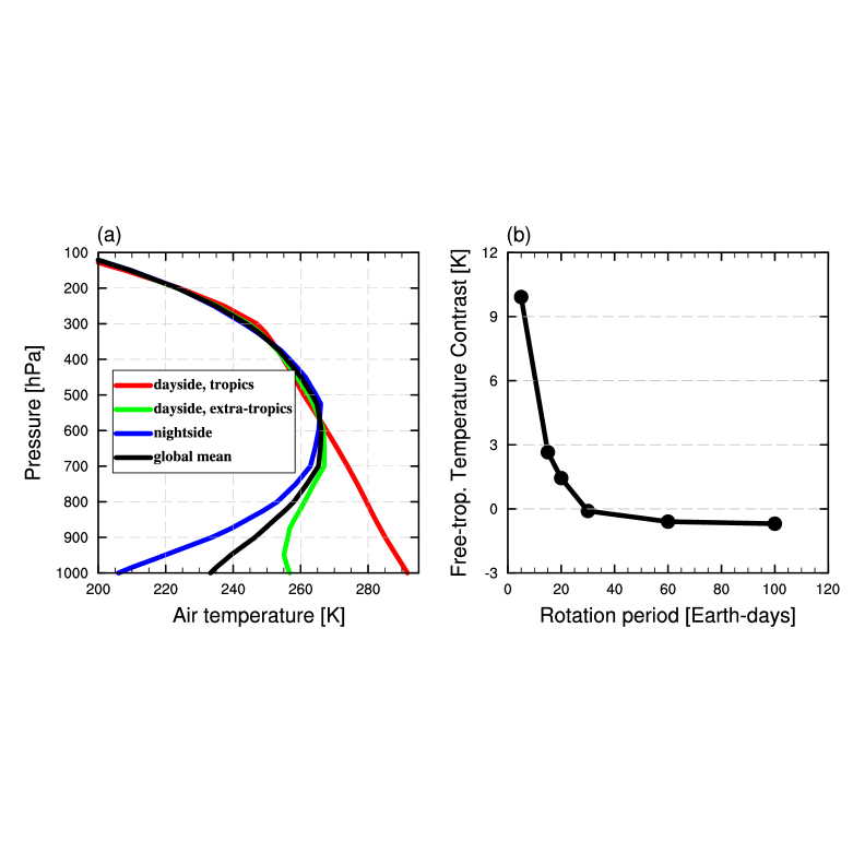
GCM simulations suggest that the free-tropospheric temperature of tidally locked habitable planets should be quite horizontally uniform (Fig. 2a) due to the weak Coriolis force. This property is similar to the condition of the tropics on Earth (Pierrehumbert, 1995; Sobel et al., 2001) where the Coriolis force is also weak, which allows the horizontal temperature gradients of the free troposphere to be approximated as zero. This is referred to as the weak-temperature-gradient (WTG) approximation. It is important to note that the WTG approximation only applies to the atmosphere above the planetary boundary layer. In the planetary boundary layer, where frictional forces become important in the momentum balance, horizontal temperature gradients can remain large, so that the nightside surface can become much colder than the dayside surface. On a tidally locked planet, where strong inversions develop on the nightside and at high latitudes on the dayside, a stably stratified planetary boundary layer can extend up to $\approx$600 hPa (see Fig. 2a). Nevertheless, a model approximating the atmosphere with just two levels, the boundary layer (and surface) and the free troposphere, can yield a faithful representation of the longitudinal variation in infrared emission to space (Mills & Abbot, 2013).

Figure 3.— GCM output justifying the fixed anvil temperature hypothesis for tidally locked planets. (a) Dayside ice cloud water content, and (b) normalized clear-sky longwave heating rate, as a function of air temperature. The horizontal gray bold line roughly shows the temperature at the top of ice clouds where a sharp decrease in the clear-sky longwave heating rate occurs. Note that the pressure at which $T$ = 230 $K$ occurs is $\approx$150, 100, 40 and 12 $hPa$ for the stellar fluxes of 1400, 1600, 1800, and 2000 W m^-2, respectively.

The weak temperature gradient in the free troposphere can be brought about by a variety of physical processes. Temperature gradients set up gravity waves that quickly diminish them. Additionally, the atmospheric circulation of tidally locked planets is characterized by a global-scale Walker circulation: strong updrafts near the substellar point, divergence at high altitudes, broad downwelling at the entire nightside, and convergence flows at low altitudes, returning to the substellar region (Showman et al., 2013). Moreover, the zonal-mean zonal wind velocity is dominated by a weak eastward superrotation along the equator. This equatorial superrotation results from equatorward zonal momentum transport by Rossby waves induced by strong zonal variations in the stellar radiation (e.g., Showman & Polvani, 2011). All of these processes are important for transporting heat from dayside to nightside and maintaining the weak temperature gradient in the troposphere.

The WTG approximation is not valid if the timescale for atmospheric heat transport is longer than the radiative timescale. Two ways for this to happen are if the planet has a small orbital (and rotational) period or has an extremely hot and/or thin atmosphere (Perez-Becker & Showman, 2013). For our sample GCM simulations the largest horizontal temperature differences in the free troposphere around the planet are only $\approx$10 K when the orbital period is 5 Earth-days (Fig. 2b). This is consistent with previous work indicating that the WTG approximation does a good job of approximating the temperature profile of a tidally locked planet even if the rotation period is only 1 Earth-day (Merlis & Schneider, 2010; Mills & Abbot, 2013), and suggests that the WTG approximation may be more broadly applicable than one might initially suspect.

2.2. The Stabilizing Cloud Feedback

Clouds contribute most of the planetary albedo of Earth (Donohoe & Battisti, 2011). Consistent with the global-scale Walker circulation and ascent at the substellar region, most parts of the dayside of tidally locked Earth-like planets would be covered by water clouds (YCA13; Edson et al., 2011), which would greatly increase the planetary albedo and dramatically cool the planet. The cloud albedo effect becomes stronger as the planet is moved closer to its parent star because higher stellar insolation drives stronger convection, producing more clouds and increasing their optical depth. This stabilizing cloud feedback significantly delays the onset of a runaway greenhouse state as the stellar flux increases and therefore shifts the inner edge of the habitable zone substantially toward its star (YCA13).

In the two-column model, we parametrize convection as a vertical mixing of moist static energy (MSE) between the boundary layer and the free troposphere. Convection commences when the boundary-layer MSE exceeds the free-tropospheric saturation MSE (Raymond, 1995). The cloud fraction and cloud albedo are assumed to be proportional to the logarithm of the convective heat flux, as suggested by observations of tropical convective clouds on Earth (Slingo, 1980). The logarithm formula connects the optical properties of clouds to the strength of convection, and enables the model to capture the effect of the stabilizing cloud feedback.

2.3. The Fixed Anvil Temperature Hypothesis

Figure 4.— GCM simulated outgoing longwave radiation at the top of the atmosphere on the dayside (solid line) and on the nightside (dashed line) as a function of the stellar flux ($S_{0}$). (a) Clear-sky conditions without clouds, and (b) all-sky conditions including the effect of clouds. Note (a) and (b) are calculated with the same surface temperatures, air temperatures, and water vapor concentrations.

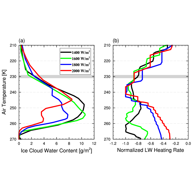
Studies of tropical anvil clouds on Earth suggest that their emission temperature is nearly constant as the climate changes. This is referred to as the fixed anvil temperature (FAT) hypothesis (Hartmann & Larson, 2002). Energy balance in the tropical troposphere is primarily between convective heating by latent heat release in regions of deep convection and radiative cooling by longwave emission to space in clear-sky regions (i.e., the regions without clouds) with large-scale subsidence. Because of this, the detrainment level (where outflow occurs) of anvil clouds should be located at the altitude where the clear-sky radiative cooling diminishes rapidly. The clear-sky radiative cooling rate in the upper troposphere is primarily determined by water vapor emission. The temperature at which the saturation water vapor pressure becomes small enough that water vapor emission is ineffective is narrowly constrained by local air temperature because of the Clausius–Clapeyron relation, and does not depend on surface temperature. The FAT hypothesis asserts that the temperature at which anvil clouds detrain is determined by the level where a large decrease in water vapor radiative cooling occurs. According to the FAT hypothesis, the temperature at the top of anvil clouds should be nearly independent of surface temperature, which exerts a strong constraint on the strength of cloud longwave forcing.

Recent simulations with cloud-resolving models (e.g., Kuang & Hartmann, 2007) and analyses with cloud object data (e.g., Li et al., 2012) support the FAT hypothesis. Furthermore, Zelinka & Hartmann (2010) show that the cloud-top temperature in GCMs with parameterized clouds also remain approximately constant as greenhouse gas concentrations are increased. Our GCM simulations of tidally locked planets also support the FAT hypothesis. As shown in Fig. 3, the clear-sky cooling rate decreases rapidly at a constant air temperature, and the cloud-top temperature stays constant when the stellar flux is increased massively. In the two-column model, it is therefore reasonable to set the cloud-top temperature to a constant.

2.4. Factors Determining Thermal Emission to Space

A primary tool for deciphering the climate of terrestrial exoplanets will be to examine phase variations in their infrared emission flux, commonly referred to as outgoing longwave radiation in Earth science ($OLR$). The $OLR$ is primarily determined by surface temperature ($T_{s}$), air temperature ($T_{a}$), atmospheric specific humidity ($q$, the mass ratio of water vapor to dry air), and clouds. Changes in temperature and humidity have opposing effects on $OLR$: increases in $T_{s}$ and $T_{a}$ increase $OLR$, while increases in $q$ decrease $OLR$ due to the water vapor greenhouse effect (Pierrehumbert, 2010). Clouds can also significantly reduce $OLR$ (Ramanathan et al., 1989). $OLR$ can be thought of as the sum of surface upward emission which survives absorption by water vapor, reemission from the atmosphere, and a negative term due to cloud absorption,

$$OLR=(1-\varepsilon(q))\sigma T_{s}^{4}+\varepsilon(q)\sigma T_{a}^{4}-C_{l},$$ (1)

where $\varepsilon(q)$ is the clear-sky atmospheric infrared emissivity as a function of specific humidity ($q$), $C_{l}$ is the cloud longwave forcing (i.e., the change in $OLR$ in the presence of clouds relative to the clear-sky condition), and $\sigma$ is the Stefan-Boltzmann constant. For an optically thin clear-sky atmosphere, $\varepsilon$ is close to zero, and $OLR$ is close to the surface emission. For an optically thick clear-sky atmosphere, $\varepsilon$ is close to one, and $OLR$ is primarily determined by the emission from the upper levels of the atmosphere.

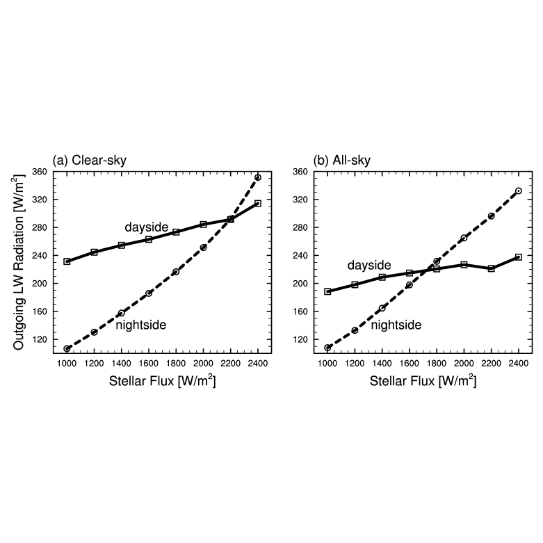
For tidally locked terrestrial planets, the dayside specific humidity tends to be higher than the nightside specific humidity at all atmospheric levels. This is because the relative humidity tends to be higher at all levels on the dayside, and additionally the dayside temperature is much higher in the boundary layer. As a result, the rate of increase of the dayside clear-sky $OLR$ with stellar flux is much smaller than that on the nightside (Fig. 4a). The high water vapor concentration shifts the atmospheric emission level to higher altitudes with colder temperatures, which keeps the dayside $OLR$ from increasing much.

The dayside is covered by high-level clouds which strongly reduce the dayside OLR whereas the nightside is dominated by low-level clouds that have little effect on the nightside OLR. High-level clouds absorb thermal emission from the warm surface and reemit it to space following the Stefan–Boltzmann law at the temperature of the cloud, which is much lower than the surface temperature, reducing $OLR$. Low-level clouds have nearly zero effect on $OLR$ because they have temperatures close to the surface temperature. GCM simulations show that as a result of the global circulation pattern, with ascent on the dayside and descent on the nightside, the dayside should be covered by both high-level and low-level clouds while the nightside should be dominated by low-level clouds (Fig. 1 of YCA13) that form when water vapor is trapped in the boundary layer under the temperature inversion (see Fig. 2a). Because of the combined effect of clouds and water vapor, the dayside all-sky (including clouds) $OLR$ is nearly constant as the stellar flux is varied (Fig. 4b).

In our two-column model, the clear-sky region of the atmosphere is treated as an equivalent gray gas atmosphere characterized by an emissivity that is a function of water vapor content (Pierrehumbert, 2010). This representation qualitatively captures the greenhouse effect of water vapor without requiring detailed calculations of the radiative transfer. In order to calculate the cloud longwave forcing, the dayside column also includes a cloudy region that emits at a constant temperature (following the FAT hypothesis). This scheme does a reasonable job of simulating the cloud longwave effect.

3. The Two-column Model

In this section, we construct an idealized two-column model (shown schematically in Fig. 1) that incorporates all the physical processes addressed in Section 2 above. The dayside column is thought of as a region with deep convection, net ascent, and a moist atmosphere. The nightside column has no convection and represents a dry region of mean descent. In each column, the upper level represents the free troposphere and the lower level represents both the boundary layer and the surface. The boundary layer and surface are assumed to be tightly coupled by turbulent mixing and therefore have approximately the same temperature. The dayside free troposphere has two parts, the clear-sky part and the cloudy part.

The model is formulated by requiring energy balance in the free troposphere and at the surface (Eqs. (2–5)), making the WTG approximation (Eq. (6)), enforcing convective neutrality on the dayside (Eq. (7)), and assuming the FAT hypothesis is correct (Eq. (8)). The model equations are:

$$\frac{1}{2}S_{0}(1-\alpha_{p})-F_{c}-F_{o}+(1-f_{c})\varepsilon_{2}\sigma T_{2}^{4}+f_{c}\sigma T_{c}^{4}-\sigma T_{1}^{4}=0,$$ (2)

$$F_{c}-F_{a}+(1-f_{c})\varepsilon_{2}\sigma T_{1}^{4}+f_{c}\sigma T_{1}^{4}-2(1-f_{c})\varepsilon_{2}\sigma T_{2}^{4}-2f_{c}\sigma T_{c}^{4}=0,$$ (3)

$$F_{a}-F_{d}+\varepsilon_{3}\sigma T_{4}^{4}-2\varepsilon_{3}\sigma T_{3}^{4}=0,$$ (4)

$$F_{o}+F_{d}+\varepsilon_{3}\sigma T_{3}^{4}-\sigma T_{4}^{4}=0,$$ (5)

$$T_{2}-T_{3}=0,$$ (6)

$$MSE_{1}=MSE_{2}^{*},$$ (7)

$$T_{c}=230.$$ (8)

Here, $T_{1}$ and $T_{4}$ are the surface temperatures of the dayside and nightside, respectively; $T_{2}$ and $T_{3}$ are the free-tropospheric temperatures of the dayside and nightside, respectively; $T_{c}$ is the cloud emission temperature; $S_{0}$ is the stellar flux at the substellar point and $\frac{1}{2}$$S_{0}$ is the stellar flux impinging on the dayside surface (averaged over the stellar zenith angle); $\alpha_{p}$ is the planetary albedo; $F_{c}$ is the convective heat flux from the boundary layer to the free troposphere in the dayside column; $F_{a}$ and $F_{o}$ represent atmospheric and ocean heat transports from dayside to nightside, respectively; $F_{d}$ is the adiabatic heating due to dry descent in the nightside column; $\varepsilon_{2}$ and $\varepsilon_{3}$ are the free tropospheric emissivities of the dayside and nightside, respectively; $f_{c}$ is the effective cloud fraction; $MSE_{1}$ is the dayside surface moist static energy; and $MSE_{2}^{*}$ is the dayside free-tropospheric saturation moist static energy. Using the six Equations (2–7), we are able to determine solutions for the six dependent variables of the model: surface temperature ($T_{1}$ & $T_{4}$), free tropospheric temperature ($T_{2}$ & $T_{3}$), atmospheric heat transport ($F_{a}$), and dayside convective heat flux ($F_{c}$). This solution is a function of the independent variables: the strength of stellar flux ($S_{0}$), ocean heat transport ($F_{o}$), and model parameters.

Following the WTG approximation, the atmospheric energy transport ($F_{a}$) is forced to be strong enough to drive the dayside and nightside free-tropospheric temperature together (Eq. (6)). This approximation allows the details of atmospheric dynamics to be avoided but retains the net effect of atmospheric dynamics on the air temperature. We assume that some of $F_{a}$, the total atmospheric heat transport from the dayside to the nightside, is deposited in the boundary layer ($F_{d}$) and the rest is deposited in the free troposphere ($F_{a}-F_{d}$). We take $F_{d}$ to be

$$F_{d}=k_{1}F_{a},$$ (9)

where $k_{1}$ is a constant parameter (see Table 1).

The surface and clouds are assumed to emit like blackbodies (i.e., $\varepsilon$ $=$ 1). The free troposphere is assumed to radiate as an equivalent gray body with emissivities of $\varepsilon_{2}$ and $\varepsilon_{3}$, determined by water vapor concentration

$$\varepsilon_{2},_{3}=1.0-\exp(-\frac{\varkappa\,P_{a}}{g}\,q_{2},_{3})=1.0-\exp(-k_{2}\,q_{2},_{3}),$$ (10)

where $q_{2}$ and $q_{3}$ are specific humidities of the dayside and nightside respectively, $\varkappa$ is an absorption coefficient, $q$ is the specific concentration of water vapor, $P_{a}$ is the air pressure, and $g$ is the acceleration due to gravity, and $k_{2}$ is a constant coefficient with $k_{2}\equiv\varkappa\,P_{a}/g$. Equation (10) follows from the gray gas approximation (e.g., Pierrehumbert (2010)), and is similar to that employed in Emanuel (2002). We calculate the specific humidity by assuming fixed relative humidities ($RH_{2}$ and $RH_{3}$, the ratio of water vapor partial pressure to saturation water vapor partial pressure) and calculating the saturation water vapor partial pressure using the Clausius-Clapeyron relationship. By the Clausius-Clapeyron relationship, saturation water vapor partial pressure is roughly exponential in air temperature, increasing $\approx$7% for each 1 K in temperature at Earth-like temperatures (Emanuel, 1994). An additional term in Eq. (10) could be easily added to account for the change of optical thickness due to atmospheric CO₂ absorption (for example, see Emanuel (2002)).

Table 1Model parameters used for the reference climate calculations.

Parameter	Description	Value
$P_{a}$	the depth of convection	600 $hPa$
$T_{c}$	the cloud emission temperature	230 $K$
$RH_{1}$	relative humidity of the dayside boundary layer	90%
$RH_{2}$	relative humidity of the dayside free troposphere	80%
$RH_{3}$	relative humidity of the nightside free troposphere	30%
$k_{1}$	fraction of heat transport to the nightside	0.2
	deposited in the boundary layer (Eq. (9))
$k_{2}$	relates water vapor to the infrared opacity (Eq. (10))	1000
$k_{3}$	relates convection to the cloud fraction (Eq. (13))	0.08

Figure 5.— Reference climate solution of the two-column model as a function of stellar flux ($S_{0}$) compared with output from the GCM CAM3. Lines represent the results of the two-column model, and squares and circles represent those of the GCM CAM3. (a) dayside surface temperature ($T_{1}$); (b) nightside surface temperature ($T_{4}$); (c) planetary albedo ($\alpha_{p}$); (d) dayside cloud longwave forcing ($C_{l}$); (e) outgoing longwave radiation on the dayside ($OLR_{1}$) and on the nightside ($OLR_{2}$); and (f) atmospheric heat transport from dayside to nightside ($F_{a}$). Model parameters are listed in Table 1. The squares and circles in (e) are the same as those in Fig. 4(b) for comparison.

The convective heat flux ($F_{c}$) is determined implicitly by requiring convective neutrality, which can be approximated by requiring that the boundary layer moist static energy equals the free-tropospheric saturation moist static energy (Abbot & Tziperman, 2009). The moist static energy of the surface is

$$MSE_{1}=C_{p}T_{1}+Lq_{1},$$ (11)

while the free-tropospheric saturation moist static energy is

$$MSE_{2}^{*}=C_{p}T_{2}+Lq_{2}^{*}+gZ_{a},$$ (12)

where $C_{p}$ is the specific heat of the air at constant pressure ($C_{p}$ = 1005.7 $J\,kg^{-1}\,K^{-1}$), $L$ is the latent heat of evaporation ($L$ = 2.501$\times$10⁶ $J\,kg^{-1}$), $q_{1}$ is the surface specific humidity, $q_{2}^{*}$ is the free-tropospheric saturation specific humidity, $g$ is the planetary gravitational acceleration, and $Z_{a}$ is the height of convection, which we take to be a constant.

We set the relative humidity of the dayside free troposphere, $RH_{2}$, to 80% and of the nightside free troposphere, $RH_{3}$, to 30%, roughly the mean values we obtain from CAM3 simulations over a variety of stellar fluxes. Similarly, we set the dayside boundary layer relative humidity, $RH_{1}$, to 90%. We calculate the height of convection, $Z_{a}$, by specifying the pressure of the free tropospheric layer, $P_{a}$, and assuming a scale height of 5000 $m$. This scale height is smaller than that of Earth, $\approx$7500 $m$, due to the fact that we use a larger gravitational acceleration (13.7 versus 9.8 $m\,s^{-2}$).

Figure 6.— As in Fig. 5, but as a function of ocean heat transport from dayside to nightside ($F_{o}$). The stellar flux is 1200 W m^-2 in these calculations. Model parameters except for the parameter varied ($F_{o}$), are the same as those for the reference climate calculations (Table 1). The moderate differences between the two-column model and GCM are due to the difference in the base state with $F_{o}$=0 (Fig. 5), and can be removed by changing either the parameter $k_{1}$ or $k_{2}$ slightly.

A simple convective cloud scheme is employed to describe the cloud behavior. The effective cloud fraction ($f_{c}$) is related to the convective heat flux ($F_{c}$) with an upper limit of 1.0

$$f_{c}=min(k_{3}\ln(F_{c}+1.0),1.0),$$ (13)

where $k_{3}$ is an adjustable parameter that we set to $k_{3}$ = 0.08 by tuning the model to roughly reproduce cloud albedos obtained in CAM3 simulations. This logarithmic scheme for convective clouds was proposed by Xu & Krueger (1991) and used to parameterize the cloud fraction in CAM3 (Collins et al., 2004) and its recently released versions, CAM4 (Neale et al., 2010a) and CAM5 (Neale et al., 2010b), and it is able to roughly simulate the convective cloud coverage over the tropics of Earth (Hack et al. 2006). We assume that the nightside column is cloud-free because clouds there can have no albedo effect and have a small greenhouse effect because they are near the surface.

Cloud albedo depends on both cloud fraction and cloud microphysics. For simplicity, detailed microphysical descriptions (Kitzmann et al., 2010; Zsom et al., 2012) are not included in the model, and we assume that the cloud albedo equals one where there are clouds. Using this assumption, the planetary albedo ($\alpha_{p}$), determined by the combined effect of surface and cloud albedos, is

$$\alpha_{p}=0.09+f_{c}-0.09\times f_{c},$$ (14)

where 0.09 is the albedo of seawater averaged over the dayside (including the dependence of albedo on the stellar zenith angle). If there are no clouds, the planetary albedo is equal to the seawater albedo. We do not include the contribution of sea ice and snow to the planetary albedo, which would only be relevant near the outer edge of the habitable zone when significant amounts of sea ice and snow spread to the dayside.

We specify the cloud emission temperature ($T_{c}$) to be a constant in accordance with the FAT hypothesis. We set $T_{c}$ = 230 K, which is the value suggested by our GCM simulations (see Fig. 3) and is 12 K higher than that of tropical anvil clouds of Earth ($\approx$218 K; Houze & Betts, 1981).

We neglect a variety of physical processes in the model. For example, we do not consider shortwave absorption by water vapor and clouds, feedbacks due to changes of convection depth and relative humidity, the detailed interaction between atmospheric and oceanic circulations, and the momentum and moisture budgets. Despite these simplifications, the low-order two-column model is able to capture many of the fundamental features of the GCM simulations.

4. Reference Climate and Model Sensitivity

In this section, we first show that it is possible to tune the two-column model to reproduce the results of the GCM CAM3 simulations. Next, we investigate the sensitivity of the model to increases in ocean heat transport, cloud radiative forcing, and atmospheric emissivity.

4.1. Reference Climate

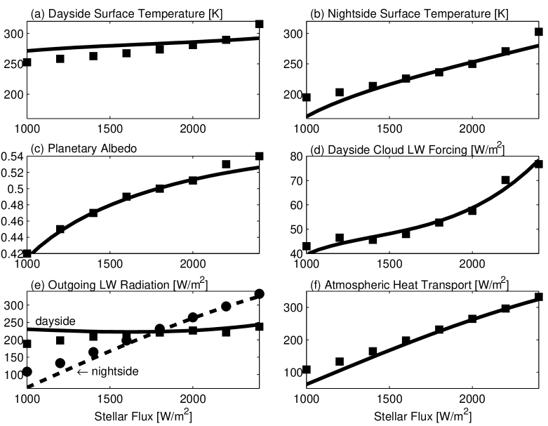
We plot model variables at steady state for the reference climate as a function of stellar flux in Fig. 5 (see Table 1 for model parameters). The ocean heat transport is set to zero in these calculations. We choose the values of $P_{a}$, $T_{c}$, $RH_{1}$, $RH_{2}$, and $RH_{3}$ by averaging equivalent variables in the CAM3 GCM simulations. We then tune the two-column model to CAM3 by adjusting only three parameters: $k_{1}$, $k_{2}$, and $k_{3}$. When the two-column model is tuned to CAM3 in this way, it is able to capture the fundamental features of the climate, including surface temperature, planetary albedo, cloud longwave forcing, thermal emission flux, and atmospheric heat transport.

Both the dayside and nightside surface temperatures increase as the stellar flux increases, and their magnitudes are close to CAM3’s. The planetary albedo of the two-column model behaves very similarly to that of CAM3, which shows that our simple convective cloud scheme is capable of capturing the bulk effects of cloud albedo on the climate. The planetary albedo of tidally locked terrestrial planets (between 0.42 and 0.54) is much higher than that of Earth ($\approx$0.3). This results from a high cloud fraction near the substellar point, where the stellar flux is highest (YCA13). The two-column model also has very similar dayside cloud longwave forcing to that of CAM3 (between 40 and 80 W m^-2).

As the stellar flux increases, both models predict that the dayside thermal emission flux is nearly constant whereas the nightside thermal emission increases rapidly (Fig. 5e). When the stellar flux is higher than $\approx$1800 W m^-2, the thermal emission flux on the nightside exceeds that on the dayside. The strength of atmospheric heat transport from dayside to nightside is quite similar between the two-column model and CAM3 (Fig. 5f), confirming the accuracy of the WTG approximation.

Figure 7.— Sensitivity of global-mean surface temperature ($\frac{T_{1}+T_{4}}{2}$) to cloud albedo and cloud longwave forcing, as a function of stellar flux ($S_{0}$). Solid line: with both effects; dashed-dotted line: no cloud albedo effect ($\alpha_{p}$ = 0.09); dotted line: no cloud greenhouse effect ($C_{l}$ = 0); and dashed line: planetary albedo and cloud greenhouse effect are fixed to those at a stellar flux of 1000 W m^-2 ($\alpha_{p}$ = 0.415, $C_{l}$ = 40 W m^-2; i.e., no cloud feedback). Other model parameters are the same as those for the reference climate calculations (Table 1).

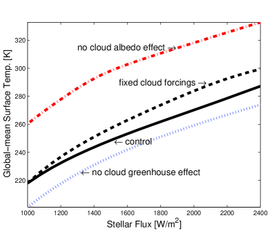
Figure 5 shows that as the stellar flux increases, the nightside surface temperature increases much faster than the dayside surface temperature. The main reason for this is that the atmosphere efficiently transports energy absorbed on the dayside to the nightside (Fig. 5f).

These comparisons between the two-column model and CAM3 demonstrate that despite of the simplicity of our assumptions, the two-column model is able, when appropriately tuned, to reproduce the main climate features of tidally locked terrestrial planets as simulated by a GCM. This indicates that the climate of tidally locked planets is well described by the handful of essential physical processes contained in the two-column model.

4.2. The Effect of Ocean Heat Transport

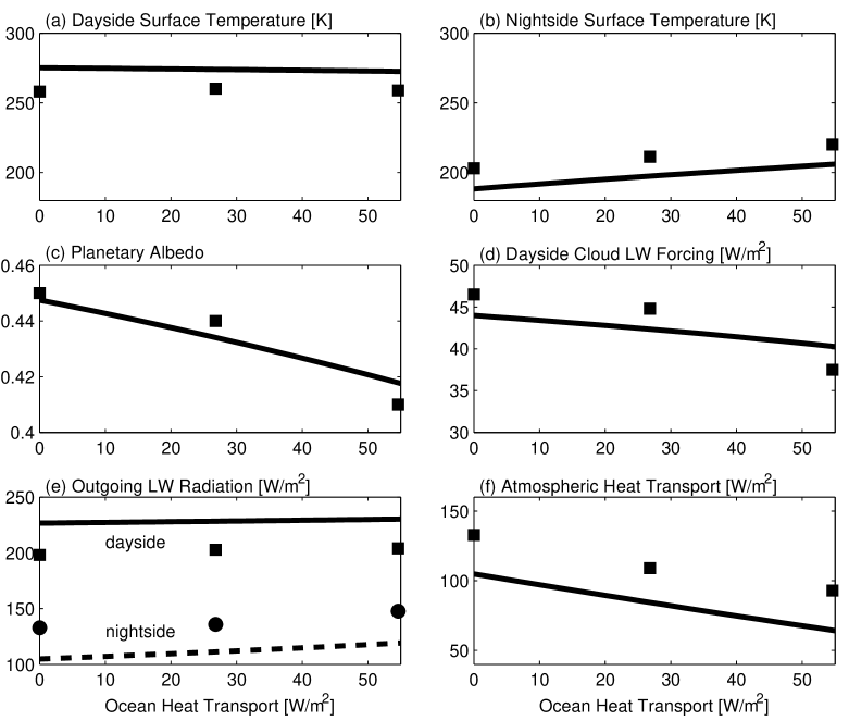
Here we investigate how the climate responds to imposed ocean heat transport from dayside to nightside. To investigate this we performed a series of calculations in which the ocean heat transport is varied while the stellar flux is fixed to a constant (Fig. 6). As the ocean heat transport is increased, the dayside surface temperature decreases slightly while the nightside surface temperature increases significantly, so that the global-mean surface temperature increases, and the surface temperature and thermal emission contrasts between dayside and nightside decrease. Both the planetary albedo and the cloud longwave forcing decrease because increasing ocean heat transport decreases the day–night surface temperature contrast, weakening the convergence and convection on the dayside. The atmospheric heat transport decreases in response to the increase in ocean heat transport, such that the total heat transport shows a small increase. This compensation between the atmosphere and ocean is consistent with the results of simulations with a fully coupled 3D atmosphere-ocean circulation model (Hu & Yang, 2014) and is similar to the behavior that meridional atmospheric and ocean heat transports on Earth are believed to exhibit (Stone, 1978; Farneti & Vallis, 2013).

We tuned the two-column model to the GCM over a range of stellar fluxes, and it deviates somewhat from the GCM when the ocean heat transport is zero at the particular stellar flux for which we varied the ocean heat transport in the GCM (Fig. 6). Nevertheless, the two-column model does a good job of reproducing the trends of the GCM as the ocean heat transport is increased. Moreover, by slightly changing $k_{1}$ or $k_{2}$ we can greatly improve the match between the GCM and the two-column model when the ocean heat transport is varied at this particular stellar flux (not shown).

The fact that the two-column model can roughly reproduce the behavior of the GCM when ocean heat transport is varied, even though it was tuned to match the GCM when stellar flux is varied, suggests that the approximations we have made capture the relevant physics, rather than the model simply being cleverly tuned. For example, the fact that the response of atmospheric heat transport to changes in ocean heat transport in the two-column model is very similar to that in the GCM emphasizes the validity of the WTG approximation. Furthermore, the similar changes in planetary albedo and cloud longwave forcing between the models suggests that the convective scheme and FAT hypothesis are faithful representations of the more complete physics contained in the GCM.

Figure 8.— Sensitivity of the climate to atmospheric emissivity of dayside ($\varepsilon_{2}$) and nightside ($\varepsilon_{3}$). Left panels: dayside surface temperature ($T_{1}$); right panels: atmospheric heat transport from dayside to nightside ($F_{a}$). (a) & (b): Varying $\varepsilon_{2}$ but fixed $\varepsilon_{3}$ to 0.5; (c) & (d): varying $\varepsilon_{3}$ but fixed $\varepsilon_{2}$ to 0.5. The stellar flux is 2400 W m^-2. Planetary albedo and cloud longwave forcing are fixed ($\alpha_{p}$ = 0.415, $C_{l}$ = 40 W m^-2). Other model parameters are the same as those for the reference climate calculations.

4.3. The Importance of Cloud Albedo Effect

Clouds have significant effects on the climate of tidally locked planets (YCA13). In order to further establish the importance of clouds, we performed calculations with either the cloud albedo or cloud longwave forcing set to zero (Fig. 7). For the no cloud albedo effect experiment, Eq. (14) is not used and the planetary albedo is set to equal to the seawater albedo (0.09). For the no cloud longwave effect experiment, Eq. (13) is not used and the cloud longwave forcing is set to zero.

Comparisons with the reference climate experiments show that the global-mean surface temperature decreases by $\approx$15 K for the no cloud longwave effect experiments while it increases by $\approx$40 K if the cloud albedo effect is turned off. This indicates that the cloud albedo cooling effect is much stronger than the cloud greenhouse warming effect. The net effect of the clouds is therefore to dramatically cool the planet, delaying the onset of a runaway greenhouse, as addressed in YCA13.

We also performed a series of calculations with a fixed planetary albedo of 0.415 and a fixed cloud longwave forcing of 40 W m^-2, which are their values when the stellar flux is equal to 1000 W m^-2. These calculations investigate the model with clouds, but without a cloud feedback (changes in cloud forcing as a function of climate). The dashed line of Fig. 7 shows that the surface temperature increases by $\approx$15 K on the dayside, relative to the interactive cloud case, when the stellar flux is 2400 W m^-2. The cloud albedo feedback therefore has a significant cooling effect on the planet.

4.4. The Importance of the Nightside Radiator Fin

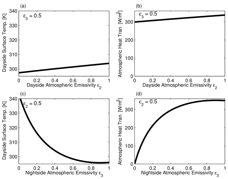
Atmospheric emissivity affects the strength of the greenhouse effect and the efficiency of infrared energy loss to space. We perform a set of experiments to test the sensitivity of the climate to atmospheric emissivity. In these experiments, Eq. (10) is not used, and instead atmospheric emissivity is set to a series of values from zero to one. The cloud radiative forcing is fixed in order to focus on the role of atmospheric emissivity.

Figure 8a shows the dayside surface temperature as a function of the dayside atmospheric emissivity ($\varepsilon_{2}$). In these experiments, the nightside atmospheric emissivity ($\varepsilon_{3}$) is fixed to 0.5. As $\varepsilon_{2}$ is increased, the dayside atmospheric greenhouse effect increases, and consequently the surface temperature increases. The magnitude of the increase, however, is small even when $\varepsilon_{2}$ is increased from zero to one. This is due to an increase in atmospheric heat export to the nightside (Fig. 8b), which warms the nightside and weakens the increase in the dayside surface temperature.

Figure 8c shows the sensitivity of the climate to varying the nightside atmospheric emissivity ($\varepsilon_{3}$). In these experiments, the dayside atmospheric emissivity ($\varepsilon_{2}$) is fixed to 0.5. As $\varepsilon_{3}$ is increased, the dayside surface temperature decreases strongly, although the nightside and global-mean surface temperatures increase (not shown). As $\varepsilon_{3}$ is increased from zero to 1.0, the dayside surface temperature decreases by $\approx$45 K. As $\varepsilon_{3}$ is increased, the efficiency of the atmospheric infrared energy loss to space increases, which requires a great increase in atmospheric heat transport from dayside to nightside (Fig. 8d), therefore cooling the dayside surface.

Figure 9.— The effect of the radiator fin on the global-mean surface temperature. The one-column model (without the radiator fin) has the same parameters of the two-column model (including the radiator fin), including planetary albedo ($\alpha_{p}$ = 0.415), cloud longwave forcing ($C_{l}$ = 40 W m^-2), relative humidity, and atmospheric emissivity (Table 1).

We can draw an important physical lesson from these experiments: the nightside acts like a “radiator fin”, similar to the subtropics of Earth (Pierrehumbert, 1995), only more pronounced. All the stellar energy is deposited on the dayside and the water vapor and cloud greenhouse effects prevent the atmosphere from getting rid of all this energy locally. Much of the energy is instead transported by the atmosphere to the nightside where the air is dry, there is a strong temperature inversion, and the cloud greenhouse effect is negligible, so that infrared energy is easily emitted to space (as it would be by a “radiator fin”). The nightside atmosphere therefore has a stabilizing effect on the climate of the planet.

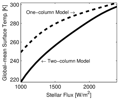
The radiator-fin effect cannot be captured in a single column model, even a 1D radiative-convective model with an extremely sophisticated radiative transfer scheme, because it requires horizontal heat transport to connect the moist and dry regions. In order to demonstrate this, we construct a one-column model with the same parameters as the two-column model. A comparison of the surface temperature as a function of the stellar flux in the one-column and two-column models is shown in Fig. 9. We find that the surface temperature of the one-column model is $\approx$15–30 K higher than the two-column model because the one-column model is not able to capture the effect of the radiator fin. The radiator-fin effect becomes weak at high stellar fluxes because the atmospheric emissivities of both the dayside and nightside approach one. This is a limitation of the simple radiative scheme in our model. Further investigation of the effect of the radiator fin on the runaway greenhouse will require a 2D or 3D model with a more sophisticated radiative scheme.

5. Day–night Thermal Emission Contrast

YCA13 proposed that cloud behavior on tidally locked terrestrial planets near the inner edge of the habitable zone would cause higher infrared thermal emission from the nightside than the dayside. This would lead to a reversal in the thermal phase curve, which is a qualitatively different signal than would normally be expected. In this section, we consider the difference in thermal emission flux between dayside and nightside in the two-column model, and show how basic physical parameters may affect this signal.

In a steady state, the dayside column heat budget can be obtained by summing Eqs. (2) and (3),

$$\frac{1}{2}S_{0}(1-\alpha_{p})-F_{a}-F_{o}=OLR_{1}.$$ (15)

$OLR_{1}$ is the thermal emission flux from the dayside, with

$$OLR_{1}=(1-\varepsilon_{2})\sigma T_{1}^{4}+\varepsilon_{2}\sigma T_{2}^{4}-C_{l},$$ (16)

where the sum of the first and second terms of the right hand side is the outgoing infrared emission in clear-sky conditions, and the third term is the reduction of the outgoing infrared emission due to the presence of clouds with

$$C_{l}=f_{c}((1-\varepsilon_{2})\sigma T_{1}^{4}+\varepsilon_{2}\sigma T_{2}^{4})-f_{c}\sigma T_{c}^{4}.$$ (17)

Figure 10a shows the three terms of Eq. (16) in the reference climate experiments. Surface emission reaching the top of the atmosphere decreases greatly with increasing stellar flux although the surface temperature increases. This is due to the increase of atmospheric absorption. Water vapor concentration increases rapidly with air temperature because of the strong temperature dependence of saturation water vapor pressure following the Clausius–Clapeyron relation, reducing the thermal emission to space. Emission by the atmosphere increases with increases in stellar flux due to increases of the air temperature ($T_{2}$) and atmospheric emissivity ($\varepsilon_{2}$). The cloud longwave effect decreases with increasing stellar flux, also reducing the thermal emission to space. The cloud effect is comparable to that of water vapor. Due to the combined effect of water vapor and clouds, the dayside $OLR$ curve as a function of the stellar flux is very flat. Figure 10a also shows that if the stellar flux is low, the optical depth of the atmosphere is small, and $OLR_{1}$ is close to the unmodified upward radiation from the surface. If the stellar flux is high, the surface upward emission is blocked by the optically thick atmosphere, and the outgoing thermal emission is primarily determined by the upper tropospheric temperature.

Figure 10.— Dayside (a) and nightside (b) thermal emission fluxes as a function of the stellar flux ($S_{0}$) between 1000 and 2400 W m^-2. Solid line: thermal emission flux to space, which has to be equal to the sum of other terms (see Eqs. (16) & (19)); dashed line: surface upward emission minus the absorption by water vapor; dashed–dotted line: atmospheric reemission; and dotted line: the effect of clouds. Model parameters are the same as those for the reference climate calculations (Table 1).

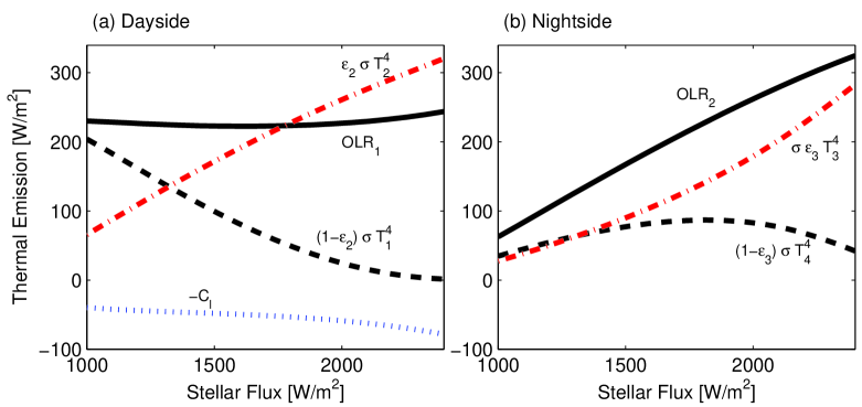
For the thermal emission flux on the dry nightside, water vapor has a small effect, and low-level clouds there have nearly zero effect. The nightside column heat budget can be obtained by summing Eqs. (4) and (5),

$$F_{a}+F_{o}=OLR_{2},$$ (18)

where $OLR_{2}$ is the thermal emission flux to space:

$$OLR_{2}=(1-\varepsilon_{3})\sigma T_{4}^{4}+\varepsilon_{3}\sigma T_{3}^{4}.$$ (19)

This means that the thermal emission flux on the nightside is equal to the sum of heat transports from the dayside by the atmosphere and ocean. Figure 10b shows the two terms of $OLR_{2}$ as a function of stellar flux. As the stellar flux increases, surface emission reaching the top of the atmosphere first increases due to the increase in surface temperature, and then decreases due to the increase of water vapor absorption. Atmospheric emission increases with increasing stellar flux due to increases of air temperature and emissivity. The net effect of the two terms is a strong increase in the thermal emission flux with increasing stellar flux.

If we assume a saturated atmosphere on the dayside, there will exist an upper limit for $OLR_{1}$ at which the atmosphere becomes optically thick at all infrared wavelengths (Kasting et al., 1993). The limit is $\approx$280 W m^-2 for planets with pure water atmospheres, Earth’s gravity, and no clouds (Goldblatt et al., 2013). If clouds are further considered, the limit will be lower. On the nightside, thermal infrared energy is more easily emitted to space through the radiator fin.

A remaining question is: What is the critical stellar flux ($S_{c}$) at which the dayside outgoing thermal emission flux becomes equal to or less than that of the nightside, i.e., $OLR_{1}$$\leq$$OLR_{2}$? If $OLR_{1}$ is higher than $OLR_{2}$, the phase curve maximum should occur when the dayside of the planet is facing the observer. If $OLR_{1}$ is lower than $OLR_{2}$, the phase curve maximum should occur when the nightside is facing the observer. This striking, qualitative reversal in the thermal phase curve would be strong evidence for the Earth-like cloud behavior, if observed. Because of this, it is important to understand which model parameters exert the strongest control on $S_{c}$.

Figure 11.— The critical stellar flux ($S_{c}$) at which the thermal emission flux of the dayside becomes equal to or less than that of the nightside ($OLR_{1}$$\leq$$OLR_{2}$), as a function of: (a) $k_{1}$, a parameter in Eq. (9), representing the strength of adiabatic heating on the nightside surface due to large-scale dry descent; (b) $k_{2}$, a parameter in Eq. (10), representing the strength of water vapor absorption; (c) $k_{3}$, a parameter in Eq. (13), representing the increase in cloud fraction when the convective heat flux increases; (d) $T_{c}$, the cloud emission temperature; (e) $P_{a}$, the depth of convection; and (f) $F_{o}$, the ocean heat transport. Model parameters, except for the parameter varied, are the same as those for the reference climate calculations (Table 1).

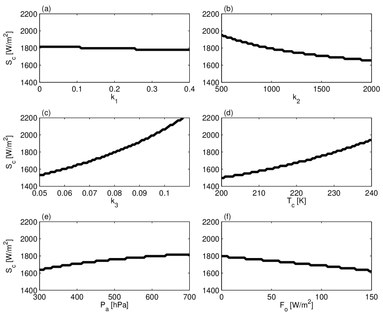
In Fig. 11, we show how $S_{c}$ changes as we vary $k_{1}$, $k_{2}$, $k_{3}$, $T_{c}$, $P_{a}$, and $F_{o}$, which are the most important independent parameters of the model. Here, $k_{1}$ represents the strength of adiabatic warming on the nightside surface due to large-scale dry descent (Eq. (9)); $k_{2}$ is a coefficient relating water vapor to the infrared opacity (Eq. (10)); $k_{3}$ is a constant that relates the strength of convection to the cloud fraction (Eq. (13)); $T_{c}$ is the cloud emission temperature; $P_{a}$ is the depth of convection; $F_{o}$ is the strength of ocean heat transport.

Changing $k_{1}$, $P_{a}$, and $F_{o}$ does not influence the value of $S_{c}$ very much (Fig. 11). In contrast, $k_{2}$, $k_{3}$, and $T_{c}$ strongly influence $S_{c}$. Increasing $k_{2}$ increases the optical thickness due to water vapor. Since there is more water vapor on the dayside, this preferentially decreases $OLR_{1}$, and therefore decreases $S_{c}$. Although $k_{2}$ is a necessary parameter in the two-column model, models with a more sophisticated radiative transfer scheme should agree on water vapor emissivity, and therefore the processes represented by $k_{2}$ are unlikely to be a major source of uncertainty in $S_{c}$.

The effects of $k_{3}$ and $T_{c}$ on $S_{c}$ are more likely to be relevant for future studies. These parameters represent cloud processes, which can differ significantly between complicated climate models. Increasing the cloud emission temperature ($T_{c}$) decreases the strength of cloud longwave forcing, increasing $OLR_{1}$ and therefore increasing $S_{c}$. Increasing $k_{3}$ causes an increase in the cloud fraction for a given convective heat flux, which increases both the cloud albedo and the cloud longwave forcing. Because the cloud albedo cooling effect is always stronger than the cloud greenhouse warming effect, water vapor amount and consequently atmospheric emissivity decrease. Since this primarily increases the $OLR$ on the dayside, increasing $k_{3}$ causes $S_{c}$ to increase. Cloud behavior will therefore be critical for determining the critical stellar flux ($S_{c}$), and a measurement of $S_{c}$ will help us distinguish between different cloud models.

Finally we note that other factors that we have not explicitly included in the two-column model, such as atmospheric CO₂, can influence the day-night emission contrast. For example, simulations in CAM3 show that increasing the CO₂ concentration strengthens the day-night thermal emission contrast because it weakens the nightside inversion and leads to a stronger water vapor feedback on the warmer dayside (not shown). This can change the critical stellar flux by $\approx$400 W m^-2 when the CO₂ concentration is increased from 0 to 0.1 bar, so that large uncertainties in the CO₂ of an observed planet would make it harder to fit a cloud model to the observed thermal emission contrast.

6. Conclusions

We constructed a low-order two-column model to simulate the climate of tidally locked terrestrial planets near the inner edge of the habitable zone of M-dwarf stars. This model incorporates the weak-temperature-gradient approximation to calculate horizontal atmospheric heat transport, the fixed anvil temperature hypothesis to calculate the cloud longwave effect, and a simple convective cloud scheme to calculate the cloud albedo. Our main findings are as follows:

(1) The relatively few parameters of the two-column model can be tuned to reproduce the basic behavior of a very complicated global climate model and respond faithfully to variations in both the stellar flux and ocean heat transport. This suggests that the physical processes built into the two-column model are the most important ones for determining the climate of tidally-locked terrestrial planets.

(2) The two-column model clearly illustrates the importance of dayside clouds and a nightside “radiator fin” for determining the climate of tidally locked planets. Dayside clouds increase the planetary albedo, which cools the planet and delays the onset of a runaway greenhouse. The radiator fin, primarily maintained by the dryness of the atmosphere and the temperature inversion on the nightside, allows the planet to easily lose energy to space through infrared thermal emission, which also cools the planet. Atmospheric dynamics are crucial for both of these effects, so they cannot be calculated by 1D radiative-convective models. This means that 1D radiative-convective models will tend to produce overly conservative estimates of the inner edge of the habitable zone.

(3) Observations of the day–night thermal emission contrast will be critical for deciphering the climate of tidally locked terrestrial planets. As the stellar flux increases, nightside emission increases faster than dayside emission, so that at a critical stellar flux there will be a reversal in the day–night thermal emission contrast, with higher emission from the nightside. Sensitivity experiments in the two-column model show that cloud variables are most likely to cause differences in the critical stellar flux between different models. This means that future observations of the day–night thermal emission contrast will be useful for distinguishing between cloud models.

References

- Abbot & Tziperman (2009) Abbot, D. S., & Tziperman, E. 2009, J. Atmos. Sci., 66, 519
- Clement & Seager (1999) Clement, A. C., & Seager, R. 1999, J. Clim., 12, 3384
- Collins et al. (2004) Collins, W. D., Basch, P. J., Boville, B. A., et al. 2004, Technical Note, Document NCAR-TN-464+STR (Boulder, CO: NCAR)
- Donohoe & Battisti (2011) Donohoe, A., & Battisti, D. S. 2011, J. Clim., 24, 4402
- Edson et al. (2011) Edson, A., Lee, S., Pollard, D., Bannon, P. R., & Kasting, J. F. 2011, Icarus, 212, 1
- Emanuel (1994) Emanuel, K. 1994, Atmospheric Convection (New York: Oxford University Press)
- Emanuel (2002) Emanuel, K. 2002, J. Geophys. Res., 107, 4077
- Farneti & Vallis (2013) Farneti, R., & Vallis, G. K. 2013, J. Clim., 26, 7151
- Goldblatt et al. (2013) Goldblatt, C., Robinson, T. D., Zahnle, K. J., & Crisp, D. 2013, Nature Geosci., 6, 661
- Hack et al. (2006) Hack, J. J., Caron, J. M., Yeager, S. G., et al. 2006, J. Clim., 19, 2199
- Hartmann & Larson (2002) Hartmann, D. L., & Larson, K. 2002, Geophys. Res. Lett., 29, 1951
- Hartmann & Michelsen (1993) Hartmann, D. L., & Michelsen, M. L. 1993, J. Clim., 6, 2049
- Heng & Vogt (2011) Heng, K, & Vogt, S. S. 2011, MNRAS, 415, 2145
- Houze & Betts (1981) Houze, R. A., & Betts, Jr A. K. 1981, Rev. Geophys., 19(4), 541
- Hu & Ding (2011) Hu, Y., & Ding, F. 2011, A&A, 526, A135
- Hu & Yang (2014) Hu, Y., & Yang, J. 2014, Proc. Natl. Acad. Sci. U.S.A., 111, 629
- Joshi (2003) Joshi, M. M. 2003, Astrobiology, 3, 415
- Joshi et al. (1997) Joshi, M. M., Haberle, R. M., & Reynolds, R. T. 1997, Icarus, 129, 450
- Kasting et al. (1993) Kasting, J. F., Whitmire, D. P., & Reynolds, R. T. 1993, Icarus, 101, 108
- Kitzmann et al. (2010) Kitzmann, D., Patzer, A. B. C., vonParis, P., et al. 2010, A&A, 511, A66
- Knutson et al. (2007) Knutson, H. A., Charbonneau, D., Allen, L. E., et al. 2007, Nature, 447, 183
- Kopparapu et al. (2013) Kopparapu, R. K., Ramirez, R., Kasting, J. F., et al. 2013, ApJ, 767, 131
- Kuang & Hartmann (2007) Kuang, Z., & Hartmann, D. L. 2007, J. Clim., 20, 2051
- Larson et al. (1999) Larson, K., Hartmann, D. L., & Klein, S. A. 1999, J. Clim., 12, 2359
- Leconte et al. (2013) Leconte, J., Forget, F., Charnay, B., et al. 2013, A&A, 554, A69
- Li et al. (2012) Li, Y., Yang, P., North, G. R., & Dessler A. 2012, J. Atmos. Sci., 69, 2317
- Merlis & Schneider (2010) Merlis, T. M., & Schneider, T. 2010, J. Adv. Model. Earth Syst., 2, 13
- Mills & Abbot (2013) Mills, S. M., & Abbot, D. S. 2013, ApJL, 774, L17
- Neale et al. (2010a) Neale, R. B., Richter, J. H., Conley, A. J., et al. 2010a, Technical Note, Document NCAR-TN-485+STR (Boulder, CO: NCAR)
- Neale et al. (2010b) Neale, R. B., Chen, C.-C., Gettelman, A., et al. 2010b, Technical Note, Document NCAR-TN-486+STR (Boulder, CO: NCAR)
- Perez-Becker & Showman (2013) Perez-Becker, D. & Showman, A. P. 2013, ApJ, 776, 134
- Pierrehumbert (1995) Pierrehumbert, R. T. 1995, J. Atmos. Sci., 52, 1784
- Pierrehumbert (2010) Pierrehumbert, R. T. 2010, Principles of Planetary Climate (Cambridge: Cambridge University Press)
- Pierrehumbert (2011) Pierrehumbert, R. T. 2011, ApJL, 726, L8
- Ramanathan & Collins (1991) Ramanathan, V., & Collins, W. 1991, Nature, 351, 27
- Ramanathan et al. (1989) Ramanathan, V., Cess, R. D., Harrison, E. F., et al. 1989, Science, 243, 57
- Raymond (1995) Raymond, D. J. 1995, J. Atmos. Sci., 55(22), 3945
- Shields et al. (2013) Shields, A. L., Meadows, V. S., Bitz, C. M., et al. 2013, Astrobiology, 13(8), 715
- Showman & Polvani (2011) Showman, A. P., & Polvani, L. M. 2011, ApJ, 738, 71
- Showman et al. (2013) Showman, A. P., Wordsworth, R. D., Merlis, T. M., & Kaspi, Y. 2013, in Comparative Climatology of Terrestrial Planets, eds. Mackwell, S. J., et al. (Tucson, AZ: University of Arizona Press), pp. 277-326.
- Slingo (1980) Slingo, J. M. 1980, Q. J. R. Meteorol. Soc., 106, 747
- Sobel et al. (2001) Sobel, A. H., Nilsson, J., & Polvani, L. M. 2001, J. Clim., 58, 3650
- Stone (1978) Stone, P. H. 1978, Dyn. Atmos. Oceans, 2, 123
- Tarter et al. (2007) Tarter, J. C., Backus, P. R., Mancinelli, R. L., et al. 2007, Astrobiology, 7, 30
- Wordsworth et al. (2010) Wordsworth, R. D., Forget, F., Selsis, F., et al. 2010, A&A, 522, A22
- Wordsworth et al. (2011) Wordsworth, R. D., Forget, F., Selsis, F., et al. 2011, ApJL, 73, L48
- Xu & Emanuel (1989) Xu, K., & Emanuel, K. A. 1989, Mon. Wea. Rev., 117, 1471
- Xu & Krueger (1991) Xu, K. M., & Krueger, S. K. 1991, Mon. Wea. Rev., 119(2), 342
- Yang et al. (2013) Yang, J., Cowan, N. B., & Abbot, D. S. 2013, ApJL, 771, L45
- Zelinka & Hartmann (2010) Zelinka, M. D., & Hartmann, D. L. 2010, J. Geophys. Res., 115, D16117, doi:10.1029/2010JD013817
- Zsom et al. (2012) Zsom, A., Kaltenegger, L., & Goldblatt, C. 2012, Icarus, 221, 603