Ground-state structures in Ising magnets on the Shastry-Sutherland lattice with long-range interactions and fractional magnetization plateaus in TmB₄

Abstract

A method for the study of the ground states of lattice-gas models or equivalent spin models with extended-range interactions is developed. It is shown that effect of longer-range interactions can be studied in terms of the solution of the ground-state problem for a model with short-range interactions. The method is applied to explain the emergence of fractional magnetization plateaus in TmB₄ that is regarded as a strong Ising magnet on the Shastry-Sutherland lattice.

I Introduction

Exact determination of the ground-state structures for complex lattice-gas models or equivalent spin models still remains an open problem despite considerable effort made for more than half a century bib1 ; bib2 . Many methods, both analytical and numerical, have been proposed bib3 ; bib4 ; bib5 ; bib6 , however, an universal effective algorithm has not been found as yet. We have elaborated a new method for the study of ground states for such models and successfully applied it to some interesting physical problems bib7 ; bib8 ; bib9 ; bib10 ; bib11 ; bib12 . In the present paper, we develop the method in order to show how to treat (at least partially) the effect of longer-range interactions in terms of the solution of the ground-state problem for a model with short-range interactions. We demonstrate this by considering a system of Ising spins on the Shastry-Sutherland (SS) lattice [see Fig. 1(a)] in the presence of an external magnetic field. The ground-state magnetic structures of this system are interesting because they are associated with the emergence of fractional magnetization plateaus in some rare-earth-metal tetraborides, particularly in TmB₄ regarded as a strong Ising magnet bib14 ; bib15 .

This compound consists of weakly coupled layers of magnetic ions Tm³⁺ arranged on a lattice that is topologically equivalent to the SS one. Experiments show that, in addition to a large 1/2-magnetization plateau, TmB₄ exhibits a sequence of narrow fractional magnetization plateaus at 1/6, 1/7, up to 1/12 of the saturation magnetization for temperatures below 4 K, with the magnetic field being normal to SS planes bib14 ; bib15 . In spite of considerable effort made to find the origin of these plateaus, only the 1/2-plateau has been reliably obtained in some theoretical works. Hence, the question remains open.

In Ref. bib12, , we found a complete solution of the ground-state problem for the Ising model on an extended SS lattice [Fig. 1(a)], i.e., with an interaction along the diagonals of “empty” squares (without SS bonds) in addition to the interactions along the edges of squares and the SS diagonals. In this model, the existence of a 1/2 plateau was proved. We have also shown that magnetic structures that can generate other fractional plateaus in TmB₄ are the ground-state ones at some boundaries of the full-dimensional ground-state regions of the four-dimensional parameter space of the model. At all the boundaries, a degeneracy exists. This degeneracy is at least twofold (in the case when only two nondegenerate phases exist at a boundary between these phases). But usually, the degeneracy is infinite and uncountable and often even macroscopic (i.e., leading to residual entropy).

Here, we determine the range of interactions which lift (at least partially) the degeneracy at three-dimensional boundaries of full (four)-dimensional ground-state regions as well as emerging full-dimensional (in the extended parameter space) phases that give rise to new magnetization plateaus. We do not consider all the three-dimensional boundaries but only those which can be associated with the emergence of fractional magnetization plateaus in rare-earth-metal tetraborides, particularly in TmB₄.

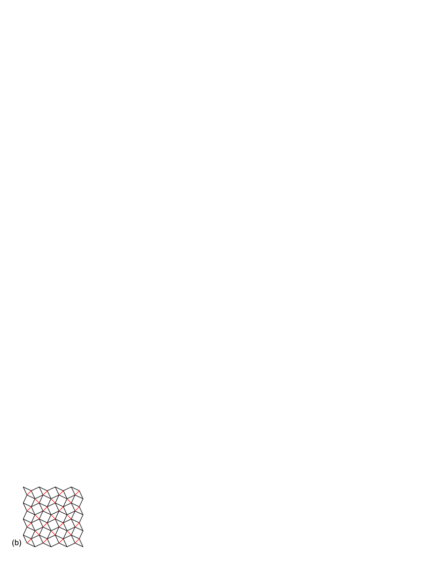
Figure 1: (Color online) (a) Extended Shastry-Sutherland lattice and (b) the lattice formed by magnetic Cu²⁺ ions in SrCu₂(BO₃)₂.

Although we consider a specific problem, the method developed here is general and may be applied to many other problems. The method is based on the notion of fractional contents of cluster configurations in the structures generated by these configurations and on some linear relations between these contents bib13 .

To enumerate pairwise interactions, we use the lattice shown in Fig. 1(b). The coordination circles for this lattice are shown in Fig. 2. We designate the $i$th-neighbor interaction on this lattice by $J_{i}$ except for the first- and second-neighbor interactions which are denoted by $\tilde{J}_{1}$ and $\tilde{J}_{2}$, respectively, in order to avoid the confusion with the notations introduced in Refs. bib11, and bib12, .

Figure 2: Top: Coordination circles and respective neighbors of the site depicted in black on the lattice that is topologically equivalent to the SS lattice. Bottom: Similar neighbors on the SS lattice. The sites contained in a “windmill” cluster (see Fig. 4) together with the central (black) site are depicted in yellow.

We construct structures on the lattice shown in Fig. 1(a), but name the clusters after their shapes on the lattice shown in Fig. 1(b). The clusters which we use here are depicted in Fig. 3. Similar cluster configurations are enumerated differently for different boundaries between full-dimensional regions.

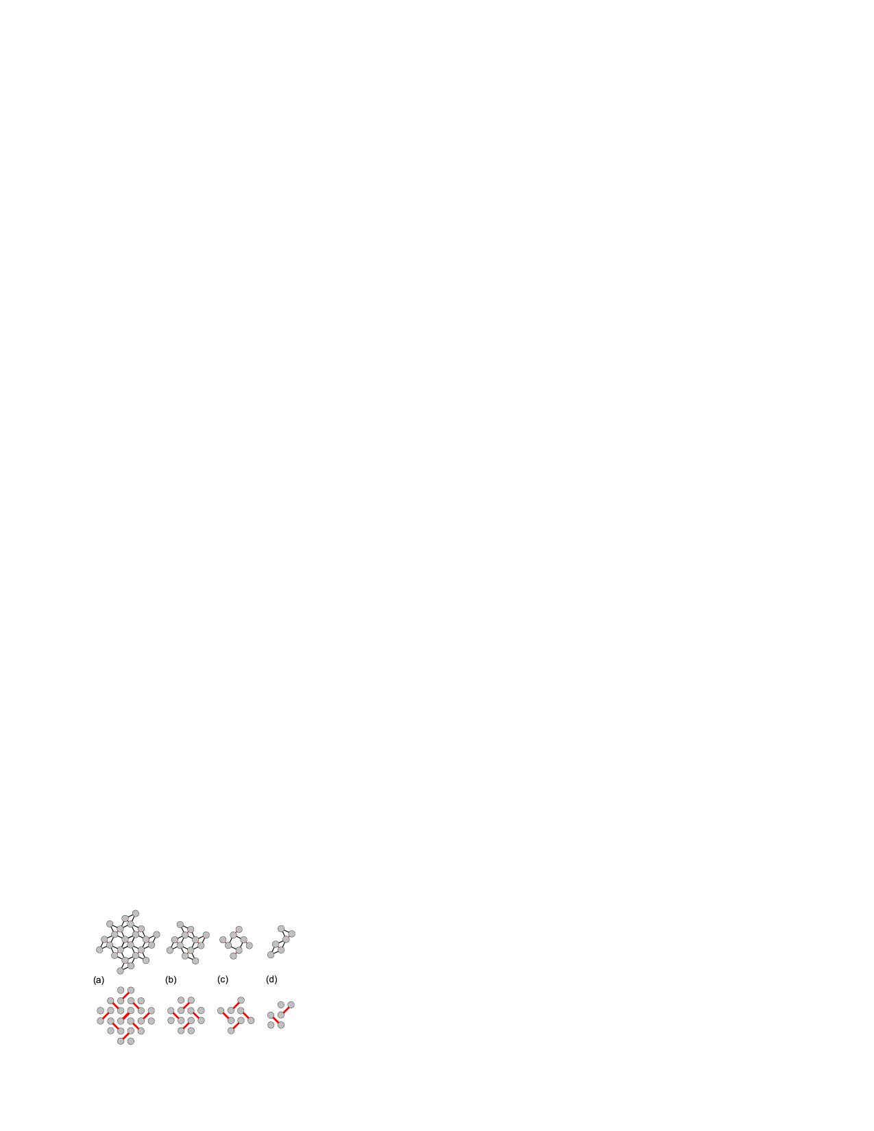
Figure 3: Clusters considered here: (a) “turtle”, (b) “windmill”, (c) “screw”, (d) “seahorse”. At the top and at the bottom, the clusters are depicted on the lattice shown in Fig. 1(b) and in Fig. 1(a), respectively.

II Full-dimensional ground-state structures emerging from the boundary between the Néel phase and the 1/3-plateau phase

In our previous papers, we have shown that, at the boundary between the Néel phase (phase 3) and the 1/3-plateau phase (phase 4) (see Fig. 4), the ground-state structures consist of the following configurations of the triangular cluster with SS bond as hypotenuse: , , and bib11 , or the equivalent set of square configurations, i.e., , , ; , and bib12 [herein solid and open circles denote spin up ($\sigma=+1$) and down ($\sigma=-1$), respectively]. This means that any triangular or square cluster in any ground-state structure at this boundary should have one of the listed configurations. It is easy to see that these structures represent antiferromagnetic stripes of various widths (domains of the Néel phase with even numbers of antiferromagnetic chains) separated by ferromagnetic chains [see Fig. 4(c)]. Longer-range interactions lift the degeneracy partially and lead to the emergence of new full-dimensional phases, that is, to the appearance of new fractional magnetization plateaus.

To study the effect of longer-range interactions, first, let us consider a windmill-shaped cluster. Its configurations generating all the structures at the boundary between phases 3 and 4 are shown in Fig. 5. It means that, in any ground-state structure at this boundary, any cluster of this type on the lattice has one of these configurations (or chiral ones). The structure shown in Fig. 6 is similar to that in Fig. 4(c) but with the number of the “windmill” configuration indicated in the center of each “empty” square.

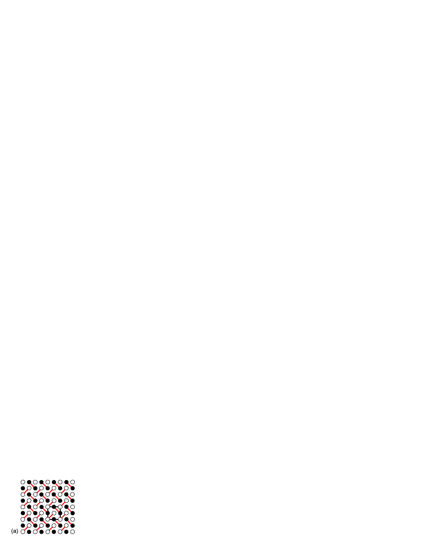
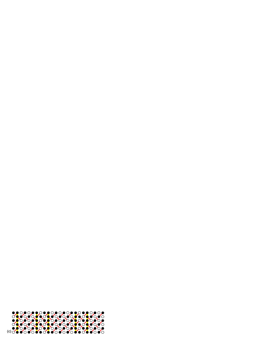
Figure 4: (a) Néel structure, (b) 1/3-plateau structure, and (c) a general disordered structure at the boundary of the relative phases (the yellow background indicates ferromagnetic chains).

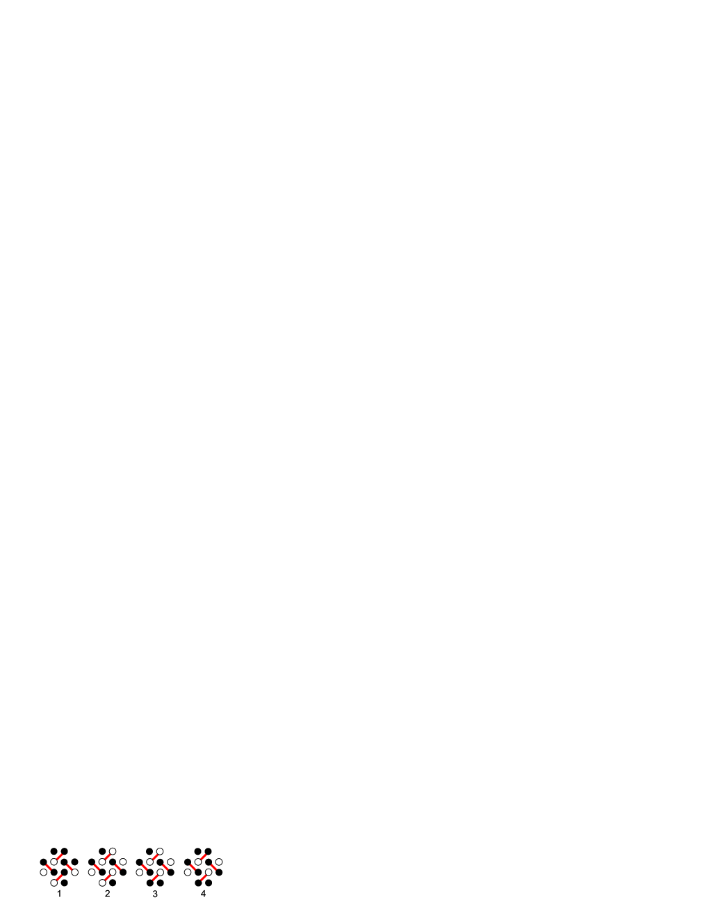
Figure 5: Configurations of the “windmill” cluster for the structures at the boundary between the Néel phase and the 1/3-plateau phase.

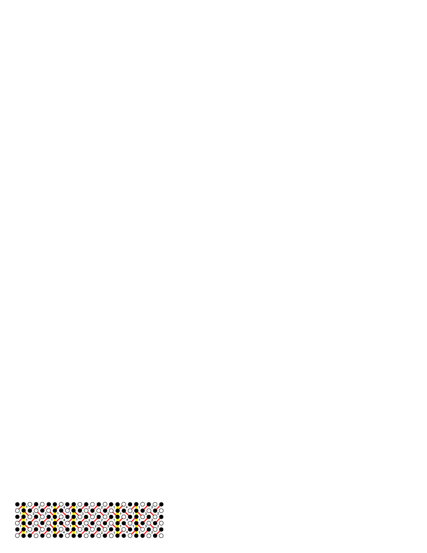
Figure 6: The similar structure as in Fig. 4(c), but with the number of the “windmill” configuration indicated in the center of each “empty” square.

Figure 7: A subcluster of the “windmill” cluster and its two nonequivalent positions in the cluster: central and lateral (enveloped by an ellipse).

We refer to the relative quantity of a configuration of a cluster in a structure as a fractional content of the configuration in the structure. Let $k_{1}$, $k_{2}$, $k_{3}$, and $k_{4}$ be the fractional contents of the configurations shown in Fig. 5 in the structures at the boundary between phases 3 and 4. In addition to the trivial relation between $k_{i}$ (the normalization condition),

$$k_{1}+k_{2}+k_{3}+k_{4}=1,$$ (1)

there is one more linear relation between these quantities (see bib13 ). To find it, let us consider a subcluster of the “windmill” cluster that has at least two nonequivalent positions in this cluster. Let it be the two-site subcluster shown in Fig. 7. It can occupy even four nonequivalent positions in the “windmill” cluster. Consider two of these: the central one (position 1) and the lateral one (position 2, enveloped by an ellipse in Fig. 7). In each position, the subcluster enters only one “windmill” cluster on the lattice: $c_{1}=c_{2}=1$. Let us consider the “two spins up” configuration of the subcluster and calculate the number of such configurations in each position for each configuration of the cluster: $n_{11}=2$, $n_{12}=0$, $n_{13}=0$, $n_{14}=0$, $n_{21}=1$, $n_{22}=0$, $n_{23}=1$, and $n_{24}=2$. Using the general relation

$$\sum_{l}\frac{k_{l}n_{1l}}{c_{1}}=\sum_{l}\frac{k_{l}n_{2l}}{c_{2}},$$ (2)

where $l$ is the number of the cluster configuration, we have

$$k_{1}-k_{3}-2k_{4}=0.$$ (3)

Other configurations of the subcluster or other subclusters yield the same relation. Hence, two of the four quantities $k_{1}$, $k_{2}$, $k_{3}$, and $k_{4}$ are independent, for instance, $k_{1}$ and $k_{2}$, and the other two can be linearly expressed in terms of these, i.e.,

$$k_{3}=-3k_{1}-2k_{2}+2,~{}~{}k_{4}=2k_{1}+k_{2}-1.$$ (4)

Bearing in mind that each site on the lattice belongs to six “windmill” clusters, we can find the magnetization per site for each structure generated by the set of cluster configurations under consideration, i.e.,

$$m=\frac{1}{6}(2k_{1}+k_{3}+2k_{4})=\frac{k_{1}}{2}.$$ (5)

Moreover, the magnetization per site is given by the relative number of ferromagnetic chains in the structure. Hence, this number is equal to $\frac{k_{1}}{2}$. In order $k_{2}$ to be maximum (minimum) for fixed $k_{1}$ (that is, for fixed number of ferromagnetic chains), the number of narrowest stripes (and hence, of configurations 4) should be maximum (minimum). This is clear from Fig. 6. Thus the region of variation for the quantities $k_{1}$ and $k_{2}$ is the triangle $ABC$ shown in Fig. 8. The vertex with the coordinates $k_{1}=0$, $k_{2}=1$ ($k_{3}=k_{4}=0$) corresponds to the Néel structure, and the vertex $k_{1}=2/3$, $k_{2}=0$ ($k_{3}=0$, $k_{4}=1/3$) corresponds to the 1/3-plateau structure. The vertex with the coordinates $k_{1}=2/5$, $k_{2}=1/5$ ($k_{3}=2/5$, $k_{4}=0$) corresponds to the only structure shown in Fig. 9.

Figure 8: Region of variation for the quantities $k_{1}$ and $k_{2}$. Vertexes $B(0,~{}1)$, $A(2/3,~{}0)$, and $C(2/5,~{}1/5)$ of the triangle $ABC$ correspond to the Néel structure, the 1/3-plateau structure, and the 1/5-plateau structure, respectively.

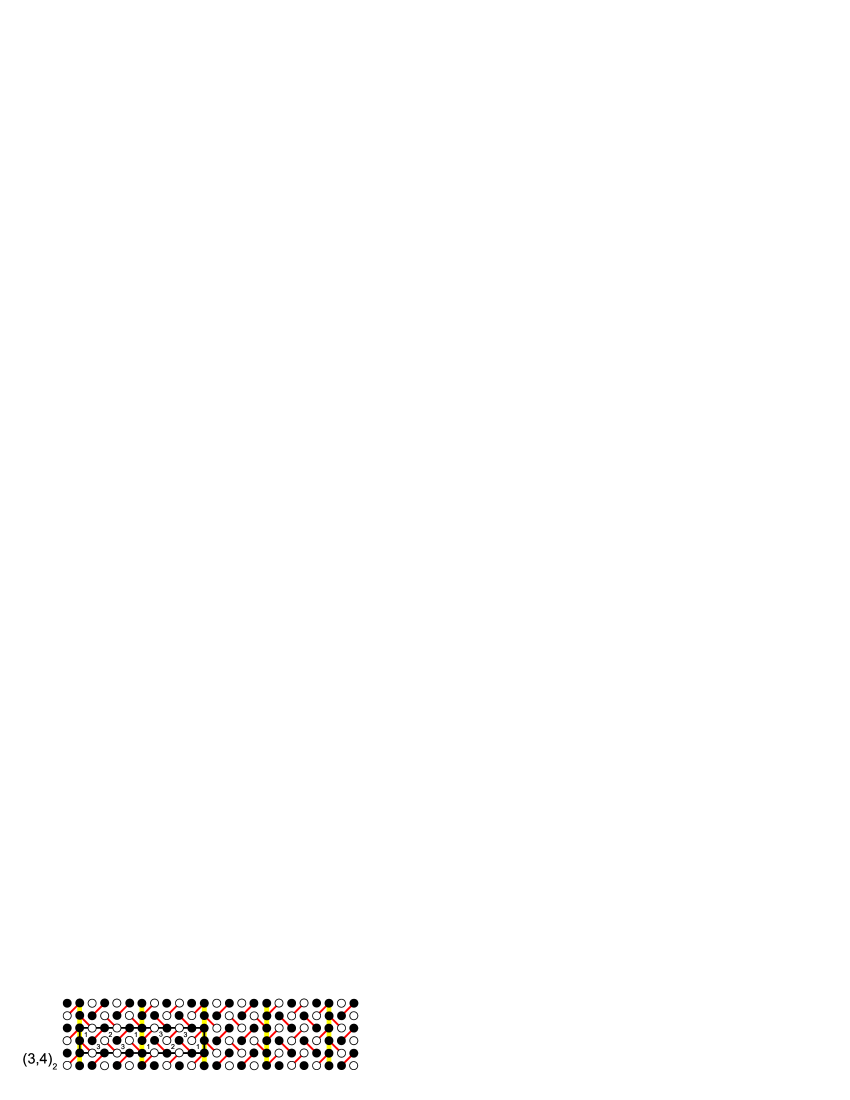
Figure 9: 1/5-plateau structure that emerges from the boundary between phases 3 and 4, if the interaction range reaches the seventh neighbors ($k_{1}=k_{3}=2/5$, $k_{2}=1/5$).

The fact that the region of variation for the quantities $k_{1}$ and $k_{2}$ is the triangle $ABC$, can be proved in other way, using relations (4). From the first of these we have the inequality

$$3k_{1}+2k_{2}-2=-k_{3}\leqslant 0,$$ (6)

which, being regarded as an equation, represents an equation of the straight line $AB$ ($k_{3}=0$). The second relation

$$2k_{1}+k_{2}-1=k_{4}$$ (7)

represents an equation of the straight line $BC$ for which $k_{4}=0$. For $k_{4}=0$, however, the minimum value of $k_{2}$ is equal to 1/5 rather than 0. This follows from the relation

$$3k_{1}+4k_{2}-2=2k_{2}-k_{3}\geqslant 0$$ (8)

and the inequality $2k_{2}\geqslant k_{3}$. Thus, we obtain the point $C(2/5,1/5)$ that corresponds to the structure shown in Fig. 9.

If all the interactions (pairwise as well as many-spin) occur within the “windmill” cluster, then the energy of a ground-state structure is a linear function of $k_{1}$ and $k_{2}$, and therefore (for fixed values of interactions and external field) it can reach the minimum value only at the boundary of the triangle shown in Fig. 8. Therefore, only the vertexes of the triangle correspond to the full-dimensional structures. Hence, the interactions within the “windmill” cluster can generate only one full-dimensional structure from the boundary between the Néel phase and the 1/3-plateau phase. This structure is shown in Fig. 9; it gives rise to the plateau with the magnetization 1/5. To determine the range of interactions which can generate this structure, let us find the contribution of various pairwise interactions (within the “windmill” cluster) into the energy density (i.e., energy per site). We have

$$e_{1}=\frac{1}{4}(-k_{1}+2k_{2}+k_{3})\tilde{J}_{1}=(-k_{1}+\frac{1}{2})\tilde{J}_{1},$$

$$e_{2}=-\frac{1}{2}(k_{1}+4k_{2}+3k_{3}+2k_{4})\tilde{J}_{2}=(2k_{1}-2)\tilde{J}_{2},$$

$$e_{3}=(k_{2}+k_{3}+k_{4})J_{3}=(-k_{1}+1)J_{3},$$

$$e_{4}=(k_{1}-2k_{2}-k_{3})J_{4}=(4k_{1}-2)J_{4},$$

$$e_{5}=(k_{1}+2k_{2}+k_{3})J_{5}=(-2k_{1}+2)J_{5},$$

$$e_{6}=\frac{1}{2}J_{6},$$

$$e_{7}=(-k_{1}+k_{2}+k_{4})J_{7}=(k_{1}+2k_{2}-1)J_{7},$$

$$e_{8}=-2(k_{2}+k_{3}+k_{4})J_{8}=(2k_{1}-2)J_{8},$$

$$e_{9a}=\frac{1}{2}(-k_{1}+2k_{2}+k_{3})J_{9}=(-2k_{1}+1)J_{9},$$

$$e_{11}=(k_{1}-2k_{2}-k_{3})J_{11}=(4k_{1}-2)J_{11},$$

$$e_{16}=(k_{2}+k_{3}+k_{4})J_{16}=(-k_{1}+1)J_{16}.$$ (9)

Since only a half of the number of ninth neighbors enter the “windmill” cluster (see Fig. 2), we denote their contribution to the energy density by $e_{9a}$.

Thus, contributions $e_{i}$ to the energy density of all the pairwise interactions within the “windmill” cluster except for the seventh neighbors depend on the magnetization of the structure only, that is, on $k_{1}$. However, $e_{7}$ depends also on $k_{2}$. This means that only the pairwise interaction of the seventh neighbors or many-spin interactions which include the seventh neighbors can lift the degeneracy at the boundary between the Néel phase and the 1/3-plateau phase giving rise to a new full-dimensional phase. This is the phase $(3,4)_{2}$ (see Ref. bib11, about the notations) with the magnetization 1/5 (Fig 9).

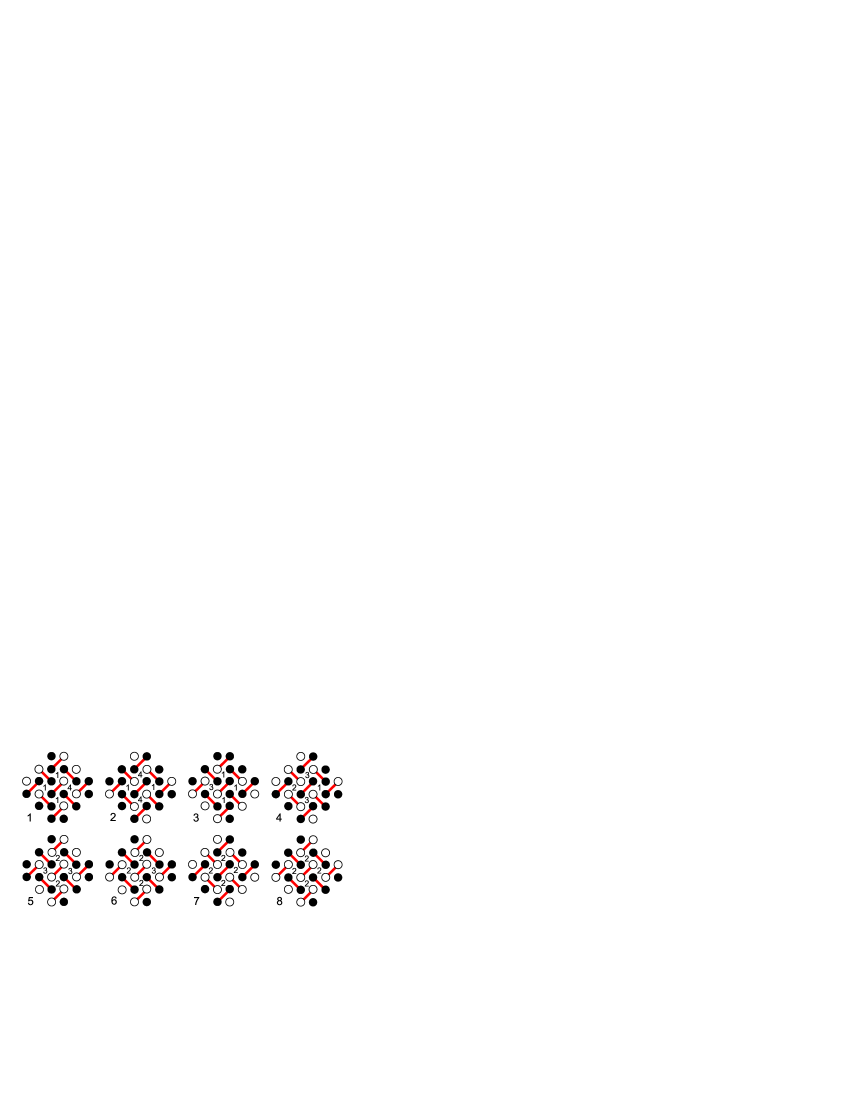
Figure 10: Configurations of the “turtle” cluster which generate all the ground-state structures at the boundary between the Néel phase and the 1/3-plateau phase. Each “empty” square contains the number of the “windmill” configuration with the center in this square (see Fig. 5).

In order to take into account interactions beyond the “windmill” cluster, we consider a bigger cluster whose shape resembles a turtle. The ground-state configurations of this cluster for the boundary between the Néel phase and the 1/3-plateau phase are shown in Fig. 10.

Figure 11: Maximum subcluster which can occupy two nonequivalent positions in the “turtle” cluster.

Considering the configurations of the maximum subcluster among those which can occupy two nonequivalent positions in the “turtle” cluster (Fig. 11), we find the relations between the fractional contents $l_{i}$ of these configurations in the ground-state structures to be given by

$$l_{1}-2l_{2}=0,$$

$$l_{3}-l_{4}=0,$$

$$l_{4}-2l_{5}-l_{6}=0,$$

$$l_{6}-2l_{7}+2l_{8}=0.$$ (10)

Thus, only three of the eight normalized quantities $l_{i}$ are independent. Let it be $l_{1}$, $l_{3}$, and $l_{5}$. The rest of the quantities $l_{i}$ can be expressed in terms of these, i.e.,

$$l_{2}=\frac{1}{2}l_{1},$$

$$l_{4}=l_{3},$$

$$l_{6}=l_{3}-2l_{5},$$

$$l_{7}=-\frac{3}{4}l_{1}-\frac{5}{4}l_{3}+\frac{1}{2},$$

$$l_{8}=-\frac{3}{4}l_{1}-\frac{7}{4}l_{3}+l_{5}+\frac{1}{2}.$$ (11)

The quantities $k_{i}$ can be expressed in terms of $l_{1}$ and $l_{3}$ as well. To do this we just have to calculate the number of configurations of the “windmill” subcluster in the configurations of the “turtle” cluster. Thus we have

$$k_{1}=l_{1}+l_{3},~{}~{}k_{2}=-\frac{3}{2}l_{1}-2l_{3}+1,$$

$$k_{3}=l_{3},~{}~{}k_{4}=\frac{1}{2}l_{1}.$$ (12)

As follows from these relations,

$$l_{1}=4k_{1}+2k_{2}-2,~{}~{}l_{3}=-3k_{1}-2k_{2}+2.$$ (13)

Hence, in addition to the two independent quantities $k_{1}$ and $k_{2}$, we have one more independent quantity, $l_{5}$. The quantities $k_{1}$ and $k_{2}$ determine the number of stripes with two antiferromagnetic chains (we denote this stripe by $s_{1}$), and $l_{5}$ determines the number of stripes with four antiferromagnetic chains (we denote this stripe by $s_{2}$). The region of variation for $k_{1}$, $k_{2}$, and $l_{5}$ is shown in Fig. 12. This is the pyramid $ABCD$. The points of the face $BCD$ correspond to the structures without stripes $s_{1}$. The structures which correspond to the edge $BD$ do not contain the stripes $s_{1}$ and $s_{2}$; in the structures corresponding to the edge $BC$, the number of stripes $s_{2}$ is maximum. The face $ABC$ corresponds to the structures with maximum numbers of stripes $s_{2}$. The projection of this pyramid on the $(k_{1},k_{2})$ plane is similar to the triangle shown in Fig. 8.

Figure 12: Region of variation for the quantities $k_{1}$, $k_{2}$, and $l_{5}$. Each vertex corresponds to a full-dimensional structure.

Let us prove rigorously that the tetrahedron $ABCD$ is indeed the region of variation for the quantities $k_{1}$, $k_{2}$, and $l_{5}$. It is determined by four inequalities given by

$$ABC:3k_{1}+2k_{2}-2+2l_{5}\leqslant 0,$$

$$ACD:9k_{1}+8k_{2}-6+4l_{5}\geqslant 0,$$

$$BCD:2k_{1}+k_{2}-1\geqslant 0,$$

$$ABD:l_{5}\geqslant 0.$$ (14)

The first one follows from relations $l_{3}-2l_{5}=l_{6}$ and $l_{3}=-3k_{1}-2k_{2}+2$ [the third relation from (9) and the second one from (12)]. Hence, for the face $ABC$, the value of $l_{6}$ is equal to zero. The second inequality follows from the last relation of (10) and relations (12). For the face $ACD$, the value of $l_{8}$ is equal to zero. The inequality for the face $BCD$ is the same as for the straight line $BC$ for which $k_{4}=0$ (i.e., the structures on this face have no narrow stripes $s_{1}$).

Figure 13: Structure with magnetization 1/7 that emerges from the boundary between phases 3 and 4 if the range of interaction reaches the 21th neighbors (five square lattice constants). For this structure $k_{1}=\frac{2}{7}$, $k_{2}=\frac{3}{7}$, and $l_{5}=0$.

Figure 14: Structure with magnetization 1/4 that emerges from the boundary between phases 3 and 4 if the range of interaction reaches the 32th neighbors (six square lattice constants). For this structure $k_{1}=\frac{1}{2}$, $k_{2}=\frac{1}{8}$, and $l_{5}=\frac{1}{8}$.

Figure 15: Pairwise interactions on the SS lattice which can be taken into account by considering the “turtle” cluster (see Fig. 4). The corresponding neighbors of the central site (the black circle) are depicted in yellow.

Thus, interactions within the “turtle” cluster which are absent in the “windmill” cluster can generate only one additional full-dimensional structure, the structure with $k_{1}=2/7$, $k_{2}=3/7$, and $l_{5}=0$. It is shown in Fig. 13. The magnetization of this structure is equal to 1/7.

To determinate the range of interactions which can give rise to this structure, let us find the contribution to the energy density of various pairwise interactions within the “turtle” cluster which (except for 9th, 11th, and 16th neighbors) are absent in the “windmill” cluster (see Fig. 15). It should be noted that only two sites belong to one “turtle” cluster on the lattice. Thus, we have

$$e_{9}=2(-l_{1}+l_{2}-l_{3}+l_{4}+l_{5}+l_{6}+l_{7}+l_{8})J_{9}$$

$$~{}~{}~{}~{}=(-4k_{1}+2)J_{9},$$

$$e_{10}=(l_{2}+l_{5}+l_{6}+l_{7}+l_{8})J_{10}$$

$$~{}~{}~{}~{}~{}=(-l_{1}-2l_{3}+1)J_{10}=(2k_{1}+2k_{2}-1)J_{10},$$

$$e_{11}=2(l_{2}-l_{5}-l_{6}-l_{7}-l_{8})J_{11}=(4k_{1}-2)J_{11},$$

$$e_{12}=2(l_{1}+l_{2}+l_{3}-l_{5}-l_{6}-l_{7}-l_{8})J_{12}$$

$$~{}~{}~{}~{}~{}=(6k_{1}-2)J_{12},$$

$$e_{13}=(-l_{1}+l_{2}-l_{3}+l_{5}+l_{6}+l_{7}+l_{8})J_{13}$$

$$~{}~{}~{}~{}~{}=(-2k_{1}+1)J_{13},$$

$$e_{14}=\frac{1}{2}(-l_{1}+l_{2}-l_{3}-l_{4}+l_{5}+l_{6}+l_{7}+l_{8})J_{14}$$

$$~{}~{}~{}~{}~{}=(-l_{1}-2l_{3}+\frac{1}{2})J_{14}=(2k_{1}+2k_{2}-\frac{3}{2})J_{14},$$

$$e_{15}=(-2l_{2}+l_{3}-l_{6}-2l_{7}-2l_{8})J_{15}$$

$$~{}~{}~{}~{}~{}=(2l_{1}+6l_{3}-2)J_{15}=(-10k_{1}-8k_{2}+6)J_{15},$$

$$e_{16}=(l_{2}+l_{4}+l_{5}+l_{6}+l_{7}+l_{8})J_{16}$$

$$~{}~{}~{}~{}~{}=(-k_{1}+1)J_{16},$$

$$e_{17}=(l_{1}+l_{3}-l_{4}-2l_{5}-2l_{6}-2l_{7}-2l_{8})J_{17}$$

$$~{}~{}~{}~{}~{}=(4k_{1}-2)J_{17},$$

$$e_{18}=(l_{1}+l_{4}+l_{6}+2l_{7}+2l_{8})J_{18}$$

$$~{}~{}~{}~{}~{}=(-2l_{1}-4l_{3}+2)J_{18}=(4k_{1}+4k_{2}-2)J_{18},$$

$$e_{20a}=\frac{1}{4}(-4l_{1}-6l_{3}+4l_{5}+6l_{6}+8l_{7}+8l_{8})J_{20}$$

$$~{}~{}~{}~{}~{}=(-4l_{1}-6l_{3}+2)J_{20}=(2k_{1}+4k_{2}-2)J_{20},$$

$$e_{21}=(l_{2}-l_{3}+l_{5}+l_{7}+l_{8})J_{21}$$

$$~{}~{}~{}~{}~{}=(-l_{1}-4l_{3}+2l_{5}+1)J_{21}$$

$$~{}~{}~{}~{}~{}=(8k_{1}+6k_{2}+2l_{5}-5)J_{21},$$

$$e_{22}=(l_{1}+l_{3}-l_{4}-2l_{5}-2l_{6}-2l_{7}-2l_{8})J_{22}$$

$$~{}~{}~{}~{}~{}=(4l_{1}+4l_{3}-2)J_{22}=(4k_{1}-2)J_{22},$$

$$e_{25}=\frac{1}{6}(-l_{1}-l_{2}-l_{3}+l_{4}+3l_{5}+3l_{6}+3l_{7}+3l_{8})J_{25}$$

$$~{}~{}~{}~{}~{}=\frac{1}{6}(-6l_{1}-6l_{3}+3)J_{25}=(-k_{1}+\frac{1}{2})J_{25},$$

$$e_{26}=\frac{1}{2}(-4l_{2}+2l_{3}-2l_{6}-4l_{7}-4l_{8})J_{26}$$

$$~{}~{}~{}~{}~{}=(2l_{1}+6l_{3}-2)J_{26}=(-10k_{1}-8k_{2}+6)J_{26},$$

$$e_{34}=(l_{2}+l_{5}+l_{6}+l_{7}+l_{8})J_{34}$$

$$~{}~{}~{}~{}~{}=(-l_{1}-2l_{3}+1)J_{34}=(2k_{1}+2k_{2}-1)J_{34}.$$ (15)

The “turtle” cluster contains only a half of the 20th-neighbor pairs (see Fig. 15); therefore, we denote their contribution to the energy density by $e_{20a}$.

We thus see that contributions $e_{i}$ to the energy density of all the pairwise interactions within the “turtle” cluster except for the 21th neighbors, depend on $k_{1}$ and $k_{2}$. However, the contribution of the 21th neighbors depends not only on these quantities but also on $l_{5}$. Hence, only the pairwise interaction of 21th neighbors or many-spin interactions, which includes 21th neighbors, can give rise to a full-dimensional structure that cannot be produced by any interaction within the “windmill” cluster. As we have already shown, this is the 1/7-plateau structure (Fig. 13).

Having directly calculated the contributions of various pairwise interactions, that do not enter the “turtle” cluster, to the energy density (up to the 43th neighbors) for 1/3-, 1/4-, 1/5-, and 1/7-plateau structures as well as for the Néel structure, we find that

$$e_{19}=(k_{1}+2k_{2}-1)J_{19}$$

$$e_{20}=2e_{20a}=2(2k_{1}+4k_{2}-2)J_{20},$$

$$e_{23}=(-8k_{1}-8k_{2}+6)J_{23},$$

$$e_{24}=(9k_{1}+6k_{2}+2l_{5}-5)J_{24},$$

$$e_{27}=(11k_{1}+8k_{2}+2l_{5}-7)J_{27},$$

$$e_{28}=(-4k_{1}-4k_{2}+3)J_{28},$$

$$e_{29}=(6k_{1}-2)J_{29},$$

$$e_{30}=(k_{1}+2k_{2}-1)J_{30},$$

$$e_{31}=(-10k_{1}-8k_{2}+6)J_{31},$$

$$e_{32}=(-16k_{1}-12k_{2}-8l_{5}-\frac{1}{2}q+10)J_{32},$$

$$e_{33}=(8k_{1}+8k_{2}-6)J_{33},$$

$$e_{35}=(8k_{1}+6k_{2}+2l_{5}-5)J_{35},$$

$$e_{36}=(18k_{1}+12k_{2}+4l_{5}-10)J_{36},$$

$$e_{37}=(4k_{1}+4k_{2}-3)J_{37},$$

$$e_{38}=(-22k_{1}-16k_{2}+14)J_{38},$$

$$e_{39}=(-14k_{1}-12k_{2}-8l_{5}-\frac{1}{2}q+10)J_{39},$$

$$e_{40}=(32k_{1}+24k_{2}+8l_{5}-20)J_{40},$$

$$e_{41}=(9k_{1}+6k_{2}+2l_{5}-\frac{11}{2})J_{41},$$

$$e_{42}=(k_{1}+2k_{2}-1)J_{42},$$

$$e_{43}=(-10k_{1}-8k_{2}+6)J_{43}.$$ (16)

To prove these relations rigorously, one should consider clusters larger than the “turtle” cluster but we do not do it here.

The contributions of the 32th-neighbor interaction to the energy density for the 1/3-, 1/4-, 1/5-, and 1/7-plateau structures as well as for the Néel structure are given by

$$e_{32,N}=-2J_{32},~{}~{}e_{32,1/3}=-\frac{2}{3}J_{32},~{}~{}e_{32,1/4}=-J_{32},$$

$$e_{32,1/5}=-\frac{2}{5}J_{32},~{}~{}e_{32,1/7}=\frac{2}{7}J_{32}.$$ (17)

The quantity $e_{32}$ (as well as $e_{39}$) cannot be written in the form $ak_{1}+bk_{2}+cl_{5}+d$, as one can do for all the interactions up to the 31th neighbors and also for 33-38th and 40-43th neighbors. In addition to $k_{1}$, $k_{2}$, and $l_{5}$ a new quantity, $q$, should be introduced. Thus, the 32th neighbor interaction (as well as the 39th neighbors interaction) gives rise to a new full-dimensional phase. This phase just corresponds to the 1/4-plateau structure $(3,4)_{1,2}$ (Fig. 14).

The contributions of the 44th-neighbor interaction to the energy density for the 1/3-, 1/4-, 1/5-, and 1/7-plateau structures as well as for the Néel structure are given by

$$e_{44,N}=J_{44},~{}~{}~{}~{}~{}~{}~{}~{}e_{44,1/3}=-\frac{1}{3}J_{44},$$

$$e_{44,1/4}=\frac{1}{2}J_{44},~{}~{}~{}~{}e_{44,1/5}=\frac{1}{5}J_{44},$$

$$e_{44,1/7}=-\frac{1}{7}J_{44},~{}~{}e_{44,1/9}=-\frac{1}{9}J_{44}.$$ (18)

The 44th-neighbor interaction again gives rise to a new full-dimensional phase, $(3,4)_{4}$, that is the 1/9-plateau phase.

Now we can conclude that new full-dimensional phases can emerge from the boundary between phases 3 and 4 when new pairs of chains begin to interact. Thus, the interactions of chains at the distances of three and five square lattice constants (the seventh and 21th neighbors) can give rise to the 1/5-, and 1/7-plateau phases, respectively. The $1/n$-plateau phase, where $n$ is odd (even) number, can emerge only provided the chains at the distance of $n-2$ ($2n-2$) square lattice constants interact.

New plateaus can emerge in the following succession with increasing interaction range: 1/5 plateau (the 7th neighbor interaction, i.e, the interaction of chains at the distance of three square lattice constants); 1/7 plateau (21th neighbors, 5 constants); 1/4 plateau (32th neighbors, 6 constants); 1/9 plateau (44th neighbors, 7 constants); 1/5 plateau (8 constants); 1/11 and 3/11 plateaus (9 constants); 1/6 plateau (10 constants); 1/13 and 3/13 plateaus (11 constants); … The 1/5 plateau which follows the 1/9 plateau corresponds to a structure that differs from the 1/5-plateau structure shown in Fig. 9.

What sequences of phases (i.e., sequences of plateaus) are possible with the field increase, if the interactions do not overstep, for instance, the bounds of the “turtle” cluster? There are four paths from the vertex $B$ to the vertex $A$ of the tetrahedron $ABCD$ along its edges: $BA$, $BCA$, $BDA$, and $BDCA$. These paths correspond to the sequences of plateaus 0–1/3, 0–1/5–1/3, 0–1/7–1/3, and 0–1/5–1/7–1/3. It depends on the signs and values of interactions, which of these sequences is realized.

If the interactions up to the 44th neighbors are involved into consideration, then only the 1/9-, 1/7-, 1/5-, and 1/4-plateau phases can emerge at the boundary between the Néel phase and the 1/3-plateau phase. It depends on the interaction constants $J_{i}$, which of these phases “survive.” The interaction constants are determined by the exchange interaction between the nearest neighbors and by the Ruderman-Kittel-Kasuya-Yosida (RKKY) interaction.

The RKKY interaction in two dimensions reads bib22

$$H_{RKKY}=A^{2}\frac{m(k_{F})^{2}}{8\pi}[J_{0}(k_{F}R_{ij})Y_{0}(k_{F}R_{ij})$$

$$~{}~{}~{}~{}~{}~{}~{}~{}~{}~{}~{}+J_{1}(k_{F}R_{ij})Y_{1}(k_{F}R_{ij})]\sigma_{i}\sigma_{j},$$ (19)

where $J_{0}$ and $J_{1}$ are the Bessel functions of the first kind of the zero and first orders, respectively, $Y_{0}$ and $Y_{1}$ are the Bessel functions of the second kind of the zero and first orders, respectively, $k_{F}$ is the Fermi level, $R_{ij}$ is the distance between the sites $i$ and $j$, $\sigma_{i}$ and $\sigma_{j}$ are the values of Ising spins at the sites $i$ and $j$, $m$ is an effective mass of conduction electrons, and $A$ is the exchange coupling constant.

It depends on the value of $k_{F}$, which of the 1/9-, 1/7-,
1/5-, and 1/4-plateau structures become full-dimensional, with the value of $A$ influencing only the widths of the plateaus. In TmB₄ and ErB₄, magnetic atoms of each layer are arranged in the Archimedean lattice $3^{2}.4.3.4$ (see Fig. 16) which is topologically equivalent to the SS lattice. For these compounds, $\tilde{J}_{1}=\tilde{J}_{2}$.

If, for instance, the nearest-neighbor interaction is antiferromagnetic and equal to 1 ($\tilde{J}_{1}=\tilde{J}_{2}=1$), and the rest of $J_{i}$ ($i$ = 3–44) are determined by $k_{F}=4.14/a$, where $a$ is the side of a square or a triangle on the Archimedean lattice, then, among all the structures at the boundary between phases 3 and 4, only the 1/9- and 1/7-plateau structures become full-dimensional. Such plateaus are observed in TmB₄, though in Ref. bib14, slightly different structures are presented for these plateaus.

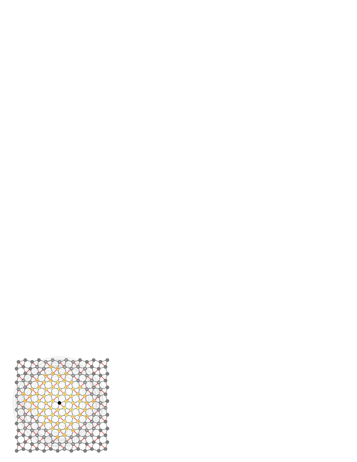
Figure 16: Coordination circles and respective neighbors of the site depicted in black on the Archimedean lattice $3^{2}.4.3.4$ that is topologically equivalent to the SS lattice. The sites are enumerated in the same manner as in Fig. 15. The sites which enter a “turtle” cluster (see Fig. 4) together with the central (black) site are depicted in yellow.

III Full-dimensional ground-state structures emerging from the boundary between the 1/3-plateau and 1/2-plateau phases

In a manner similar to the previous section, let us find the ground-state structures that can emerge from the boundary between the 1/3-plateau phase (phase 4) and the 1/2-plateau phase (phase 6) when the interaction range increases. The ground-state structures at this boundary consist of the square configurations , , , ; , and bib13 . We consider the configurations of the “windmill” cluster which generate all the ground-state structures at the boundary between phases 4 and 6. These are shown in Fig. 17. Configurations 1-3 and 12-21 generate the structures of phase 6 (that is disordered itself), and configurations 4 and 5 give rise to phase 4; configurations 6-11 are additional ones at the boundary between phases 4 and 6.

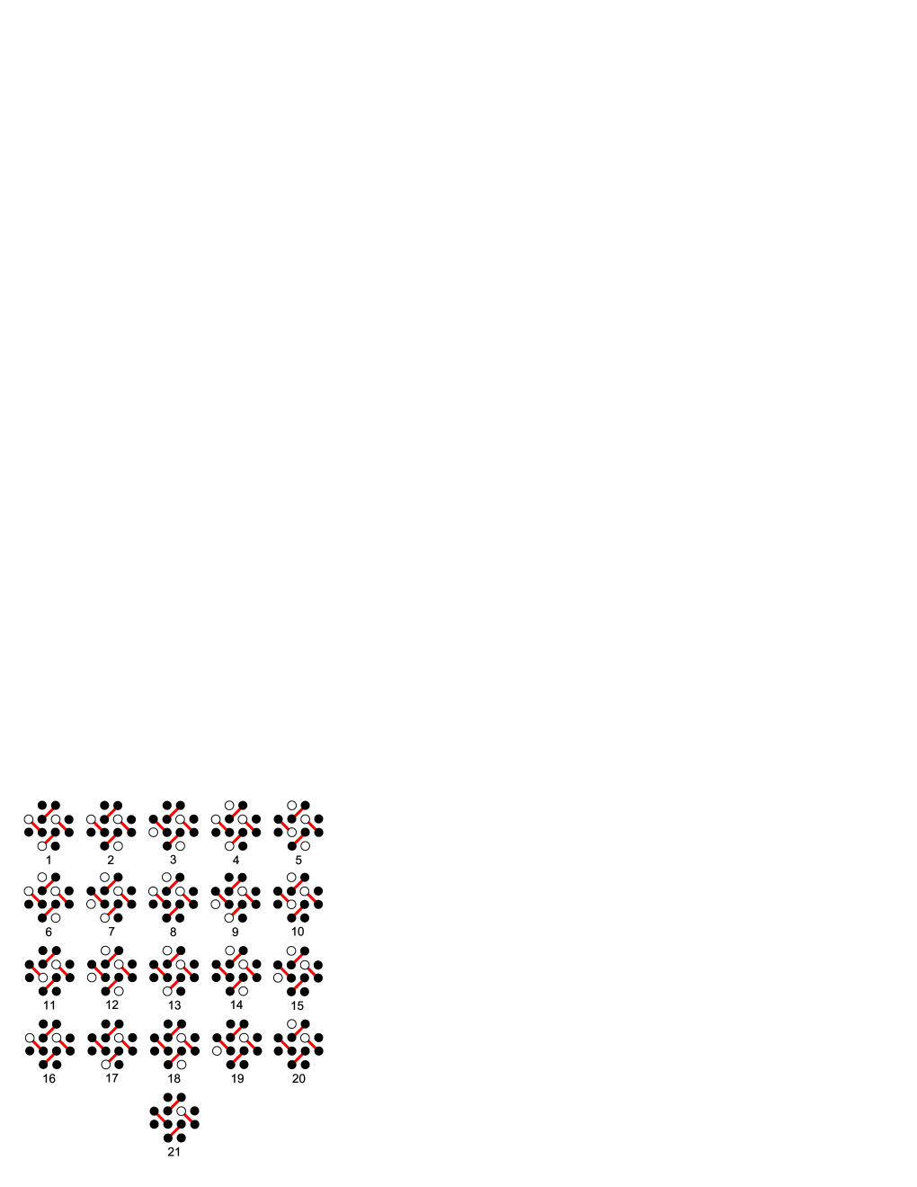
Figure 17: Configurations of the “windmill” cluster for the structures at the boundary between phases 4 and 6.

Figure 18: “Seahorse” (in red) is the maximum subcluster that can occupy two nonequivalent positions in the “windmill” cluster.

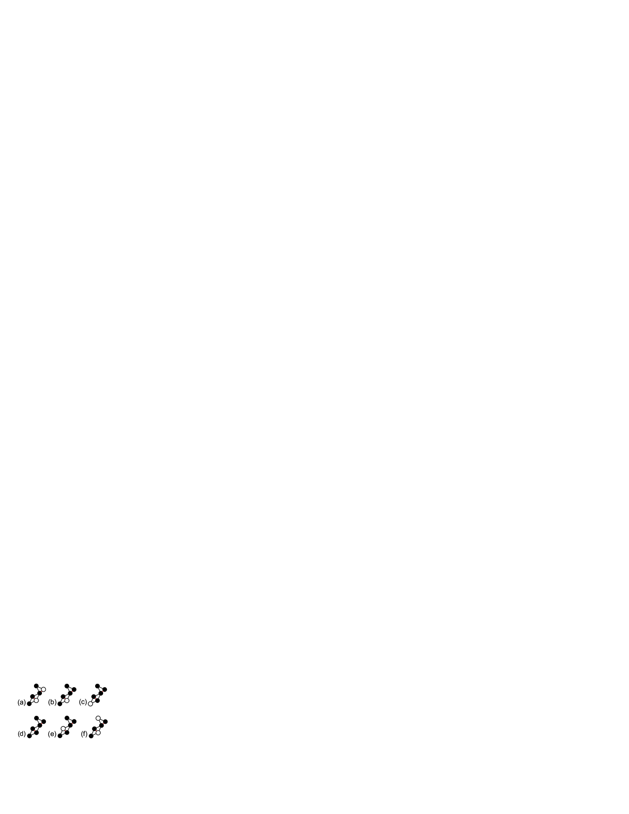
Figure 19: Some configurations of the “seahorse” subcluster.

It should be noted that in this section we use the same notations as in the previous one but here they denote other quantities. The enumeration of the cluster configurations is also different.

Consider some configurations of the maximum subcluster which can occupy two nonequivalent positions in the “windmill” cluster (Fig. 18). These configurations are shown in Fig. 19. We put the number of configurations (a) and (b) of the subcluster in different positions equal and thus obtain the relations between the fractional contents $k_{i}$ of the corresponding configurations in the structures, i.e.,

$$k_{7}+k_{9}+k_{13}+k_{17}=0,$$

$$k_{7}-k_{8}+k_{9}-k_{10}-2k_{11}+k_{13}-k_{15}$$

$$-k_{16}+k_{17}-k_{19}-k_{20}-k_{21}=0.$$ (20)

All the values of $k_{i}$ in these relations are equal to zero (since $k_{i}$ should be nonnegative). Configurations (c) and (d) lead to the relations that yield $k_{12}=0$ and $k_{18}=0$. Configurations (e) and (f) lead to the relations

$$k_{1}-k_{3}-k_{6}-k_{14}=0,$$

$$k_{1}-k_{3}+k_{4}-2k_{5}-k_{14}=0.$$ (21)

The fact that $k_{i}=0$ does not mean that the $i$th configuration cannot enter the structures (all the configurations shown in Fig. 17 can enter the structures at the boundary between phases 4 and 6). This only means that the number of such configurations is infinitesimal as compared to the number of other configurations.

The fact that the major portion of the values of $k_{i}$ are equal to zero can be proved by geometrical arguments. The fragment shown in blue in Fig. 20 generates an infinite half-stripe composed with configurations 1 and/or 4. If a configuration has two or three such fragments, then these generate the relevant number of half-stripes. For instance, configuration 15 gives rise to one half-stripe, configuration 16 generates two perpendicular half-stripes, configuration 17 also generates two half-stripes but in opposite directions, and configuration 21 even gives rise to three half-stripes (Fig. 21). Furthermore, and this is very important, different copies of these configurations on the lattice generate different copies of half-stripes. Just for this reason the number of such configurations is infinitesimal compared to the number of the rest of configurations. Similar geometrical reasoning leads to the conclusion that $k_{14}=0$, though the latter does not follow from the relations between $k_{i}$.

Figure 20: A fragment (shown in blue) which generates a half-stripe of configurations 1 and/or 4.

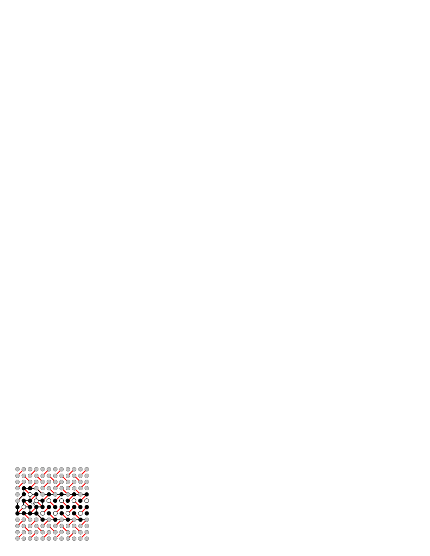
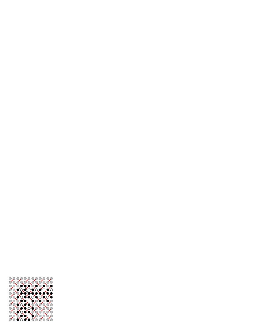
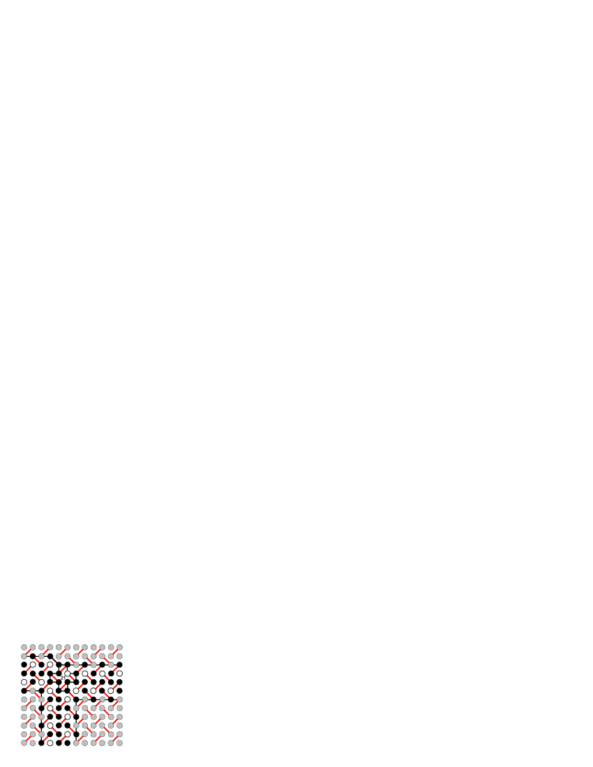
Figure 21: Half-stripes generated by configurations 15, 16, 17, and 21.

Thus, only six initial configurations have nonzero fractional contents in the ground-state structures on the boundary between phases 4 and 6. These contents satisfy the relations given by

$$k_{1}=k_{3}+k_{6},$$

$$k_{2}=-2k_{3}-3k_{5}-k_{6}+1,$$

$$k_{4}=2k_{5}-k_{6}.$$ (22)

We can exclude the configurations with $k_{i}=0$ since their number is infinitesimal. The remaining configurations generate structures of the type shown in Fig. 22. These structures represent a mixture of two kinds of stripes: one or two antiferromagnetic chains bordered by ferromagnetic ones.

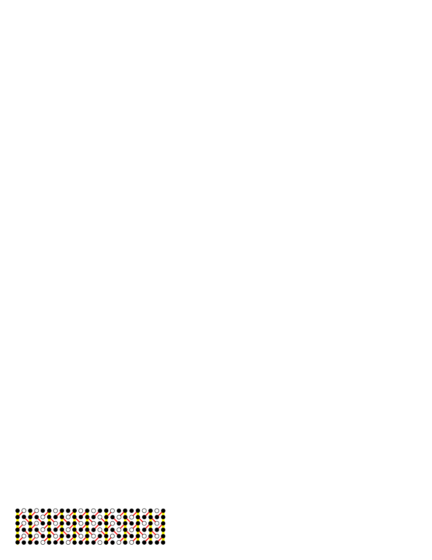
Figure 22: An example of a structure at the boundary between phases 4 and 6.

The region $ABCD$ of variation for the quantities $k_{3}$, $k_{5}$, and $k_{6}$ is shown in Fig. 23. The points $A$, $B$, and $C$ correspond to the structures $6a$, $6b$ (Fig. 24), and 4 [Fig. 4(b)], respectively. Structure $6a$ does not contain configurations 3, 5, and 6; it is generated by configuration 2. Structures $6b$ and 4 contain maximum possible numbers of configurations 3 and 5, respectively. The structure with the maximum possible number of configurations 6 corresponds to point $D$. It is shown in Fig. 25. For $0<k_{5}<\frac{1}{7}$ the maximum of $k_{6}$ at $k_{3}=0$ is determined by the number of wide stripes (as in structure 4), and for $\frac{1}{7}<k_{5}<\frac{1}{3}$ it is determined by the number of narrow stripes (as in structures $6a$ and $6b$). Similarly, for nonzero $k_{3}$: the face $ABD$ ($k_{6}=2k_{5}$, $k_{3max}=\frac{1}{2}-\frac{7}{2}k_{5}$) corresponds to the structures where each wide stripe contains configurations 6 on both sides.

The fact that the region of variation for the quantities $k_{3}$, $k_{5}$, and $k_{6}$ is the tetrahedron $ABCD$ shown in Fig. 23 can be easily proved within the context of relations (19). Thus, the last of these yields the inequality

$$k_{6}=2k_{5}-k_{4}\leqslant 2k_{5},$$ (23)

which, being taken for an equation, represents the equation of the face $ABD$ (then $k_{4}=0$). The second of relations (19) and the inequality $k_{6}-k_{2}\leqslant 0$ yield the inequality

$$2k_{3}+3k_{5}+2k_{6}-1=k_{6}-k_{2}\leqslant 0,$$ (24)

which, being taken for an equation, represents the equation of the face $BCD$ (then $k_{2}=k_{6}$). To complete the proof one should show that some structures correspond to the points $A$, $B$, $C$, and $D$. This was done before.

Figure 23: Tetrahedron of variation for the quantities $k_{3}$, $k_{5}$, and $k_{6}$.

Let us find the magnetization and the contributions to the energy density for the structures consisting of the configurations considered. The magnetization per site reads

$$m=\frac{1}{12}(6k_{1}+6k_{2}+6k_{3}+4k_{4}+4k_{5}+4k_{6})$$

$$~{}~{}~{}~{}=-\frac{1}{2}k_{5}+\frac{1}{2},$$ (25)

and the contributions of pairwise interactions to the energy density

$$e_{1}=\frac{1}{4}(-k_{1}+k_{3}-k_{4})\tilde{J}_{1}=-\frac{1}{2}k_{5}\tilde{J}_{1},$$

$$e_{2}=-2k_{5}\tilde{J}_{2},$$

$$e_{3}=k_{5}J_{3},$$

$$e_{4}=(2k_{3}+2k_{5})J_{4},$$

$$e_{5}=(k_{1}+2k_{2}+k_{3}+k_{4}+2k_{6})J_{5}$$

$$~{}~{}~{}~{}=(-2k_{3}-4k_{5}+2)J_{5},$$

$$e_{6}=\frac{1}{4}(k_{1}-k_{3}+2k_{4}+2k_{5}+k_{6})J_{6}=\frac{3}{2}k_{5}J_{6},$$

$$e_{7}=(-k_{1}+k_{3}-k_{4}+k_{5})J_{7}=-k_{5}J_{7},$$

$$e_{8}=(2k_{1}-2k_{5}-2k_{6})J_{8}=(2k_{3}-2k_{5})J_{8},$$

$$e_{9a}=\frac{1}{2}(2k_{2}-k_{4}+k_{6})J_{9}=\frac{1}{2}(-4k_{3}-8k_{5}+2)J_{9},$$

$$e_{11}=(k_{4}-k_{6})J_{11}=(2k_{5}-2k_{6})J_{11},$$

$$e_{16}=(k_{1}-k_{3}+k_{5}+k_{6})J_{16}=(k_{5}+2k_{6})J_{16}.$$ (26)

Figure 24: Structures $6a$ and $6b$. They are stabilized by ferro- and antiferromagnetic interactions of the fourth neighbors (antiferro- and ferromagnetic interactions of the fifth neighbors), respectively.

As we can follows from the above relations, the quantities $e_{1}$, $e_{2}$, and $e_{3}$ depend on $k_{5}$ only (i.e., on the magnetization $m$). Therefore, if there are no interactions other than $\tilde{J}_{1}$, $\tilde{J}_{2}$, and $J_{3}$, then the set of configurations of the “windmill” cluster (Fig. 17) generates only two full-dimensional phases: phase 4 with the maximum number of configurations 5, and phase 6 without configurations 5. The quantities $e_{6}$ and $e_{7}$ also depend on $k_{5}$ only, therefore the corresponding interactions do not lift the degeneracy at the boundary between phases 4 and 6, nor in the phase 6 itself. The quantities $e_{4}$, $e_{5}$, and $e_{8}$ depend not only on $k_{5}$ but also on $k_{3}$. Each of the corresponding interactions lifts the degeneracy of phase 6, giving rise to two new full-dimensional phases: phase $6a$ and phase $6b$ (Fig. 24). The quantities $e_{11}$ and $e_{16}$ depend on $k_{1}$ and $k_{6}$, hence the phase shown in Fig. 25 is given rise by the interactions $J_{11}$ and $J_{16}$.

The term with $k_{3}$ enters the expressions for $e_{4}$ and $e_{8}$ with the “plus” sign and the ones for $e_{5}$ — with the “minus” sign. Thus, the phase $6a$ is stabilized by the ferromagnetic interactions $J_{4}$ and $J_{8}$ as well as by the antiferromagnetic interaction $J_{5}$ (and vice versa for the phase $6b$). The term with $k_{6}$ enters the expressions for $e_{11}$ with the “minus” sign and in the expression for $e_{16}$ with the “plus” sign; therefore, the phase shown in Fig. 25 is stabilized by the antiferromagnetic interaction $J_{11}$ and by the ferromagnetic interaction $J_{16}$.

Figure 25: Structure with the maximum value of $k_{6}=\frac{2}{7}$ (the magnetization $m=\frac{3}{7}$). It emerges from the boundary between phases 4 and 6 when the interaction range reaches the 11th neighbors (three square lattice constants).

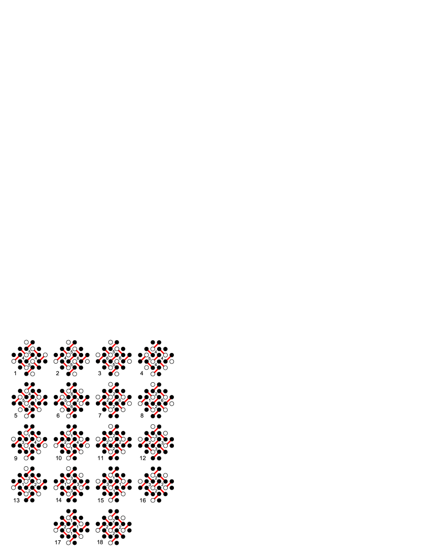
Figure 26: Configurations of the “turtle” cluster generating all the structures at the boundary between phases 4 and 6. In each “empty” square, a number of the “windmill” configuration with the center in this square is indicated.

To investigate the effect of longer-range interactions, we consider the configurations of the “turtle” cluster which generate all the structures at the boundary of phases 4 and 6. These configurations are depicted in Fig. 26. The maximum subcluster which can occupy two nonequivalent positions in the “turtle” cluster (Fig. 11) generates a set of relations for the corresponding fractional contents $l_{i}$ that is given by

$$2l_{1}+l_{2}-l_{4}-l_{5}=0,$$

$$l_{2}+2l_{3}-l_{6}=0,$$

$$l_{5}-l_{9}-l_{10}=0,$$

$$l_{6}-l_{7}-l_{8}=0,$$

$$l_{7}+l_{11}-l_{18}=0,$$

$$l_{11}+l_{13}-l_{16}-l_{18}=0,$$

$$l_{8}-l_{10}+l_{13}-l_{17}=0,$$

$$l_{9}-l_{14}+l_{15}=0,$$

$$l_{12}-l_{16}=0,$$

$$\sum\limits_{i=1}^{18}l_{i}=1.$$ (27)

The last relation is the normalization condition.

This set of equations yields

$$l_{2}=-3l_{1}+l_{3}-4l_{10}-2l_{14}-4l_{17}-2l_{18}+1,$$

$$l_{4}=-l_{1}+l_{3}-5l_{10}-3l_{14}+l_{15}-4l_{17}-2l_{18}+1,$$

$$l_{5}=l_{10}+l_{14}-l_{15},$$

$$l_{6}=-3l_{1}+3l_{3}-4l_{10}-2l_{14}-4l_{17}-2l_{18}+1,$$

$$l_{7}=-3l_{1}+3l_{3}-5l_{10}+l_{13}-2l_{14}-5l_{17}-2l_{18}+1,$$

$$l_{8}=l_{10}-l_{13}+l_{17},$$

$$l_{9}=l_{14}-l_{15},$$

$$l_{11}=3l_{1}-3l_{3}+5l_{10}-l_{13}+2l_{14}+5l_{17}+3l_{18}-1,$$

$$l_{12}=3l_{1}-3l_{3}+5l_{10}+2l_{14}+5l_{17}+2l_{18}-1,$$

$$l_{16}=3l_{1}-3l_{3}+5l_{10}+2l_{14}+5l_{17}+2l_{18}-1.$$ (28)

Hence, only eight of 18 quantities $l_{i}$ are independent.

It is easy to find the relations between the quantities $k_{i}$ ($i=1-6$) and $l_{i}$ ($i=1-18$). We just have to calculate the numbers of configurations of the “windmill” subcluster in configurations of the “turtle” cluster. Thus we have

$$4k_{1}=l_{5}+l_{8}+2l_{9}+2l_{10}+l_{13}+l_{14}+3l_{15}+3l_{17},$$

$$~{}~{}~{}~{}~{}=4(l_{10}+l_{14}+l_{17}),$$

$$4k_{2}=l_{6}+3l_{7}+2l_{8}+l_{10}+4l_{11}+l_{12}+3l_{13}$$

$$~{}~{}~{}+3l_{16}+l_{17}+4l_{18},$$

$$4k_{3}=l_{9}+3l_{12}+3l_{14}+l_{15}+l_{16}$$

$$~{}~{}~{}~{}=4(3m-1)-4(l_{10}+l_{17}+l_{18}),$$

$$4k_{4}=2l_{1}+l_{2}+3l_{4}+2l_{5}+l_{9}+l_{10},$$

$$4k_{5}=2l_{1}+2l_{2}+2l_{3}+l_{4}+l_{5}+l_{6},$$

$$4k_{6}=l_{2}+2l_{3}+2l_{6}+l_{7}+l_{8}.$$ (29)

Within the context of these and previous relations, we can write the contributions into the energy density for the pairwise interactions which (except for $J_{11}$ and $J_{16}$) are not contained in the “windmill” cluster, i.e.,

$$e_{9}=(-4k_{3}-8k_{5}+2)J_{9},$$

$$e_{10}=k_{5}J_{10},$$

$$e_{11}=(2k_{5}-2k_{6})J_{11},$$

$$e_{12}=(2k_{3}+6k_{5}-2k_{6})J_{12},$$

$$e_{13}=(-k_{5}+2k_{6})J_{13},$$

$$e_{14}=-\frac{1}{2}k_{5}J_{14},$$

$$e_{15}=(4k_{3}-2k_{5}+4k_{6}-4l_{14})J_{15},$$

$$e_{16}=(k_{5}+2k_{6})J_{16},$$

$$e_{17}=(2k_{3}+2k_{5}-2k_{6})J_{17},$$

$$e_{18}=(-4k_{3}-4k_{5}-2k_{6}+4l_{14}+2)J_{18},$$

$$e_{21}=(k_{5}-k_{6}+l_{3})J_{21},$$

$$e_{25}=(-\frac{1}{2}k_{5}+2k_{6})J_{25}.$$ (30)

Pairwise interactions up to the 14th neighbors as well as many-spin interactions which correspond to the clusters that include only neighbors up to 14th range cannot give rise to any full-dimensional structure from the boundary between phases 4 and 6 except for the four structures mentioned above. The reason is that the contributions to the energy density $e_{i}$ ($i=1-14$) depend on $k_{3}$, $k_{5}$, and $k_{6}$ only. On the contrary, the contributions $e_{15}$ and $e_{18}$ depend also on $l_{14}$; therefore, the corresponding interactions can give rise to new full-dimensional structures. It should be noted that the 15th-neighbor interaction is an interaction of chains at the distance of four square lattice constants.

Since the structures at the boundary between phases 4 and 6 are striped, the identical configurations are organized in stripes. Therefore, a structure can be described by a sequence of “windmill” configurations.

Let us find new full-dimensional structures that can be given rise by the 15th-neighbor interaction. The expression for $e_{15}$ can be rewritten in terms of $k_{1}$, $k_{5}$, and $l_{14}$. The polyhedron of variation for these quantities is shown in Fig. 27. Vertices $A$, $B$, $C$, and $D$ correspond to the structures similar to those in Fig. 23; vertex $E$ corresponds to the structure shown in Fig. 28. Let us prove that the pyramid $ABCDE$ is indeed the region of variation for the quantities $k_{1}$, $k_{5}$, and $l_{14}$ in the relevant space.

It is easy to show that $k_{1}$ and $k_{5}$ vary within the triangle $ACM$. With this observation in view, we just have to prove that the points with maximum (minimum) values of $l_{14}$, for fixed $k_{1}$ and $k_{5}$, are the points of the triangle $ABC$ [of the quadrangle $ACDE$ ($l_{14}=0$) and triangle $BDE$].

For fixed values of $k_{1}$ and $k_{5}$, the value of $l_{14}$ reaches the maximum in the structures where each column of the “windmill” configurations 1 has two neighbor columns of configurations 3 (if the number of configurations 5 makes it possible); then $l_{14}=k_{1}$ (the face $ABC$ in Fig. 27).

Let the number of “windmill” configurations 1 and 5 be equal to $N_{1}$ and $N_{5}$, respectively. Then the number of configurations 1 can exceed the number of configurations 3 by $2N_{5}$ at the most. (If there are no configurations 5, then the number of configurations 3 is equal to the number of configurations 1.) The number of the rest $N_{1}-2N_{5}$ configurations 1 together with similar number of configurations 3 and similar number of configurations 2 is equal to $N-7N_{5}$, where $N$ is the total number of “windmill” configurations in the structure. If the number of configurations 2 is at least twice greater than the number of configurations 3, then configurations 1 and 3 can be separated by configurations 2 so that no combinations 133 appear (then $l_{14}=0$). Then the number of configurations 1 cannot exceed $2N_{5}+\frac{1}{4}(N-7N_{5})$. Each excessive configuration 1 inevitably leads to the appearance of two “turtle” configurations 14. Hence, the minimum number of configurations 14 is given by

$$l_{14}=2\left[k_{1}-\left(2k_{5}+\frac{1}{4}(1-7k_{5})\right)\right]$$

$$~{}~{}~{}=2k_{1}-\frac{k_{5}+1}{2}.$$ (31)

This is just the equation of the face $BDE$.

The equation of the face $ABC$ can be obtained in a similar manner. The first of Eqs. (20) can be rewritten in the form

$$l_{14}=k_{1}-l_{10}-l_{17},$$ (32)

whence it follows that

$$l_{14}\leqslant k_{1}.$$ (33)

The relation that yields the equation of the face $ABC$ is obtained under the condition $l_{10}=l_{17}=0$.

The face $BDE$ gives the inequality

$$4k_{1}-k_{5}-2l_{14}-1\leqslant 0.$$ (34)

Using the relations for $l_{i}$ and $k_{i}$, this inequality can be reduced to

$$2l_{1}+l_{2}+l_{18}\geqslant 0.$$ (35)

This proves that the face $BDE$ was obtained correctly and in this face $l_{1}=l_{2}=l_{18}=0$. The relations for $l_{i}$ yield also $l_{4}=l_{5}=l_{7}=l_{9}=l_{10}=l_{11}=0$.

Hence, the 15th-neighbor anfiferromagnetic interaction gives rise to the structure shown in Fig. 28. This structure has the number of ferro- and antiferromagnetic SS dimers similar to the 1/2-plateau structure proposed in Ref. bib14, . However, the dimensions of their unit cells are different: 8 and 16 square lattice constants, respectively; ferro- and antiferromagnetic chains are also distributed differently.

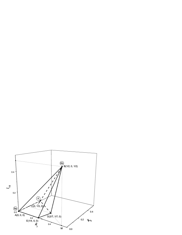
Figure 27: Polyhedron of variation for the quantities $k_{1}$, $k_{5}$, and $l_{14}$. Each vertex corresponds to a full-dimensional structure.

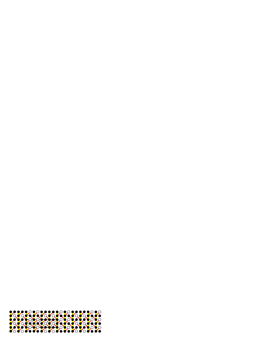
Figure 28: The structure given rise by the antiferromagnetic 15th-neighbor interaction from the boundary between phases 4 and 6. This structure possesses maximum number of “windmill” configurations 1 (or 3) with no “windmill” configurations 5 and “turtle” configurations 14.

IV Full-dimensional ground-state structure emerging from the boundary between phases 1 and 6

All the structures at the boundary between phases 1 and 6 consist of the configurations of squares , , , ; , and , or with the set of configurations of the “screw” cluster shown in Fig. 29. In addition to the normalization condition, there are three relations for the fractional contents $p_{i}$ ($i=$1-10) of these configurations. It is easy to derive them, by considering the configurations of the maximum subcluster which can occupy two nonequivalent positions in the “screw” cluster (Fig. 30).

$$p_{4}-p_{7}+2p_{8}+4p_{10}=0,$$

$$p_{2}-p_{3}+p_{4}+2p_{5}+p_{7}+p_{8}+p_{9}=0,$$

$$\sum\limits_{i=1}^{10}p_{i}=1.$$ (36)

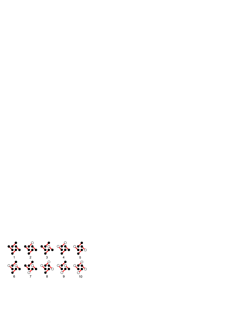
Figure 29: Configurations of the “screw” cluster for the boundary between phases 1 and 6.

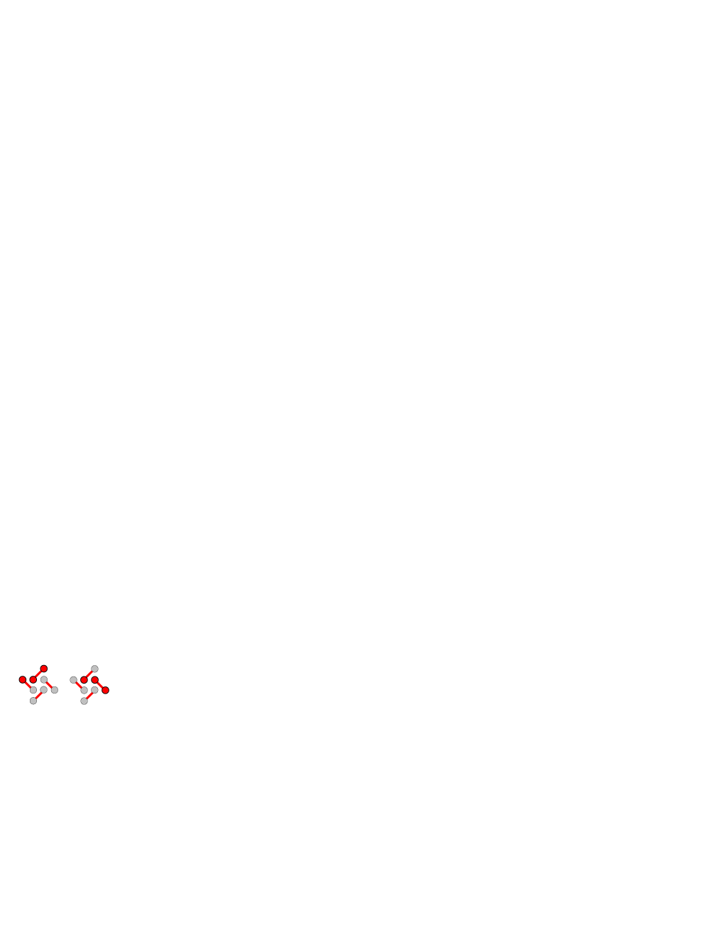
Figure 30: The maximum subcluster that can occupy two nonequivalent positions in the “screw” cluster.

Let us find the magnetization per site, taking into account that two sites are the share of each of the “screw” clusters on the lattice

$$m=\frac{1}{2}(2p_{1}+2p_{2}+p_{3}+2p_{4}+2p_{5}+p_{6}+p_{7}+2p_{8}$$

$$~{}~{}~{}~{}~{}+p_{9}+2p_{10})=\frac{1}{2}(2-p_{3}-p_{6}-p_{7}-p_{9}).$$ (37)

The contributions into the energy density of pairwise interactions within the “screw” cluster are given by

$$e_{1}=\frac{1}{8}(4p_{1}+2p_{2}+2p_{3}-2p_{8}-2p_{9}-4p_{10})\tilde{J}_{1}$$

$$~{}~{}~{}~{}=(m-\frac{1}{2})\tilde{J}_{1},$$

$$e_{2}=\frac{1}{2}(4p_{1}+4p_{2}+4p_{4}+4p_{5}+4p_{8}+4p_{10})\tilde{J}_{2}$$

$$~{}~{}~{}~{}=2(2m-1)\tilde{J}_{2},$$

$$e_{3}=\frac{1}{2}(2p_{1}+2p_{2}+2p_{4}+2p_{5}+2p_{8}+2p_{10})J_{3}$$

$$~{}~{}~{}~{}=(2m-1)J_{3},$$

$$e_{4}=\frac{1}{2}(4p_{1}+2p_{2}+2p_{3}+4p_{7}-2p_{8}+2p_{9}-4p_{10})J_{4}$$

$$~{}~{}~{}~{}=2(1-p_{3}-p_{6})J_{4},$$

$$e_{5}=\frac{1}{2}(4p_{1}+2p_{2}+2p_{3}+4p_{6}-2p_{8}+2p_{9}-4p_{10})J_{5}$$

$$~{}~{}~{}~{}=2(1-p_{3}-p_{7})J_{5},$$

$$e_{7}=(p_{1}+p_{3}-p_{4}+p_{5}-p_{9}+p_{10})J_{7}$$

$$~{}~{}~{}~{}=[4m-3+(p_{3}+p_{6})+(p_{3}+p_{7})$$

$$~{}~{}~{}~{}-(p_{2}+2p_{4}+p_{8})]J_{7}.$$ (38)

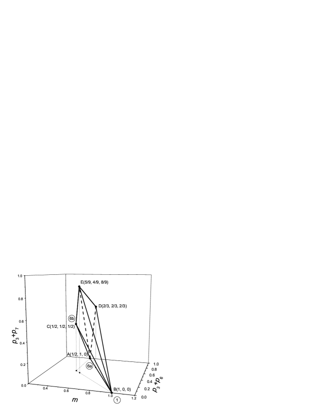
Figure 31: Polyhedron of variation for the quantities $m$, $p_{3}+p_{6}$, and $p_{3}+p_{7}$.

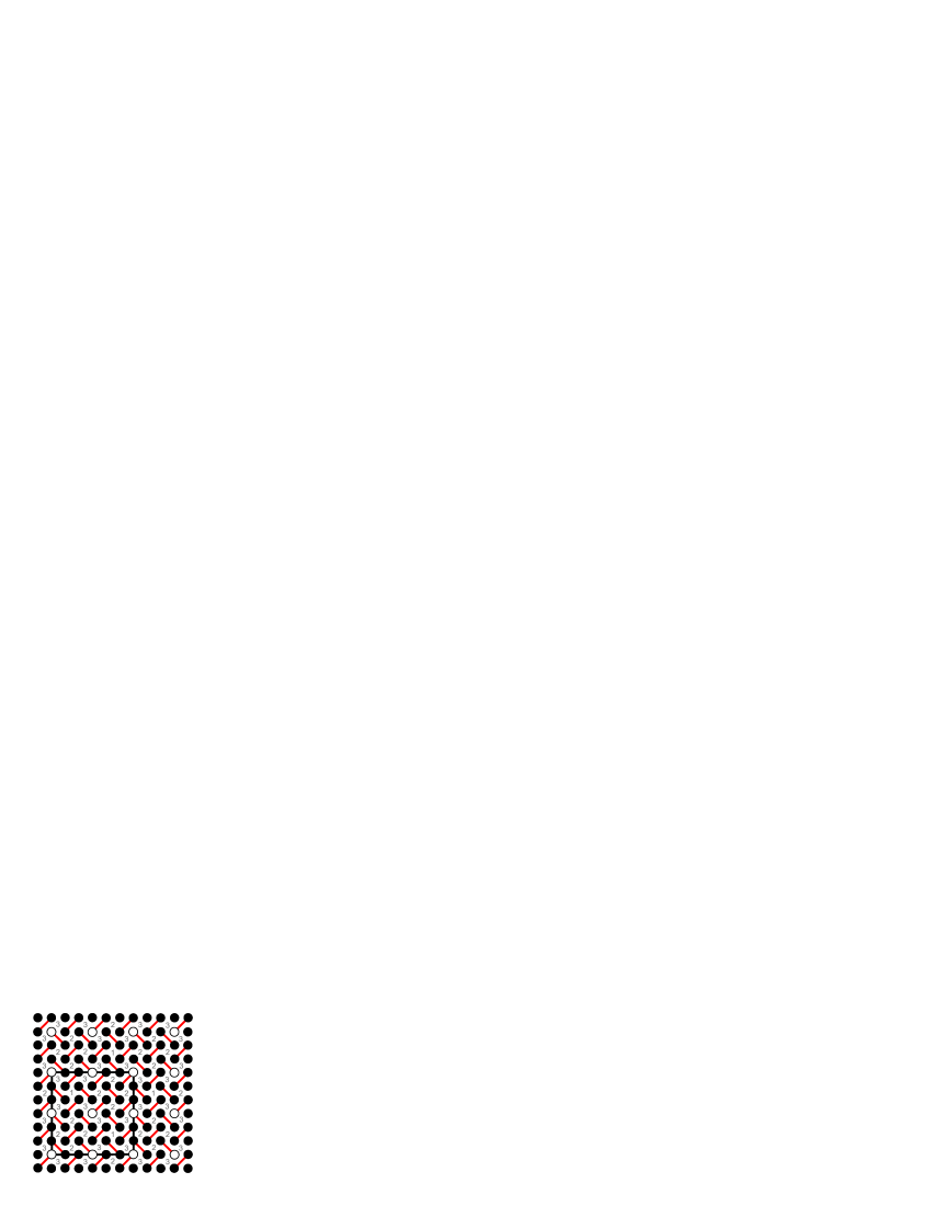
Figure 32: A structure emerging from the boundary between phases 1 and 6. It corresponds to the vertex $D$ for which $p_{3}=\frac{1}{2}$, $p_{7}=\frac{1}{3}$, $p_{8}=\frac{1}{6}$; and $m=\frac{2}{3}$.

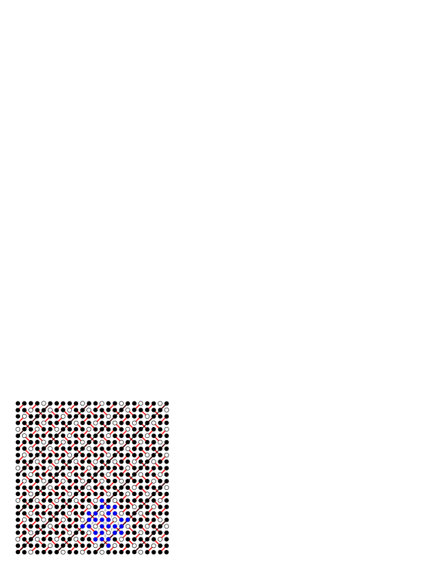
Figure 33: Partially disordered structure emerging from the boundary between phases 1 and 6. It corresponds to the vertex $E$ for which $p_{3}=p_{7}=\frac{4}{9}$, $p_{10}=\frac{1}{9}$; and $m=\frac{5}{9}$.

The region of variation for the quantities $m$, $p_{3}+p_{6}$, and $p_{3}+p_{7}$ is the polyhedron $ABCDE$ shown in Fig. 31. It is described by the set of inequalities

$$ABC:2m+(p_{3}+p_{6})+(p_{3}+p_{7})-2\geqslant 0,$$

$$ABD:2m+(p_{3}+p_{6})-2\leqslant 0,$$

$$BCE:m+(p_{3}+p_{6})-1\geqslant 0,$$

$$BDE:2m+(p_{3}+p_{7})-2\leqslant 0,$$

$$ACE:6m-(p_{3}+p_{6})-(p_{3}+p_{7})-2\geqslant 0,$$

$$ADE:2m-3(p_{3}+p_{6})-2(p_{3}+p_{7})+2\geqslant 0.$$ (39)

These inequalities are rather difficult to find but easy to prove using the expression for $m$ and the relations for $p_{i}$. For instance, the inequality

$$2m+p_{3}+p_{6}-2\leqslant 0$$ (40)

immediately follows from the expression (37) for $m$. It becomes an equation if $p_{7}=p_{9}=0$.

When proving the inequalities, we find that at faces some of quantities $p_{i}$ are equal to zero. We have

$$ABC:p_{2}=p_{4}=p_{5}=p_{7}=p_{8}=0,~{}~{}p_{10}=0;$$

$$ABD:p_{7}=p_{9}=0;$$

$$BCE:p_{2}=p_{4}=p_{5}=p_{6}=p_{8}=0;$$

$$BDE:p_{6}=p_{9}=0;$$

$$ACE:p_{1}=p_{2}=p_{4}=p_{5}=p_{8}=0;$$

$$ADE:p_{1}=p_{2}=p_{4}=p_{9}=0.$$ (41)

The ground-state structures for the edges of the polyhedron $ABCDE$ are constructed with the following configurations of the “screw” cluster:

$$AB:1,3,6;~{}AC:3,6,9;~{}AD:3,5,6;$$

$$AE:3,6,7,10;~{}BC:1,3,9;$$

$$BD:1,2,3,4,5,8,10;~{}BE:1,3,7,10;$$

$$CE:3,7,9,10;~{}DE:3,5,7,8,10.$$ (42)

At the vertex $E$, four faces converge: $BCE$, $BDE$, $ACE$, and $ADE$, or edges $AE$, $BE$ , $CE$, and $DE$. Thus, the ground-state structures in this vertex consist of configurations 3, 7, and 10 of the “screw” cluster. For this vertex, Eqs. (33) reduce to the set

$$p_{7}-4p_{10}=0,$$

$$-p_{3}+p_{7}=0,$$

$$p_{3}+p_{7}+p_{10}=1.$$ (43)

The solution of this set of equations is $p_{3}=\frac{4}{9}$, $p_{7}=\frac{4}{9}$, $p_{10}=\frac{1}{9}$. The structure which corresponds to the vertex $E$ is shown in Fig. 32.

At the vortex $D$ three faces converge: $ABD$, $BDE$, and $ADE$, or edges $AD$, $BD$, and $ED$. Thus, the ground-state structures in this vertex consist of configurations 3 and 5 of the “screw” cluster. For this vertex, Eqs. (33) reduce to the set

$$-p_{3}+2p_{5}=0,$$

$$~{}~{}~{}p_{3}+p_{5}=1.$$ (44)

The solution of this set of equations is $p_{3}=\frac{2}{3}$, $p_{5}=\frac{1}{3}$. The structure which corresponds to the vertex $D$ is shown in Fig. 33.

For $6a$ $p_{6}=1$, and for $6b$ $p_{3}=p_{9}=\frac{1}{2}$. In the face $ABC$ $p_{3}=p_{9}$, $p_{2}=p_{4}=p_{5}=p_{8}=p_{10}=0$.

$$k_{2}-k_{4}+2k_{5}+k_{7}+k_{8}+k_{9}+k_{12}-k_{13}-k_{15}$$

$$+k_{16}+k_{18}+k_{19}+k_{20}=0,$$

$$k_{8}-k_{12}+2k_{16}+k_{18}+4k_{26}+k_{28}=0,$$

$$k_{3}-k_{4}+2k_{6}+k_{7}+k_{9}+k_{10}-k_{11}-k_{12}-k_{14}$$

$$+k_{15}+k_{17}+k_{18}+k_{19}-k_{20}+k_{22}=0,$$

$$k_{10}-k_{15}+2k_{17}+k_{19}-k_{22}+4k_{27}=0,$$

$$k_{13}-k_{14}+k_{21}+k_{23}-k_{25}+k_{28}=0.$$ (45)

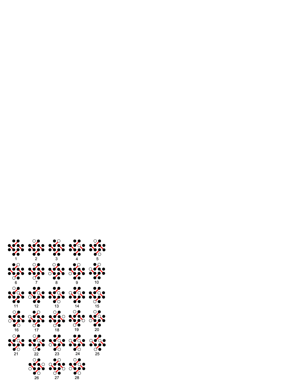
Figure 34: Configurations of the “windmill” cluster for the boundary between phases 1 and 6.

V Full-dimensional ground-state structures emerging from the boundary between phases 3 and 7

The 1/9-plateau structure and other structures of this type that have been observed experimentally in Ref. bib14 are the ground-state structures at the boundary between phases 3 and 7. Hence, it is interesting to investigate which full-dimensional structures from this boundary are produced by the extended-range interactions. All the structures at this boundary consist of two configurations of the “screw” cluster (see Fig. 35) or with the square configurations , , , ; , and . Only one relation between fractional contents $p_{1}$ and $p_{2}$ of “screw” configurations in structures (the normalization condition) holds, i.e.,

$$p_{1}+p_{2}=1.$$ (46)

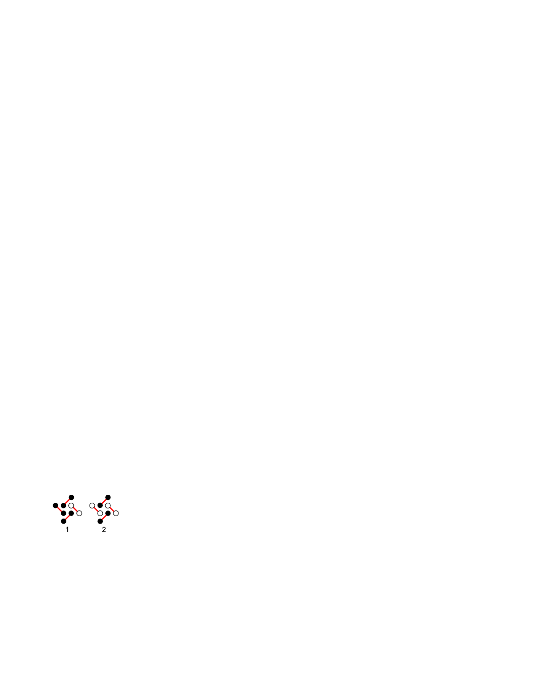
Figure 35: Configurations of the “screw” cluster at the boundary between phases 3 and 7.

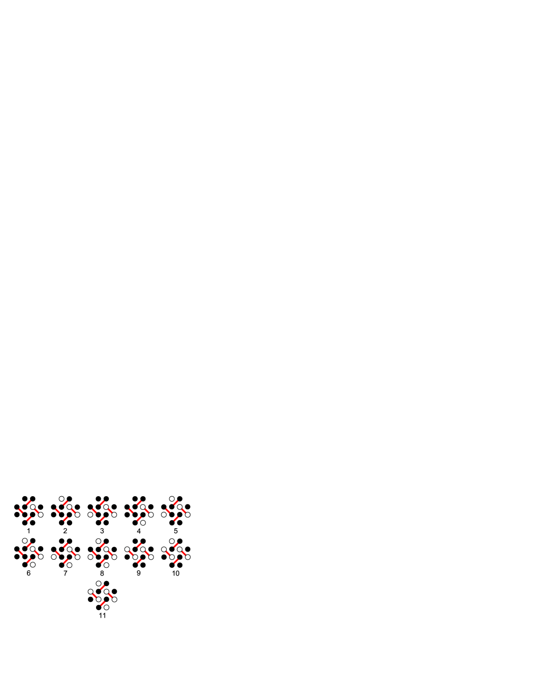
Figure 36: Configurations of the “windmill” cluster for the boundary between phases 3 and 7.

Now, let us consider a bigger cluster, the “windmill” cluster, and its configurations generating all the ground-state structures at the boundary between phases 3 and 7 (Fig. 36). An example of a structure at this boundary is shown in Fig. 37. The number of the “windmill” configuration with the center in an ”empty” square is indicated in each of these. Considering configurations of the “seahorse” subcluster yields the relations between the fractional contents $k_{i}$ of the “windmill” configurations in structures, i.e.,

$$k_{8}=k_{3},$$

$$k_{1}-k_{3}+k_{4}-k_{5}=0,$$

$$k_{4}+k_{6}+k_{7}+k_{8}-2k_{9}-k_{10}=0.$$ (47)

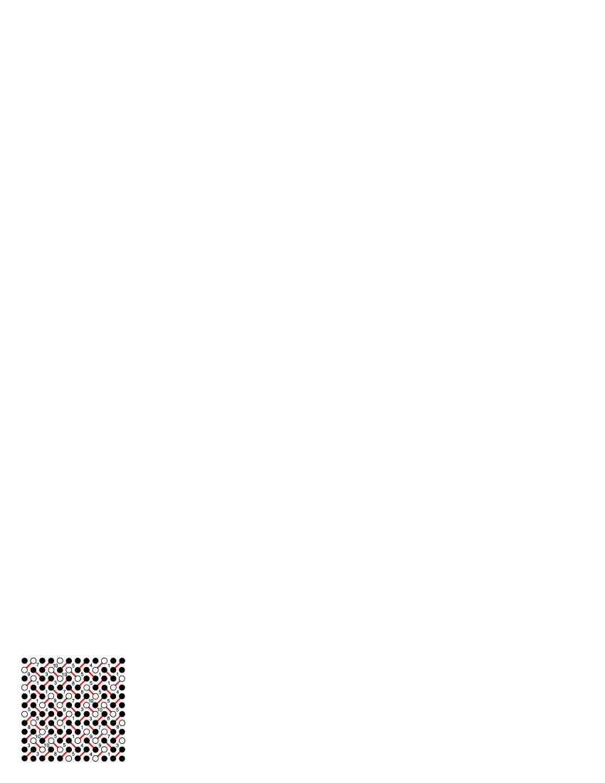
Figure 37: An example of a structure at the boundary between phases 3 and 7. The number of the “windmill” configuration in an “empty” square with the center in this square is indicated in each such square. $k_{1}=k_{5}=\frac{1}{5}$, $k_{3}=k_{4}=k_{7}=k_{8}=k_{9}=k_{10}=\frac{1}{10}$.

It is easy to find relations between the quantities $p_{1}$, $p_{2}$, and $k_{i}$. We have

$$p_{1}=k_{1}+k_{2}+k_{3}+k_{4}+k_{5}+k_{6}+k_{7}+k_{8},$$

$$p_{2}=k_{9}+k_{10}+k_{11}.$$ (48)

The magnetization and the contributions into the energy density of pairwise interactions within the “windmill” cluster are given by

$$m=\frac{p_{1}}{2},$$

$$e_{1}=\frac{\tilde{J}_{1}}{2},$$

$$e_{2}=-2p_{2}\tilde{J}_{2}=(4m-2)\tilde{J}_{2},$$

$$e_{3}=p_{2}J_{3}=(-2m+1)J_{3},$$

$$e_{4}=-2p_{2}J_{4}=(4m-2)J_{4},$$

$$e_{5}=2p_{2}J_{5}=(-4m+2)J_{5},$$

$$e_{6}=\frac{1}{4}(k_{1}+2k_{2}+k_{5}+k_{6}-k_{7}+k_{10}+2k_{11})J_{6}$$

$$~{}~{}~{}~{}=\frac{1}{2}(-k_{5}-k_{7}-2k_{8}-2k_{9}-k_{10}+1)J_{6}$$

$$~{}~{}~{}~{}=\frac{1}{2}\left[-(k_{5}+k_{7}+2k_{8})+(k_{10}+2k_{11})+4m-1\right]J_{6},$$

$$e_{7}=p_{2}J_{7}=(-2m+1)J_{7},$$

$$e_{8}=2(k_{1}+2k_{3}+k_{5}-k_{6}+k_{7}-k_{10}-2k_{11})J_{8}$$

$$~{}~{}~{}~{}=2(k_{5}+k_{7}+2k_{8}-k_{9}-k_{10}-k_{11})J_{8}$$

$$~{}~{}~{}~{}=2(k_{5}+k_{7}+2k_{8}+2m-1)J_{8},$$

$$e_{9a}=\frac{1}{2}(k_{1}+2k_{2}+k_{5}+k_{6}-k_{7}+k_{10}+2k_{11})J_{9}$$

$$~{}~{}~{}~{}=\left[-(k_{5}+k_{7}+2k_{8})+(k_{10}+2k_{11})+4m-1\right]J_{9},$$

$$e_{11}=(k_{1}+2k_{3}+k_{5}-k_{6}+k_{7}-k_{10}-2k_{11})J_{11}$$

$$~{}~{}~{}~{}~{}=(k_{5}+k_{7}+2k_{8}+2m-1)J_{11},$$

$$e_{16}=(k_{1}-k_{5}+k_{6}-k_{7}+k_{9}+k_{11})J_{16}$$

$$~{}~{}~{}~{}~{}=(-2k_{2}-4k_{5}-2k_{7}-4k_{8}$$

$$~{}~{}~{}~{}~{}~{}~{}~{}~{}-3k_{9}-3k_{10}-k_{11}+2)J_{16}.$$ (49)

Structure 3 consists of configurations 11 and structure 7 of configurations 1, 2, and 5. The 6th (and also 9ath) neighbor interaction lifts the degeneracy of phase 7, the structures $7a$ and $7b$ (Fig. 38) thus become full-dimensional for $J_{6}>0$ and $J_{6}<0$, respectively (and vice versa for the 8th neighbor interaction ). For $7a$, we have $k_{1}=k_{5}=\frac{1}{2}$. For $7b$, we have $k_{2}=1$. For $J_{6}$ the expression attains its minimum value for the structure $4a$ that consist of configurations 7 and 9 ($k_{7}=\frac{2}{3}$, $k_{9}=\frac{1}{3}$).

It follows from the inequality

$$2m=p_{1}=k_{1}+k_{2}+...+k_{8}\geqslant k_{5}+k_{7}+2k_{8}$$ (50)

that the quantity $k_{5}+k_{7}+2k_{8}$ cannot exceed $2m$. It is equal to $2m$ for the structures formed by stripes which consist of even numbers of antiferromagnetic chains between two ferromagnetic ones.

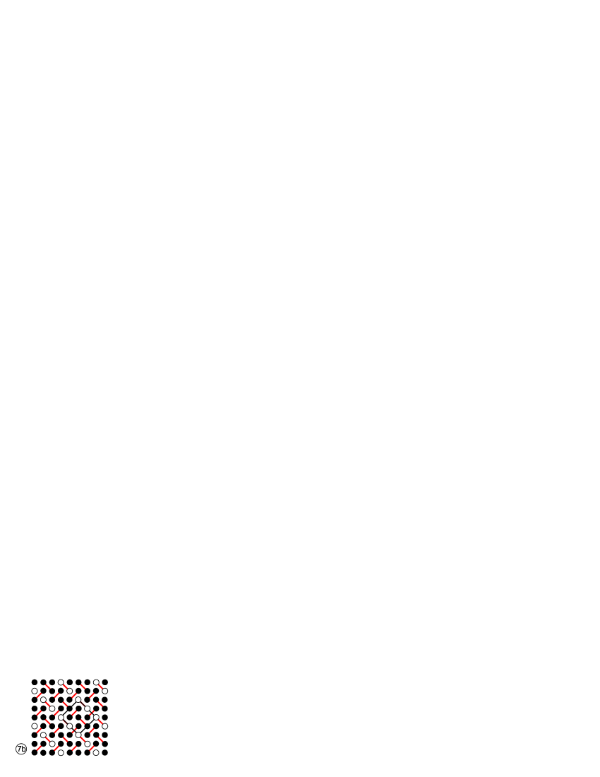
Figure 38: Structures $7a$, $7b$, and $4a$.

Figure 39: Polygon of variation for the quantities $k_{5}+k_{7}+2k_{8}$, and $m$. Its vertices correspond to the structures shown in Fig. 37 and the Néel structure 3.

Figure 40: An example of a structure at the boundary between phases 3 and 7. The structure of this kind of structures can be treated as a simple mixture of structures 3 and $4a$. The number of the “windmill” configuration with the center in an ”empty” square is indicated in each square.

For “pure” structures, where all stripes are identical, the magnetization and the values of $k_{i}$ are given by

$$m=\frac{1}{2n+3},$$

$$k_{7}=k_{10}=\frac{2}{2n+3},~{}k_{11}=\frac{2n-1}{2n+3},$$ (51)

where $2(n+1)$ $(n=1,...)$ are the numbers of antiferromagnetic chains in the stripes. The structures of this type with fractional values of magnetization $m=1/7,1/9,1/11$ and some others have been observed experimentally in TmB₄ bib14 . These structures are generated by the set of square configurations , , ; , and (without configuration ), or the equivalent set of configurations 7-11 of the “windmill” cluster.(There can be no more than two configurations 8 in a structure; such a configuration emerges when an extreme ferromagnetic chain forms a right angle.) These structures are very similar to the structures at the boundary between phases 3 and 4, however, their antiferromagnetic chains are shifted.

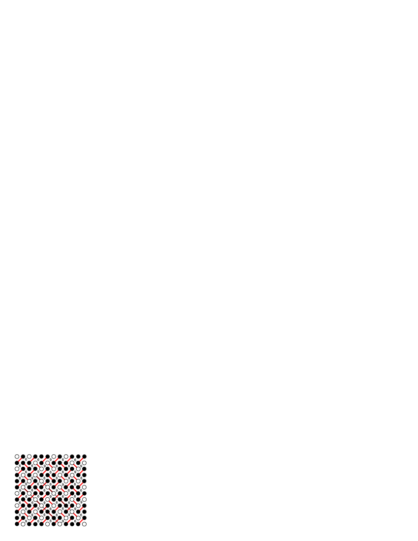
Figure 41: The structure at the boundary between phases 3 and 7 which corresponds to the vertex $E$ of the polyhedron $ABCDE$. Each “empty” square is labeled by the number of the “windmill” configuration with the center in this square. The structure is generated by the “windmill” configurations 9 and 6 ($k_{6}=\frac{2}{3}$, $k_{9}=\frac{1}{3}$).

Figure 42: Polyhedron of variation for the quantities $k_{5}+k_{7}+2k_{8}$ and $k_{10}+2k_{11}$. Its vertices correspond to the structures shown in Figs. 38 and 41 and the Néel structure 3.

The structure shown in Fig. 42 is given rise by the interactions of sixth and eighth neighbors, though each of these interactions separately cannot produce this structure. It mixes with structures 3, $7a$, and $7b$.

The expression for $m$ and the relations between $k_{i}$ yield the equation

$$k_{10}+2k_{11}=2(1-2m)-2k_{9}-k_{10}$$

$$~{}~{}~{}~{}~{}~{}~{}~{}=2(1-2m)-(k_{4}+k_{6}+k_{7}+k_{8})$$

$$~{}~{}~{}~{}~{}~{}~{}~{}=2(1-3m)+(k_{1}+k_{2}+k_{3}+k_{5}),$$ (52)

whence it follows that

$$2(1-2m)\leqslant k_{10}+2k_{11}\leqslant 2(1-3m).$$ (53)

Now we just have to prove that the following inequality holds:

$$m+(k_{5}+k_{7}+2k_{8})+\frac{1}{2}(k_{10}+2k_{11})-1\leqslant 0,$$ (54)

which, when taken for an equation is the equation of face $ACD$. Using the expression for $m$ and the relations between $k_{i}$, we can transform this inequality into

$$k_{2}+k_{4}+2k_{6}\geqslant 0,$$ (55)

The latter holds because $k_{i}\geqslant 0$. Thus, we have proved that the polyhedron $ABCDE$ (Fig. 42) is the region of variation for the quantities $m$, $k_{5}+k_{7}+2k_{8}$, and $k_{10}+2k_{11}$. In the face $ACD$, we have $k_{2}=k_{4}=k_{6}=0$.

VI Conclusions

We employ the relations for the fractional contents of the cluster configurations in the structures generated by these configurations to proposed a way to reveal the interactions which lift the degeneracy at the boundary between the full-dimensional ground-state phases and to construct the full-dimensional structures which emerge consequently. We consider several boundaries between full-dimensional ground-state phases for the system of Ising spins on the Shastry-Sutherland lattice in a magnetic field with the first-, second, and third-neighbor interactions.

The seventh-neighbor interaction (one of the interactions between chains at the distance of three square lattice constants on the SS lattice) can partially lift the degeneracy between the Néel phase and the 1/3-plateau phase giving rise to a full-dimensional structure with the magnetization 1/5. The 21th neighbor interaction (corresponding to the distance of five square lattice constants) can generate a full-dimensional structure with the magnetization 1/7. The 1/7 plateau as well as 1/9 and 1/11 plateaus were observed in TmB₄. The 1/9 and 1/11 plateaus can emerge from the boundary between the Néel phase and the 1/3-plateau phase only provided the interaction between the chains at the distances of seven and nine square lattice constants, respectively, has begun.

VII Acknowledgments

The author is grateful to I. Stasyuk and T. Verkholyak for useful discussions and suggestions and to O. Kocherga for correction of the text.

References

(1) G.H. Wannier, Phys. Rev. 79, 357 (1950).
(2) A. Danielian, Phys. Rev. Lett. 6, 670 (1961).
(3) J. Kanamori, Prog. Theor. Phys. 35, 16 (1966).
(4) T. Morita, J. Phys. A: Math., Nucl. Gen. 7, 289 (1974).
(5) U. Brandt and J. Stolze, Z. Phys. B: Condens. Matter 64, 481 (1986).
(6) T. Kennedy, Rev. Math. Phys. 6, 901 (1994).
(7) Yu.I. Dublenych, Phys. Rev. E 80, 011123 (2009).
(8) Yu.I. Dublenych, Phys. Rev. E 84, 011106 (2011).
(9) Yu.I. Dublenych, Phys. Rev. E 84, 061102 (2011).
(10) Yu.I. Dublenych, Phys. Rev. B 86, 014201 (2012).
(11) Yu.I. Dublenych, Phys. Rev. Lett. 109, 167202 (2012).
(12) Yu.I. Dublenych, Phys. Rev. E 88, 022111 (2013).
(13) Yu.I. Dublenych, Phys. Rev. E 83, 022101 (2011).
(14) K. Siemensmeyer, E. Wulf, H.-J. Mikeska, K. Flachbart, S. Gabáni,
S. Mat’aš, P. Priputen, A. Efdokimova, and N. Shitsevalova,
Phys. Rev. Lett. 101, 177201 (2008).
(15) S. Mat’aš et al., J. Phys: Conf. Ser. 200, 032041 (2010).