3D EFFECTS OF THE ENTROPIC FORCE

Abstract

This work analyzes the classical statistical mechanics associated to phase-space curves in three dimensions. Special attention is paid to the entropic force. Strange effects like confinement, hard core, and asymptotic freedom are uncovered. Negative specific heats, that were previously seen to emerge in a one-dimensional setting, disappear in 3D, and with them, gravitational effects of the entropic force.

Keywords: Phase-space curves, Entropic force, Confinement, Hard core, Asymptotic freedom.

1 Introduction

A previous one-dimensional study concerning the classical statistical mechanics of arbitrary phase-space curves $\Gamma$ [1] was shown to uncover some strange (for a classical setting), like confinement and asymptotic freedom. Of course, by confinement one alludes to the physical phenomenon that impedes isolation of color charged particles (such as quarks), that cannot be isolated singularly, while asymptotic freedom is a property of some gauge theories that originates bonds between particles to become asymptotically weaker as distance decreases.

The classical analysis of [1] provided a simple entropic mechanism for these “strange” phenomena. Remind the reader that the entropic force is a phenomenological one arising from some systems’ statistical tendency to increase their entropy [2, 3, 4, 5, 9], without appealing to any specific underlying microscopic interaction. The most important example is the elasticity of a freely-jointed polymer molecule (see, for examples, [2, 3] and references therein). Issues revolving this force were made popular recently by Verlinde, who argued that gravity can also be thought of as an entropic force [4]. The Coulomb force enters such game too [6], etc. Note that there exists an exact solution for the static force between two black holes at the turning points in their binary motion [7] and also that research concerning the entanglement entropy of two black holes associates an entanglement entropic force [8]. A causal path entropy (causal entropic forces) has been recently made responsible for links between intelligence and entropy [5].

Here we revisit [1] and try to extend its results to a more “real” three-dimensional setting by appeal to a simple model (quadratic Hamiltonian in phase-space). We will show that confinement also arises here from entropic forces.

Of course, quadratic Hamiltonians are customarily appealed to both in classical and in quantum mechanics. For them, the correspondence between classical and quantum mechanics is exact. However, explicit formulas are not necessarily trivial. A good knowledge of quadratic Hamiltonians is of utility in dealing with more general quantum Hamiltonians for the semiclassical approach. These Hamiltonians are also important in partial differential equations, because they give non trivial examples of wave propagation phenomena. Finally, they help to understand properties of more complicated Hamiltonians used in quantum theory.

We will deal with quadratic Hamiltonians in a classical setting so as to to discern whether interesting features that emerge in one dimension appear also in 3D when studying the entropic force along phase-space curves.

2 Formalism

We recapitulate here the formalism expounded in [1] and consider a typical, $n$-dimensional harmonic oscillator-like Hamiltonian in thermal contact with a heat-bath at the inverse temperature $\beta$ (that will be kept constant throughout).

$$H(p,q)=p^{2}+q^{2},$$ (1)

$$p^{2}=p_{1}^{2}+p_{2}^{2}+\cdot\cdot\cdot p_{n}^{2}\;\;\;q^{2}=q_{1}^{2}+q_{2}^{2}+\cdot\cdot\cdot q_{n}^{2}$$

where $p$ and $q$ have the same dimensions (natural units, those of $H$, obviously. We wish to avoid dealing with a tensor $g_{ij}$). The corresponding partition function is given by [10, 11, 12]

$$Z(\beta)=\int\limits_{-\infty}^{\infty}\,e^{-\beta H(p,q)}\;d^{n}pd^{n}q=$$

$$\left[\frac{2\pi^{\frac{n}{2}}}{\Gamma(n/2)}\right]^{2}\int\limits_{0}^{\infty}\int\limits_{0}^{\infty}e^{-\beta H(p,q)}p^{n-1}q^{n-1}\;dp\;dq.$$ (2)

One has integrated over the angles in phase space. Employ the fact that the total microscopic energy is

$$U=p^{2}+q^{2},$$ (3)

and make the change of variable $p=\sqrt{U-q^{2}}$. An important result follows

$$\frac{2\pi^{n}}{\Gamma^{2}(n/2)}\int\limits_{0}^{\infty}\int\limits_{0}^{\sqrt{U}}e^{-\beta U}p^{n-1}(U-p^{2})^{\frac{n-2}{2}}\;dp\;dU=$$ (4)

$$\frac{2\pi^{n}}{\Gamma^{2}(n/2)}\int\limits_{0}^{\infty}\int\limits_{0}^{\sqrt{U}}e^{-\beta U}x^{\frac{n-2}{2}}(U-x)^{\frac{n-2}{2}}\;dx\;dU,$$ (5)

where we changed variables in the fashion $p^{2}=x$. Computing (5) in $x$ using [13] gives a basic result

$$Z(\beta)=\frac{\pi^{n}}{\Gamma(n)}\int\limits_{0}^{\infty}U^{n-1}e^{-\beta U}\;dU.$$ (6)

Evaluating (6) in $U$ with the help of [14] produces

$$Z(\beta)=\frac{\pi^{n}}{{\beta}^{n}}.$$ (7)

Similarly, we obtain for the mean value of the energy

$$<U(p,q)>(\beta)=\frac{1}{Z(\beta)}\int\limits_{-\infty}^{\infty}H(p,q)e^{-\beta H(p,q)}\;d^{n}pd^{n}q=$$

$$\frac{\pi^{n}}{\Gamma(n)Z(\beta)}\int\limits_{0}^{\infty}U^{n}e^{-\beta U}\;dU=\frac{n}{\beta},$$ (8)

and for the entropy $S$

$$S(\beta)=\frac{1}{Z(\beta)}\int\limits_{-\infty}^{\infty}[\ln Z(\beta)+\beta H(p,q)]e^{-\beta H(p,q)}\;dpdq=$$

$$\frac{\pi^{n}}{\Gamma(n)Z(\beta)}\int\limits_{0}^{\infty}\{\ln[Z(\beta)]U^{n-1}e^{-\beta U}\;dU+<U>=\ln[Z(\beta)]+n.$$ (9)

Importantly enough, the integrands (6),(8), and (9) are exact differentials.

2.1 Entropy along a path $\Gamma$

This is our central concept. We recapitulate here the associated main ideas, advanced in [1]. Of course, one assumes in contact with a reservoir an the fixed inverse temperature $\beta$. Path entropies (phase space curves) have been considered in, for example, Ref. [1, 5, 9]. We deal in this work with a related, but not identical concept. Following ideas of [1], we consider a particle moving in phase space, centering attention on its entropy computed as it traverses some phase space path $\Gamma$ that starts at the origin and ends at some arbitrary point ($p_{1}(q^{0}_{1}),...,p_{n}(q^{0}_{1}),q_{2}(q_{1}^{0}),...,q_{n}(q_{1}^{0}))$. $\Gamma$ is thus parameterized by the phase-space variable $q_{1}$. Our goal is to define the thermodynamic variables along these phase-space curves $\Gamma$. All our calculations are of a microscopic character. No macrostates are used. Generalizing the exact differentials-integrands r (6),(8), and (9) to curves $\Gamma$, we introduce

• The partition function as a function of $\beta$ and of a curve $\Gamma$

  $$Z(\beta,\Gamma)=\frac{\pi^{n}}{\Gamma(n)}\int\limits_{\Gamma}U^{n-1}(p,q)e^{-\beta U(p,q)}\;dU(p,q).$$ (10)

• The mean energy as

  $$<U(p,q)>(\beta,\Gamma)=\frac{\pi^{n}}{\Gamma(n)Z(\beta,\Gamma)}\int\limits_{\Gamma}U^{n}(p,q)e^{-\beta U(p,q)}\;dU(p,q).$$ (11)

• Our path entropy is then defined

  $$S(\beta,\Gamma)=\frac{\pi^{n}}{\Gamma(n)Z(\beta,\Gamma)}\int\limits_{\Gamma}\{\ln[Z(\beta,\Gamma)]+\beta U(p,q)\}U^{n-1}(p,q)e^{-\beta U(p,q)}\;dU(p,q).$$ (12)

As in [1], we consider curves, parameterized as a function of the independent variable $q_{1}$, passing through the origin, for which we have $p(0)=0$ and $q(0)=0$, and, thus, for any temperature $T$, $U(0,0)=0$. This picture can be always arrived at after an adequate coordinates-change [1]. If we take into account that a) the integrands are exact differentials and b) the integrals are independent of the curve’s shape and only depend on their end-points $q^{0}_{1}$, we deduce

i) For the partition function

$$Z(\beta,q_{1}^{0})=\frac{\pi^{n}}{\Gamma(n)}\int\limits_{0}^{q_{1}^{0}}U^{n-1}[p(q_{1}),q(q_{1})]e^{-\beta U[p(q_{1}),q(q_{1})]}\;dU[p(q_{1}),q(q_{1})]$$

and evaluating the integral with the help of [15]

$$Z(\beta,q_{1}^{0})=\left\{\frac{\pi^{n}}{\beta^{n}}-e^{-\beta U[p(q_{1}^{0}),q(q_{1}^{0})]}\sum\limits_{s=0}^{n-1}\frac{\pi^{n}}{s!}\frac{U^{s}[p(q_{1}^{0}),q(q_{1}^{0}]}{\beta^{n-s}}\right\}.$$ (13)

ii) For the mean value of the energy

$$<U(p,q)>(\beta,q_{1}^{0})=\frac{\pi^{n}}{\Gamma(n)Z(\beta,q_{1}^{0})}\int\limits_{0}^{q_{1}^{0}}U^{n}[p(q_{1}),q(q_{1})]e^{-\beta U[p(q_{1}),q(q_{1})]}\;dU[p(q_{1}),q(q_{1})],$$ (14)

which gives

$$<U(p,q)>(\beta,q_{1}^{0})=\frac{\pi^{n}}{Z(\beta,q_{1}^{0})}\left\{\frac{n}{\beta^{n+1}}-e^{-\beta U[p(q_{1}^{0}),q(q_{1}^{0})]}\sum\limits_{s=0}^{n}\frac{n}{s!}\frac{U^{s}[p(q_{1}^{0}),q(q_{1}^{0})]}{\beta^{n-s+1}}\right\}$$ (15)

iii) For the entropy

$$S=\frac{\pi^{n}}{\Gamma(n)Z(\beta,q_{0})}\int\limits_{0}^{q_{1}^{0}}\{\ln Z(\beta,q_{1}^{0})+U[p(q_{1}),q(q_{1})]\}U^{n-1}[p(q-1),q(q_{1})]\times$$

$$e^{-\beta U[p(q_{1}),q(q_{1})]}\;dU[p(q_{1}),q(q_{1})],$$ (16)

whose result is

$$S(\beta,q_{1}^{0})=\frac{\pi^{n}}{Z(\beta,q_{1}^{0})}\left\{\ln[Z(\beta,q_{1}^{0})]\left[\frac{1}{\beta^{n}}-e^{-\beta U[p(q_{1}^{0}),q(q_{1}^{0})]}\sum\limits_{s=0}^{n}\frac{1}{s!}\frac{U^{s}[p(q_{1}^{0}),q(q_{1}^{0})]}{\beta^{n-s}}\right]+\right.$$

$$\left.\frac{n}{\beta^{n}}-e^{-\beta U[p(q_{1}^{0}),q(q_{1}^{0})]}\sum\limits_{s=0}^{n}\frac{n}{s!}\frac{U^{s}[p(q_{1}^{0}),q(q_{1}^{0})]}{\beta^{n-s}}\right\}.$$ (17)

Whenever $q_{1}^{0}\rightarrow\infty$ (13), (15), and (17) reduce to (7), (8), and (9), respectively. Note again that the integrands in (13), (15), and (17) are exact differentials. We insist on the fact that 1) these integrals become independent of the path $\Gamma$ (i.e., the same for any $\Gamma$), and 2) if one redefines the coordinate-system in such a way that the starting point of $\Gamma$ coincides with the origin, their values will depend only on the end-point of the path. Thus, they are functions of the microscopic state (at least for the HO-Hamiltonian). We can call the entropy and the mean energy evaluated above as microscopic thermodynamic potentials (for the HO). Remind that we are in contact with a reservoir an the fixed inverse temperature $\beta$. The simplest possible path-forms are straight lines connecting the origin with ($p(q_{1}^{0}),q(q_{1}^{0})$).

It was shown in [1], that our thermodynamics along phase-space curves does make physical sense because it accounts for an equipartition theorem. It was there encountered that

$$<q_{i}^{2}>=<p_{i}^{2}>=\frac{<U>}{2n}=\frac{1}{2\beta},$$ (18)

that is, classical equipartition.

It was also demonstrated in [1] that adiabatic paths exist, where an adiabatic path is, of course, one such that $S=$ constant along it. From (17) we obtain the condition $S=$ constant translates into, for example

$$\beta=C_{1}\;\;\;U[p(q_{1}^{0}),q(q_{1}^{0})]=C_{2},\,\,\,{\rm independently\,\,\,of}\,\,\,q_{1}^{0}.$$ (19)

$C_{1}=\beta$ is constant by the very reservoir’s notion.

3 Our main interest: the entropic force

This is our main topic. According to (16), the entropic force is given by Eq. (3.3) of [4] that reads $F_{e}dx=TdS$. In our case this translates as [1]

$$F_{ei}dq_{i}=\frac{1}{\beta}\frac{\partial S}{\partial q_{i}}dq_{i},$$ (20)

$$F_{ei}=\frac{1}{\beta Z}\frac{\partial Z}{\partial q_{i}}+\frac{\partial<U>}{\partial q_{i}}$$ (21)

where:

$$\frac{\partial<U>}{\partial q_{i}}=-\frac{<U>}{Z}\frac{\partial Z}{\partial q_{i}}+\frac{\partial U[p(q_{1}^{0}),q(q_{1}^{0})]}{\partial q_{i}}e^{-\beta U[p(q_{1}^{0}),q(q_{1}^{0})]}\times$$

$$\frac{\pi^{n}}{Z}\left[\sum\limits_{k=0}^{n}\frac{n}{k!}\frac{U^{k}[p(q_{1}^{0}),q(q_{1}^{0})]}{\beta^{n-k}}-\sum\limits_{k=1}^{n}\frac{n}{(k-1)!}\frac{U^{k-1}[p(q_{1}^{0}),q(q_{1}^{0})]}{\beta^{n-k+1}}\right]$$ (22)

and with:

$$\frac{\partial Z}{\partial q_{i}}=\pi^{n}\frac{\partial U[p(q_{1}^{0}),q(q_{1}^{0})]}{\partial q_{i}}e^{-\beta U[p(q_{1}^{0}),q(q_{1}^{0})]}\times$$

$$\left[\sum\limits_{k=0}^{n-1}\frac{1}{k!}\frac{U^{k}[p(q_{1}^{0}),q(q_{1}^{0})]}{\beta^{n-k-1}}-\sum\limits_{k=1}^{n-1}\frac{1}{(k-1)!}\frac{U^{k-1}[p(q_{1}^{0}),q(q_{1}^{0})]}{\beta^{n-k}}\right]$$ (23)

The trajectory’s end-point is free to move in phase-space. More generally, for $U=p^{2}+q^{2}$ one has again

$$F_{ei}=\frac{1}{\beta Z}\frac{\partial Z}{\partial q_{i}}+\frac{\partial<U>}{\partial q_{i}}$$

where:

$$\frac{\partial<U>}{\partial q_{i}}=-\frac{<U>}{Z}\frac{\partial Z}{\partial q_{i}}+2q_{i}e^{-\beta(p^{2}+q^{2})}\times$$

$$\frac{\pi^{n}}{Z}\left[\sum\limits_{k=0}^{n}\frac{n}{k!}\frac{(p^{2}+q^{2})^{k}}{\beta^{n-k}}-\sum\limits_{k=1}^{n}\frac{n}{(k-1)!}\frac{(p^{2}+q^{2})^{k-1}}{\beta^{n-k+1}}\right]$$ (24)

and with

$$\frac{\partial Z}{\partial q_{i}}=2\pi^{n}q_{i}e^{-\beta(p^{2}+q^{2})}\left[\sum\limits_{k=0}^{n-1}\frac{1}{k!}\frac{(p^{2}+q^{2})^{k}}{\beta^{n-k-1}}-\sum\limits_{k=1}^{n-1}\frac{1}{(k-1)!}\frac{(p^{2}+q^{2})^{k-1}}{\beta^{n-k}}\right].$$ (25)

4 The three-dimensional scenario

In [1] only the one-dimensional case was considered in detail. In particular, we emphasize that we treat the entropic forces in three-dimensional fashion. This is to be compared to the pioneer effort by Verlinde [4], where the pertinent treatment is one-dimensional. We ask now, and this is our leit-motiv here, can the findings in [1] be extended to 3D? The answer is of a mixed nature. We will present as evidence 3-dimensional plots for three temperature regimes, namely,

• Low temperatures, $\beta=4$ (Figs. 1-2),

• Intermediate temperatures, $\beta=1$ (Figs. 3-4),

• High temperatures, $\beta=0.2$ (Figs. 5-6).

We plot the entropic force $F_{e}$ for, respectively, $\beta=0.2,1.0,$ and $4.0$ in Figs. 1, 2, and 3, respectively. In these plots, $q=\sqrt{[q_{x}^{2}+q_{y}^{2}+q_{z}^{2}]}$ and $p=\sqrt{[p_{x}^{2}+p_{y}^{2}+p_{z}^{2}]}$. Each surface is parameterized by a fixed value of, respectively, $q_{x}=0.01,0.05,\,\,0.10,\,\,0.20,\,\,0.30,\,\,0.40,\,\,0.50$ top-wards.

We see that there is an infinitely repulsive barrier (hard core) near (but not at) the origin. In the immediate vicinity of the origin it can analytically be shown that the force vanishes. It also tends to zero at long distances from the hard-core. The conjunction between these facts, as in the one dimensional instance, yields both confinement and asymptotic freedom via a simple classical mechanism.

Of course, our particle not only feels the $F_{e}-$influence but also that of the negative gradient of the HO potential . Thus, it is affected by a total force $F_{T}=F_{e}+F_{HO}$. The pertinent expression is [1]

$$F_{T}=\frac{1}{\beta Z}\frac{\partial Z}{\partial q_{i}}+\frac{1}{2}\frac{\partial<U>}{\partial q_{i}}$$ (26)

where

$$F_{HO}=-\frac{1}{2}\frac{\partial<U>}{\partial q_{i}}$$ (27)

We plot this total force for, respectively, $\beta=0.2,1.0,$ and $4.0$ in Figs. 4, 5, and 6, respectively. It is seen that the essential features described in the first three plots do not suffer any appreciable qualitative change.

The specific heat, that is, the derivative of the mean energy with respect to the temperature at constant volume, is easily seen, as shown in [1] to be

$$C=-\frac{1}{Z}\frac{\partial Z}{\partial T}<U>+\frac{k\pi^{n}}{Z}\left[n(n+1)(kT)^{n}-e^{\frac{p^{2}+q^{2}}{kT}}\sum\limits_{s=0}^{n}\frac{n}{s!}(p^{2}+q^{2})^{s+1}(kT)^{n-s-1}\right.$$

$$\left.-e^{\frac{p^{2}+q^{2}}{kT}}\sum\limits_{s=0}^{n}\frac{n(n-s+1)}{s!}(p^{2}+q^{2})^{s}(kT)^{n-s}\right]$$ (28)

independently of the curve $\Gamma$, with $k=k_{Boltzmann}$ and

$$\frac{\partial Z}{\partial T}=k\pi^{n}\left[n(kT)^{n-1}-e^{\frac{p^{2}+q^{2}}{kT}}\sum\limits_{s=0}^{n-1}\frac{(p^{2}+q^{2})^{s+1}}{s!}(kT)^{n-s-2}\right.$$

$$\left.-e^{\frac{p^{2}+q^{2}}{kT}}\sum\limits_{s=0}^{n-1}\frac{n-s}{s!}(p^{2}+q^{2})^{s}(kT)^{n-s-1}\right]$$ (29)

Figs. 7 depicts $C$ for, respectively, $\beta=0.2$, $1$, and $2$. Fig. 8 displays $C$ in an extended $(q,p)$-range, for $\beta=0.2$, in order to better appreciate the classical limit. Fig 9 is identical to Fig. 8, but for 2 and 4 dimensions. The specific heat does not changes sign, being always positive. It tends to $C=3k$ (k being Boltzmann’s constant) at infinity, the “classical result”. Negative specific heats are perhaps the most distinctive thermodynamic feature of self-gravitating systems [17]. Here, our entropic discourse does not back Verlinde’s ideas, that are however based on a one-dimensional picture [4].Remark that the gravitational potential of a point mass located at the origin (solution of the Laplace equation) depends on the dimension. It is a constant for N=1, a logarithm for N=2, and a power law for $N>2$.

5 Discussion

We considered a particle attached to the origin by a spring and discussed entropic-force effects. Although we focused attention upon arbitrary phase space curves $\Gamma$, most of our effects were independent of the specific path $\Gamma$. Our statistical mechanics-along-curves concept is seen to make sense because the equipartition theorem is valid for it. Most of our one-dimensional discourse, expounded in [1], remains valid in 3D, with an important exception. We do not find negative specific heats. contrary what happens in one dimension. Thus, no link to gravitation can be established. The specific heats vanish ar zero temperature, of course, as can be analytically determined.

From Figs. 1-6 we gather the entropic force diverges at short distances from the origin (hard-core effect), but vanishes both just there and at infinity, so that, with some abuse of language one may speak of “asymptotic freedom”. The entropic force is repulsive. As stated above, at long distances from the origin the entropic force tends to vanish.

Entropic confinement is the most remarkable effect that our classical entropic force-model exhibits. Independently of whether our model is realistic or not, it does provide a classical confinement mechanism. The present considerations should encourage non-classical explorations regarding the entropic force.

Finally, when we couple the entropic force effects with those of the HO-potential we are not able to discern significant new features. We have presented here somewhat counter-intuitive results.

Summing up, the specific heat plots clearly exhibit what may be regarded as the most significant effect of the entropic force. In the vicinity of the particles’s location (the origin), it depresses the $C-$value from its classical constant value, forcing it to vanish at the origin. Remarkably enough, one easily ascertains, in analytic fashion, that $C$ adopts its classical constant value everywhere at $T=0$, implying that, at that temperature, the entropic force vanishes.

Further work should try to incorporate the interesting entropic notions developed by Sadhukhan and Bhattacharjee in [19].

Figure 1: $\log_{10}F_{e}$ for $\beta=4$.

. For further details, see text.

Figure 2: $\log_{10}F_{e}$ for $\beta=1$.

For further details, see text.

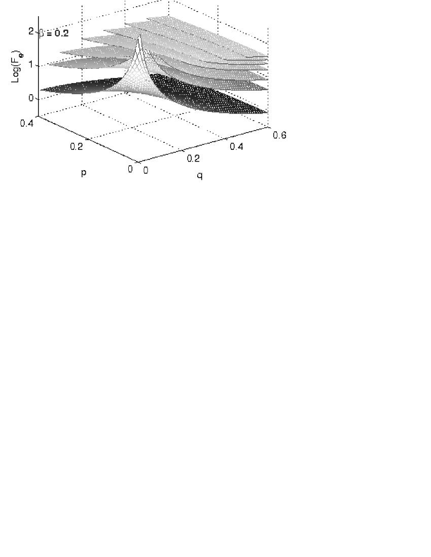
Figure 3: $\log_{10}F_{e}$ for $\beta=.2$.

For further details, see text.

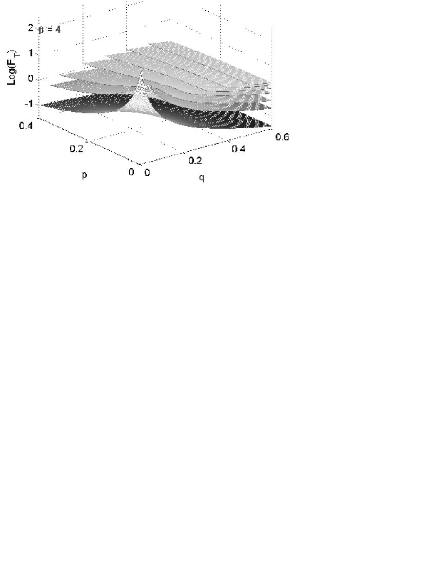
Figure 4: $\log_{10}F_{T}$ for $\beta=4$.

For further details, see text.

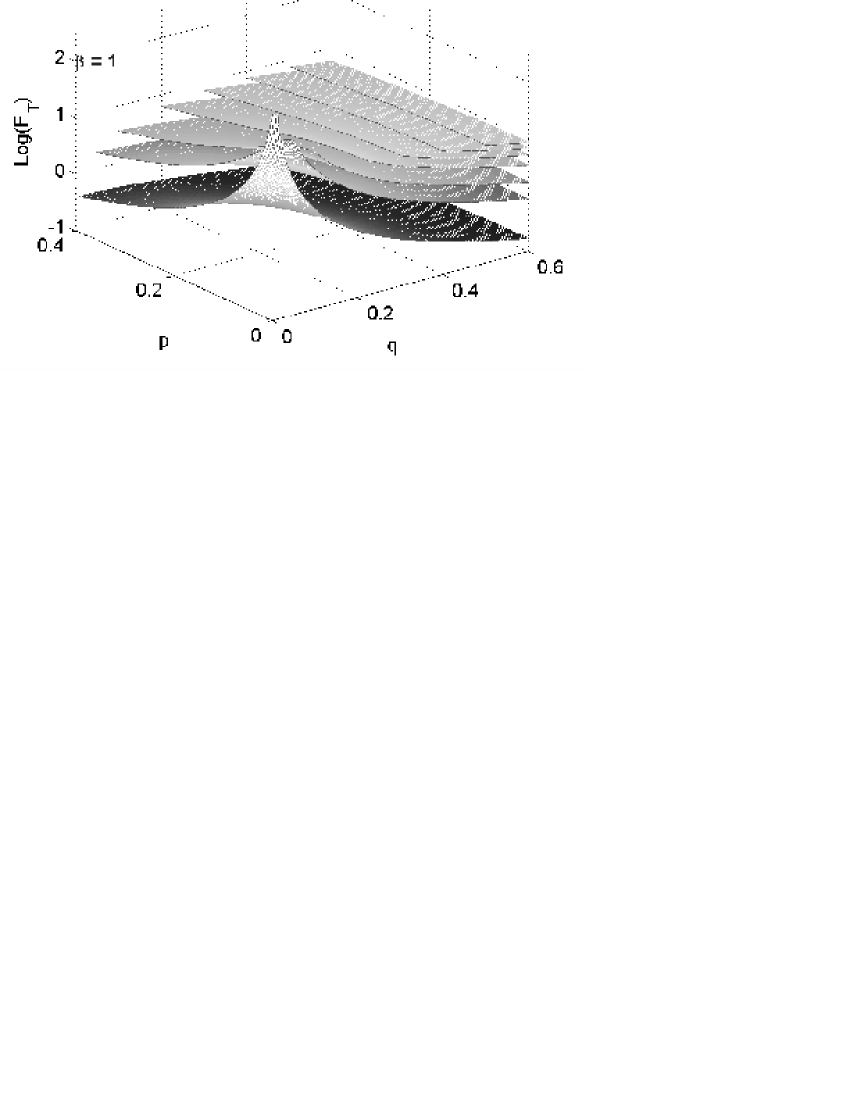
Figure 5: $\log_{10}F_{T}$ for $\beta=1$.

For further details, see text.

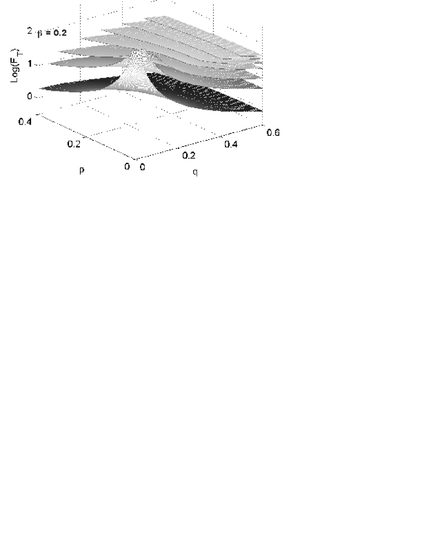
Figure 6: $\log_{10}F_{T}$ for $\beta=.2$.

For further details, see text.

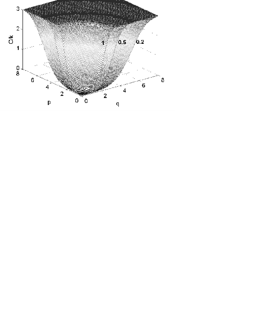
Figure 7: Specific heats for, respectively, $\beta:1,0.5,0,2$ (outwards). For further details, see text.

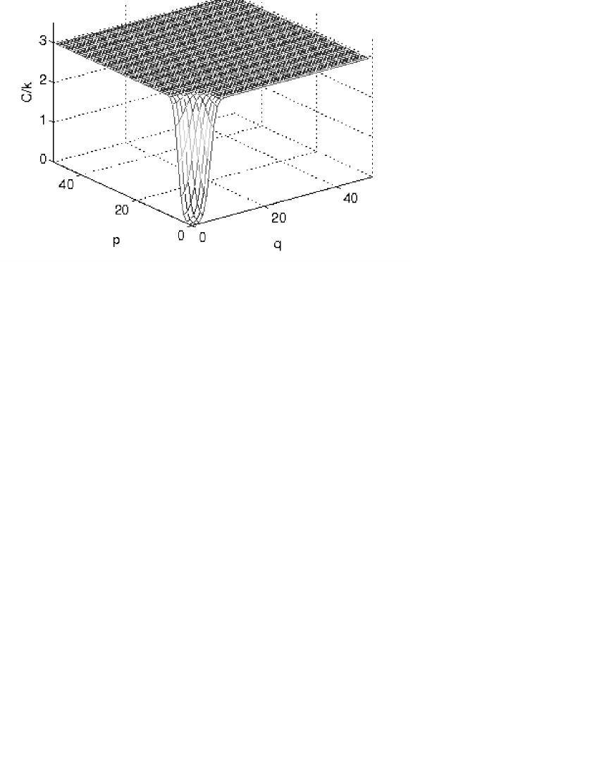
Figure 8: Specific heat for $\beta=0,2$ in an extended $(q,p)$-range For further details, see text.

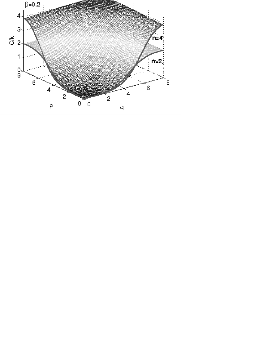
Figure 9: Specific heat for $\beta=0,2$ in an extended $(q,p)$-range in 2 and 4 dimensions. For further details, see text.

References

- [1] M. C. Rocca, A. Plastino, G. L. Ferri, Physica A 393 (2014) 244.
- [2] H. W. de Haan and G. W. Slater, Phys. Rev. E 87, 042604 (2013).
- [3] M. F. Maghrebi, Y. Kantor, and M. Kardar, Phys. Rev. E 86, 061801 (2012).
- [4] E. Verlinde, arXiv:1001.0785 [hep-th]; JHEP 04, 29 (2011).
- [5] A. D. Wissner-Gross and C. E. Freer, Phys. Rev. Lett. 110, 168702 (2013).
- [6] T. Wang, arXiv 0809.4631; D. di Caprio, J.P. Badiali, M. Holovko, arXiv 1009.5561.
- [7] M. H. P. M. van Putten, Phys. Rev. D 85, 064046 (2012).
- [8] N. Shiba, Phys. Rev. D 83, 065002 (2011).
- [9] R. C. Dewar, Entropy 11, 931 (2009); ArXiv 0005382; R. C. Dewar, A. Maritan, ArXiv 1107.1088.
- [10] R.K. Pathria, Statistical Mechanics (Pergamon Press, Exeter, 1993); F. Reif, Statistical and thermal physics (McGraw-Hill, NY, 1965).
- [11] B. H. Lavenda, Statistical Physics (Wiley, New York, 1991); B. H. Lavenda, Thermodynamics of Extremes (Albion, West Sussex, 1995).
- [12] E. T. Jaynes, Phys. Rev. 106, 620 (1957); 108, 171 (1957); Papers on probability, statistics and statistical physics, edited by R. D. Rosenkrantz (Reidel, Dordrecht, Boston, 1987); A. Katz, Principles of Statistical Mechanics, The Information Theory Approach (Freeman and Co., San Francisco, 1967).
- [13] I. S. Gradshteyn and I. M. Ryzhik: “Table of Integrals Series and Products”, 3.191,1, page 284. Academic Press, 1965.
- [14] I. S. Gradshteyn and I. M. Ryzhik: “Table of Integrals Series and Products”, 3.351,3, page 310. Academic Press, 1965.
- [15] I. S. Gradshteyn and I. M. Ryzhik: “Table of Integrals Series and Products”, 3.351,1, page 310. Academic Press, 1965.
- [16] E. A. Deslogue, Thermal Physics (Holt, Rhinehart, and Winston, NY, 1968, p. 37).
- [17] J. Binney and S. Tremaine, Galactic Dynamics (Princeton University Press, Princeton, NJ, 1987).
- [18] P. J. Peebles and B. Bharat, Rev. Mod. Phys. 75 (2003) 559; and references therein.
- [19] P. Sadhukhan and S. M. Bhattacharjee, J. Phys. A 45 (2012) 425302; EuroPhys. Letts. 98 (2012) 10008.