Resonance effects in pion and kaon decay constants

Abstract

In this article we study impact of the lightest vector and scalar resonance multiplets in the pion and kaon decay constants up to next-to-leading order in the $1/N_{C}$ expansion, i.e., up to the one-loop level. The $F_{\pi}$ and $F_{K}$ predictions obtained within the framework of Resonance Chiral Theory are confronted with lattice simulation data. The vector loops (and the $\rho-\pi\pi$ coupling $G_{V}$ in particular) are found to play a crucial role in the determination of the Chiral Perturbation Theory couplings $L_{4}$ and $L_{5}$ at next-to-leading order in $1/N_{C}$. Puzzling, values of $G_{V}\mathrel{\hbox to0.0pt{\lower 4.0pt\hbox{\hskip 1.0pt$\sim$}\hss}\raise 1.0pt\hbox{$<$}}40$ MeV seem to be necessary to agree with current phenomenological results for $L_{4}$ and $L_{5}$. Conversely, a value of $G_{V}\mathrel{\hbox to0.0pt{\lower 4.0pt\hbox{\hskip 1.0pt$\sim$}\hss}\raise 1.0pt\hbox{$>$}}60$ MeV compatible with standard $\rho-\pi\pi$ determinations turns these chiral couplings negative. However, in spite of the strong anti-correlation with $L_{4}$, the $SU(3)$ chiral coupling $F_{0}$ remains stable all the time and stays within the range $78\sim 86$ MeV when $G_{V}$ is varied in a wide range, from $40$ up to $70$ MeV. Finally, we would like to remark that the leading order expressions used in this article for the $\eta-\eta^{\prime}$ mixing, mass splitting of the vector multiplet masses and the quark mass dependence of the $\rho(770)$ mass are found in reasonable agreement with the lattice data.

I Introduction

The decay constants of the light pseudo Nambu-Goldstone bosons (pNGB) $\pi$ and $K$ are important quantities in particle physics. Their precise determinations are crucial for the extraction of the Cabibbo-Kobayashi-Maskawa matrix elements $V_{ud}$ and $V_{us}$ and for beyond Standard Model physics searches in the flavour sector FLAG:2013 ; Bernard:2006 . They are one of the fundamental parameters in chiral perturbation theory ($\chi$PT), the effective field theory (EFT) of Quantum Chromodynamics (QCD) that describes the low-energy interactions between the pNGB ($\pi,K,\eta$) from the spontaneous chiral symmetry breaking Weinberg:1979 ; gl845 . In fact, these two decay constants $F_{\pi}$ and $F_{K}$ have been widely studied in $\chi$PT phenomenology gl845 ; Bijnens:2011tb and lattice simulations FLAG:2013 ; Colangelo:2010et . However due to the rapid proliferation of the number of unknown low energy constants (LECs) at ${\cal O}(p^{6})$, it is rather difficult to extract definitive conclusion on the values of ${\cal O}(p^{4})$ LECs and the ${\cal O}(p^{2})$ coupling $F_{0}$ Bijnens:2011tb ; FLAG:2013 .

In spite of important progresses in the last years, lattice simulations usually compute the pNGB decay constants for values of the quark masses $m_{q}$ heavier than the physical ones, in order to optimize computer resources. This worsens the convergence of the $\chi$PT series and higher chiral orders must be accounted and resummed in an appropriate way. However, apart from the chiral log behaviour at small quark masses, these observables show an almost linear dependence on $m_{q}$, without any significant logarithmic behaviour that one would expect from hadronic loop contributions. The inclusion of resonances within a chiral invariant framework, Resonance Chiral Theory (R$\chi$T) rcht89 , is expected to extend the applicability energy region of $\chi$PT up to some higher scale and explain this feature. The $1/N_{C}$ expansion Nc , with $N_{C}$ the numbers of colors in QCD, is taken as a guiding principle in R$\chi$T to sort out the various contributions, being hadronic loops suppressed by $1/N_{C}$. Indeed, at leading order (LO) in $1/N_{C}$, R$\chi$T predicts an almost linear $m_{q}$ dependence for the decay constants with a slope given by the lightest scalar resonance mass SanzCillero:2004sk , with fit value $M_{S}=1049\pm 25$ MeV: the same scalar resonance that mediates the scalar form-factor into two pNGB at tree-level also rules the quark mass corrections in the weak pNGB decay through an axial-vector current.

In the present work, we calculate the pion and kaon decay constants up to next-to-leading order (NLO) in $1/N_{C}$ within R$\chi$T, i.e., up to the one-loop level, continuing a series of previous NLO computations in this work-line SanzCillero:2009ap ; Rosell-L8 ; Rosell-L9-L10 ; L9a ; Cata:2001nz . We hope in this way to properly incorporate the small $m_{q}$ chiral log behaviour without spoiling the roughly linear dependence found at large $N_{C}$ SanzCillero:2004sk . This will allow us to match $SU(3)$ $\chi$PT at ${\cal O}(p^{4})$ recovering the right renormalization scale dependence of the relevant LECs, $L_{4}(\mu)$ and $L_{5}(\mu)$. These theoretical predictions from R$\chi$T will be then confronted with the lattice results for $F_{\pi}$, $F_{K}$ Davies:2003fw ; Davies:2003ik ; Aoki:2010dy ; Arthur:2012opa and $F_{K}/F_{\pi}$ Durr:2010hr .

The impact of meson resonances on the pNGB decay constants have not been thoroughly discussed in previous literature. The only other one-loop attempt was carried out in the $SU(2)$ case and incorporated only the lightest scalar Soto:2011ap . In this work we discuss the $SU(3)$ chiral dynamics and the effect of vector loops, in addition to the scalar ones. The outcomes in the present article are not expected to provide an improved version of the already very precise $\chi$PT computations present in the market, which are known now up to next-to-next-to-leading order (NNLO) in the chiral expansion FP-Op6 ; Ecker:2013pba and incorporate specific lattice simulation subtleties (twisted boundary conditions lattice-TBC , finite volume effects finite-volume , etc.). The central aim of this article is to show how it is possible to study the dynamics of the lightest resonances through the analysis of these observables in the lattice. In particular we will see that the vector resonance loops (and more precisely the $\rho-\pi\pi$ coupling $G_{V}$) play an important role in the analysis and will be crucial for the final values of the $\chi$PT LECs $F_{0}$, $L_{4}$ and $L_{5}$.

The article is organized as follows: in Sec. II we introduce theoretical setup and the LO and NLO R$\chi$T Lagrangian. In Sec. III we perform the NLO computation in R$\chi$T, renormalization and matching between R$\chi$T and $\chi$PT. The fit to lattice data and the phenomenological discussions are carried out in Sec. IV. We finally provide the conclusions in Sec. V, relegating the most technical details to the Appendices.

II Relevant R$\chi$T Lagrangian

II.1 R$\chi$T building blocks

We will use the exponential realization of the $U(3)_{L}\otimes U(3)_{R}/U(3)_{V}$ coset coordinates for the pNGB,

$$U = u^{2}=e^{i\frac{\sqrt{2}\phi}{F_{0}}}\,,\qquad\qquad D_{\mu}U=\partial_{\mu}U-ir_{\mu}U+iU\ell_{\mu}\,,$$ (1)

where the covariant derivative $D_{\mu}U$ incorporates the right and left external sources, respectively, $r_{\mu}$ and $\ell_{\mu}$, in such a way that it transforms in the same way as $U$ under local chiral transformations gl845 :

$$U\quad\longrightarrow\quad g_{R}\,U\,g_{L}^{\dagger}\,,\qquad\qquad\qquad u\quad\longrightarrow\quad g_{R}\,u\,h^{\dagger}\,\,\,=\,\,\,h\,u\,g_{L}^{\dagger}\,,$$ (2)

with the compensating transformation $h(\phi,g_{R},g_{L})$ rcht89 . Thus, the covariant derivative in Eq. (1) transforms in the form $(D_{\mu}U)\longrightarrow g_{R}\,(D_{\mu}U)\,g_{L}^{\dagger}$.

The pNGB octet plus the singlet $\eta_{1}$ are given by the matrix,

$$\phi\,\,\,=\,\,\,\sum_{a=0}^{8}\phi^{a}\frac{\displaystyle\lambda^{a}}{\displaystyle\sqrt{2}}\,\,\,=\,\,\,\left(\begin{array}[]{ccc}\frac{1}{\sqrt{2}}\pi^{0}+\frac{1}{\sqrt{6}}\eta_{8}+\frac{1}{\sqrt{3}}\eta_{1}&\pi^{+}&K^{+}\\ \pi^{-}&\frac{-1}{\sqrt{2}}\pi^{0}+\frac{1}{\sqrt{6}}\eta_{8}+\frac{1}{\sqrt{3}}\eta_{1}&K^{0}\\ K^{-}&\bar{K}^{0}&\frac{-2}{\sqrt{6}}\eta_{8}+\frac{1}{\sqrt{3}}\eta_{1}\end{array}\right)\,.$$ (3)

Notice that due to the inclusion of the singlet $\eta_{1}$, the standard chiral counting from $SU(3)$–$\chi$PT given by an expansion in powers of the momenta and the pNGB masses does not work any more, since the mass of $\eta_{1}$ does not vanish in the chiral limit ($m_{\eta_{1}}\to M_{0}\simeq 850$ MeV when $m_{q}\to 0$ Feldmann:1999uf ). However, by introducing $1/N_{C}$ as a third expansion parameter, it is still possible to establish a consistent power counting system for $U(3)$–$\chi$PT Kaiser:2000gs , which includes the singlet $\eta_{1}$ as a dynamical degree of freedom (d.o.f).

The basic building blocks of the meson theory read

$$u_{\mu}=iu^{\dagger}D_{\mu}Uu^{\dagger}\,=\,i\{u^{\dagger}(\partial_{\mu}-ir_{\mu})u\,-\,u(\partial_{\mu}-u\ell_{\mu})u^{\dagger}\}\,,$$

$$\chi_{\pm}=u^{\dagger}\chi u^{\dagger}\pm u\chi^{\dagger}u\,,\qquad\qquad f_{\pm}^{\mu\nu}=uF_{L}^{\mu\nu}u^{\dagger}\,\pm\,u^{\dagger}F_{R}^{\mu\nu}u\,,$$ (4)

where $\chi=2B(s+ip)$ includes the scalar ($s$) and pseudo-scalar ($p$) external sources, and $F_{L}^{\mu\nu}$ and $F_{R}^{\mu\nu}$ are, respectively, the left and right field-strength tensors gl845 . All the referred tensors $X=u_{\mu},\,\chi_{\pm},\,f_{\pm}^{\mu\nu}$ transform under chiral transformations as

$$X\quad\longrightarrow\quad h\,X\,h^{\dagger}\,.$$ (5)

We will also make use of the covariant derivative for this type of objects,

$$\nabla_{\mu}X = \partial_{\mu}X+[\Gamma_{\mu},X]\,,\qquad\qquad\Gamma_{\mu}=\frac{1}{2}\bigg{[}u^{\dagger}(\partial_{\mu}-i\,r_{\mu})u+u(\partial_{\mu}-i\,\ell_{\mu})u^{\dagger}\bigg{]}\,.$$ (6)

In our analysis we will study the impact of the lightest $U(3)$ nonets of vector and scalar resonances surviving at large $N_{C}$. We will employ a representation of the resonance fields $R=V,\,S$ such that they transform in the way $R\longrightarrow h\,R\,h^{\dagger}$ in Eq. (5) under chiral transformations rcht89 . The flavor assignment for the scalar and vector resonances is similar to that in Eq. (3):

$$S = \left(\begin{array}[]{ccc}\frac{a_{0}^{0}}{\sqrt{2}}+\frac{\sigma_{8}}{\sqrt{6}}+\frac{\sigma_{1}}{\sqrt{3}}&a_{0}^{+}&\kappa^{+}\\ a_{0}^{-}&-\frac{a_{0}^{0}}{\sqrt{2}}+\frac{\sigma_{8}}{\sqrt{6}}+\frac{\sigma_{1}}{\sqrt{3}}&\kappa^{0}\\ \kappa^{-}&\bar{\kappa}^{0}&-\frac{2\sigma_{8}}{\sqrt{6}}+\frac{\sigma_{1}}{\sqrt{3}}\\ \end{array}\right)\,,$$ (10)

$$V_{\mu\nu} = \left(\begin{array}[]{ccc}\frac{\rho_{0}}{\sqrt{2}}+\frac{1}{\sqrt{6}}\omega_{8}+\frac{1}{\sqrt{3}}\omega_{1}&\rho^{+}&K^{*+}\\ \rho^{-}&-\frac{\rho_{0}}{\sqrt{2}}+\frac{1}{\sqrt{6}}\omega_{8}+\frac{1}{\sqrt{3}}\omega_{1}&K^{*0}\\ K^{*-}&\bar{K}^{*0}&-\frac{2}{\sqrt{6}}\omega_{8}+\frac{1}{\sqrt{3}}\omega_{1}\\ \end{array}\right)_{\mu\nu}\,.$$ (14)

The vector resonances are described here in the antisymmetric tensor formalism through the $V_{\mu\nu}$ fields rcht89 . In later discussions, we will consider the ideal $I=0$ resonance mixings

$$\sigma_{8}=\sqrt{\frac{1}{3}}\sigma-\sqrt{\frac{2}{3}}\sigma^{\prime}\,,\quad\sigma_{1}=\sqrt{\frac{2}{3}}\sigma+\sqrt{\frac{1}{3}}\sigma^{\prime}\,,$$ (15)

$$\omega_{8}=\sqrt{\frac{2}{3}}\phi+\sqrt{\frac{1}{3}}\omega\,,\quad\omega_{1}=\sqrt{\frac{2}{3}}\omega-\sqrt{\frac{1}{3}}\phi\,,$$ (16)

for the octet and singlet scalar and vector resonances, which leads to two different types of isoscalar resonances $R^{\bar{u}u+\bar{d}d}_{I=0}$ and $R^{\bar{s}s}_{I=0}$ in the quark flavour basis. This pattern was found to provide an excellent phenomenological description for the vector resonance multiplets Guo:2009hi . We would like to stress that the resonances incorporated in our framework are the ones surviving at large $N_{C}$. The lowest multiplet of vector resonances ($\rho,K^{*},\omega,\phi$) behaves very approximately like a standard $\bar{q}q$ resonance, with a mass that tends to a constant and a width decreasing like $1/N_{C}$ when $N_{C}\to\infty$ RuizdeElvira:2010cs ; Guo:2011pa ; Guo:2012ym ; Guo:2012yt . This allows us to build a one-to-one correspondence between the physical vector resonances and those surviving at large $N_{C}$. On the other hand, the nature of the light scalar resonances, such as $f_{0}(500)$,$f_{0}(980)$, $K^{*}_{0}(800)$, etc., is still unclear and various descriptions are proposed by different groups: meson-meson molecular, tetraquark, standard $\bar{q}q$ with a strong pion cloud, etc. As a result of this, their $N_{C}$ behavior is also under debate Guo:2011pa ; Guo:2012yt ; RuizdeElvira:2010cs ; Dai:2011bs ; Dai:2012kf ; Zhou:2010ra . Though the $N_{C}$ trajectories of the scalar resonances reported by different groups diverge from each other, surprisingly there is one common feature from Refs. Guo:2011pa ; Guo:2012yt ; RuizdeElvira:2010cs ; Dai:2011bs ; Dai:2012kf : a scalar resonance with mass around 1 GeV appears at large $N_{C}$. Based on these results and the success of this hypothesis in previous analyses Guo:2009hi ; Rosell-L8 ; SanzCillero:2009ap , we will assume in the present article the existence of a large–$N_{C}$ scalar nonet with a bare mass around 1 GeV.

On the other hand, the situation is slightly more cumbersome for $\eta_{8}$ and $\eta_{1}$ and one needs to consider the mixing

$$\eta_{8}=c_{\theta}\eta+s_{\theta}\eta^{\prime}\,,\quad\eta_{1}=-s_{\theta}\eta+c_{\theta}\eta^{\prime}\,,$$ (17)

with $c_{\theta}=\cos{\theta}$ and $s_{\theta}=\sin{\theta}$. Phenomenologically, one has $\theta=(-13.3\pm 0.5)^{\circ}$ in QCD theta-exp , far away from the ideal mixing $\theta=-\arcsin{\sqrt{\frac{2}{3}}}\simeq-55^{\circ}$. We will see that only the leading order mixing will be relevant in the present analysis of $F_{\pi}$ and $F_{K}$.  In the loop calculation, it is convenient to use the physical states $\eta$ and $\eta^{\prime}$, instead of the flavour eigenstates $\eta_{1}$ and $\eta_{8}$. The reason is that the mixing between $\eta_{1}$ and $\eta_{8}$ is proportional to $m_{K}^{2}-m_{\pi}^{2}$, which is formally the same order as the masses of $\eta_{1}$ and $\eta_{8}$. The insertion of the $\eta_{1}$ and $\eta_{8}$ mixing in the chiral loops will not increase the $1/N_{C}$ order of the loop diagrams. This makes the loop calculation technically complicated. However, as already noticed in Refs. Guo:2011pa ; Guo:2012ym ; Guo:2012yt , one can easily avoid the complication in the loop computation by expressing the Lagrangian in terms of the $\eta$ and $\eta^{\prime}$ states resulting from the diagonalization of $\eta_{1}$ and $\eta_{8}$ at leading order. In addition, the effect of the mixing is less and less important in the lattice simulations as $m_{\pi}$ increases and approaches $m_{K}$, making subleading uncertainties in the mixing even more suppressed. Therefore, in the following discussion, we will always calculate the loop diagrams in terms of $\eta$ and $\eta^{\prime}$ states, instead of $\eta_{1}$ and $\eta_{8}$. Further details on the $\eta$–$\eta^{\prime}$ mixing are relegated to App. B.

II.2 LO Lagrangian

In general, one can classify the R$\chi$T operators in the Lagrangian according to the number of resonance fields in the form

$$\mathcal{L}_{R\chi T} = \mathcal{L}_{G}\quad+\quad\sum_{R}\mathcal{L}_{R}\quad+\quad...$$ (18)

where the operators in $\mathcal{L}_{G}$ only contains pNGB and external sources, the $\mathcal{L}_{R}$ terms have one resonance field in addition to possible pNGB and external auxiliary fields, and the dots stand for operators with two or more resonances.

We focus first on the $\mathcal{L}_{G}$ part of the R$\chi$T Lagrangian. Since we will later incorporate the lightest $U(3)$ nonet of hadronic resonances and we are working within a large–$N_{C}$ framework, our theory will be based on the $U(3)_{L}\otimes U(3)_{R}$ symmetry and, in addition to the two usual ${\cal O}(p^{2})$ operators from $SU(3)$ $\chi$PT, we will also need to consider the singlet $\eta_{1}$ mass term:

$$\mathcal{L}_{G}^{\rm LO}\,\,\,=\,\,\,\frac{\widetilde{F}^{2}}{4}\langle u_{\mu}u^{\mu}\rangle\,+\frac{\hat{F}^{2}}{4}\langle\chi_{+}\rangle+\frac{F_{0}^{2}}{3}M_{0}^{2}\ln^{2}{\det u}\,,$$ (19)

where $\langle\ldots\rangle$ stands for the trace in flavor space. The last operator in the right-hand side (r.h.s.) of Eq. (19) is generated by the $U_{A}(1)$ anomaly and gives mass to the singlet $\eta_{1}$. On the contrary to $\chi$PT, in R$\chi$T one generates ultraviolet (UV) divergences which require the first two terms in the r.h.s of Eq. (19) to fulfill the renormalization of the resonance loops SanzCillero:2009ap ; RChT-gen-fun . Notice that a different coupling notation $\alpha_{1}=\widetilde{F}^{2}/4$ and $\alpha_{2}=\hat{F}^{2}/4$ is used in Ref. RChT-gen-fun . As $\widetilde{F}$ and $\hat{F}$ describe the chiral limit pNGB decay constant from an axial-vector current and a pseudo-scalar density, respectively, one has that $\lim_{N_{C}\to\infty}\widetilde{F}/F_{0}=\lim_{N_{C}\to\infty}\hat{F}/F_{0}=1$. $F_{0}$ stands for the $n_{f}=3$ decay constant of the pNGB octet in the chiral limit. The parameter $B$ in $\chi_{+}$ from Eq. (II.1) is connected with the quark condensate through $\langle 0|\bar{q}^{i}q^{j}|0\rangle=-F_{0}^{2}B\delta^{ij}$ in the same limit. The explicit chiral symmetry breaking is realized by setting the scalar external source field to $s={\rm Diag}(m_{u},m_{d},m_{s})$, being $m_{q}$ the light quark masses. We will consider the isospin limit all along the work, i.e., we will take $m_{u}=m_{d}$ (denoted just as $m_{u/d}$) and neglect any electromagnetic correction.

In order to account for the resonance effects, we consider the minimal resonance operators in the leading order R$\chi$T Lagrangian rcht89

$$\mathcal{L}_{V} = \frac{F_{V}}{2\sqrt{2}}\langle V_{\mu\nu}f_{+}^{\mu\nu}\rangle+\frac{iG_{V}}{2\sqrt{2}}\langle V_{\mu\nu}[u^{\mu},u^{\nu}]\rangle\,,$$ (20)

$$\mathcal{L}_{S} = c_{d}\langle\,Su_{\mu}u^{\mu}\,\rangle+c_{m}\langle\,S\chi_{+}\,\rangle\,.$$ (21)

In general, one could consider the resonance operators of the type $\langle\,R\chi^{(n\geq 4)}(\phi)\,\rangle$, with the chiral tensor $\chi^{{(n)}}(\phi)$ only including the pNGB and external fields and $n$ standing for the chiral order of this chiral tensor. The resonance operators in the previous two equations are of type $\langle\,R\chi^{(2)}(\phi)\,\rangle$. Operators with higher values of $n$ tend to violate the high-energy asymptotic behaviour dictated by QCD for form-factors and Green functions. Likewise, by means of meson field redefinitions it is possible to trade some resonance operators by other terms with a lower number of derivatives and operators without resonance fields RChT-RGE ; SanzCillero:2009ap ; L9a ; EoM . As a result of this, only the lowest order chiral tensors are typically employed to build the operators of the leading order R$\chi$T Lagrangian. We will follow this heuristic rule in the present work. Nevertheless, we remind the reader that the truncation of the infinite tower of large-$N_{C}$ resonances introduces in general a theoretical uncertainty in the determinations, which will be neglected in our computation. Considering only the lightest resonance multiplets may lead to some issues with the short-distance constraints and the low-energy predictions when a broader and broader set of observables is analyzed truncation .

In Ref. Guo:2011pa , two additional resonance operators were taken into account (last two terms in Eq. (5) of the previous reference). These two terms are $1/N_{C}$ suppressed with respect to the R$\chi$T operator in Eq. (21). They happen to be irrelevant for our current study up to NLO in $1/N_{C}$ since they involve at least one $\eta$ or $\eta^{\prime}$ fields. As we already mentioned previously, $\eta$ and $\eta^{\prime}$ only enter our calculation through chiral loops and the two additional operators in Ref. Guo:2011pa would contribute to $F_{\pi}$ and $F_{K}$ at next-to-next-to-leading order in $1/N_{C}$. Thus, the one-loop calculation at NLO in $1/N_{C}$ only requires the consideration of the LO resonance operators like those in Eqs. (20) and (21).

The corresponding kinematical terms for resonance fields are rcht89

$$\mathcal{L}_{\rm kin}^{V} = -{1\over 2}\langle\,\nabla^{\lambda}V_{\lambda\mu}\nabla_{\nu}V^{\nu\mu}-{1\over 2}\overline{M}^{2}_{V}V_{\mu\nu}V^{\mu\nu}\,\rangle\,,$$ (22)

$$\mathcal{L}_{\rm kin}^{S} = {1\over 2}\langle\,\nabla^{\mu}S\nabla_{\mu}S-\overline{M}^{2}_{S}S^{2}\,\rangle\,.$$ (23)

In our current work, we also incorporate the light quark mass corrections to the resonance masses and in the large $N_{C}$ limit this effect is governed by the operators MR-split  

$$\mathcal{L}_{RR}^{\rm split} = e_{m}^{S}\langle\,SS\chi_{+}\,\rangle\,\,\,-\,\,\,\frac{\displaystyle 1}{\displaystyle 2}\,e_{m}^{V}\langle\,V_{\mu\nu}V^{\mu\nu}\chi_{+}\,\rangle\,.$$ (24)

In the notation of Ref. Op6-RChT these two couplings would be given by $e_{m}^{S}=\lambda_{3}^{SS}$ and $e_{m}^{V}=-2\lambda_{6}^{VV}$. If no further bilinear resonance term is included in the Lagrangian, one has an ideal mixing for the two $I=0$ resonances in the nonet and a mass splitting pattern of the form

$$(M^{\bar{u}u+\bar{d}d}_{I=0})^{2}=M^{2}_{I=1} = \overline{M}_{R}^{\,\,2}-4e_{m}^{R}m_{\pi}^{2}\,,$$

$$M^{2}_{I=\frac{1}{2}} = \overline{M}_{R}^{\,\,2}-4e_{m}^{R}m_{K}^{2}\,\,\,\,,$$

$$M^{(\bar{s}s)\,\,\,2}_{I=0} = \overline{M}_{R}^{\,\,2}-4e_{m}^{R}\,\,(2m_{K}^{2}-m_{\pi}^{2})\,\,\,\,,$$ (25)

with $\overline{M}_{R}$ the resonance mass in chiral limit. Notice that in the following we will use the notations $M_{S}$ and $M_{V}$ for the masses of scalar and vector multiplets in chiral limit, respectively.

At large $N_{C}$, the coupling of the LO Lagrangian scale like $F_{0},\,\widetilde{F},\,\hat{F},\,G_{V},\,c_{d},\,c_{m}=\,{\cal O}(N_{C}^{\frac{1}{2}})$ and the masses of the mesons considered here behave like $m_{\phi},\,M_{R},\,=\,{\cal O}(N_{C}^{0})$, with the splitting parameter $e_{m}^{R}\,=\,{\cal O}(N_{C}^{0})$. The $\eta_{1}$ mass chiral limit $M_{0}$ is formally ${\cal O}(N_{C}^{-1})$, although numerically provides a sizable contribution to the $\eta-\eta^{\prime}$ mixing that needs to be taken into account in order to properly reproduce their masses and mixing angles. More details can be found in App. B.

II.3 NLO R$\chi$T Lagrangian

In general, one should also take into account local operators with a higher number of derivatives (e.g. ${\cal O}(p^{4})$) in R$\chi$T. In particular one might consider operators composed only of pNGB and external fields. Notice that these terms of the R$\chi$T Lagrangian are different from those in $\chi$PT, as they are two different quantum field theories with different particle content.

Based on phenomenological analyses and short-distance constraints it is well known that the leading parts of the $\chi$PT LECs are found to be saturated by the lowest resonances at large $N_{C}$ rcht89 ; SD-RChT . The operators of R$\chi$T without resonances of ${\cal O}(p^{d\geq 4})$ can be regarded as $1/N_{C}$ suppressed residues, absent when $N_{C}\to\infty$. Nonetheless the resonance saturation scale cannot be determined at large $N_{C}$ as this is a NLO effect in $1/N_{C}$. Since in this work we perform the discussion at the NLO of $1/N_{C}$, we will include these residual R$\chi$T operators without resonance fields, which start being relevant at NLO in $1/N_{C}$.

The pertinent ${\cal O}(p^{4})$ operators in our study are gl845

$$\mathcal{L}_{G}^{\rm NLO} = \widetilde{L}_{4}\langle\,u_{\mu}u^{\mu}\,\rangle\langle\,\chi_{+}\,\rangle+\widetilde{L}_{5}\langle\,u_{\mu}u^{\mu}\chi_{+}\,\rangle+\widetilde{L}_{6}\langle\,\chi_{+}\,\rangle\langle\,\chi_{+}\,\rangle+\widetilde{L}_{7}\langle\,\chi_{-}\,\rangle\langle\,\chi_{-}\,\rangle$$ (26)

$$+\frac{\widetilde{L}_{8}}{2}\langle\,\chi_{+}\chi_{+}+\chi_{-}\chi_{-}\,\rangle+i\,\widetilde{L}_{11}\langle\,\chi_{-}\big{(}\nabla_{\mu}u^{\mu}-\frac{i}{2}\chi_{-}+\frac{i}{2{n_{f}}}\langle\,\chi_{-}\,\rangle\big{)}\,\rangle$$

$$-\widetilde{L}_{12}\langle\,\big{(}\nabla_{\mu}u^{\mu}-\frac{i}{2}\chi_{-}+\frac{i}{2{n_{f}}}\langle\,\chi_{-}\,\rangle\big{)}^{2}\,\rangle\,,$$

where $n_{f}=3$ and the tilde is introduced to distinguish the R$\chi$T couplings from the $\chi$PT LECs $L_{j}$. The set of $\mathcal{L}_{G}^{\rm NLO}$ couplings scale like $\widetilde{L}_{j}\,=\,{\cal O}(N_{C}^{0})$ within the $1/N_{C}$ expansion and are suppressed with respect to the ${\cal O}(p^{4})$ LECs, which behave like $L_{j}\,=\,{\cal O}(N_{C})$. The parameters $\widetilde{L}_{11}$ and $\widetilde{L}_{12}$ will not appear in the final results for $F_{\pi}$ and $F_{K}$, as their contributions in the matrix element of the axial-vector current will be canceled out by the wave function renormalization constant of the pNGB.

One should notice that the chiral operators in the previous equation are exactly the same as in $\chi$PT, but the coefficients can be completely different. In order to extract the low-energy EFT couplings one needs to integrate out the heavy d.o.f in the R$\chi$T action. At tree-level, the $\chi$PT LECs get two kinds of contributions: one comes directly from the $\widetilde{L}_{i}$ operators with only pNGB and external sources; the other, $L_{i}^{\rm Res}$, comes from the tree-level resonance exchanges when $p^{2}\ll M_{R}^{2}$. Hence, the relations between the couplings in R$\chi$T and those in $\chi$PT are given by rcht89 ; SD-RChT ; NLO-saturation

$$L_{i}^{\chi{\rm PT}}=L_{i}^{{\rm Res}}+\widetilde{L}_{i}\,.$$ (27)

From now on, in order to avoid any possible confusion we will explicitly write the superscript $\chi$PT when referring the chiral LECs. The large–$N_{C}$ resonance contributions to the ${\cal O}(p^{4})$ LECs were computed in Ref. rcht89 by integrating out the resonance in the R$\chi$T generating functional, yielding

$$\left.L_{4}^{{\rm Res}}\right|_{N_{C}\to\infty}\,=\,0\,,\qquad\qquad\left.L_{5}^{{\rm Res}}\right|_{N_{C}\to\infty}\,=\,\left.\frac{c_{d}c_{m}}{M_{S}^{2}}\right|_{N_{C}\to\infty}\,=\,\frac{\displaystyle F_{0}^{2}}{\displaystyle 4M_{S}^{2}}\,,$$ (28)

where in the last equality we have used the high-energy scalar form-factor constraint $4c_{d}c_{m}=F_{0}^{2}$ Jamin:2001zq . Other couplings in Eq. (26) will be irrelevant to our final results for the pion and kaon decay constants.

II.4 Scalar resonance tadpole and the field redefinition

Before stepping into the detailed calculation, we point out a subtlety about the treatment of the scalar resonance operators in Eq. (21). The operator with $c_{m}$ coupling in this equation leads to a term that couples the isoscalar scalar resonances $S_{8}$ and $S_{1}$ to the vacuum. In other words, it generates a scalar resonance tadpole proportional to the quark masses. Though it is not a problem to perform the calculations with such tadpole effects, it can be rather cumbersome. We find it is convenient to eliminate it at the Lagrangian level. This will greatly simplify the calculation when the resonances enter the loops. Nonetheless, at tree-level it does not make much difference to eliminate the tadpole at the Lagrangian level SanzCillero:2004sk or just to calculate perturbatively the tadpole diagrams Guo:2011pa ; Guo:2012ym ; Guo:2012yt .

In order to eliminate the scalar tadpole effects from the Lagrangian, we make the following field redefinition for the scalar resonances

$$S=\overline{S}+\frac{c_{m}}{M_{S}^{2}}\chi_{+}\,,$$ (29)

with $\overline{S}$ being the scalar resonance fields after the field redefinition. By substituting Eq. (29) into Eqs.(21) and (23), one has

$$\mathcal{L}_{\rm kin}^{S}\,+\,\mathcal{L}_{S} = {1\over 2}\langle\,\nabla^{\mu}\overline{S}\nabla_{\mu}\overline{S}-M^{2}_{S}\overline{S}^{2}\,\rangle\,+\,c_{d}\langle\,\overline{S}u_{\mu}u^{\mu}\,\rangle\,+\frac{\displaystyle c_{m}}{\displaystyle M_{S}^{2}}\langle\,\nabla_{\mu}\overline{S}\nabla^{\mu}\chi_{+}\,\rangle$$ (30)

$$\quad+\,\frac{\displaystyle c_{d}c_{m}}{\displaystyle M_{S}^{2}}\langle\,\chi_{+}u_{\mu}u^{\mu}\,\rangle\,+\,\frac{\displaystyle c_{m}^{2}}{\displaystyle 2M_{S}^{2}}\langle\,\chi_{+}\chi_{+}\,\rangle$$

$$\quad\,+\,\frac{\displaystyle c_{m}^{2}}{\displaystyle 2M_{S}^{4}}\langle\,\nabla_{\mu}\chi_{+}\nabla^{\mu}\chi_{+}\,\rangle\,.$$

The first line has the same structure as the original Lagrangian with $S$ replaced by $\overline{S}$ but with the corresponding tadpole operator $c_{m}\langle\,\overline{S}\chi_{+}\,\rangle$ absent. Instead, it has been traded out by the derivative term $\frac{c_{m}}{M_{S}^{2}}\langle\,\nabla_{\mu}\overline{S}\nabla^{\mu}\chi_{+}\,\rangle$ at the price of the extra operators in the second and third lines. We want to note that the last operator in Eq.(30) is not considered in the following discussion, as it corresponds to the set of local ${\cal O}{(p^{6})}$ operators without resonance fields and contributes to the decay constants at the order of $m_{q}^{2}$, which was neglected and discarded in previous section. This kind of contributions escapes the control of the present analysis, as there are many other types of resonance operators (e.g. the previously mentioned $\langle\,S\chi^{(4)}(\phi)\,\rangle$ type) which would generate similar terms without resonances after the scalar field redefinition in Eq. (29) but were neglected here. The same applies to the resonance mass splitting Lagrangian $\mathcal{L}_{RR}^{\rm split}$ in Eq. (24): the scalar field redefinition in Eq. (29) generates extra splitting operators of order $m_{q}^{2}$ and $m_{q}^{3}$ which will be neglected in this work.

At NLO in $1/N_{C}$, the LO Lagrangian (21) induces a scalar resonance tadpole proportional to $m_{q}^{2}$ through a pNGB loop. In order to remove it one should perform another scalar field shift similar to Eq. (29) but of the form $\Delta S\sim\frac{c_{j}m_{\phi}^{4}}{16\pi^{2}F_{0}^{2}M_{S}^{2}}$, with $c_{j}=c_{d},c_{m}$. This yields a contribution to the pNGB decay constants doubly suppressed, by $m_{\phi}^{4}$ and $1/N_{C}$. Hence, following the previous considerations, we will neglect the one-loop tadpole effects.

Hence, after performing the shift in the scalar field worked out in this section, R$\chi$T contains operators without resonances in Eq. (30) with the same structure as the $L_{j}$ ones in the ${\cal O}(p^{4})$ $\chi$PT Lagrangian gl845 . Combining Eqs. (26) and (30), we have the effective couplings in R$\chi$T

$$\widetilde{\widetilde{L_{4}}}\,=\,\widetilde{L_{4}}\,,\qquad\qquad\widetilde{\widetilde{L_{5}}}\,=\,\frac{\displaystyle c_{d}c_{m}}{\displaystyle M_{S}^{2}}+\widetilde{L_{5}}\,,\qquad\qquad\widetilde{\widetilde{L_{8}}}\,=\,\frac{\displaystyle c_{m}^{2}}{\displaystyle 2M_{S}^{2}}+\widetilde{L_{8}}\,,$$ (31)

with the couplings of the remaining ${\cal O}(p^{4})$ operators without resonances just given by $\widetilde{\widetilde{L}}_{j}=\widetilde{L}_{j}$. In general the double-tilde notation will refer to the coupling of the Lagrangian operator after performing the scalar field shift in Eq. (29). It is easy to observe that at large $N_{C}$ one recovers the R$\chi$T results in Eq. (28): $\widetilde{\widetilde{L}}_{4}$ and $\widetilde{\widetilde{L}}_{5}$ become equal to the ${\cal O}(p^{4})$ LECs $L_{4}^{\chi PT}$ and $L_{5}^{\chi PT}$, respectively, as there is no other possible ${\cal O}(p^{4})$ resonance contribution of this kind after performing the $S$–shift in Eq. (29). Though $L_{8}$ will not enter the discussion in the pion and kaon decay constants, for completeness we comment that our result in Eq. (31) is consistent with the scalar contributions in Ref. rcht89 , as $\widetilde{\widetilde{L}}_{8}$ would become equal to $L_{8}^{\chi PT}$ in the large–$N_{C}$ limit.

III Theoretical calculation

III.1 Decay constants in R$\chi$T at NLO in $1/N_{C}$

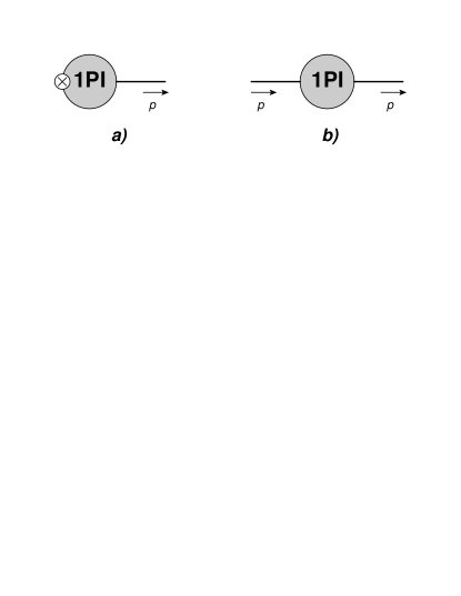
Figure 1: Relevant vertex functions for the physical pNGB decay constant: a) 1PI transitions between an axial-vector current and a bare pseudo-Goldstone field, determining $F_{\phi}^{\rm 1PI}$; b) pNGB self-energy $-i\Sigma_{\phi}(p^{2})$. The solid line stands for a pNGB $\phi$, the crossed circle for an axial-vector current insertion and the circle represents all possible 1PI topologies.

The pNGB decay constant is defined through the matrix element of the axial-vector current of the light quarks

$$\langle\,\phi(p)|\bar{q}\gamma_{\mu}\gamma_{5}u|0\,\rangle=-i\sqrt{2}F_{\phi}p_{\mu}\,,\qquad\qquad\mbox{with }\phi=\pi\,\,(K)\quad\mbox{for }q=d\,\,(s)\,.$$ (32)

In order to study the pion and kaon axial decay constants at NLO of $1/N_{C}$, we need to calculate the one-loop diagrams with resonances running inside the loops and then perform the renormalization. If the scalar tadpole is conveniently cancelled out in the way explained in Sec. II.4, the renormalized matrix element that provides $F_{\phi}$ is then determined by the two 1-Particle-Irreducible (1PI) vertex functions depicted in Fig. 1. More explicitly, we plot in Figs. 2 and 3 the precise diagrams which will be relevant in our R$\chi$T computation of the pNGB decay constant up to NLO of $1/N_{C}$. Hence, the expression for the physical decay constant consist of two pieces

$$F_{\phi}\,\,\,=\,\,\,Z_{\phi}^{\frac{1}{2}}\,\,\,F_{\phi}^{\rm 1PI}\,,$$ (33)

where $Z_{\phi}$ stands for the wave-function renormalization constant of the pNGB given by $\phi^{(B)}=Z_{\phi}^{\frac{1}{2}}\phi^{r}$ ($\phi=\pi,\,K$) in the on-shell scheme (Fig. 1.b) and $F_{\phi}^{\rm 1PI}$ denotes the contributions from 1PI topologies for the transition between an axial-vector current and a bare pNGB $\phi^{(B)}$ (Fig 1.a). The wave-function renormalization constant $Z_{\phi}=1+\delta Z_{\phi}$ is related to the pNGB self-energy $\Sigma_{\phi}(p^{2})$ through

$$Z_{\phi} = \,\,\,\left(\,1\,-\,\Sigma^{\prime}_{\phi}\right)^{-1}\,\,\,=\,\,\,\left(\,1\,-\,\frac{\displaystyle d\Sigma_{\phi}(p^{2})}{\displaystyle dp^{2}}\bigg{|}_{p^{2}=m_{\phi}^{2}}\right)^{-1}\,.$$ (34)

For convenience, we will explicitly separate the tree-level and one-loop contributions in R$\chi$T,

$$Z_{\phi} = \left(\,\frac{\displaystyle\widetilde{F}^{2}}{\displaystyle F_{0}^{2}}\,\,\,+\,\,\,\frac{\displaystyle 8\widetilde{\widetilde{L}}_{4}\,(2m_{K}^{2}+m_{\pi}^{2})}{\displaystyle F_{0}^{2}}\,\,\,+\,\,\,\frac{\displaystyle 8\widetilde{\widetilde{L}}_{5}\,m_{\phi}^{2}}{\displaystyle F_{0}^{2}}\,\,\,+\,\,\,\frac{\displaystyle 8\widetilde{L}_{11}\,m_{\phi}^{2}}{\displaystyle F_{0}^{2}}\,\,\,-\,\,\,\Sigma^{\prime}_{\phi,\,1\ell}\,\right)^{-1}\,,$$ (35)

$$\frac{\displaystyle F_{\phi}^{\rm 1PI}}{\displaystyle F_{0}} = \frac{\displaystyle\widetilde{F}^{2}}{\displaystyle F_{0}^{2}}\,+\,\frac{\displaystyle 8\widetilde{\widetilde{L}}_{4}\,(2m_{K}^{2}+m_{\pi}^{2})}{\displaystyle F_{0}^{2}}\,+\,\frac{\displaystyle 8\widetilde{\widetilde{L}}_{5}\,m_{\phi}^{2}}{\displaystyle F_{0}^{2}}\,\,\,+\,\,\,\frac{\displaystyle 4\widetilde{L}_{11}\,m_{\phi}^{2}}{\displaystyle F_{0}^{2}}\,\,\,+\,\,\,\frac{\displaystyle F^{\rm 1PI}_{\phi,\,1\ell}}{\displaystyle F_{0}}\,,$$ (36)

with the corresponding one-loop corrections $\Sigma^{\prime}_{\phi,\,1\ell}$ and $F^{\rm 1PI}_{\phi,\,1\ell}$. This yields the physical decay constant given by

$$F_{\phi} = \,\,\,F_{0}\,\,\,\bigg{(}\,\,\,\frac{\displaystyle\widetilde{F}}{\displaystyle F_{0}}\,+\,\frac{\displaystyle 4\widetilde{\widetilde{L}}_{4}\,(2m_{K}^{2}+m_{\pi}^{2})}{\displaystyle F_{0}^{2}}\,+\,\frac{\displaystyle 4\widetilde{\widetilde{L}}_{5}\,m_{\phi}^{2}}{\displaystyle F_{0}^{2}}\,\,\,+\,\,\,\frac{\displaystyle F^{\rm 1PI}_{\phi,\,1\ell}}{\displaystyle F_{0}}\,\,\,+\,\,\,\frac{\displaystyle 1}{\displaystyle 2}\Sigma^{\prime}_{\phi,\,1\ell}\,\,\,\bigg{)}\,,$$ (37)

where $Z_{\phi}^{\frac{1}{2}}$ has been expanded in this expression, keeping just the linear contribution in $\delta Z_{\phi}$ and dropping other terms ${\cal O}((\delta Z_{\phi})^{2})$ or higher. In particular, we have used $\widetilde{F}/F_{0}=1+{\cal O}(N_{C}^{-1})$ and dropped terms ${\cal O}\left((\widetilde{F}/F_{0}-1)^{2}\right)$. Notice that there is not a uniquely defined way of truncating the NNLO corrections: for instance, a slightly different numerical prediction is obtained if instead of the expression for $F_{\phi}$ in Eq. (37) one employs the NLO result for $F_{\phi}^{2}$, dropping terms ${\cal O}((\delta Z_{\phi})^{2})$ or higher as we did in Eq. (37). The spurious coupling $\widetilde{L}_{11}$ (corresponding to an operator proportional to the equations of motion SanzCillero:2009ap ) becomes then cancelled out and disappears from the physical observable.

Since we did not consider ${\cal O}(p^{6})$ operators in the Lagrangian $\mathcal{L}_{G}^{\rm LO}$ in Eq. (19), we will neglect the terms ${\cal O}(\widetilde{\widetilde{L}}_{4,5}^{2}m_{\phi}^{4}/F^{4})$ in the decay constant in Eq. (37) which would arise from the expansion at that order of $Z_{\phi}^{\frac{1}{2}}$. In spite of having the same tree-level structure, in general the loop UV–divergences in $Z_{\phi}$ and $F_{\phi}^{\rm 1PI}$, given respectively in Eqs. (35) and (36), are different. Thus, one must combine these two quantities into Eq. (37) in order to get a finite decay constant $F_{\phi}$ by means of the renormalization of $\widetilde{F}$, $\widetilde{\widetilde{L}}_{4}$ and $\widetilde{\widetilde{L}}_{5}$.

In the $N_{C}\to\infty$ limit, the meson loops are absent one has

$$\widetilde{\widetilde{L}}_{4}\,=\,\widetilde{L}_{4}\,,\qquad\qquad\widetilde{\widetilde{L}}_{5}\,\,=\,\left(\widetilde{L}_{5}+\frac{\displaystyle c_{d}c_{m}}{\displaystyle M_{S}^{2}}\right)\,=\,\frac{\displaystyle F_{0}^{2}}{\displaystyle 4M_{S}^{2}}\,,$$ (38)

where we considered the large–$N_{C}$ high-energy constraints $\widetilde{L}_{4}=\widetilde{L}_{5}=0$ and $(4c_{d}c_{m}/F_{0}^{2})=1$ from the scalar form-factor Jamin:2001zq . At LO in $1/N_{C}$ this yields the prediction SanzCillero:2004sk

$$F_{\phi} = \,\,\,F_{0}\,\,\,\bigg{(}\,\,\,1\,\,\,+\,\,\,\frac{\displaystyle 4c_{d}c_{m}}{\displaystyle F_{0}^{2}}\,\frac{\displaystyle m_{\phi}^{2}}{\displaystyle M_{S}^{2}}\,\,\,\bigg{)}\,\,\,=\,\,\,F_{0}\,\,\,\bigg{(}\,\,\,1\,\,\,+\,\,\,\frac{\displaystyle m_{\phi}^{2}}{\displaystyle M_{S}^{2}}\,\,\,\bigg{)}\,,$$ (39)

which reproduce the $F_{\pi}$ and $F_{K}$ lattice data fairly well up to pion masses of the order of 700 MeV SanzCillero:2004sk . The large–$N_{C}$ relation $c_{d}=c_{m}$ Jamin:2001zq was used in Ref. SanzCillero:2004sk to produce Eq. (39), where it led to the relation $m_{\phi}^{2}=B_{0}(m_{q_{1}}+m_{q_{2}})$ between the pNGB mass and the masses of its two valence quarks. We have also used that $\widetilde{F}/F_{0}=1$ and $\Sigma_{\phi,1\ell}=F^{\rm 1PI}_{\phi,1\ell}=0$ when $N_{C}\to\infty$. The only region where this description deviated significantly from the data was in the light pion mass range, where the chiral logs need to be included to properly reproduce the lattice simulation in that regime Davies:2003fw ; Davies:2003ik . Here in Eq. (39) the coupling $F_{0}$ implicitly refers to the $n_{f}=3$ decay constant in that same limit, this is, at large $N_{C}$.

In summary, our calculation of the pNGB decay constants $F_{\phi}$ (with $\phi=\pi,\,K$) is sorted out in the form

$$\frac{\displaystyle F_{\phi}}{\displaystyle F_{0}}\quad = \quad\frac{\displaystyle\Delta F_{\phi}}{\displaystyle F_{0}}\bigg{|}_{{\cal O}(N_{C}^{0})}\quad+\quad\frac{\displaystyle\Delta F_{\phi}}{\displaystyle F_{0}}\bigg{|}_{{\cal O}(N_{C}^{-1})}\quad+\quad...$$ (40)

with the dots standing for terms of ${\cal O}(N_{C}^{-2})$ and higher, which will be neglected in the present article. In the joined large–$N_{C}$ and chiral limits one has the right-hand side becomes equal to one by construction, as $F_{0}=\lim_{m_{u,d,s}\to 0}F_{\phi}$. At large–$N_{C}$, the relevant couplings in the quark mass corrections to $F_{\phi}$ are related with the scalar form-factor and can be fixed through high-energy constraints SanzCillero:2004sk ; Jamin:2001zq . However, one should be aware that it is not possible to have a full control of the quark mass corrections beyond the linear $m_{q}$ term. In fact, including all possible $m_{q}^{2}$ corrections corresponds to considering the full sets of local ${\cal O}(p^{6})$ operators without resonance fields. The complexity of higher order $m_{q}$ corrections not only happens for the NLO in $N_{C}$ but also for the LO case. For instance, large–$N_{C}$ contributions to the scalar (vector) multiplet mass splitting can be in principle of an arbitrary order in $m_{q}$, leading to LO (NLO) corrections in $1/N_{C}$ to $F_{\phi}$ with arbitrary powers of the quark mass. Clearly, there is not a uniquely defined truncation procedure.

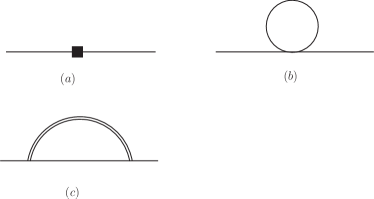
Figure 2: Feynman diagrams of the pNGB self energy. The single line corresponds to pNGB and the double-line stands for a resonance state. The tree level amplitude in diagram (a) can receive contributions both from the leading order Lagrangian in Eq.(19) , the contact terms appearing in the second line of Eq.(30) and the ${\cal O}(p^{4})$ Lagrangian in Eq.(26).

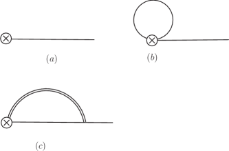
Figure 3: Feynman diagrams of the pNGB axial-vector decay constant. The circled cross symbol corresponds to the axial-vector source. Similar to Fig. 2, diagram (a) can receive contributions from the leading order Lagrangian in Eq.(19), the contact terms appearing in the second line of Eq.(30) and the ${\cal O}(p^{4})$ Lagrangian in Eq.(26).

III.2 Renormalization in R$\chi$T

The calculation of the Feynman diagrams contributing to $F_{\phi}$ up to NLO in $1/N_{C}$ is straightforward (Figs. 2 and 3), though the final results are quite lengthy and have been relegated to App. C for the sake of clarity and in order not to interrupt our discussion. We take into account the $m_{q}$ dependence of the resonance masses in the propagators in the loops, which is given by Eq. (II.2).

In order to have finite results for the physical quantities $F_{\pi}$ and $F_{K}$, the next step consists on performing the renormalization. As in conventional $\chi$PT gl845 we use the dimensional regularization method and the $\rm{\overline{MS}}-1$ renormalization scheme where we will subtract from the Feynman integrals the UV–divergence

$$\frac{1}{\hat{\epsilon}} = \mu^{-2\epsilon}\,\left(\frac{1}{\epsilon}-\gamma_{E}+\ln{4\pi}+1\right)\,\,\,=\,\,\,\frac{1}{\epsilon}-\gamma_{E}+\ln{4\pi}+1-\ln\mu^{2}+{\cal O}(\epsilon)\,,\quad\quad(\epsilon=2-\frac{D}{2})\,.$$

The UV–divergences from loops can be absorbed through a convenient renormalization of the R$\chi$T couplings $C_{\chi}=\widetilde{F},\,\widetilde{\widetilde{L}}_{4},\,\widetilde{\widetilde{L}}_{5}$ in the form

$$C_{\chi}\,\,\,=\,\,\,C_{\chi}^{r}(\mu)\,\,\,+\,\,\,\delta C_{\chi}(\mu)\,,$$ (42)

where the $C_{\chi}^{r}(\mu)$ are the finite renormalized couplings and the counter-terms $\delta C_{\chi}(\mu)$ are infinite and cancel out the one-loop UV–divergences. The $\rm{\overline{MS}}-1$ scheme is usually employed in $\chi$PT and R$\chi$T, where the subtracted divergence is of the form

$$\delta C_{\chi}(\mu) = \,-\,\frac{\displaystyle\Gamma^{C_{\chi}}}{\displaystyle 32\pi^{2}}\,\,\frac{\displaystyle 1}{\displaystyle\hat{\epsilon}}\,,$$ (43)

and the renormalized coupling has a renormalization group running given by

$$\frac{\displaystyle dC_{\chi}(\mu)}{\displaystyle d\ln\mu^{2}} = \,-\,\frac{\displaystyle\Gamma^{C_{\chi}}}{\displaystyle 32\pi^{2}}\,.$$ (44)

This will be the scheme considered to renormalize $\widetilde{\widetilde{L}}_{4}$ and $\widetilde{\widetilde{L}}_{5}$ in this article. More precisely, the renormalization of $\widetilde{\widetilde{L}}_{4}=\widetilde{L}_{4}$ and $\widetilde{\widetilde{L}}_{5}=\widetilde{L}_{5}\,+\,c_{d}c_{m}/M_{S}^{2}$ is given by

$$\Gamma^{\widetilde{\widetilde{L}}_{4}}\,\,\, = \,\,\,\frac{1}{8}\,\bigg{[}\,1\,+\,\frac{4c_{d}c_{m}}{F_{0}^{2}}\,+\,\frac{2c_{d}^{2}}{F_{0}^{2}}\,(1-4e_{m}^{S})\,-\frac{3G_{V}^{2}}{F_{0}^{2}}\,(1-4e_{m}^{V})\bigg{]}\,,$$

$$\Gamma^{\widetilde{\widetilde{L}}_{5}}\,\,\, = \,\,\,\frac{3}{8}\,\bigg{[}\,1\,-\,\frac{4c_{d}c_{m}}{F_{0}^{2}}\,+\,\frac{2c_{d}^{2}}{F_{0}^{2}}\,(1-4e_{m}^{S})\,-\frac{3G_{V}^{2}}{F_{0}^{2}}\,(1-4e_{m}^{V})\bigg{]}\,.$$ (45)

One may compare this result with that in $SU(3)$ $\chi$PT, $\Gamma^{L^{\chi PT}_{5}}=3\,\Gamma^{L^{\chi PT}_{4}}=3/8$ gl845 .

The $\overline{MS}-1$ one-loop renormalization $\delta\widetilde{F}$ is found to be

$$\frac{\delta\widetilde{F}}{F_{0}} = -\frac{1}{16\pi^{2}}\bigg{(}\frac{3c_{d}^{2}M_{S}^{2}}{F_{0}^{4}}+\frac{2c_{d}^{2}M_{0}^{2}}{3F_{0}^{4}}-\frac{9G_{V}^{2}M_{V}^{2}}{2F_{0}^{4}}\bigg{)}\,\,\,\frac{\displaystyle 1}{\displaystyle\hat{\epsilon}}\,.$$ (46)

This result recovers the scalar and vector resonance contributions obtained in Ref. SanzCillero:2009ap . Though the $M_{0}$ term in the previous equation is in principle $1/N_{C}$ suppressed, it can be important in the phenomenological discussion as its numerical value of $M_{0}$ is not small. Due to the inclusion of the heavier resonance states and the singlet $\eta_{1}$, the renormalization in R$\chi$T is a bit different from the conventional one in $\chi$PT with only pNGB. Indeed, it resembles a bit the situation in Baryon $\chi$PT, where the loops generate power-counting breaking terms which contribute at all orders in the chiral expansion PCB-terms . For instance, based on dimensional analysis Weinberg:1979 one can prove that the ${\cal O}(p^{2})$ coupling $F_{0}$ does not get renormalized at any order in $\chi$PT since any possible loop correction is always ${\cal O}(p^{4})$ or higher. This is not the case in R$\chi$T, where in general one needs to renormalize the couplings of the LO Lagrangian to cancel out the one-loop UV-divergences L9a ; SanzCillero:2009ap ; RChT-RGE . Moreover, though subleading in $1/N_{C}$, the R$\chi$T loops with massive states generate power-counting breaking terms from the point of view of the $\chi$PT chiral counting, in the same way as it happens in Baryon $\chi$PT PCB-terms . We will explicitly see in the next section that, the matching of the R$\chi$T and $\chi$PT results in the low-energy region fixes completely the LO coupling $\widetilde{F}$ and solve the problem with the power-counting breaking terms.

Notice that in the present work, after the renormalizations of $\widetilde{F},\widetilde{\widetilde{L}}_{4}$ and $\widetilde{\widetilde{L}}_{5}$, we obtain a finite result for our physical observables $F_{\pi}$ and $F_{K}$. In other words, all the one-loop UV divergences of the pion and kaon decay constant calculation can be cancelled out through the convenient renormalizations $\delta\widetilde{F},\delta\widetilde{\widetilde{L}}_{4}$ and $\delta\widetilde{\widetilde{L}}_{5}$.

III.3 Matching R$\chi$T and $\chi$PT

In order to establish the relation between the $\chi$PT LECs and the couplings from R$\chi$T, it is necessary to perform the chiral expansion of the decay constants calculated in R$\chi$T and then match with the pure $\chi$PT results. This procedure resembles the reabsorption of the power breaking terms into the lower order couplings in Baryon $\chi$PT PCB-terms . In such a way, we can relate the $\chi$PT LECs with the resonance couplings including not only the leading order contributions in $1/N_{C}$ but also the $1/N_{C}$ corrections.

The pNGB decay constants are given in $SU(3)$ $\chi$PT up to ${\cal O}(p^{4})$ by Ref. gl845

$$F_{\pi} = \,\,\,F_{0}\,\,\,\left(\,\,\,1\,+\,\frac{\displaystyle 4L^{\chi PT}_{4}\,(2m_{K}^{2}+m_{\pi}^{2})}{\displaystyle F_{0}^{2}}\,+\,\frac{\displaystyle 4L^{\chi PT}_{5}\,m_{\pi}^{2}}{\displaystyle F_{0}^{2}}\,\,\,-\,\frac{\displaystyle 1}{\displaystyle 2F_{0}^{2}}\,\left[2iA_{0}(m_{\pi}^{2})\,+\,iA_{0}(m_{K}^{2})\right]\,\,\,\right)\,,$$

$$F_{K} = \,\,\,F_{0}\,\,\,\left(\,\,\,1\,+\,\frac{\displaystyle 4L^{\chi PT}_{4}\,(2m_{K}^{2}+m_{\pi}^{2})}{\displaystyle F_{0}^{2}}\,+\,\frac{\displaystyle 4L^{\chi PT}_{5}\,m_{K}^{2}}{\displaystyle F_{0}^{2}}\,\,\,-\,\frac{\displaystyle 3}{\displaystyle 8F_{0}^{2}}\,\left[iA_{0}(m_{\pi}^{2})\,+\,2iA_{0}(m_{K}^{2})\,+\,iA_{0}(m_{\eta_{8}}^{2})\right]\,\,\,\right)\,,$$

with $m_{\eta_{8}}^{2}=(4m_{K}^{2}-m_{\pi}^{2})/3$ and the one-point Feynman integral $A_{0}(m^{2})$ is given in Appendix A whose UV–divergences are conveniently renormalized through $L_{4}^{\chi PT}$ and $L_{5}^{\chi PT}$.

The chiral singlet pNGB $\eta_{1}$ requires a particular treatment. When the chiral expansion of the R$\chi$T expressions is performed to match $SU(3)$–$\chi$PT, we do not take the singlet $\eta_{1}$ mass $M_{0}$ as a small expansion parameter. Instead, we keep its full contribution in spite of being its effect suppressed by $1/N_{C}$. It is known that in the low-energy EFT where the $\eta^{\prime}$ has been integrated these contributions may become phenomenologically important Kaiser:2000gs . Expanding the decay constants in R$\chi$T in powers of $m_{\phi}^{2}$ and then matching with $SU(3)$–$\chi$PT up to ${\cal O}(p^{4})$, we obtain the following relations

$$1 = \,\,\,\frac{\widetilde{F}^{r}(\mu)}{F_{0}}$$ (48)

$$\,\,\,+\,\,\,\frac{1}{16\pi^{2}}\bigg{[}\frac{c_{d}^{2}M_{S}^{2}}{F_{0}^{4}}\big{(}\frac{7}{6}-\frac{7}{3}\ln{\frac{M_{S}^{2}}{\mu^{2}}}\big{)}+\frac{c_{d}^{2}}{3F_{0}^{4}}\frac{M_{S}^{4}-M_{0}^{4}+2M_{0}^{4}\ln{\frac{M_{0}^{2}}{\mu^{2}}}-2M_{S}^{4}\ln{\frac{M_{S}^{2}}{\mu^{2}}}}{M_{S}^{2}-M_{0}^{2}}$$

$$\qquad\qquad+\frac{G_{V}^{2}M_{V}^{2}}{F_{0}^{4}}\big{(}\frac{3}{4}+\frac{9}{2}\ln{\frac{M_{V}^{2}}{\mu^{2}}}\big{)}\bigg{]}\,,$$

$$L_{4}^{\rm{\chi PT},r}(\mu) = \widetilde{\widetilde{L}}_{4}^{r}(\mu)$$ (49)

$$\,\,\,+\,\,\,\frac{1}{16\pi^{2}F_{0}^{2}}\,\,\bigg{\{}\frac{c_{d}^{2}}{144(M_{S}^{2}-M_{0}^{2})^{2}}\bigg{[}(M_{0}^{2}-9M_{S}^{2})(M_{0}^{2}-M_{S}^{2})+8M_{0}^{4}\ln{\frac{M_{0}^{2}}{\mu^{2}}}$$

$$\qquad\qquad\qquad\qquad\qquad\qquad\qquad\qquad-2(13M_{0}^{4}-18M_{0}^{2}M_{S}^{2}+9M_{S}^{4})\ln{\frac{M_{S}^{2}}{\mu^{2}}}\bigg{]}$$

$$+\frac{1}{8}c_{d}c_{m}-\frac{1}{4}c_{d}c_{m}\ln{\frac{M_{S}^{2}}{\mu^{2}}}+\frac{1}{32}G_{V}^{2}+\frac{3}{16}G_{V}^{2}\ln{\frac{M_{V}^{2}}{\mu^{2}}}$$

$$+\,c_{d}^{2}e_{m}^{S}(\frac{1}{4}+\frac{1}{2}\ln{\frac{M_{S}^{2}}{\mu^{2}}})-G_{V}^{2}e_{m}^{V}(\frac{7}{8}+\frac{3}{4}\ln{\frac{M_{V}^{2}}{\mu^{2}}})\bigg{\}}\,,$$

$$L_{5}^{\rm{\chi PT},r}(\mu) = \widetilde{\widetilde{L}}_{5}^{r}(\mu)$$ (50)

$$+\frac{1}{16\pi^{2}F_{0}^{2}}\,\bigg{\{}\frac{c_{d}^{2}}{48(M_{0}^{2}-M_{S}^{2})}\bigg{[}9(M_{0}^{2}-M_{S}^{2})-16M_{0}^{2}\ln{\frac{M_{0}^{2}}{\mu^{2}}}-2(M_{0}^{2}-9M_{S}^{2})\ln{\frac{M_{S}^{2}}{\mu^{2}}}\bigg{]}+$$

$$\frac{c_{d}^{2}e_{m}^{S}}{12(M_{S}^{2}-M_{0}^{2})^{2}}\bigg{[}(M_{0}^{2}-9M_{S}^{2})(M_{0}^{2}-M_{S}^{2})$$

$$\qquad\qquad\qquad\qquad+8M_{0}^{4}\ln{\frac{M_{0}^{2}}{\mu^{2}}}+2(5M_{0}^{4}-18M_{0}^{2}M_{S}^{2}+9M_{S}^{4})\ln{\frac{M_{S}^{2}}{\mu^{2}}}\bigg{]}$$

$$-\frac{3}{8}c_{d}c_{m}+\frac{3}{4}c_{d}c_{m}\ln{\frac{M_{S}^{2}}{\mu^{2}}}+\frac{3}{32}G_{V}^{2}+\frac{9}{16}G_{V}^{2}\ln{\frac{M_{V}^{2}}{\mu^{2}}}-G_{V}^{2}e_{m}^{V}(\frac{21}{8}+\frac{9}{4}\ln{\frac{M_{V}^{2}}{\mu^{2}}})\bigg{\}}\,.$$

We have matched the chiral expansion of our R$\chi$T predictions for $F_{\phi}$ in powers of the quark masses $m_{q}$ [on the right-hand side of Eqs. (48)–(50)] to the corresponding chiral expansion in $\chi$PT [left-hand side of Eqs. (48)–(50)]. Eq. (48) stems from the matching at ${\cal O}(m_{q}^{0})$ and Eqs. (49) and (50) are derived from the chiral expansion at ${\cal O}(m_{q}^{1})$. The one-loop contributions in Eq. (LABEL:eq.ChPT-Fphi) are exactly matched and one recovers the correct running for the $L_{4}^{\chi PT}(\mu)$ and $L_{5}^{\chi PT}(\mu)$ predictions. Notice that if we took the on-shell renormalization scheme from Ref. SanzCillero:2009ap instead of the $\rm{\overline{MS}}-1$ scheme considered here Eq. (48) would become $1=\widetilde{F}^{r}/F_{0}$.

The final renormalized expression for the pNGB decay constants is

$$F_{\phi}\,\,\,=\,\,\,F_{0}\,\left[\,1+\frac{4\widetilde{\widetilde{L}}_{4}^{r}(2m_{K}^{2}+m_{\pi}^{2})}{F_{0}^{2}}+\frac{4\widetilde{\widetilde{L}}_{5}^{r}m_{\phi}^{2}}{F_{0}^{2}}\,\,\,+\,\,\,\frac{\displaystyle F_{\phi,1\ell}^{\rm 1PI,r}}{\displaystyle F_{0}}+\frac{1}{2}\Sigma^{\prime r}_{\phi,1\ell}+\bigg{(}\frac{\widetilde{F^{r}}}{F_{0}}-1\bigg{)}\,\right]\,,$$ (51)

with last term $\left(\frac{{\widetilde{F^{r}}}}{F_{0}}-1\right)$ given by the matching condition in Eq. (48). This ensures that the renormalized contributions from the one-loop diagrams are appropriately cancelled out in the chiral limit so that the decay constants $F_{\phi}$ become equal to $F_{0}$ when $m_{q}\to 0$. In the same way, in our later analysis, $\widetilde{\widetilde{L_{4}}}^{r}$ and $\widetilde{\widetilde{L_{5}}}^{r}$ will be expressed in terms of $L_{4}^{\chi PT,r}$ and $L_{5}^{\chi PT,r}$, respectively, by means of the $\chi$PT matching relations in Eqs. (49) and (50). This will allow us to deal in a more direct and convenient way with the $\chi$PT LECs in our R$\chi$T predictions. Our theoretical predictions for $F_{\phi}$ will depend only on

Tree-level contributions: $$\qquad\widetilde{F}^{r}\,\,\,\{\to F_{0}\}\,,\qquad\widetilde{\widetilde{L}}_{4}^{r}\,\,\,\{\to L_{4}^{\chi PT,r}\}\,,\quad\widetilde{\widetilde{L}}_{5}^{r}\,\,\,\{\to L_{5}^{\chi PT,r}\}\,,\qquad$$ (52)

One-loop contributions: $$\qquad e_{m}^{V}\,,\quad e_{m}^{S}\,,\quad c_{m}\,,\qquad$$

$$\qquad c_{d}\,,\quad G_{V}\,,\qquad\qquad$$

$$\qquad M_{V}\,,\quad M_{S}\,,\quad M_{0}\,.\qquad$$

The tree-level contributions from $\widetilde{F}$, $\widetilde{\widetilde{L}}_{4}^{r}(\mu)$ and $\widetilde{\widetilde{L}}_{5}^{r}(\mu)$ will be expressed in terms of $F_{0}$, $L_{4}^{\chi PT,r}(\mu)\,,L_{5}^{\chi PT,r}(\mu)$ in the phenomenological analysis. As we are carrying our decay constant computation up to NLO in $1/N_{C}$, the LECs of $F_{0}$, $L_{4}^{\chi PT,r}(\mu)\,,L_{5}^{\chi PT,r}(\mu)$ correspond to the renormalized couplings at that order, not just their large–$N_{C}$ values. In contrast, the remaining parameters only appear within loops. They do not get renormalized at this order and correspond to their large–$N_{C}$ values. In our fits to lattice simulations we will always fit the parameters in the first line of Eq. (III.3), we will use high-energy constraints for those in the second line (although we will also check the impact of fitting $G_{V}$ or setting it to particular values), and the parameters in the third line of Eq. (III.3) will be always introduced as inputs.

We will also analyze the lattice results for the ratio $F_{K}/F_{\pi}$. Following the principle considered before, we will fit the data with our theoretical prediction expanded up to NLO:

$$\frac{\displaystyle F_{K}}{\displaystyle F_{\pi}} = \,1\,\,\,+\,\,\,\frac{4\widetilde{\widetilde{L}}_{5}^{r}\,(m_{K}^{2}-m_{\pi}^{2})}{F_{0}^{2}}\,\,\,+\,\,\,\left(\frac{\displaystyle F_{K,1\ell}^{\rm 1PI,r}}{\displaystyle F_{0}}+\frac{1}{2}\Sigma^{\prime r}_{K,1\ell}\right)\,\,\,-\,\,\,\left(\frac{\displaystyle F_{\pi,1\ell}^{\rm 1PI,r}}{\displaystyle F_{0}}+\frac{1}{2}\Sigma^{\prime r}_{\pi,1\ell}\right)\,.$$ (54)

Apart from the present analysis of lattice data, Eqs. (49) and (50) can be also employed to predict the $L_{4}^{\chi PT}$ and $L_{5}^{\chi PT}$ chiral LECs in terms of resonance parameters. These NLO expressions fully recover the one-loop running of the LECs and can be used to extract the chiral couplings at any renormalization scale $\mu$. Furthermore, by imposing high-energy constraints in the way previously considered in analogous one-loop analyses SanzCillero:2009ap ; Rosell-L8 ; Rosell-L9-L10 , it should be possible to provide similar NLO predictions in $1/N_{C}$ in terms of $F_{0}$ and the resonance masses $M_{R}$.

IV Phenomenological discussions

IV.1 Inputs and constraints

As previously mentioned in Introduction, we confront our theoretical calculation of the pNGB decay constants to the lattice data from different lattice collaborations Davies:2003fw ; Davies:2003ik ; Aoki:2010dy ; Arthur:2012opa ; Durr:2010hr .

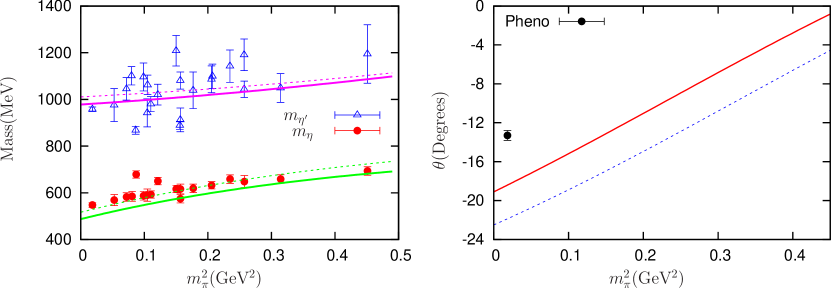
Figure 4: Masses and mixing angle of $\eta$ and $\eta^{\prime}$. The points in the left panel are taken from Ref. Michael:2013vba , which summarizes the data from ETM Michael:2013gka , RBC-UKQCD Christ:2010dd , HSC Dudek:2011tt and UKQCD Gregory:2011sg collaborations. The mixing angle $\theta=(-13.3\pm 0.5)^{\circ}$ extracted in the phenomenological analysis theta-exp for physical masses is plotted in the right panel. The solid lines are obtained by using the physical strange quark mass ($m_{s}=m_{s,{\rm Phys}}$) and the dashed lines come from employing $m_{s}=1.2\,m_{s,{\rm Phys}}$. The value $M_{0}=850$ MeV is taken as input Feldmann:1999uf . We remind the reader this plot is a prediction, not a fit.

In addition, we also take into account the lattice determination of the $\rho(770)$ mass with varying quark masses Lang:2011mn ; Aoki:2011yj ; Pelissier:2012pi ; Dudek:2012xn , which helps us to constrain the vector mass splitting coupling $e_{m}^{V}$ in Eq. (24). For the scalar resonances, as we mentioned previously, we only consider those that survive at large $N_{C}$. In fact, this is not a settled problem yet. For example, the Inverse Amplitude Method analyses RuizdeElvira:2010cs found that the $f_{0}(500)$ or $\sigma$ resonance could fall down to the real axis at large values of $N_{C}$, meaning that it survives as a conventional $\bar{q}q$ state at large $N_{C}$, while the $f_{0}(980)$ disappears in that limit. In the N/D approach, the situation is just the opposite Guo:2011pa ; Guo:2012ym ; Guo:2012yt . However it is interesting to point out that though the resonance trajectories for $N_{C}=3$ to $\infty$ are quite different in the two approaches, there is an important common conclusion: a scalar resonance with mass around 1 GeV at large $N_{C}$ is necessary to fulfill the semi-local duality in $\pi\pi$ scattering. In Refs. Guo:2011pa ; Guo:2012ym ; Guo:2012yt , it was also proved that the 1 GeV scalar resonance at large $N_{C}$ is needed to satisfy the Weinberg sum rules in the scalar and pseudoscalar sectors. Therefore it seems proper to set the bare scalar resonance mass at large $N_{C}$ around 1 GeV. This is also supported by our previous analysis in Ref. Guo:2009hi . In the following we take the result $M_{S}=980$ GeV from Ref. Guo:2009hi as an input while the value of the scalar mass splitting coupling $e_{m}^{S}$ will be fitted in this work, as the value in the previous reference is determined with too large error bars.

The leading order expressions have been employed in our theoretical analysis to relate the squared kaon mass with the varying squared pion mass and $m_{u/d}$:

$$m_{\pi}^{2} = 2B\,m_{u/d}\,,$$ (55)

$$m_{K}^{2} = B\,(m_{s}+m_{u/d})\,=\,\bigg{(}m_{K,{\rm phys}}^{2}-\frac{m_{\pi,{\rm phys}}^{2}}{2}\bigg{)}\alpha_{m_{s}}+\frac{m_{\pi}^{2}}{2}\,,$$ (56)

where $m_{K,{\rm phys}}$ and $m_{\pi,{\rm phys}}$ denote the physical masses of kaon and pion. Different values of $\alpha_{m_{s}}=m_{s}/m_{s,{\rm phys}}$ correspond in this equation to the situations with different strange quark masses whereas $\alpha_{m_{s}}=1$ refers to the physical $m_{s}$ case. We will always take $\alpha_{m_{s}}=1$ in all the fits in this article, considering only lattice simulation data with $m_{s}=m_{s,{\rm phys}}$. Later on, after performing the fit, we will study to what extent our results depend on the linear quark mass relations in Eqs. (55) and (56) by varying $\alpha_{m_{s}}$. Indeed, this insensitivity to higher order corrections was already observed for $m_{\pi}^{2}/(2Bm_{u/d})$ Mpi-lattice ; Durr:2010hr . This ratio was found to show a very small dependence on $m_{u/d}$ in the whole range of values of the simulation Mpi-lattice ; Durr:2010hr , supporting the description given by Eqs. (55) and (56) and used in this article.

Since the $\eta$ and $\eta^{\prime}$ only enter the expressions of $F_{\pi}$ and $F_{K}$ through the chiral loops, it is enough to consider the leading order mixing produced by the Lagrangian (19) for their masses and mixing angle (see App. B for details). The chiral limit of the singlet $\eta_{1}$ mass ($M_{0}$) is by definition independent of the light quark mass and will take the fixed value $M_{0}=850$ MeV in this article Feldmann:1999uf . In Fig. 4 one can see the fair agreement of the LO prediction with lattice simulations Michael:2013vba ; Michael:2013gka ; Christ:2010dd ; Dudek:2011tt ; Gregory:2011sg and previous phenomenological analyses theta-exp for the physical quark mass. The one-parameter fit to lattice data Michael:2013vba ; Michael:2013gka ; Christ:2010dd ; Dudek:2011tt ; Gregory:2011sg for $m_{\eta}$ and $m_{\eta^{\prime}}$ (Fig. 4) yields essentially the same value ($M_{0}\simeq 835$ MeV), very close to the input $M_{0}=850$ MeV which will be employed all through the paper and indistinguishable in Fig. 4 when plotted.

In Fig. 4, the solid lines correspond to our predictions with $\alpha_{m_{s}}=1$ and the dashed lines refer to the case with $\alpha_{m_{s}}=1.2$. It is clear that the change caused by using different strange quark masses in $\eta-\eta^{\prime}$ mixing is mild. On the other hand, it is remarkable that the leading order mixing from $U(3)-\chi$PT can reasonably reproduce the lattice simulation data for the masses of $\eta$ and $\eta^{\prime}$, as shown in the left panel of Fig. 4. In right panel, we show the leading order mixing angle $\theta$ with varying pion masses, i.e. with varying light $u/d$ quark masses. As expected, when the $u/d$ quark mass approaches to the strange quark mass, i.e. the pion mass tends to the kaon mass, there is no mixing between $\eta_{1}$ and $\eta_{8}$, as their mixing strength is proportional to the $SU(3)$ breaking $m_{K}^{2}-m_{\pi}^{2}$. Likewise, this result gives extra support to the linear dependence on the light quark masses for $m_{\phi}^{2}$ assumed in Eqs. (55) and (56) as an approximation in this article.

In the fit, we will use the chiral limit mass of the vector resonance multiplet computed in Ref. Guo:2009hi as an input:

$$\quad M_{V}=764.3~{}{\rm MeV}\,.$$ (57)

Imposing the high energy constraints dictated by QCD is an efficient way to reduce the free couplings in effective field theory. In addition it makes the effective field theory inherit more properties from QCD. In R$\chi$T literature, it is indeed quite popular to constrain the resonance couplings through the high energy behaviors of form factors Rosell-L9-L10 ; Jamin:2001zq , meson-meson scattering Guo:2007ff ; Guo:2011pa , Green functions SanzCillero:2009ap , tau decay form-factors Guo:2008sh ; Guo:2010dv , etc. Among the various constraints obtained in literature, two of them are relevant to our current work

$$c_{d} = {\frac{F_{0}^{2}}{4c_{m}}\,,}$$ (58)

$$G_{V} = {\sqrt{\frac{F_{0}^{2}-2c_{d}^{2}}{3}}\,,}$$ (59)

resulting from the analyses of the scalar form factor Jamin:2001zq and partial-wave $\pi\pi$ scattering Guo:2007ff at large $N_{C}$, respectively.

The renormalization scale $\mu$ will be set at 770 MeV, corresponding the renormalized LECs determined later to their values at that scale.

IV.2 Fit to lattice data

We use the CERN MINUIT package to perform the fit. The values of the six free parameters from the fit read

$$F_{0}=80.0\pm 1.0~{}{\rm MeV}\,,\qquad L_{4}^{\chi PT}=(-0.11\pm 0.06)\times 10^{-3}~{}\,,\qquad L_{5}^{\chi PT}=(0.59\pm 0.08)\times 10^{-3}\,,$$ (60)

$$c_{m}=54.5\pm 3.3~{}{\rm MeV}\,,\qquad e_{m}^{V}=-0.236\pm 0.005\,,\qquad e_{m}^{S}=-0.204\pm 0.024\,,$$

with $\chi^{2}/$d.o.f$=90.8/(52-6)$. The strange quark mass is kept fixed to $m_{s,{\rm phys}}$ in this fit. We point out that one should take the value of $\chi^{2}$ from the fit as a mere orientation of the goodness of the fit rather than in its precise statistical sense: lattice simulation results should not be taken as real experimental data for various quark masses as they are in general highly correlated and systematic uncertainties should be also properly accounted. This gets even worse when combining data from different groups. For a detailed discussion see Ref. Durr:2010hr . The aim of this work is to provide a first quantitative analysis of the potentiality of these type of hadronic observables, i.e. $F_{\pi}$ and $F_{K}$, for the study of resonance properties.

By substituting the results from Eq. (60) in the high energy constraints given in Eqs. (58) and (59) one gets

$$c_{d}=29.3\pm 1.9~{}{\rm MeV}\,,\quad G_{V}=39.5\pm 0.9~{}{\rm MeV}\,.$$ (61)

The negative values for $e_{m}^{R}$ indicate that the resonance masses grow with $m_{q}$ as one can see from Eq. (II.2). They are found in agreement with the previous estimates $e_{m}^{V}=-0.228\pm 0.015$ and $e_{m}^{S}=-0.1\pm 0.9$ Guo:2009hi . The present determinations for $c_{d}$ and $c_{m}$ are compatible with those in Ref. Guo:2009hi : $c_{d}=26\pm 7$ MeV and $c_{m}=80\pm 21$ MeV. Nonetheless, we find large discrepancy for the value of the $\rho-\pi\pi$ coupling given in Ref. Guo:2009hi : $G_{V}=63.9\pm 0.6$ MeV. The reason for the large discrepancies of the $G_{V}$ values will be analyzed in detail in next section.

In the left panel of Fig. 5, we show our fit results together with the lattice data for $M_{\rho}$ with different pion masses, which are originally taken from Refs. Lang:2011mn ; Aoki:2011yj ; Pelissier:2012pi ; Dudek:2012xn . Due to the large error bars of these data, the stringent constraint on the vector mass splitting parameter $e_{m}^{V}$ comes from the determination of physical masses of $\rho$, $K^{*}$ and $\phi$, which are shown in the right panel of Fig. 5. This explains in part the very similar results between our current value for $e_{m}^{V}$ and that in Ref. Guo:2009hi .

The light-blue and crisscross shaded areas surrounding the solid lines in Figs. 5 and 6 represent our estimates of the 68% confidence level (CL) error bands. In order to obtain these uncertainty regions we first generate large sets of parameter configurations by varying all our 6 fit parameters around their central values randomly via a Monte Carlo (MC) generator; then we use these large amount of parameter configurations to calculate the $\chi^{2}$ and keep only the configurations with $\chi^{2}$ smaller than $\chi_{0}^{2}+\Delta\chi^{2}$, being $\chi_{0}^{2}$ the minimum chi-square obtained from the fit. The 68% CL region is given by $\Delta\chi^{2}=7.04$ for a 6–parameter fit . The successful parameter configurations provide the 68% CL error bands. In such a way, the correlations between the different fit parameters in Eq. (60) have been taken into account when plotting the error bands in Figs. 5 and 6.

Both our fit results and the lattice simulation data for $F_{\pi}$ and $F_{K}$ with varying pion masses are shown in the left panel of Fig. 6. The lattice data for $F_{\pi}$ and $F_{K}$ are taken from MILC Davies:2003fw ; Davies:2003ik , RBC and UKQCD Aoki:2010dy ; Arthur:2012opa . Concerning the data from Refs. Aoki:2010dy ; Arthur:2012opa , we only consider those that are simulated with the physical strange quark mass and the unitary points. In the right panel, we give the plots for the ratio $F_{K}/F_{\pi}$ Durr:2010hr . Even though the fit is performed with $m_{s}=m_{s,{\rm phys}}$, we have also plotted in Fig. 6 the predictions for $F_{\pi}$ and $F_{K}$ with $m_{s}=1.2\,m_{s,{\rm phys}}$ . For this we have used the fit values from Eq. (60). In the left panel of Fig. (6), one can see how the results with physical strange quark mass (solid lines) vary when one instead uses $\alpha_{m_{s}}=1.2$ in Eq. (56) (dashed lines). In the right panel of Fig. 6, the solid red line (lower) corresponds to the fit result with the perturbative expansion of $F_{K}/F_{\pi}$ up to one loop order in Eq. (54) with $m_{s}=m_{s,{\rm phys}}$, whereas the dash-dotted red (upper) line uses Eq. (54) with $m_{s}=1.2\,m_{s,{\rm phys}}$. The blue double-dashed (lower) line represents the unexpanded value of $F_{K}/F_{\pi}$ extracted directly from $F_{\pi}$ and $F_{K}$ from Eq. (51) with $m_{s}=m_{s,{\rm phys}}$, while the blue dashed (upper) line uses the same unexpanded expression but with $m_{s}=1.2\,m_{s,{\rm phys}}$.

Using a value of the strange quark mass 20% larger than the physical one only induces slight changes for $F_{\pi}$ and $F_{K}$ in the region of $m_{\pi}\leq 500$ MeV, indicating the smaller sensitivity of these two quantities to the linear quark mass dependence for $m_{\phi}^{2}$ assumed in Eqs. (55) and (56). Notice that $F_{\pi}$ decreases when $m_{s}$ increases, while $F_{K}$ grows. The reason is the different way how $m_{s}$ enters in these two observables: through loops and $1/N_{C}$ suppressed in $F_{\pi}$; in the valence quarks and contributing at LO in $1/N_{C}$ for $F_{K}$. This explains the larger shift observed in the $F_{K}/F_{\pi}$ ratio when varying the strange quark mass (see the right panel in Fig. 6).

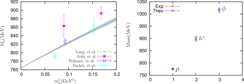
Figure 5: Fit results for the vector masses. The left panel shows the square pion mass dependence of $M_{\rho}$. The lattice data in this panel are taken from Refs. Lang:2011mn ; Aoki:2011yj ; Pelissier:2012pi ; Dudek:2012xn . The right panel shows the masses of $\rho(770)$, $K^{*}(892)$ and $\phi(1020)$ with the physical pion mass. The shaded area in the left panel and the empty circles in the right panel represent our estimation of the error bands, which are explained in detail in the text.

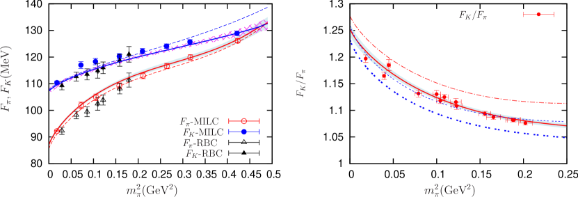
Figure 6: Fit results for $F_{\pi}$, $F_{K}$, together with the lattice data from MILC Davies:2003fw ; Davies:2003ik , RBC and UKQCD Aoki:2010dy ; Arthur:2012opa collaborations are shown in the left panel. The light blue and crisscross band provide the 68% CL regions in both plots. In the right panel, we plot the ratio $F_{K}/F_{\pi}$ together with the lattice data from Ref. Durr:2010hr . The leftmost data points in each panel correspond to the physical mass values, which are taken from PDG Beringer:1900zz . The solid lines in the left panel are the fit results with physical strange quark mass. The solid red (lower) and double-dashed blue (lower) lines in the right-hand plot refer to the expanded (Eq. (54)) and unexpanded (Eq. (51)) expressions for $F_{K}/F_{\pi}$ with $\alpha_{m_{s}}=1$, respectively. The dashed lines in the left panel correspond to $\alpha_{m_{s}}=1.2$. The same applies to the dash-dotted red (upper) and dashed blue (upper) lines in the right-hand plot, which refer to the expanded (Eq. (54)) and unexpanded (Eq. (51)) expressions for $F_{K}/F_{\pi}$, respectively.

IV.3 Anatomy of the fit parameters: correlations

For the scalar resonance parameters $c_{d}$ and $c_{m}$, our current results are quite compatible with those determined in many other processes rcht89 ; Guo:2009hi ; Guo:2011pa ; Guo:2012yt ; theta-Nc ; Jamin:2001zq . However, the present determination of $G_{V}$ in Eq. (61), is clearly lower than the usual results from phenomenological analyses, which prefer values around 60 MeV rcht89 ; Guo:2009hi ; Guo:2011pa ; Guo:2012yt . One way out of this problem is to free $G_{V}$ in our fit, instead of imposing its large–$N_{C}$ high energy constraint from Eq. (59).

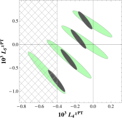
Figure 7: 68% CL regions for $L_{4}^{\chi PT}(\mu)$ and $L_{5}^{\chi PT}(\mu)$ at $\mu=770$ MeV for the fits with $G_{V}$ fixed to $40,\,50,\,60$ and $70$ MeV (respectively from top-right to bottom-left). Here and in the following plots the crisscross area (left-hand side of this figure) represents the region forbidden by the paramagnetic inequality $F^{n_{f}=3}\,<\,F^{n_{f}=2}$, which implies $L_{4}^{\chi PT}(\mu)>-0.4\cdot 10^{-3}$ for $\mu=770$ MeV Ecker:2013pba ; DescotesGenon:1999uh . The light-green ellipses come from fits to data points with $m_{\pi}<500$ MeV and the darker gray ones from the fits to all data.

A first test is provided by setting $G_{V}$ to particular values. In Fig. 7, we plot the 68% CL regions for $L_{4}^{\chi PT}$ and $L_{5}^{\chi PT}$ for the fits with $G_{V}$ fixed to $G_{V}=40,50,60,70$ MeV (ellipses from top-right to bottom-left in Fig. 7, respectively; Gaussianity is assumed). This shows how the $\rho-\pi\pi$ coupling affects the determinations of $L_{4}^{\chi PT}$ and $L_{5}^{\chi PT}$: smaller values of $G_{V}$ lead to a closer agreement with the standard $\chi$PT phenomenology Bijnens:2011tb ; gl845 . On the other hand, larger values of $G_{V}$ tend to decrease the values of both LECs; eventually, for a large enough $\rho-\pi\pi$ coupling, $L_{5}^{\chi PT}$ turns negative and $L_{4}^{\chi PT}$ violates the paramagnetic inequality $F^{n_{f}=3}\,<\,F^{n_{f}=2}$ ($L_{4}^{\chi PT}(\mu)>-0.4\cdot 10^{-3}$ for $\mu=770$ MeV Ecker:2013pba ; DescotesGenon:1999uh ). This effect cannot be attributed to an inappropriate description of the kaon and pion masses in Eqs. (55) and (56) nor the fact of neglecting operators of the Lagrangian whose contributions to $F_{\phi}$ are suppressed by both $1/N_{C}$ and $m_{\phi}^{4}/M_{S}^{4}$. This can be neatly observed in Fig. 7, where the black ellipses are given by the fit to the full set of lattice data whereas only the data with $m_{\pi}<500$ MeV are used in the fits that provide the light-green regions. Reducing the number of data points in the large pion mass region obviously leads to a consistent enlargement of the uncertainty regions but does not modify at all the strong correlation with $G_{V}$.

A second test consists on exploring two alternative versions of the high energy constraints for the $\rho-\pi\pi$ coupling in Eq. (59): $G_{V}=F_{0}/\sqrt{2}$ ksrf and $G_{V}=F_{0}/\sqrt{3}$ Guo:2007ff ; Guo:2011pa . The former constraint corresponds to the original Kawarabayashi-Suzuki-Riazuddin-Fayyazuddin (KSRF) relation while the latter is the extended KSRF relation obtained by including the crossed-channel contributions and ignoring the scalar resonances in $\pi\pi$ scattering. We obtain $G_{V}\sim 58$ MeV for $G_{V}=F_{0}/\sqrt{2}$ and $G_{V}\sim 47$ MeV for $G_{V}=F_{0}/\sqrt{3}$, with the chiral coupling $F_{0}$ remaining always stable and with a value around 82 MeV. In both situations, we confirm the findings we obtained previously when $G_{V}$ was fixed at the specific values $40$, $50$, $60$ and $70$ MeV (see Fig. 7): we observe strong anti-correlations between $L_{4}^{\chi PT}$ and $L_{5}^{\chi PT}$ and their values are strongly affected by $G_{V}$ in the way discussed before. The values of $L_{4}^{\chi PT}$ and $L_{5}^{\chi PT}$ follow closely the trend shown in Fig. 7: the smaller $G_{V}$ becomes, the more negative $L_{4}^{\chi PT}$ and $L_{5}^{\chi PT}$ turn. Hence we conclude that our second test based on using different high energy constraints for $G_{V}$ confirms our former findings and do not reveal new information with respect to the first test, where $G_{V}$ was fixed at specific values.

We will proceed now with our third test: $G_{V}$ will be set free and fitted together with the other six parameter from the previous analysis. Statistically speaking, we do not find any significant improvement of the fit quality by releasing this additional free parameter, but we do see obvious changes with respect to the values in Eq. (60), which now turn out to be

$$F_{0}=83.5\pm 1.5~{}{\rm MeV}\,,\qquad L_{4}^{\chi PT}=(-0.31\pm 0.10)\times 10^{-3}~{}\,,\qquad L_{5}^{\chi PT}=(-0.46\pm 0.33)\times 10^{-3}\,,$$

$$c_{m}=64.1\pm 3.7~{}{\rm MeV}\,,\qquad e_{m}^{V}=-0.236\pm 0.004\,,\qquad e_{m}^{S}=-0.540\pm 0.088\,,$$

$$G_{V}=63.0\pm 6.4~{}{\rm MeV}\,,$$ (62)

with $\chi^{2}/$(d.o.f)$=80.0/(52-7)$. The fit quality resulting in this case is quite similar to that in the previous section. By substituting the results from Eq. (IV.3) in the scalar form-factor high energy constraints from Eq. (58) one obtains

$$c_{d} = \,(\,27.2\,\pm\,1.8\,)\,{\rm MeV}\,.$$ (63)

The most striking change happens for $L_{5}^{\chi PT}$, whose sign becomes negative. However, according to most phenomenological determinations of $L_{5}^{\chi PT}$ in literature Bijnens:2011tb ; Ecker:2010nc ; Ecker:2013pba its value must be positive. Also R$\chi$T predicts a positive $L_{5}^{\chi PT}$ at large $N_{C}$ rcht89 . Hence the resulting parameters in Eq. (IV.3) do not seem to correspond to the physical solution. The reason behind this is the strong correlations between different parameters: we observe that the parameter $G_{V}$ is strongly correlated with all of the other parameters. The only exception is $e_{m}^{V}$, which is mostly uncorrelated and is essentially determined by the $\rho(770)-K^{*}(892)-\phi(1020)$ splitting. The correlations are summarized in Figs. 8 and 9 (Gaussianity is assumed). In Fig. 8 we provide the correlation between $G_{V}$ and the other fit variables. One can clearly see that the parameter $G_{V}$, which rules the $\rho-\pi\pi$ interaction vertex in the chiral limit, is highly correlated with almost all the other parameters. By observing this plots, one can easily understand why we have obtained such different values for $L_{5}^{\chi PT}$ in Eqs. (60) (with $G_{V}$ constrained through Eq. (59)) and (IV.3) (free $G_{V}$): the values for $G_{V}$ are very different in the two fits and a positive (negative) $L_{5}^{\chi PT}$ requires a small (large) value for $G_{V}$ (see bottom-center panel in Fig. 8).

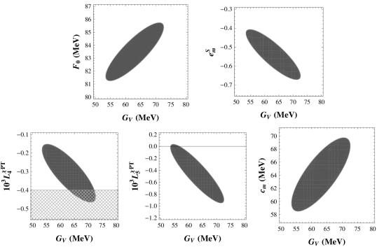
Figure 8: $68\%$ CL regions for $G_{V}$ and other parameter. All these plots correspond to the 7-parameter analysis in Eq. (IV.3), where $G_{V}$ is also fitted.

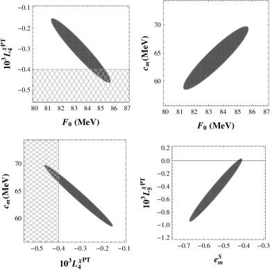
Figure 9: $68\%$ CL regions for sets of two couplings. All these plots correspond to the 7-parameter analysis in Eq. (IV.3), where $G_{V}$ is also fitted.

In the top left panel in Fig. 9, one can clearly observe an evident anti-correlation between $F_{0}$ and $L_{4}^{\chi PT}$, noticed in previous works Ecker:2010nc ; Ecker:2013pba . In addition, we observe a strong anti-correlation for $L_{4}^{\chi PT}-c_{m}$ and an obvious correlation for $L_{5}^{\chi PT}-e_{m}^{S}$, as shown in the two panels in the bottom row of Fig. 9. In Ref. DescotesGenon:1999uh , a lower bound on the value of $L_{4}^{\chi PT}$ has been proposed by requiring that the pNGB decay constant in $SU(3)$ chiral limit must be smaller than the decay constant in the $SU(2)$ limit. This gives the inequality $L_{4}^{\chi PT}>-0.4\times 10^{-3}$ for $\mu=770$ MeV Ecker:2013pba . It is interesting to point out that this lower bound from $L_{4}^{\chi PT}$ leads to lower or upper bounds for some of the parameters considered in our work because of the strong correlations. This can be roughly read from Figs. 8 and 9: $G_{V}<72$ MeV, $F_{0}<86$ MeV and $c_{m}<68$ MeV. On the other hand, one can observe in Figs. 8 and 9 that in order to have a positive $L_{5}^{\chi PT}$ one has the rough bounds $G_{V}<60$ MeV and $e_{m}^{S}>-0.45$. Combining the paramagnetic inequality for $L_{4}^{\chi PT}$ DescotesGenon:1999uh ; Ecker:2013pba and the phenomenological bound $L_{5}^{\chi PT}>0$ leads to the rough estimates $F_{0}<86$ MeV, $G_{V}<60$ MeV, $c_{m}<68$ MeV and $e_{m}^{S}>-0.45$.

In order to further test the relations between $G_{V}$ and other parameters, we want to see the impact of including a second scalar nonet. The contributions from the second scalar nonet to the decay constants in Appendix C and the matching conditions in Eqs. (48)-(50) share the same expressions as the lowest scalar multiplet, but with obvious replacements of the couplings $c_{d}$, $c_{m}$, $e_{m}^{S}$ by $c_{d}^{\prime}$, $c_{m}^{\prime}$ and $e_{m}^{S^{\prime}}$. The chiral limit resonance mass $M_{S^{\prime}}$ of the excited nonet $S^{\prime}$ should be replaced as well. The introduction of the second scalar nonet will also affect the high energy constraints in Eqs. (58) and (59), which now become Jamin:2001zq ; Guo:2007ff

$$c_{d} = {\frac{F_{0}^{2}-4c_{d}^{\prime}c_{m}^{\prime}}{4c_{m}}\,,}$$ (64)

$$G_{V} = {\sqrt{\frac{F_{0}^{2}-2c_{d}^{2}-2{c_{d}^{\prime}}^{2}}{3}}\,.}$$ (65)

Phenomenologically, the $S^{\prime}$ parameters are poorly known in the literature and we do not expect to obtain precise values from our analysis. In order to perform our quantitative estimate of the role of the second scalar nonet, we take the part of the outcomes from Ref. Jamin:2000wn as inputs. More precisely, we take $c_{m}^{\prime}=c_{d}^{\prime}$ and $M_{S^{\prime}}=2.57$ GeV (preferred fit values from Ref. Jamin:2000wn , Eq.(6.10) therein).  The mass splitting parameter $e_{m}^{S^{\prime}}$ is even worse known than $c_{d}^{\prime}$ and $c_{m}^{\prime}$. In our rough analysis we will set its value to zero. Thus, we only have one free parameter $c_{d}^{\prime}$ from the second scalar nonet. In Refs. Jamin:2000wn ; Jamin:2001zq , $c_{d}^{\prime}$ was obtained through the constraint $F_{0}^{2}=4(c_{d}c_{m}+c_{d}^{\prime}c_{m}^{\prime})$ by using $F_{0}=F_{\pi}=92.4$ MeV, whereas in our work $F_{0}$ is truly the pion decay constant in the chiral limit. Hence, instead of taking the result of $c_{d}^{\prime}$ from Ref. Jamin:2000wn , we fit its value together with the chiral coupling $F_{0}$.

The fit result with the new constraints in Eqs. (64) and (65) (two scalar multiplets) turn out to be quite similar to the outcomes in Eq. (60) with only one scalar nonet in the high-energy constraints (58) and (59). The additional coupling becomes $c_{d}^{\prime}\simeq(11\pm 30)$ MeV, a value compatible with the preferred determination in Ref. Jamin:2000wn and alternative fits therein. In this work we reconfirm the large uncertainty for $c_{d}^{\prime}$ obtained from $K\pi$ scattering Jamin:2000wn . We have also tried other fits where high-energy relation (65) is released and $G_{V}$ is freed and fitted. The $\rho-\pi\pi$ coupling has been also set in later fits to the particular values $G_{V}=F_{0}/\sqrt{2}$ ksrf and $G_{V}=F_{0}/\sqrt{3}$ Guo:2007ff ; Guo:2011pa . In all these cases the results tend to produce small central values for $c_{d}^{\prime}$ but with large uncertainties. As a result, the inclusion of the second scalar nonet barely changes our conclusions derived previously with only one scalar nonet.

In summary: the present determination for $F_{0}$, the $n_{f}=3$ pNGB decay constant in the chiral limit, is rather stable, ranging from 78 to 86 MeV for any value of $G_{V}$ in the range $40\sim 70$ MeV. Our current determinations of the $\chi$PT LECs $L_{4}^{\chi PT}$ and $L_{5}^{\chi PT}$ can not be pinned down to a precise range due to their strong correlations with the resonance couplings, which are typically determined through some phenomenological processes with non-negligible uncertainties. Among the various resonance couplings, $G_{V}$ turns out to be the crucial one to prevent us from making precise determinations. In the case of imposing the high energy constraint on $G_{V}$ from Eq. (59), obtained from the discussion of the partial wave $\pi\pi$ scattering at LO in $1/N_{C}$ Guo:2007ff , the corresponding fit results in Eq. (60) are more or less compatible with the state-of-art determinations of the $\chi$PT LECs. We regard these results as our preferred ones in this work. Nonetheless, one should always bear in mind the strong correlations shown in Figs. 8 and 9.

V Conclusions

The aim of this work is to provide a first quantitative test of the potentiality of these type of hadronic observables, such as the pNGB decay constants, for the study of resonance properties. We have calculated the pion and kaon weak decay constants within the framework of R$\chi$T up to NLO in $1/N_{C}$, this is, up to the one-loop level. In addition to the octet of light pNGB, we have explicitly included the singlet $\eta_{1}$ and the lightest vector and scalar resonance multiplets surviving at large $N_{C}$. However, we want to remark that the errors provided here should be considered with quite some care, as we have combined data from various simulation groups, ignoring correlations and systematic and lattice spacing uncertainties.

Our one-loop expressions for $F_{\pi}$ and $F_{K}$ in R$\chi$T have been properly matched to $SU(3)$ $\chi$PT up to ${\cal O}{(p^{4})}$ in the small quark mass regime, providing prediction for the chiral LECs in terms of the R$\chi$T parameters. As higher order corrections from $\chi$PT are partly incorporated through the resonance loops, the present calculation provides an alternative approach which complements previous $\chi$PT analyses Ecker:2013pba ; FP-Op6 ; lattice-TBC ; Bernard:2011 . The price to pay in the latter is, however, the vast amount of $\chi$PT couplings one needs to consider in the full ${\cal O}(p^{6})$ expression. In our work, the resonances are assumed to play a crucial role instead, ruling the dynamics of the decay constant.

We have extended the work from Ref. Soto:2011ap (which incorporated the scalar effects at one loop) by considering also the impact of vector resonances in the loops. One of the fundamental conclusions in our study is that the vectors play a crucial role in the one-loop decay constant, being crucial parameters such as $F_{0}$, $L_{4}^{\chi PT}$ and $L_{5}^{\chi PT}$ very correlated with the value of the $\rho-\pi\pi$ coupling $G_{V}$. Low values of $G_{V}$, around 40 MeV, lead to larger values of $L_{4}^{\chi PT}$ and $L_{5}^{\chi PT}$, in closer agreement with standard $\chi$PT determinations Bijnens:2011tb . Due to the $L_{4}^{\chi PT}\leftrightarrow F_{0}$ anti-correlation this yields a small value for $F_{0}$, around 80 MeV. On the other hand, a $G_{V}$ coupling in the range $60\sim 70$ MeV seems to be in better agreement with vector resonance phenomenology rcht89 ; SD-RChT ; Guo:2007ff ; Guo:2009hi but generates a far too negative value for both $L_{4}^{\chi PT}$ and $L_{5}^{\chi PT}$, in clear contradiction with $\chi$PT determinations Bijnens:2011tb and QCD paramagnetic inequalities  DescotesGenon:1999uh ($L_{4}^{\chi PT}>-0.4\cdot 10^{-3}$ for $\mu=770$ MeV Ecker:2013pba ). Nonetheless, in spite of this big effect on the ${\cal O}(p^{4})$ LECs, $F_{0}$ happens to be very stable and only rises up to roughly 85 MeV. Clearly, this interplay between vector resonance loops and $\chi$PT loops deserves further investigation in future works.

In the fit where $G_{V}$ is fixed to 40, 50, 60 and 70 MeV we observe clearly how the coupling $F_{0}$ evolves from $80$ up to $85$ MeV. Although the upper value is compatible with recent ${\cal O}(p^{6})$ estimates Ecker:2013pba , other analyses favor values of $F_{0}$ below 80 MeV Bernard:2011 . In general, there is no agreement yet (see FLAG’s review FLAG:2013 and references therein) and the strong anti-correlation between $F_{0}$ and $L_{4}^{\chi PT}$ found here and in previous works Bijnens:2011tb ; Ecker:2013pba transfers this uncertainty to the ${\cal O}(p^{4})$ LEC $L_{4}^{\chi PT}$.

The analysis of $F_{\pi}$, $F_{K}$ Davies:2003fw ; Davies:2003ik ; Aoki:2010dy ; Arthur:2012opa and $F_{K}/F_{\pi}$ Durr:2010hr was carried out in combination with a study of the quark mass dependence of the $\rho(770)$, $\eta$ and $\eta^{\prime}$ masses. The simple quark mass dependence of the vector multiplet mass introduced through $e_{m}^{V}$ perfectly accommodates the $M_{\rho}$ lattice data Lang:2011mn ; Aoki:2011yj ; Pelissier:2012pi ; Dudek:2012xn and the observed splitting of the physical vector multiplet Beringer:1900zz (Fig. 5). Likewise, the LO prediction for the $\eta-\eta^{\prime}$ mixing is found to be in reasonable agreement with lattice data Michael:2013vba ; Michael:2013gka ; Christ:2010dd ; Dudek:2011tt ; Gregory:2011sg (Fig. 4). We find that our theoretical formulas can reproduce the lattice data from the physical pion mass up to roughly $m_{\pi}=700$ MeV. This result gives support to the linear relation between the pNGB and quark masses from Eqs. (55) and (56), assumed all along the article.

Based on the promising fact that the present framework performs a reasonable chiral extrapolation for $F_{\pi}$ and $F_{K}$ within a broad range of pion masses, a similar study on the masses of $\pi$, $K$, or even $\eta$ and $\eta^{\prime}$ should be pursued within R$\chi$T up to NLO in $1/N_{C}$. This would also allow us to go beyond the linear quark mass dependence considered for the squared masses of the pion and kaon in this article. We think this might help to set further and more stringent constraints on the low energy constants of the $\chi$PT Lagrangian.

Appendix A Feynman integrals

The explicit expressions for the loop functions used in this work are given by

$$A_{0}(m^{2}) = \displaystyle{\int}\frac{\displaystyle d^{d}k}{\displaystyle(2\pi)^{d}}\,\frac{\displaystyle 1}{\displaystyle k^{2}-m^{2}}\quad=\quad\frac{i}{16\pi^{2}}m^{2}\bigg{(}\frac{1}{\hat{\epsilon}}-\ln{\frac{m^{2}}{\mu^{2}}}\bigg{)}\,,$$

$$B_{0}(q^{2},M^{2},m^{2}) = \displaystyle{\int}\frac{\displaystyle d^{d}k}{\displaystyle(2\pi)^{d}}\,\frac{\displaystyle 1}{\displaystyle(k^{2}-m^{2})\,((q-k)^{2}-M^{2})}$$

$$\quad=\quad\frac{i}{16\pi^{2}}\bigg{[}\frac{1}{\hat{\epsilon}}+1-\frac{1}{2}\ln{\frac{M^{2}m^{2}}{\mu^{4}}}+\frac{\Delta}{2s}\ln{\frac{m^{2}}{M^{2}}}-\frac{\nu}{2s}\ln\frac{(\Sigma-s-\nu)^{2}}{4M^{2}m^{2}}\bigg{]}\,,$$

$$B_{0}^{\prime}(s,M^{2},m^{2}) = \frac{dB_{0}(s,M,m)}{ds}=\frac{i}{16\pi^{2}}\bigg{[}-\frac{\Delta}{2s^{2}}\ln{\frac{m^{2}}{M^{2}}}-\frac{1}{s}+\frac{\Delta^{2}-\Sigma s}{2\nu s^{2}}\ln\frac{(\Sigma-s-\nu)^{2}}{4M^{2}m^{2}}\bigg{]}\,,$$

where

$$\frac{1}{\hat{\epsilon}} = \mu^{-2\epsilon}\,\left(\frac{1}{\epsilon}-\gamma_{E}+\ln{4\pi}+1\right)\quad=\quad\frac{\displaystyle 1}{\displaystyle\epsilon}-\gamma_{E}+\ln{4\pi}+1-\ln\mu^{2}+{\cal O}(\epsilon)\,,\qquad(\epsilon=2-\frac{D}{2})\,,$$

$$\Delta = M^{2}-m^{2}\,,\qquad\Sigma=M^{2}+m^{2}\,,\qquad\nu=\sqrt{\big{[}s-(M+m)^{2}\big{]}\big{[}s-(M-m)^{2}\big{]}}\,.$$ (67)

Appendix B $\eta_{1}-\eta_{8}$ mixing

After the diagonalization of $\eta_{1}-\eta_{8}$ at leading order, we have the physical $\eta$ and $\eta^{\prime}$ states at this order and their masses and the mixing angle can be found in many references in literature, such as Ref. Guo:2011pa . We give the explicit formulas for the sake of completeness

$$m_{\eta}^{2} = \frac{M_{0}^{2}}{2}+m_{K}^{2}-\frac{\sqrt{M_{0}^{4}-\frac{4M_{0}^{2}\Delta^{2}}{3}+4\Delta^{4}}}{2}\,,$$ (68)

$$m_{\eta^{\prime}}^{2} = \frac{M_{0}^{2}}{2}+m_{K}^{2}+\frac{\sqrt{M_{0}^{4}-\frac{4M_{0}^{2}\Delta^{2}}{3}+4\Delta^{4}}}{2}\,,$$ (69)

$$\sin{\theta} = -\left(\sqrt{1+\frac{\big{(}3M_{0}^{2}-2\Delta^{2}+\sqrt{9M_{0}^{4}-12M_{0}^{2}\Delta^{2}+36\Delta^{4}}\big{)}^{2}}{32\Delta^{4}}}~{}\right)^{-1}\,,$$ (70)

with $\Delta^{2}=m_{K}^{2}-m_{\pi}^{2}$. Notice that $m_{\eta}$, $m_{\eta^{\prime}}$ and $\theta$ are fully determined at this order by $m_{\pi}$, $m_{K}$ and $M_{0}$.

In the ideal mixing case ($M_{0}=0$) one gets $m_{\eta}^{2}=m_{\pi}^{2}$, $m_{\eta^{\prime}}^{2}=2m_{K}^{2}-m_{\pi}^{2}$ and ${\sin\theta=-\sqrt{2/3}}$. On the other hand, in the chiral limit $m_{\pi},\,m_{K}\to 0$ the physical masses and mixing become $m_{\eta}^{2}=0$, $m_{\eta^{\prime}}^{2}=M_{0}^{2}$ and $\theta=0$.

Appendix C Feynman diagrams up to NLO in $1/N_{C}$

C.1 The pion self-energy

As shown in Fig. 2, there are three types of Feynman diagrams contributing to the pNGB self-energy $\Sigma^{\pi}$. For the diagram (a) in this figure, the explicit calculation from Lagrangian in Eq. (26) leads to

$$\Sigma^{\pi-a}= \bigg{(}1-\frac{\displaystyle\widetilde{F}^{2}}{\displaystyle F_{0}^{2}}\bigg{)}p^{2}-\bigg{(}1-\frac{\displaystyle\hat{F}^{2}}{\displaystyle F_{0}^{2}}\bigg{)}m_{\pi}^{2}\,\,\,+\,\,\,\frac{4\widetilde{L}_{12}}{F_{0}^{2}}(p^{2}-m_{\pi}^{2})^{2}-\frac{8\widetilde{L}_{11}}{F_{0}^{2}}m_{\pi}^{2}(p^{2}-m_{\pi}^{2})$$

$$-\frac{8\widetilde{L}_{4}}{F_{0}^{2}}(2m_{K}^{2}+m_{\pi}^{2})p^{2}-\frac{8}{F_{0}^{2}}(\widetilde{L}_{5}+\frac{c_{d}c_{m}}{M_{S}^{2}})m_{\pi}^{2}\,p^{2}+\frac{16\widetilde{L}_{6}}{F_{0}^{2}}(2m_{K}^{2}+m_{\pi}^{2})m_{\pi}^{2}+\frac{16}{F_{0}^{2}}(\widetilde{L}_{8}+\frac{c_{m}^{2}}{2M_{S}^{2}})m_{\pi}^{4}\,.$$

where we have used the linear relations (55) and (56) to rewrite the quark masses in terms of the pion and kaon masses. The tree-level contribution from the operators in the second line of Eq. (30) have been also taken into account.

About the diagram (b) in Fig. 2, its contribution to the pion self-energy is the same as in $U(3)$ $\chi$PT, which is calculated by using leading order Lagrangian in Eq. (19) and reads

$$\Sigma^{\pi-b} =\frac{i}{3F_{0}^{2}}(2p^{2}-\frac{m_{\pi}^{2}}{2})A_{0}(m_{\pi}^{2})+\frac{i}{3F_{0}^{2}}(p^{2}-m_{\pi}^{2})A_{0}(m_{K}^{2})+\frac{-i}{2F_{0}^{2}}\frac{(c_{\theta}-\sqrt{2}s_{\theta})^{2}}{3}m_{\pi}^{2}A_{0}(m_{\eta}^{2})$$ (72)

$$+\frac{-i}{2F_{0}^{2}}\frac{(\sqrt{2}c_{\theta}+s_{\theta})^{2}}{3}m_{\pi}^{2}A_{0}(m_{\eta^{\prime}}^{2})\,.$$

The diagram (c) in Fig. 2 receives contributions both from scalar and vector resonances. Let us take the self-energy for the $\pi^{-}$ for illustration. There are five possible combinations of scalar resonance and pseudoscalar meson running inside the loop: $\sigma\pi^{-}$, $\kappa^{-}K^{0}$, $\kappa^{0}K^{-}$, $a_{0}^{-}\eta$ and $a_{0}^{-}\eta^{\prime}$, which will be labeled as $-i\Sigma^{\pi-cSj}$, with $j=1,2,3,4,5$, respectively. About the vector, there are four possible combinations: $\rho^{-}\pi^{0}$, $\rho^{0}\pi^{-}$, $K^{*0}K^{-}$ and $K^{*-}K^{0}$ , which will be labeled as $-i\Sigma^{\pi-cVj}$, with $j=1,2,3,4$, respectively.

The explicit results of $\Sigma^{\pi-cSj}$ for $j=1,2,3,4,5$ are

$$\Sigma^{\pi-cS1} =\frac{i2c_{d}^{2}}{F_{0}^{4}}\bigg{[}\,(3p^{2}+m_{\pi}^{2}-M_{\sigma}^{2})A_{0}(M_{\sigma}^{2})-(m_{\pi}^{2}+p^{2}-M_{\sigma}^{2})A_{0}(m_{\pi}^{2})$$ (73)

$$\qquad\qquad+(m_{\pi}^{2}+p^{2}-M_{\sigma}^{2})^{2}B_{0}(p^{2},M_{\sigma}^{2},m_{\pi}^{2})\,\bigg{]}$$

$$\quad-\frac{i8c_{d}c_{m}}{F_{0}^{4}M_{S}^{2}}m_{\pi}^{2}M_{\sigma}^{2}\bigg{[}\,(m_{\pi}^{2}+p^{2}-M_{\sigma}^{2})B_{0}(p^{2},M_{\sigma}^{2},m_{\pi}^{2})+A_{0}(M_{\sigma}^{2})-A_{0}(m_{\pi}^{2})\,\bigg{]}$$

$$\quad+\frac{i8c_{m}^{2}}{F_{0}^{4}M_{S}^{4}}m_{\pi}^{4}\bigg{[}\,M_{\sigma}^{4}B_{0}(p^{2},M_{\sigma}^{2},m_{\pi}^{2})+(m_{\pi}^{2}+p^{2}+M_{\sigma}^{2})A_{0}(m_{\pi}^{2})\,\bigg{]}\,,$$

$$\Sigma^{\pi-cS2}=\Sigma^{\pi-cS3} =\frac{ic_{d}^{2}}{F_{0}^{4}}\bigg{[}\,(3p^{2}+m_{K}^{2}-M_{\kappa}^{2})A_{0}(M_{\kappa}^{2})-(m_{K}^{2}+p^{2}-M_{\kappa}^{2})A_{0}(m_{K}^{2})$$ (74)

$$\qquad\qquad+(m_{K}^{2}+p^{2}-M_{\kappa}^{2})^{2}B_{0}(p^{2},M_{\kappa}^{2},m_{K}^{2})\,\bigg{]}$$

$$\quad-\frac{i2c_{d}c_{m}}{F_{0}^{4}M_{S}^{2}}\bigg{\{}\,\big{[}2m_{\pi}^{2}M_{\kappa}^{2}+(m_{K}^{2}-m_{\pi}^{2})(M_{\kappa}^{2}-s-m_{K}^{2})\big{]}A_{0}(M_{\kappa}^{2})$$

$$\qquad\qquad+\big{[}-2m_{\pi}^{2}M_{\kappa}^{2}+(m_{K}^{2}-m_{\pi}^{2})(m_{K}^{2}-s-M_{\kappa}^{2})\big{]}A_{0}(m_{K}^{2})$$

$$\qquad\qquad+\big{[}2m_{\pi}^{2}M_{\kappa}^{2}(s+m_{K}^{2}-M_{\kappa}^{2})$$

$$\qquad\qquad\qquad+(m_{K}^{2}-m_{\pi}^{2})(s^{2}-M_{\kappa}^{4}-m_{K}^{4}+2m_{K}^{2}M_{\kappa}^{2})\big{]}B_{0}(p^{2},M_{\kappa}^{2},m_{K}^{2})\,\bigg{\}}$$

$$\quad+\frac{ic_{m}^{2}}{F_{0}^{4}M_{S}^{4}}\bigg{\{}\,\big{[}-4m_{\pi}^{2}(m_{K}^{2}-m_{\pi}^{2})M_{\kappa}^{2}+(m_{K}^{2}-m_{\pi}^{2})^{2}(m_{K}^{2}-s-M_{\kappa}^{2})\big{]}A_{0}(M_{\kappa}^{2})$$

$$+\big{[}4m_{\pi}^{4}(s+m_{K}^{2}+M_{\kappa}^{2})+4m_{\pi}^{2}(m_{K}^{2}-m_{\pi}^{2})(2s+M_{\kappa}^{2})$$

$$\quad+(m_{K}^{2}-m_{\pi}^{2})^{2}(3s+M_{\kappa}^{2}-m_{K}^{2})\big{]}A_{0}(m_{K}^{2})$$

$$+\big{[}4m_{\pi}^{4}M_{\kappa}^{4}+4m_{\pi}^{2}(m_{K}^{2}-m_{\pi}^{2})(s+M_{\kappa}^{2}-m_{K}^{2})M_{\kappa}^{2}$$

$$\quad+(m_{K}^{2}-m_{\pi}^{2})^{2}(s+M_{\kappa}^{2}-m_{K}^{2})^{2}\big{]}B_{0}(p^{2},M_{\kappa}^{2},m_{K}^{2})\,\bigg{\}}\,,$$

$$\Sigma^{\pi-cS4} =\frac{(c_{\theta}-\sqrt{2}s_{\theta})^{2}}{3}\bigg{\{}\frac{i2c_{d}^{2}}{F_{0}^{4}}\bigg{[}\,(3p^{2}+m_{\eta}^{2}-M_{a}^{2})A_{0}(M_{a}^{2})-(m_{\eta}^{2}+p^{2}-M_{a}^{2})A_{0}(m_{\eta}^{2})$$ (75)

$$\qquad\qquad+(m_{\eta}^{2}+p^{2}-M_{a}^{2})^{2}B_{0}(p^{2},M_{a}^{2},m_{\eta}^{2})\,\bigg{]}$$

$$\quad-\frac{i8c_{d}c_{m}}{F_{0}^{4}M_{S}^{2}}m_{\pi}^{2}M_{a}^{2}\bigg{[}\,(m_{\eta}^{2}+p^{2}-M_{a}^{2})B_{0}(p^{2},M_{a}^{2},m_{\eta}^{2})+A_{0}(M_{a}^{2})-A_{0}(m_{\eta}^{2})\,\bigg{]}$$

$$\quad+\frac{i8c_{m}^{2}}{F_{0}^{4}M_{S}^{4}}m_{\pi}^{4}\bigg{[}\,M_{a}^{4}B_{0}(p^{2},M_{a}^{2},m_{\eta}^{2})+(m_{\eta}^{2}+p^{2}+M_{a}^{2})A_{0}(m_{\eta}^{2})\,\bigg{]}\,\,\bigg{\}}\,,$$

$$\Sigma^{\pi-cS5} =\frac{(\sqrt{2}c_{\theta}+s_{\theta})^{2}}{3}\bigg{\{}\frac{i2c_{d}^{2}}{F_{0}^{4}}\bigg{[}\,(3p^{2}+m_{\eta^{\prime}}^{2}-M_{a}^{2})A_{0}(M_{a}^{2})-(m_{\eta^{\prime}}^{2}+p^{2}-M_{a}^{2})A_{0}(m_{\eta^{\prime}}^{2})$$ (76)

$$\qquad\qquad+(m_{\eta^{\prime}}^{2}+p^{2}-M_{a}^{2})^{2}B_{0}(p^{2},M_{a}^{2},m_{\eta^{\prime}}^{2})\,\bigg{]}$$

$$\quad-\frac{i8c_{d}c_{m}}{F_{0}^{4}M_{S}^{2}}m_{\pi}^{2}M_{a}^{2}\bigg{[}\,(m_{\eta^{\prime}}^{2}+p^{2}-M_{a}^{2})B_{0}(p^{2},M_{a}^{2},m_{\eta^{\prime}}^{2})+A_{0}(M_{a}^{2})-A_{0}(m_{\eta^{\prime}}^{2})\,\bigg{]}$$

$$\quad+\frac{i8c_{m}^{2}}{F_{0}^{4}M_{S}^{4}}m_{\pi}^{4}\bigg{[}\,M_{a}^{4}B_{0}(p^{2},M_{a}^{2},m_{\eta^{\prime}}^{2})+(m_{\eta^{\prime}}^{2}+p^{2}+M_{a}^{2})A_{0}(m_{\eta^{\prime}}^{2})\,\bigg{]}\,\,\bigg{\}}\,.$$

For the vector contributions, we have

$$\Sigma^{\pi-cV1}=\Sigma^{\pi-cV2} =\frac{iG_{V}^{2}}{F_{0}^{4}}\bigg{\{}\,-(p^{2}-m_{\pi}^{2}+M_{\rho}^{2})A_{0}(M_{\rho}^{2})-(p^{2}+m_{\pi}^{2}-M_{\rho}^{2})A_{0}(m_{\pi}^{2})$$ (77)

$$\qquad\qquad+\big{[}(p^{2}-m_{\pi}^{2}+M_{\rho}^{2})^{2}-4p^{2}M_{\rho}^{2}\big{]}B_{0}(p^{2},M_{\rho}^{2},m_{\pi}^{2})\,\bigg{\}}\,,$$

$$\Sigma^{\pi-cV3}=\Sigma^{\pi-cV4} =\frac{iG_{V}^{2}}{2F_{0}^{4}}\bigg{\{}\,-(p^{2}-m_{K}^{2}+M_{K^{*}}^{2})A_{0}(M_{K^{*}}^{2})-(p^{2}+m_{K}^{2}-M_{K^{*}}^{2})A_{0}(m_{K}^{2})$$ (78)

$$\qquad\qquad+\big{[}(p^{2}-m_{K}^{2}+M_{K^{*}}^{2})^{2}-4p^{2}M_{K^{*}}^{2}\big{]}B_{0}(p^{2},M_{K^{*}}^{2},m_{K}^{2})\,\bigg{\}}\,.$$

C.2 The kaon self-energy

The calculation of the kaon self-energy is similar to the pion case. The corresponding self-energy function from the type (a) diagram in Fig. 2 is

$$\Sigma^{K-a}= \bigg{(}1-\frac{\displaystyle\widetilde{F}^{2}}{\displaystyle F_{0}^{2}}\bigg{)}p^{2}-\bigg{(}1-\frac{\displaystyle\hat{F}^{2}}{\displaystyle F_{0}^{2}}\bigg{)}m_{K}^{2}\,\,\,+\,\,\,\frac{4\widetilde{L}_{12}}{F_{0}^{2}}(p^{2}-m_{K}^{2})^{2}-\frac{8\widetilde{L}_{11}}{F_{0}^{2}}m_{K}^{2}(p^{2}-m_{K}^{2})$$

$$-\frac{8\widetilde{L}_{4}}{F_{0}^{2}}(2m_{K}^{2}+m_{\pi}^{2})p^{2}-\frac{8}{F_{0}^{2}}(\widetilde{L}_{5}+\frac{c_{d}c_{m}}{M_{S}^{2}})m_{K}^{2}\,p^{2}+\frac{16\widetilde{L}_{6}}{F_{0}^{2}}(2m_{K}^{2}+m_{\pi}^{2})m_{K}^{2}+\frac{16}{F_{0}^{2}}(\widetilde{L}_{8}+\frac{c_{m}^{2}}{2M_{S}^{2}})m_{K}^{4}\,,$$

where we have used the linear relations (55) and (56) to rewrite the quark masses in terms of the pion and kaon masses.

Again, the diagram (b) in Fig. 2 leads to the same results as in $U(3)$ $\chi$PT, which is given by

$$\Sigma^{K-b} =\frac{i}{2F_{0}^{2}}(p^{2}-m_{K}^{2})A_{0}(m_{K}^{2})+\frac{i}{4F_{0}^{2}}(p^{2}-m_{K}^{2})A_{0}(m_{\pi}^{2})$$

$$+\frac{i}{12F_{0}^{2}}\bigg{\{}3c_{\theta}^{2}(p^{2}+m_{\eta}^{2})-\big{[}(3c_{\theta}^{2}+4\sqrt{2}c_{\theta}s_{\theta}+4s_{\theta}^{2})m_{K}^{2}-(c_{\theta}^{2}+2\sqrt{2}c_{\theta}s_{\theta})m_{\pi}^{2}\big{]}\bigg{\}}A_{0}(m_{\eta}^{2})$$

$$+\frac{i}{6F_{0}^{2}}\bigg{\{}\frac{3s_{\theta}^{2}}{2}(p^{2}+m_{\eta^{\prime}}^{2})-\frac{1}{2}\big{[}(4c_{\theta}^{2}-4\sqrt{2}c_{\theta}s_{\theta}+3s_{\theta}^{2})m_{K}^{2}+(2\sqrt{2}c_{\theta}s_{\theta}-s_{\theta}^{2})m_{\pi}^{2}\big{]}\bigg{\}}A_{0}(m_{\eta^{\prime}}^{2})\,.$$

About the diagram (c) in Fig. 2, let us take the self-energy for the $K^{-}$ for illustrating purpose. There are eight possible combinations of scalar resonance and pseudoscalar meson running inside the loop: $\sigma K^{-}$, $\sigma^{\prime}K^{-}$, $a_{0}^{0}K^{-}$, $a_{0}^{-}\bar{K}^{0}$, $\kappa^{-}\pi^{0}$, $\kappa^{0}\pi^{-}$, $\kappa^{-}\eta$ and $\kappa^{-}\eta^{\prime}$, which will be labeled as $-i\Sigma^{K-cSj}$, with $j=1,2,3,4,5,6,7,8$, respectively. For the vector case, there are also eight possible combinations: $\rho^{0}K^{-}$, $\rho^{-}\bar{K}^{0}$, $\omega K^{-}$, $\phi K^{-}$, $K^{*-}\pi^{0}$, $\bar{K}^{*0}\pi^{-}$, $K^{*-}\eta$ and $K^{*-}\eta^{\prime}$, which will be labeled as $-i\Sigma^{K-cVj}$, with $j=1,2,3,4,5,6,7,8$, respectively. The final results read

$$\Sigma^{K-cS1} =\frac{ic_{d}^{2}}{2F_{0}^{4}}\bigg{[}\,(3p^{2}+m_{K}^{2}-M_{\sigma}^{2})A_{0}(M_{\sigma}^{2})-(p^{2}+m_{K}^{2}-M_{\sigma}^{2})A_{0}(m_{K}^{2})$$ (81)

$$\qquad\qquad+(p^{2}+m_{K}^{2}-M_{\sigma}^{2})^{2}B_{0}(p^{2},M_{\sigma}^{2},m_{K}^{2})\,\bigg{]}$$

$$\quad-\frac{i2c_{d}c_{m}}{F_{0}^{4}M_{S}^{2}}m_{K}^{2}M_{\sigma}^{2}\bigg{[}\,(m_{K}^{2}+p^{2}-M_{\sigma}^{2})B_{0}(p^{2},M_{\sigma}^{2},m_{K}^{2})+A_{0}(M_{\sigma}^{2})-A_{0}(m_{K}^{2})\,\bigg{]}$$

$$\quad+\frac{i2c_{m}^{2}}{F_{0}^{4}M_{S}^{4}}m_{K}^{4}\bigg{[}\,M_{\sigma}^{4}B_{0}(p^{2},M_{\sigma}^{2},m_{K}^{2})+(m_{K}^{2}+p^{2}+M_{\sigma}^{2})A_{0}(m_{K}^{2})\,\bigg{]}\,,$$

$$\Sigma^{K-cS2} =\frac{ic_{d}^{2}}{F_{0}^{4}}\bigg{[}\,(3p^{2}+m_{K}^{2}-M_{\sigma^{\prime}}^{2})A_{0}(M_{\sigma^{\prime}}^{2})-(p^{2}+m_{K}^{2}-M_{\sigma^{\prime}}^{2})A_{0}(m_{K}^{2})$$ (82)

$$\qquad\qquad+(p^{2}+m_{K}^{2}-M_{\sigma^{\prime}}^{2})^{2}B_{0}(p^{2},M_{\sigma^{\prime}}^{2},m_{K}^{2})\,\bigg{]}$$

$$\quad-\frac{i4c_{d}c_{m}}{F_{0}^{4}M_{S}^{2}}m_{K}^{2}M_{\sigma^{\prime}}^{2}\bigg{[}\,(m_{K}^{2}+p^{2}-M_{\sigma^{\prime}}^{2})B_{0}(p^{2},M_{\sigma^{\prime}}^{2},m_{K}^{2})+A_{0}(M_{\sigma^{\prime}}^{2})-A_{0}(m_{K}^{2})\,\bigg{]}$$

$$\quad+\frac{i4c_{m}^{2}}{F_{0}^{4}M_{S}^{4}}m_{K}^{4}\bigg{[}\,M_{\sigma^{\prime}}^{4}B_{0}(p^{2},M_{\sigma^{\prime}}^{2},m_{K}^{2})+(m_{K}^{2}+p^{2}+M_{\sigma^{\prime}}^{2})A_{0}(m_{K}^{2})\,\bigg{]}\,,$$

$$\Sigma^{K-cS4}=2\Sigma^{K-cS3} =\frac{ic_{d}^{2}}{F_{0}^{4}}\bigg{[}\,(3p^{2}+m_{K}^{2}-M_{a}^{2})A_{0}(M_{a}^{2})-(p^{2}+m_{K}^{2}-M_{a}^{2})A_{0}(m_{K}^{2})$$ (83)

$$\qquad\qquad+(p^{2}+m_{K}^{2}-M_{a}^{2})^{2}B_{0}(p^{2},M_{a}^{2},m_{K})\,\bigg{]}$$

$$\quad-\frac{i4c_{d}c_{m}}{F_{0}^{4}M_{S}^{2}}m_{K}^{2}M_{a}^{2}\bigg{[}\,(m_{K}^{2}+p^{2}-M_{a}^{2})B_{0}(p^{2},M_{a}^{2},m_{K}^{2})+A_{0}(M_{a}^{2})-A_{0}(m_{K}^{2})\,\bigg{]}$$

$$\quad+\frac{i4c_{m}^{2}}{F_{0}^{4}M_{S}^{4}}m_{K}^{4}\bigg{[}\,M_{a}^{4}B_{0}(p^{2},M_{a}^{2},m_{K}^{2})+(m_{K}^{2}+p^{2}+M_{a}^{2})A_{0}(m_{K}^{2})\,\bigg{]}\,,$$

$$\Sigma^{K-cS6}=2\Sigma^{K-cS5} =\frac{ic_{d}^{2}}{F_{0}^{4}}\bigg{[}\,(3p^{2}+m_{\pi}^{2}-M_{\kappa}^{2})A_{0}(M_{\kappa}^{2})-(p^{2}+m_{\pi}^{2}-M_{\kappa}^{2})A_{0}(m_{\pi}^{2})$$ (84)

$$\qquad\qquad+(p^{2}+m_{\pi}^{2}-M_{\kappa}^{2})^{2}B_{0}(p^{2},M_{\kappa}^{2},m_{\pi})\,\bigg{]}$$

$$\quad-\frac{i2c_{d}c_{m}}{F_{0}^{4}M_{S}^{2}}\bigg{\{}\,\big{[}2m_{K}^{2}M_{\kappa}^{2}-(m_{K}^{2}-m_{\pi}^{2})(M_{\kappa}^{2}-s-m_{\pi}^{2})\big{]}A_{0}(M_{\kappa}^{2})$$

$$\qquad\qquad+\big{[}-2m_{K}^{2}M_{\kappa}^{2}-(m_{K}^{2}-m_{\pi}^{2})(m_{\pi}^{2}-s-M_{\kappa}^{2})\big{]}A_{0}(m_{\pi}^{2})$$

$$\qquad\qquad+\big{[}2m_{K}^{2}M_{\kappa}^{2}(s+m_{\pi}^{2}-M_{\kappa}^{2})$$

$$\qquad\qquad\qquad-(m_{K}^{2}-m_{\pi}^{2})(s^{2}-M_{\kappa}^{4}-m_{\pi}^{4}+2m_{\pi}^{2}M_{\kappa}^{2})\big{]}B_{0}(p^{2},M_{\kappa}^{2},m_{\pi}^{2})\,\bigg{\}}$$

$$\quad+\frac{ic_{m}^{2}}{F_{0}^{4}M_{S}^{4}}\bigg{\{}\,\big{[}4m_{K}^{2}(m_{K}^{2}-m_{\pi}^{2})M_{\kappa}^{2}+(m_{K}^{2}-m_{\pi}^{2})^{2}(m_{\pi}^{2}-s-M_{\kappa}^{2})\big{]}A_{0}(M_{\kappa}^{2})$$

$$+\big{[}4m_{K}^{4}(s+m_{\pi}^{2}+M_{\kappa}^{2})-4m_{K}^{2}(m_{K}^{2}-m_{\pi}^{2})(2s+M_{\kappa}^{2})$$

$$\quad+(m_{K}^{2}-m_{\pi}^{2})^{2}(3s+M_{\kappa}^{2}-m_{\pi}^{2})\big{]}A_{0}(m_{\pi}^{2})$$

$$+\big{[}4m_{K}^{4}M_{\kappa}^{4}-4m_{K}^{2}(m_{K}^{2}-m_{\pi}^{2})(s+M_{\kappa}^{2}-m_{\pi}^{2})M_{\kappa}^{2}$$

$$\quad+(m_{K}^{2}-m_{\pi}^{2})^{2}(s+M_{\kappa}^{2}-m_{\pi}^{2})^{2}\big{]}B_{0}(p^{2},M_{\kappa}^{2},m_{\pi}^{2})\,\bigg{\}},$$

$$\Sigma^{K-cS7}= =\frac{ic_{d}^{2}}{2F_{0}^{4}}\frac{(c_{\theta}+2\sqrt{2}s_{\theta})^{2}}{3}\bigg{[}\,(3p^{2}+m_{\eta}^{2}-M_{\kappa}^{2})A_{0}(M_{\kappa}^{2})-(p^{2}+m_{\eta}^{2}-M_{\kappa}^{2})A_{0}(m_{\eta}^{2})$$ (85)

$$\qquad\qquad+(p^{2}+m_{\eta}^{2}-M_{\kappa}^{2})^{2}B_{0}(p^{2},M_{\kappa}^{2},m_{\eta})\,\bigg{]}$$

$$\quad-\frac{ic_{d}c_{m}}{F_{0}^{4}M_{S}^{2}}(c_{\theta}+2\sqrt{2}s_{\theta})\bigg{\{}$$

$$\big{[}\,\frac{2(c_{\theta}+2\sqrt{2}s_{\theta})}{3}m_{K}^{2}M_{\kappa}^{2}+c_{\theta}(m_{K}^{2}-m_{\pi}^{2})(M_{\kappa}^{2}-s-m_{\eta}^{2})\,\big{]}A_{0}(M_{\kappa}^{2})$$

$$+\big{[}\,-\frac{2(c_{\theta}+2\sqrt{2}s_{\theta})}{3}m_{K}^{2}M_{\kappa}^{2}+c_{\theta}(m_{K}^{2}-m_{\pi}^{2})(m_{\eta}^{2}-s-M_{\kappa}^{2})\,\big{]}A_{0}(M_{\eta})$$

$$+\big{[}\,\frac{2(c_{\theta}+2\sqrt{2}s_{\theta})}{3}m_{K}^{2}(s+m_{\eta}^{2}-M_{\kappa}^{2})M_{\kappa}^{2}$$

$$\qquad+c_{\theta}(m_{K}^{2}-m_{\pi}^{2})(s^{2}-m_{\eta}^{4}-M_{\kappa}^{4}+2m_{\eta}^{2}M_{\kappa}^{2})\,\big{]}B_{0}(p^{2},M_{\kappa}^{2},m_{\eta}^{2})\bigg{\}}$$

$$\quad+\frac{ic_{m}^{2}}{F_{0}^{4}M_{S}^{4}}\bigg{\{}\big{[}\,-2(c_{\theta}+2\sqrt{2}s_{\theta})c_{\theta}m_{K}^{2}(m_{K}^{2}-m_{\pi}^{2})M_{\kappa}^{2}$$

$$\qquad+\frac{3}{2}c_{\theta}^{2}(m_{K}^{2}-m_{\pi}^{2})^{2}(m_{\eta}^{2}-s-M_{\kappa}^{2})\,\big{]}A_{0}(M_{\kappa}^{2})$$

$$+\bigg{[}\,\frac{2(c_{\theta}+2\sqrt{2}s_{\theta})^{2}}{3}m_{K}^{4}(s+m_{\eta}^{2}+M_{\kappa}^{2})+2(c_{\theta}+2\sqrt{2}s_{\theta})c_{\theta}m_{K}^{2}(m_{K}^{2}-m_{\pi}^{2})(2s+M_{\kappa}^{2})$$

$$\qquad+\frac{3}{2}c_{\theta}^{2}(m_{K}^{2}-m_{\pi}^{2})^{2}(3s+M_{\kappa}^{2}-m_{\eta}^{2})\,\bigg{]}A_{0}(M_{\eta})$$

$$+\bigg{[}\,\frac{2(c_{\theta}+2\sqrt{2}s_{\theta})^{2}}{3}m_{K}^{4}M_{\kappa}^{4}+2(c_{\theta}+2\sqrt{2}s_{\theta})c_{\theta}m_{K}^{2}(m_{K}^{2}-m_{\pi}^{2})(s+M_{\kappa}^{2}-m_{\eta}^{2})M_{\kappa}^{2}$$

$$\qquad+\frac{3}{2}c_{\theta}^{2}(m_{K}^{2}-m_{\pi}^{2})^{2}(s+M_{\kappa}^{2}-m_{\eta}^{2})^{2}\,\bigg{]}B_{0}(p^{2},M_{\kappa}^{2},m_{\eta}^{2})\bigg{\}}\,,$$

$$\Sigma^{K-cS8}= =\frac{ic_{d}^{2}}{F_{0}^{4}}\frac{(2\sqrt{2}c_{\theta}-s_{\theta})^{2}}{6}\bigg{[}\,(3p^{2}+m_{\eta^{\prime}}^{2}-M_{\kappa}^{2})A_{0}(M_{\kappa}^{2})-(p^{2}+m_{\eta^{\prime}}^{2}-M_{\kappa}^{2})A_{0}(m_{\eta^{\prime}}^{2})$$ (86)

$$\qquad\qquad+(p^{2}+m_{\eta^{\prime}}^{2}-M_{\kappa}^{2})^{2}B_{0}(p^{2},M_{\kappa}^{2},m_{\eta^{\prime}})\,\bigg{]}$$

$$\quad+\frac{ic_{d}c_{m}}{F_{0}^{4}M_{S}^{2}}(2\sqrt{2}c_{\theta}-s_{\theta})\bigg{\{}$$

$$\big{[}\,\frac{2(s_{\theta}-2\sqrt{2}c_{\theta})}{3}m_{K}^{2}M_{\kappa}^{2}+s_{\theta}(m_{K}^{2}-m_{\pi}^{2})(M_{\kappa}^{2}-s-m_{\eta^{\prime}}^{2})\,\big{]}A_{0}(M_{\kappa}^{2})$$

$$+\big{[}\,-\frac{2(s_{\theta}-2\sqrt{2}c_{\theta})}{3}m_{K}^{2}M_{\kappa}^{2}+s_{\theta}(m_{K}^{2}-m_{\pi}^{2})(m_{\eta^{\prime}}^{2}-s-M_{\kappa}^{2})\,\big{]}A_{0}(M_{\eta^{\prime}})$$

$$+\big{[}\,\frac{2(s_{\theta}-2\sqrt{2}c_{\theta})}{3}m_{K}^{2}(s+m_{\eta^{\prime}}^{2}-M_{\kappa}^{2})M_{\kappa}^{2}$$

$$\qquad+s_{\theta}(m_{K}^{2}-m_{\pi}^{2})(s^{2}-m_{\eta^{\prime}}^{4}-M_{\kappa}^{4}+2m_{\eta^{\prime}}^{2}M_{\kappa}^{2})\,\big{]}B_{0}(p^{2},M_{\kappa}^{2},m_{\eta^{\prime}}^{2})\bigg{\}}$$

$$\quad+\frac{ic_{m}^{2}}{F_{0}^{4}M_{S}^{4}}\bigg{\{}\big{[}\,-2(s_{\theta}-2\sqrt{2}c_{\theta})s_{\theta}m_{K}^{2}(m_{K}^{2}-m_{\pi}^{2})M_{\kappa}^{2}$$

$$\qquad+\frac{3}{2}s_{\theta}^{2}(m_{K}^{2}-m_{\pi}^{2})^{2}(m_{\eta^{\prime}}^{2}-s-M_{\kappa}^{2})\,\big{]}A_{0}(M_{\kappa}^{2})$$

$$+\bigg{[}\,\frac{2(s_{\theta}-2\sqrt{2}c_{\theta})^{2}}{3}m_{K}^{4}(s+m_{\eta^{\prime}}^{2}+M_{\kappa}^{2})+2(s_{\theta}-2\sqrt{2}c_{\theta})s_{\theta}m_{K}^{2}(m_{K}^{2}-m_{\pi}^{2})(2s+M_{\kappa}^{2})$$

$$\qquad+\frac{3}{2}s_{\theta}^{2}(m_{K}^{2}-m_{\pi}^{2})^{2}(3s+M_{\kappa}^{2}-m_{\eta^{\prime}}^{2})\,\bigg{]}A_{0}(M_{\eta^{\prime}})$$

$$+\bigg{[}\,\frac{2(s_{\theta}-2\sqrt{2}c_{\theta})^{2}}{3}m_{K}^{4}M_{\kappa}^{4}+2(s_{\theta}-2\sqrt{2}c_{\theta})s_{\theta}m_{K}^{2}(m_{K}^{2}-m_{\pi}^{2})(s+M_{\kappa}^{2}-m_{\eta^{\prime}}^{2})M_{\kappa}^{2}$$

$$\qquad+\frac{3}{2}s_{\theta}^{2}(m_{K}^{2}-m_{\pi}^{2})^{2}(s+M_{\kappa}^{2}-m_{\eta^{\prime}}^{2})^{2}\,\bigg{]}B_{0}(p^{2},M_{\kappa}^{2},m_{\eta^{\prime}}^{2})\bigg{\}}\,.$$

For the contributions from the vector resonances, the explicit results are

$$\Sigma^{K-cV2}=2\Sigma^{K-cV1} =\frac{iG_{V}^{2}}{2F_{0}^{4}}\bigg{\{}\,-(p^{2}-m_{K}^{2}+M_{\rho}^{2})A_{0}(M_{\rho}^{2})-(p^{2}+m_{K}^{2}-M_{\rho}^{2})A_{0}(m_{K}^{2})$$ (87)

$$\qquad\qquad+\big{[}(p^{2}-m_{K}^{2}+M_{\rho}^{2})^{2}-4p^{2}M_{\rho}^{2}\big{]}B_{0}(p^{2},M_{\rho}^{2},m_{K}^{2})\,\bigg{\}}\,,$$

$$\Sigma^{K-cV3} =\frac{iG_{V}^{2}}{4F_{0}^{4}}\bigg{\{}\,-(p^{2}-m_{K}^{2}+M_{\omega}^{2})A_{0}(M_{\omega}^{2})-(p^{2}+m_{K}^{2}-M_{\omega}^{2})A_{0}(m_{K}^{2})$$ (88)

$$\qquad\qquad+\big{[}(p^{2}-m_{K}^{2}+M_{\omega}^{2})^{2}-4p^{2}M_{\omega}^{2}\big{]}B_{0}(p^{2},M_{\omega}^{2},m_{K}^{2})\,\bigg{\}}\,,$$

$$\Sigma^{K-cV4} =\frac{iG_{V}^{2}}{2F_{0}^{4}}\bigg{\{}\,-(p^{2}-m_{K}^{2}+M_{\phi}^{2})A_{0}(M_{\phi}^{2})-(p^{2}+m_{K}^{2}-M_{\phi}^{2})A_{0}(m_{K}^{2})$$ (89)

$$\qquad\qquad+\big{[}(p^{2}-m_{K}^{2}+M_{\phi}^{2})^{2}-4p^{2}M_{\phi}^{2}\big{]}B_{0}(p^{2},M_{\phi}^{2},m_{K}^{2})\,\bigg{\}}\,,$$

$$\Sigma^{K-cV6}=2\Sigma^{K-cV5} =\frac{iG_{V}^{2}}{2F_{0}^{4}}\bigg{\{}\,-(p^{2}-m_{\pi}^{2}+M_{K^{*}}^{2})A_{0}(M_{K^{*}}^{2})-(p^{2}+m_{\pi}^{2}-M_{K^{*}}^{2})A_{0}(m_{\pi}^{2})$$ (90)

$$\qquad\qquad+\big{[}(p^{2}-m_{\pi}^{2}+M_{K^{*}}^{2})^{2}-4p^{2}M_{K^{*}}^{2}\big{]}B_{0}(p^{2},M_{K^{*}}^{2},m_{\pi}^{2})\,\bigg{\}}\,,$$

$$\Sigma^{K-cV7} =\frac{iG_{V}^{2}}{4F_{0}^{4}}3c_{\theta}^{2}\bigg{\{}\,-(p^{2}-m_{\eta}^{2}+M_{K^{*}}^{2})A_{0}(M_{K^{*}}^{2})-(p^{2}+m_{\eta}^{2}-M_{K^{*}}^{2})A_{0}(m_{\eta}^{2})$$

$$\qquad\qquad+\big{[}(p^{2}-m_{\eta}^{2}+M_{K^{*}}^{2})^{2}-4p^{2}M_{K^{*}}^{2}\big{]}B_{0}(p^{2},M_{K^{*}}^{2},m_{\eta}^{2})\,\bigg{\}}\,,$$

$$\Sigma^{K-cV8} =\frac{iG_{V}^{2}}{2F_{0}^{4}}\frac{3s_{\theta}^{2}}{2}\bigg{\{}\,-(p^{2}-m_{\eta^{\prime}}^{2}+M_{K^{*}}^{2})A_{0}(M_{K^{*}}^{2})-(p^{2}+m_{\eta^{\prime}}^{2}-M_{K^{*}}^{2})A_{0}(m_{\eta^{\prime}}^{2})$$ (92)

$$\qquad\qquad+\big{[}(p^{2}-m_{\eta^{\prime}}^{2}+M_{K^{*}}^{2})^{2}-4p^{2}M_{K^{*}}^{2}\big{]}B_{0}(p^{2},M_{K^{*}}^{2},m_{\eta^{\prime}}^{2})\,\bigg{\}}\,.$$

C.3 The results for $F_{\pi}^{\rm 1PI}$ in Eq. (36)

The relevant Feynman diagrams are shown in Fig. 3 and the explicit results for those diagrams will be collected in $T^{\phi}$, with $\phi=\pi,K$. For the diagram (a), the final expression is

$$T^{\pi-a}= \sqrt{2}\,F_{0}\,p_{\nu}\,\big{[}\,\,\,\frac{\displaystyle\widetilde{F}^{2}}{\displaystyle F_{0}^{2}}\,\,\,-\,\,\,\frac{4\widetilde{L}_{12}}{F_{0}^{2}}(p^{2}-m_{\pi}^{2})+\frac{4\widetilde{L}_{11}}{F_{0}^{2}}m_{\pi}^{2}+\frac{8\widetilde{L}_{4}}{F_{0}^{2}}(2m_{K}^{2}+m_{\pi}^{2})$$ (93)

$$+\frac{8}{F_{0}^{2}}(\widetilde{L}_{5}+\frac{c_{d}c_{m}}{M_{S}^{2}})m_{\pi}^{2}\big{]}\,.$$

The result from diagram (b) reads

$$T^{\pi-b} =-i\sqrt{2}\,F_{0}\,p_{\nu}\,\bigg{[}\frac{4}{3F_{0}^{2}}A_{0}(m_{\pi}^{2})+\frac{2}{3F_{0}^{2}}A_{0}(m_{K}^{2})\bigg{]}\,,$$ (94)

which is the same as in $U(3)$ $\chi$PT calculation.

The diagram (c) in Fig 3 receives contributions both from scalar and vector resonances. Similar to the self-energy case, we take the $\pi^{-}$ for illustration. There are five possible combinations of scalar resonance and pseudoscalar meson running inside the loop, which are exactly the same as in the self-energy calculation: $\sigma\pi^{-}$, $\kappa^{-}K^{0}$, $\kappa^{0}K^{-}$, $a_{0}^{-}\eta$ and $a_{0}^{-}\eta^{\prime}$, which will be labeled as $T^{\pi-cSj}$, with $j=1,2,3,4,5$, respectively. About the vector, there are four possible combinations: $\rho^{-}\pi^{0}$, $\rho^{0}\pi^{-}$, $K^{*0}K^{-}$ and $K^{*-}K^{0}$ , which will be labeled as $T^{\pi-cVj}$, with $j=1,2,3,4$, respectively.

The final results of these diagrams involving scalar resonances are

$$T^{\pi-cS1} =\frac{-i2\sqrt{2}\,c_{d}^{2}}{F_{0}^{3}p^{2}}p_{\nu}\bigg{[}\,(3p^{2}+m_{\pi}^{2}-M_{\sigma}^{2})A_{0}(M_{\sigma}^{2})-(m_{\pi}^{2}+p^{2}-M_{\sigma}^{2})A_{0}(m_{\pi}^{2})$$

$$\qquad\qquad\qquad\quad+(m_{\pi}^{2}+p^{2}-M_{\sigma}^{2})^{2}B_{0}(p^{2},M_{\sigma}^{2},m_{\pi}^{2})\,\bigg{]}$$

$$\quad+\frac{i4\sqrt{2}c_{d}c_{m}}{F_{0}^{3}M_{S}^{2}p^{2}}p_{\nu}\,m_{\pi}^{2}M_{\sigma}^{2}\bigg{[}\,(m_{\pi}^{2}+p^{2}-M_{\sigma}^{2})B_{0}(p^{2},M_{\sigma}^{2},m_{\pi}^{2})+A_{0}(M_{\sigma}^{2})-A_{0}(m_{\pi}^{2})\,\bigg{]}\,,$$

$$T^{\pi-cS2}=T^{\pi-cS3}=$$

$$=\frac{-i\sqrt{2}\,c_{d}^{2}}{F_{0}^{3}p^{2}}p_{\nu}\bigg{[}\,(3p^{2}+m_{K}^{2}-M_{\kappa}^{2})A_{0}(M_{\kappa}^{2})-(m_{K}^{2}+p^{2}-M_{\kappa}^{2})A_{0}(m_{K}^{2})$$

$$\qquad\qquad\qquad+(m_{K}^{2}+p^{2}-M_{\kappa}^{2})^{2}B_{0}(p^{2},M_{\kappa}^{2},m_{K}^{2})\,\bigg{]}$$

$$\quad+\frac{i2\sqrt{2}c_{d}c_{m}}{F_{0}^{3}M_{S}^{2}p^{2}}p_{\nu}\bigg{\{}\,\big{[}m_{\pi}^{2}M_{\kappa}^{2}+(m_{K}^{2}-m_{\pi}^{2})(M_{\kappa}^{2}-s-m_{K}^{2})\big{]}A_{0}(M_{\kappa}^{2})$$

$$\qquad\qquad+\big{[}-m_{\pi}^{2}M_{\kappa}^{2}+(m_{K}^{2}-m_{\pi}^{2})(m_{K}^{2}-s-M_{\kappa}^{2})\big{]}A_{0}(m_{K}^{2})$$

$$\qquad\qquad+\big{[}m_{\pi}^{2}M_{\kappa}^{2}(s+m_{K}^{2}-M_{\kappa}^{2})+(m_{K}^{2}-m_{\pi}^{2})(s^{2}-M_{\kappa}^{4}-m_{K}^{4}+2m_{K}^{2}M_{\kappa}^{2})\big{]}B_{0}(p^{2},M_{\kappa}^{2},m_{K}^{2})\,\bigg{\}}$$

$$\quad-\frac{i\sqrt{2}c_{m}^{2}}{F_{0}^{3}M_{S}^{4}p^{2}}p_{\nu}\bigg{\{}\,\big{[}-2m_{\pi}^{2}(m_{K}^{2}-m_{\pi}^{2})M_{\kappa}^{2}+(m_{K}^{2}-m_{\pi}^{2})^{2}(m_{K}^{2}-s-M_{\kappa}^{2})\big{]}A_{0}(M_{\kappa}^{2})$$

$$+\big{[}2m_{\pi}^{2}(m_{K}^{2}-m_{\pi}^{2})(2s+M_{\kappa}^{2})+(m_{K}^{2}-m_{\pi}^{2})^{2}(3s+M_{\kappa}^{2}-m_{K}^{2})\big{]}A_{0}(m_{K}^{2})$$

$$+\big{[}2m_{\pi}^{2}(m_{K}^{2}-m_{\pi}^{2})(s+M_{\kappa}^{2}-m_{K}^{2})M_{\kappa}^{2}+(m_{K}^{2}-m_{\pi}^{2})^{2}(s+M_{\kappa}^{2}-m_{K}^{2})^{2}\big{]}B_{0}(p^{2},M_{\kappa}^{2},m_{K}^{2})\,\bigg{\}}\,,$$ (96)

$$T^{\pi-cS4} =\frac{(c_{\theta}-\sqrt{2}s_{\theta})^{2}}{3}\times\frac{-i2\sqrt{2}\,c_{d}^{2}}{F_{0}^{3}p^{2}}p_{\nu}\bigg{[}\,(3p^{2}+m_{\eta}^{2}-M_{a}^{2})A_{0}(M_{a}^{2})-(m_{\eta}^{2}+p^{2}-M_{a}^{2})A_{0}(m_{\eta}^{2})$$ (97)

$$\qquad\qquad\qquad\qquad+(m_{\eta}^{2}+p^{2}-M_{a}^{2})^{2}B_{0}(p^{2},M_{a}^{2},m_{\eta}^{2})\,\bigg{]}$$

$$\quad+\frac{i4\sqrt{2}c_{d}c_{m}}{F_{0}^{3}M_{S}^{2}p^{2}}p_{\nu}\,m_{\pi}^{2}M_{a}^{2}\bigg{[}\,(m_{\eta}^{2}+p^{2}-M_{a}^{2})B_{0}(p^{2},M_{a}^{2},m_{\eta}^{2})+A_{0}(M_{a}^{2})-A_{0}(m_{\eta}^{2})\,\bigg{]}\,,$$

$$T^{\pi-cS5} =\frac{(\sqrt{2}c_{\theta}+s_{\theta})^{2}}{3}\times\frac{-i2\sqrt{2}\,c_{d}^{2}}{F_{0}^{3}p^{2}}p_{\nu}\bigg{[}\,(3p^{2}+m_{\eta^{\prime}}^{2}-M_{a}^{2})A_{0}(M_{a}^{2})-(m_{\eta^{\prime}}^{2}+p^{2}-M_{a}^{2})A_{0}(m_{\eta^{\prime}}^{2})$$

$$\qquad\qquad\qquad\qquad+(m_{\eta^{\prime}}^{2}+p^{2}-M_{a}^{2})^{2}B_{0}(p^{2},M_{a}^{2},m_{\eta^{\prime}}^{2})\,\bigg{]}$$

$$\quad+\frac{i4\sqrt{2}c_{d}c_{m}}{F_{0}^{3}M_{S}^{2}p^{2}}p_{\nu}\,m_{\pi}^{2}M_{a}^{2}\bigg{[}\,(m_{\eta^{\prime}}^{2}+p^{2}-M_{a}^{2})B_{0}(p^{2},M_{a}^{2},m_{\eta^{\prime}}^{2})+A_{0}(M_{a}^{2})-A_{0}(m_{\eta^{\prime}}^{2})\,\bigg{]}\,.$$

For the vector resonances, after an explicit calculation we find that $T^{\pi-cVi}$ is directly related to the self-energy function $\Sigma^{Z\pi Vi}$ through

$$T^{\pi-cVi}=-\sqrt{2}F_{0}\,p_{\nu}\,\frac{1}{p^{2}}\,\Sigma^{Z\pi Vi}\,,\quad i=1,2,3,4,5.$$ (99)

C.4 The results for $F_{K}^{\rm 1PI}$ in Eq. (36)

It shares the same Feynman diagrams as $F_{\pi}$ with different resonances and pseudoscalar mesons running inside the loops in Fig. 3. The expression for diagram (a) takes the form

$$T^{K-a}= \sqrt{2}\,F_{0}\,p_{\nu}\,\big{[}\,\,\,\frac{\displaystyle\widetilde{F}^{2}}{\displaystyle F_{0}^{2}}\,\,\,-\,\,\,\frac{4\widetilde{L}_{12}}{F_{0}^{2}}(p^{2}-m_{K}^{2})+\frac{4\widetilde{L}_{11}}{F_{0}^{2}}m_{K}^{2}+\frac{8\widetilde{L}_{4}}{F_{0}^{2}}(2m_{K}^{2}+m_{\pi}^{2})$$ (100)

$$+\frac{8}{F_{0}^{2}}(\widetilde{L}_{5}+\frac{c_{d}c_{m}}{M_{S}^{2}})m_{K}^{2}\big{]}\,.$$

About the diagram (b), its explicit result is

$$T^{K-b} =-i\sqrt{2}\,F_{0}\,p_{\nu}\,\bigg{[}\frac{1}{F_{0}^{2}}A_{0}(m_{K}^{2})+\frac{1}{2F_{0}^{2}}A_{0}(m_{\pi}^{2})+\frac{c_{\theta}^{2}}{2F_{0}^{2}}A_{0}(m_{\eta}^{2})+\frac{s_{\theta}^{2}}{3F_{0}^{2}}A_{0}(m_{\eta^{\prime}}^{2})\bigg{]}\,.$$ (101)

For the diagram (c) in Fig. 3, we take the self-energy for the $K^{-}$ for illustrating purpose. Exactly the same as in the self-energy case, there are eight possible combinations of scalar resonance and pseudoscalar meson running inside the loop: $\sigma K^{-}$, $\sigma^{\prime}K^{-}$, $a_{0}^{0}K^{-}$, $a_{0}^{-}\bar{K}^{0}$, $\kappa^{-}\pi^{0}$, $\kappa^{0}\pi^{-}$, $\kappa^{-}\eta$ and $\kappa^{-}\eta^{\prime}$, which will be labeled as $T^{K-cSj}$, with $j=1,2,3,4,5,6,7,8$, respectively. For the vector case, there are also eight possible combinations: $\rho^{0}K^{-}$, $\rho^{-}\bar{K}^{0}$, $\omega K^{-}$, $\phi K^{-}$, $K^{*-}\pi^{0}$, $\bar{K}^{*0}\pi^{-}$, $K^{*-}\eta$ and $K^{*-}\eta^{\prime}$, which will be labeled as $T^{K-cVj}$, with $j=1,2,3,4,5,6,7,8$, respectively. The final expressions for the diagrams involving scalar resonances are

$$T^{K-cS1} =\frac{-ic_{d}^{2}}{\sqrt{2}F_{0}^{3}p^{2}}p_{\nu}\bigg{[}\,(3p^{2}+m_{K}^{2}-M_{\sigma}^{2})A_{0}(M_{\sigma}^{2})-(p^{2}+m_{K}^{2}-M_{\sigma}^{2})A_{0}(m_{K}^{2})$$

$$\qquad\qquad\qquad+(p^{2}+m_{K}^{2}-M_{\sigma}^{2})^{2}B_{0}(p^{2},M_{\sigma}^{2},m_{K}^{2})\,\bigg{]}$$

$$\quad+\frac{i\sqrt{2}c_{d}c_{m}}{F_{0}^{3}M_{S}^{2}p^{2}}p_{\nu}\,m_{K}^{2}M_{\sigma}^{2}\bigg{[}\,(m_{K}^{2}+p^{2}-M_{\sigma}^{2})B_{0}(p^{2},M_{\sigma}^{2},m_{K}^{2})+A_{0}(M_{\sigma}^{2})-A_{0}(m_{K}^{2})\,\bigg{]}\,,$$

$$T^{K-cS2} =\frac{-i\sqrt{2}c_{d}^{2}}{F_{0}^{3}p^{2}}p_{\nu}\bigg{[}\,(3p^{2}+m_{K}^{2}-M_{\sigma^{\prime}}^{2})A_{0}(M_{\sigma^{\prime}}^{2})-(p^{2}+m_{K}^{2}-M_{\sigma^{\prime}}^{2})A_{0}(m_{K}^{2})$$

$$\qquad\qquad\qquad+(p^{2}+m_{K}^{2}-M_{\sigma^{\prime}}^{2})^{2}B_{0}(p^{2},M_{\sigma^{\prime}}^{2},m_{K}^{2})\,\bigg{]}$$

$$\quad+\frac{i2\sqrt{2}c_{d}c_{m}}{F_{0}^{3}M_{S}^{2}p^{2}}p_{\nu}\,m_{K}^{2}M_{\sigma^{\prime}}^{2}\bigg{[}\,(m_{K}^{2}+p^{2}-M_{\sigma^{\prime}}^{2})B_{0}(p^{2},M_{\sigma^{\prime}}^{2},m_{K}^{2})+A_{0}(M_{\sigma^{\prime}}^{2})-A_{0}(m_{K}^{2})\,\bigg{]}\,,$$

$$T^{K-cS4}=2T^{K-cS3} =\frac{-i\sqrt{2}c_{d}^{2}}{F_{0}^{3}p^{2}}p_{\nu}\bigg{[}\,(3p^{2}+m_{K}^{2}-M_{a}^{2})A_{0}(M_{a}^{2})-(p^{2}+m_{K}^{2}-M_{a}^{2})A_{0}(m_{K}^{2})$$

$$\qquad\qquad\qquad+(p^{2}+m_{K}^{2}-M_{a}^{2})^{2}B_{0}(p^{2},M_{a}^{2},m_{K})\,\bigg{]}$$

$$\quad+\frac{i2\sqrt{2}c_{d}c_{m}}{F_{0}^{3}M_{S}^{2}p^{2}}p_{\nu}\,m_{K}^{2}M_{a}^{2}\bigg{[}\,(m_{K}^{2}+p^{2}-M_{a}^{2})B_{0}(p^{2},M_{a}^{2},m_{K}^{2})+A_{0}(M_{a}^{2})-A_{0}(m_{K}^{2})\,\bigg{]}\,,$$

$$T^{K-cS6}=2T^{K-cS5}=$$

$$=\frac{-i\sqrt{2}\,c_{d}^{2}}{F_{0}^{3}p^{2}}p_{\nu}\bigg{[}\,(3p^{2}+m_{\pi}^{2}-M_{\kappa}^{2})A_{0}(M_{\kappa}^{2})-(m_{\pi}^{2}+p^{2}-M_{\kappa}^{2})A_{0}(m_{\pi}^{2})$$

$$\qquad\qquad\qquad+(m_{\pi}^{2}+p^{2}-M_{\kappa}^{2})^{2}B_{0}(p^{2},M_{\kappa}^{2},m_{\pi}^{2})\,\bigg{]}$$

$$\quad+\frac{i2\sqrt{2}c_{d}c_{m}}{F_{0}^{3}M_{S}^{2}p^{2}}p_{\nu}\bigg{\{}\,\big{[}m_{K}^{2}M_{\kappa}^{2}-(m_{K}^{2}-m_{\pi}^{2})(M_{\kappa}^{2}-s-m_{\pi}^{2})\big{]}A_{0}(M_{\kappa}^{2})$$

$$\qquad\qquad+\big{[}-m_{K}^{2}M_{\kappa}^{2}-(m_{K}^{2}-m_{\pi}^{2})(m_{\pi}^{2}-s-M_{\kappa}^{2})\big{]}A_{0}(m_{\pi}^{2})$$

$$\qquad\qquad+\big{[}m_{K}^{2}M_{\kappa}^{2}(s+m_{\pi}^{2}-M_{\kappa}^{2})-(m_{K}^{2}-m_{\pi}^{2})(s^{2}-M_{\kappa}^{4}-m_{\pi}^{4}+2m_{\pi}^{2}M_{\kappa}^{2})\big{]}B_{0}(p^{2},M_{\kappa}^{2},m_{\pi}^{2})\,\bigg{\}}$$

$$\quad+\frac{i2\sqrt{2}c_{m}^{2}}{F_{0}^{3}M_{S}^{4}p^{2}}p_{\nu}\bigg{\{}\,\big{[}-m_{K}^{2}(m_{K}^{2}-m_{\pi}^{2})M_{\kappa}^{2}-\frac{(m_{K}^{2}-m_{\pi}^{2})^{2}}{2}(m_{\pi}^{2}-s-M_{\kappa}^{2})\big{]}A_{0}(M_{\kappa}^{2})$$

$$+\big{[}m_{K}^{2}(m_{K}^{2}-m_{\pi}^{2})(2s+M_{\kappa}^{2})-\frac{(m_{K}^{2}-m_{\pi}^{2})^{2}}{2}(3s+M_{\kappa}^{2}-m_{\pi}^{2})\big{]}A_{0}(m_{\pi}^{2})$$

$$+\big{[}m_{K}^{2}(m_{K}^{2}-m_{\pi}^{2})(s+M_{\kappa}^{2}-m_{\pi}^{2})M_{\kappa}^{2}-\frac{(m_{K}^{2}-m_{\pi}^{2})^{2}}{2}(s+M_{\kappa}^{2}-m_{\pi}^{2})^{2}\big{]}B_{0}(p^{2},M_{\kappa}^{2},m_{\pi}^{2})\,\bigg{\}}\,,$$ (105)

$$T^{K-cS7}=$$

$$=\frac{(c_{\theta}+2\sqrt{2}s_{\theta})^{2}}{6}\times\frac{-i\,\sqrt{2}c_{d}^{2}}{\,F_{0}^{3}p^{2}}p_{\nu}\bigg{[}\,(3p^{2}+m_{\eta}^{2}-M_{\kappa}^{2})A_{0}(M_{\kappa}^{2})-(m_{\eta}^{2}+p^{2}-M_{\kappa}^{2})A_{0}(m_{\eta}^{2})$$

$$\qquad\qquad\qquad+(m_{\eta}^{2}+p^{2}-M_{\kappa}^{2})^{2}B_{0}(p^{2},M_{\kappa}^{2},m_{\eta}^{2})\,\bigg{]}$$

$$\quad+\frac{i\sqrt{2}c_{d}c_{m}}{\,F_{0}^{3}M_{S}^{2}p^{2}}p_{\nu}(c_{\theta}+2\sqrt{2}s_{\theta})\bigg{\{}$$

$$\big{[}\,\frac{c_{\theta}+2\sqrt{2}s_{\theta}}{3}m_{K}^{2}M_{\kappa}^{2}+c_{\theta}(m_{K}^{2}-m_{\pi}^{2})(M_{\kappa}^{2}-s-m_{\eta}^{2})\,\big{]}A_{0}(M_{\kappa}^{2})$$

$$+\big{[}\,-\frac{c_{\theta}+2\sqrt{2}s_{\theta}}{3}m_{K}^{2}M_{\kappa}^{2}+c_{\theta}(m_{K}^{2}-m_{\pi}^{2})(m_{\eta}^{2}-s-M_{\kappa}^{2})\,\big{]}A_{0}(M_{\eta})$$

$$+\big{[}\,\frac{c_{\theta}+2\sqrt{2}s_{\theta}}{3}m_{K}^{2}(s+m_{\eta}^{2}-M_{\kappa}^{2})M_{\kappa}^{2}$$

$$\qquad+c_{\theta}(m_{K}^{2}-m_{\pi}^{2})(s^{2}-m_{\eta}^{4}-M_{\kappa}^{4}+2m_{\eta}^{2}M_{\kappa}^{2})\,\big{]}B_{0}(p^{2},M_{\kappa}^{2},m_{\eta}^{2})\bigg{\}}$$

$$\quad-\frac{i\sqrt{2}c_{m}^{2}}{\,F_{0}^{3}M_{S}^{4}p^{2}}p_{\nu}\bigg{\{}$$

$$\big{[}\,-c_{\theta}(c_{\theta}+2\sqrt{2}s_{\theta})m_{K}^{2}(m_{K}^{2}-m_{\pi}^{2})M_{\kappa}^{2}+\frac{3}{2}c_{\theta}^{2}(m_{K}^{2}-m_{\pi}^{2})^{2}(m_{\eta}^{2}-s-M_{\kappa}^{2})\,\big{]}A_{0}(M_{\kappa}^{2})$$

$$+\bigg{[}\,c_{\theta}(c_{\theta}+2\sqrt{2}s_{\theta})m_{K}^{2}(m_{K}^{2}-m_{\pi}^{2})(2s+M_{\kappa}^{2})+\frac{3}{2}c_{\theta}^{2}(m_{K}^{2}-m_{\pi}^{2})^{2}(3s+M_{\kappa}^{2}-m_{\eta}^{2})\,\bigg{]}A_{0}(M_{\eta})$$

$$+\bigg{[}\,c_{\theta}(c_{\theta}+2\sqrt{2}s_{\theta})m_{K}^{2}(m_{K}^{2}-m_{\pi}^{2})(s+M_{\kappa}^{2}-m_{\eta}^{2})M_{\kappa}^{2}$$

$$\qquad+\frac{3}{2}c_{\theta}^{2}(m_{K}^{2}-m_{\pi}^{2})^{2}(s+M_{\kappa}^{2}-m_{\eta}^{2})^{2}\,\bigg{]}B_{0}(p^{2},M_{\kappa}^{2},m_{\eta}^{2})\bigg{\}}\,,$$ (106)

$$T^{K-cS8}=$$

$$=\frac{(2\sqrt{2}c_{\theta}-s_{\theta})^{2}}{6}\times\frac{-i\,\sqrt{2}c_{d}^{2}}{\,F_{0}^{3}p^{2}}p_{\nu}\bigg{[}\,(3p^{2}+m_{\eta^{\prime}}^{2}-M_{\kappa}^{2})A_{0}(M_{\kappa}^{2})-(m_{\eta^{\prime}}^{2}+p^{2}-M_{\kappa}^{2})A_{0}(m_{\eta^{\prime}}^{2})$$

$$\qquad\qquad\qquad+(m_{\eta^{\prime}}^{2}+p^{2}-M_{\kappa}^{2})^{2}B_{0}(p^{2},M_{\kappa}^{2},m_{\eta^{\prime}}^{2})\,\bigg{]}$$

$$\quad-\frac{i\sqrt{2}c_{d}c_{m}}{\,F_{0}^{3}M_{S}^{2}p^{2}}(2\sqrt{2}c_{\theta}-s_{\theta})p_{\nu}\bigg{\{}$$

$$\big{[}\,\frac{s_{\theta}-2\sqrt{2}c_{\theta}}{3}m_{K}^{2}M_{\kappa}^{2}+s_{\theta}(m_{K}^{2}-m_{\pi}^{2})(M_{\kappa}^{2}-s-m_{\eta^{\prime}}^{2})\,\big{]}A_{0}(M_{\kappa}^{2})$$

$$+\big{[}\,-\frac{s_{\theta}-2\sqrt{2}c_{\theta}}{3}m_{K}^{2}M_{\kappa}^{2}+s_{\theta}(m_{K}^{2}-m_{\pi}^{2})(m_{\eta^{\prime}}^{2}-s-M_{\kappa}^{2})\,\big{]}A_{0}(M_{\eta^{\prime}})$$

$$+\big{[}\,\frac{s_{\theta}-2\sqrt{2}c_{\theta}}{3}m_{K}^{2}(s+m_{\eta^{\prime}}^{2}-M_{\kappa}^{2})M_{\kappa}^{2}$$

$$\qquad+s_{\theta}(m_{K}^{2}-m_{\pi}^{2})(s^{2}-m_{\eta^{\prime}}^{4}-M_{\kappa}^{4}+2m_{\eta^{\prime}}^{2}M_{\kappa}^{2})\,\big{]}B_{0}(p^{2},M_{\kappa}^{2},m_{\eta^{\prime}}^{2})\bigg{\}}$$

$$\quad-\frac{i\sqrt{2}c_{m}^{2}}{\,F_{0}^{3}M_{S}^{4}p^{2}}p_{\nu}\bigg{\{}$$

$$\quad\big{[}-s_{\theta}(s_{\theta}-2\sqrt{2}c_{\theta})m_{K}^{2}(m_{K}^{2}-m_{\pi}^{2})M_{\kappa}^{2}+\frac{3}{2}s_{\theta}^{2}(m_{K}^{2}-m_{\pi}^{2})^{2}(m_{\eta^{\prime}}^{2}-s-M_{\kappa}^{2})\,\big{]}A_{0}(M_{\kappa}^{2})$$

$$+\bigg{[}\,s_{\theta}(s_{\theta}-2\sqrt{2}c_{\theta})m_{K}^{2}(m_{K}^{2}-m_{\pi}^{2})(2s+M_{\kappa}^{2})+\frac{3}{2}s_{\theta}^{2}(m_{K}^{2}-m_{\pi}^{2})^{2}(3s+M_{\kappa}^{2}-m_{\eta^{\prime}}^{2})\,\bigg{]}A_{0}(M_{\eta^{\prime}})$$

$$+\bigg{[}\,s_{\theta}(s_{\theta}-2\sqrt{2}c_{\theta})m_{K}^{2}(m_{K}^{2}-m_{\pi}^{2})(s+M_{\kappa}^{2}-m_{\eta^{\prime}}^{2})M_{\kappa}^{2}$$

$$\qquad+\frac{3}{2}s_{\theta}^{2}(m_{K}^{2}-m_{\pi}^{2})^{2}(s+M_{\kappa}^{2}-m_{\eta^{\prime}}^{2})^{2}\,\bigg{]}B_{0}(p^{2},M_{\kappa}^{2},m_{\eta^{\prime}}^{2})\bigg{\}}\,,$$ (107)

For the vector resonances, we find that $T^{K-cVi}$ is directly related to the self-energy function $\Sigma^{K-Vi}$ through

$$T^{K-cVi}=-\sqrt{2}F_{0}\,p_{\nu}\,\frac{1}{p^{2}}\,\Sigma^{K-cVi}\,,\quad i=1,2,3,4,5,6,7,8.$$ (108)

References

- (1) S. Aoki et al., [arXiv:1310.8555 [hep-lat]]; http://itpwiki.unibe.ch/flag .
- (2) V. Bernard, M. Oertel, E. Passemar and J. Stern, Phys.Lett. B 638 (2006) 480 [arXiv:hep-ph/0603202].
- (3) S. Weinberg, Physica A 96 (1979) 327.
- (4) J. Gasser and H. Leutwyler, Annals Phys. 158 (1984) 142; J. Gasser and H. Leutwyler, Nucl. Phys. B 250 (1985) 465;
- (5) J. Bijnens and I. Jemos, Nucl. Phys. B 854 (2012) 631. [arXiv:1103.5945 [hep-ph]].
- (6) G. Colangelo et al., Eur. Phys. J. C 71 (2011) 1695. [arXiv:1011.4408 [hep-lat]].
- (7) G. Ecker et al., Nucl. Phys. B321 (1989)311.
- (8) G. ’t Hooft, Nucl. Phys. B 72 (1974) 461; 75 (1974) 461; E. Witten, Nucl. Phys. B 160 (1979) 57.
- (9) J. J. Sanz-Cillero, Phys. Rev. D 70 (2004) 094033 [arXiv:hep-ph/0408080].
- (10) J. J. Sanz-Cillero and J. Trnka, Phys. Rev. D 81 (2010) 056005 [arXiv:0912.0495 [hep-ph]].
- (11) A. Pich, I. Rosell and J.J. Sanz-Cillero, JHEP 0701 (2007) 039 [arXiv:hep-ph/0610290].
- (12) A. Pich, I. Rosell and J. J. Sanz-Cillero, JHEP 1102 (2011) 109 [arXiv:1011.5771 [hep-ph]]; 0807 (2008) 014 [arXiv:0803.1567 [hep-ph]].
- (13) I. Rosell, J. J. Sanz-Cillero and A. Pich, JHEP 0408 (2004) 042 [arXiv:hep-ph/0407240].
- (14) O. Catà and S. Peris, Phys. Rev. D 65 (2002) 056014 [arXiv:hep-ph/0107062].
- (15) C. Davies and P. Lepage, AIP Conf. Proc. 717 (2004) 615 [arXiv:hep-ph/0311041];
- (16) C. T. H. Davies et al. [HPQCD and UKQCD and MILC and Fermilab Lattice Collaborations], Phys. Rev. Lett. 92 (2004) 022001 [arXiv:hep-lat/0304004].
- (17) Y. Aoki et al. [RBC and UKQCD Collaborations], Phys. Rev. D 83 (2011) 074508 [arXiv:1011.0892 [hep-lat]].
- (18) R. Arthur et al. [RBC and UKQCD Collaborations], Phys. Rev. D 87 (2013) 094514 [arXiv:1208.4412 [hep-lat]].
- (19) S. Durr et al., Phys. Rev. D 81 (2010) 054507 [arXiv:1001.4692 [hep-lat]].
- (20) J. Soto, P. Talavera and J. Tarrus, Nucl. Phys. B 866 (2013) 270 [arXiv:1110.6156 [hep-ph]].
- (21) G. Amoros, J. Bijnens and P. Talavera, Nucl.Phys. B568 (2000) 319 [arXiv:hep-ph/9907264].
- (22) G. Ecker, P. Masjuan and H. Neufeld, [arXiv:1310.8452 [hep-ph]].
- (23) J. Bijnens and J. Relefors, [arXiv:1402.1385 [hep-lat]]; C.T. Sachrajda and G. Villadoro, Phys.Lett. B609 (2005) 73 [arXiv:hep-lat/0411033].
- (24) G. Colangelo and S. Durr, Eur.Phys.J. C33 (2004) 543 [arXiv:hep-lat/0311023].
- (25) T. Feldmann, Int. J. Mod. Phys. A 15 (2000) 159 [arXiv:hep-ph/9907491].
- (26) R. Kaiser and H. Leutwyler, Eur. Phys. J. C 17 (2000) 623 [arXiv:hep-ph/0007101].
- (27) Z. -H. Guo and J. J. Sanz-Cillero, Phys. Rev. D 79 (2009) 096006 [arXiv:0903.0782 [hep-ph]].
- (28) J. R. Pelaez, M. R. Pennington, J. Ruiz de Elvira and D. J. Wilson, Phys. Rev. D 84 (2011) 096006 [arXiv:1009.6204 [hep-ph]].
- (29) Z. -H. Guo and J. A. Oller, Phys. Rev. D 84 (2011) 034005 [arXiv:1104.2849 [hep-ph]].
- (30) Z. -H. Guo, J. A. Oller and J. Ruiz de Elvira, Phys. Lett. B 712 (2012) 407 [arXiv:1203.4381 [hep-ph]].
- (31) Z. -H. Guo, J. A. Oller and J. Ruiz de Elvira, Phys. Rev. D 86 (2012) 054006 [arXiv:1206.4163 [hep-ph]].
- (32) L. Y. Dai, X. G. Wang and H. Q. Zheng, Commun. Theor. Phys. 57 (2012) 841 [arXiv:1108.1451 [hep-ph]].
- (33) L. -Y. Dai, X. -G. Wang and H. -Q. Zheng, Commun. Theor. Phys. 58 (2012) 410 [arXiv:1206.5481 [hep-ph]].
- (34) Z. -Y. Zhou and Z. Xiao, Phys. Rev. D 83 (2011) 014010 [arXiv:1007.2072 [hep-ph]].
- (35) F. Ambrosino et al., JHEP 0907 (2009) 105 [arXiv:0906.3819 [hep-ph]].
- (36) I. Rosell, P. Ruiz-Femenia and J. Portolés, JHEP 0512 (2005) 020 [arXive:hep-ph/0510041].
- (37) J.J. Sanz-Cillero, Phys.Lett. B 681 (2009) 100 [arXiv:0905.3676 [hep-ph]].
- (38) L.Y. Xiao and J.J. Sanz-Cillero, Phys.Lett. B659 (2008) 452 [arXiv:0705.3899 [hep-ph]]; A. Pich, I. Rosell and J.J. Sanz-Cillero, JHEP 1401 (2014) 157 [arXiv:1310.3121 [hep-ph]].
- (39) J. Bijnens, E. Gamiz, E. Lipartia and J. Prades, JHEP 0304 (2003) 055 [arXiv:hep-ph/0304222]; M. Golterman and S. Peris, Phys. Rev. D 74 (2006) 096002 [arXiv:hep-ph/0607152]; P. Masjuan and S. Peris, JHEP 0705 (2007) 040 [arXiv:0704.1247 [hep-ph]].
- (40) V. Cirigliano, G. Ecker, H. Neufeld and A. Pich JHEP 0306 (2003) 012 [arXiv:hep-ph/0305311].
- (41) V. Cirigliano, G. Ecker, M. Eidemuller, Roland Kaiser, A. Pich and J. Portolés, Nucl.Phys. B 753 (2006) 139 [arXiv:hep-ph/0603205].
- (42) G. Ecker, J. Gasser, H. Leutwyler, A. Pich and E. de Rafael, Phys.Lett. B 223 (1989) 425.
- (43) I. Rosell, P. Ruiz-Femenia and J.J. Sanz-Cillero, Phys.Rev. D79 (2009) 076009 [arXiv:0903.2440 [hep-ph]].
- (44) M. Jamin, J. A. Oller and A. Pich, Nucl. Phys. B 622 (2002) 279 [arXiv:hep-ph/0110193].
- (45) T. Fuchs, J. Gegelia, G. Japaridze and S. Scherer Phys.Rev. D 68 (2003) 056005 [arXiv:hep-ph/0302117].
- (46) C. Michael, K. Ottnad and C. Urbach, [arXiv:1311.5490 [hep-lat]].
- (47) C. Michael, K. Ottnad and C. Urbach, Phys. Rev. Lett. 111 (2013) 181602 [arXiv:1310.1207 [hep-lat]].
- (48) N. H. Christ et al., Phys. Rev. Lett. 105 (2010) 241601 [arXiv:1002.2999 [hep-lat]].
- (49) J. J. Dudek, R. G. Edwards, B. Joo, M. J. Peardon, D. G. Richards and C. E. Thomas, Phys. Rev. D 83 (2011) 111502 [arXiv:1102.4299 [hep-lat]].
- (50) E. B. Gregory et al. [UKQCD Collaboration], Phys. Rev. D 86 (2012) 014504 [arXiv:1112.4384 [hep-lat]].
- (51) C. B. Lang, D. Mohler, S. Prelovsek and M. Vidmar, Phys. Rev. D 84 (2011) 054503 [arXiv:1105.5636 [hep-lat]].
- (52) S. Aoki et al. [CS Collaboration], Phys. Rev. D 84 (2011) 094505 [arXiv:1106.5365 [hep-lat]].
- (53) C. Pelissier and A. Alexandru, Phys. Rev. D 87 (2013) 014503 [arXiv:1211.0092 [hep-lat]].
- (54) J. J. Dudek, R. G. Edwards and C. E. Thomas, Phys. Rev. D 87 (2013) 3, 034505 [arXiv:1212.0830 [hep-ph]].
- (55) R. Baron et al. (ETM Collaboration), JHEP 1008 (2010) 097 [arXiv:0911.5061 [hep-lat]].
- (56) Z. H. Guo, J. J. Sanz Cillero and H. Q. Zheng, JHEP 0706 (2007) 030 [arXiv:hep-ph/0701232].
- (57) Z. -H. Guo, Phys. Rev. D 78 (2008) 033004 [arXiv:0806.4322 [hep-ph]].
- (58) Z. -H. Guo and P. Roig, Phys. Rev. D 82 (2010) 113016 [arXiv:1009.2542 [hep-ph]].
- (59) J. Beringer et al. [Particle Data Group Collaboration], Phys. Rev. D 86 (2012) 010001.
- (60) Rafel Escribano, Pere Masjuan and Juan José Sanz-Cillero, JHEP 1105 (2011) 094 [arXiv:1011.5884 [hep-ph]].
- (61) S. Descotes-Genon, L. Girlanda and J. Stern, JHEP 0001 (2000) 041 [arXiv:hep-ph/9910537].
- (62) K. Kawarabayashi and M. Suzuki, Phys. Rev. Lett. 16 (1966) 255; Riazuddin and Fayyazuddin, Phys. Rev. 147 (1966) 1071.
- (63) G. Ecker, P. Masjuan and H. Neufeld, Phys. Lett. B 692 (2010) 184 [arXiv:1004.3422 [hep-ph]].
- (64) M. Jamin, J. A. Oller and A. Pich, Nucl. Phys. B 587 (2000) 331 [hep-ph/0006045].
- (65) V. Bernard, S. Descotes-Genon and G. Toucas, JHEP 1101 (2011) 107 [arXiv:1009.5066 [hep-ph]].