DIRAC/PS212 2014–30

B. Adevas, L. Afanasyevd, Y. Allkoferzu, C. Amslerbe, A. Ananiaim, S. Aogakib, A. Benellid, V. Brekhovskikhp, T. Cechakcz, M. Chibajt, P. Chliapnikovp, C. Ciocarlanb, S. Constantinescub, P. Doskarovacz, D. Drijardc, A. Dudarevd, M. Dumab, D. Dumitriub, D. Fluerasub, A. Gorinp, O. Gorchakovd, K. Gritsayd, C. Guaraldoif, M. Gugiub, M. Hansroulc, Z. Honsczr, S. Horikawazu, Y. Iwashitajk, V. Karpukhind, J. Klusoncz, M. Kobayashik, V. Kruglovd, L. Kruglovad, A. Kulikovd, E. Kulishd, A. Kuptsovd, A. Lambertoim, A. Lanarou, R. Lednickycza, C. Mariñass, J. Martincikcz, L. Nemenovdc, M. Nikitind, K. Okadajks, V. Olchevskiid, M. Pentiab, A. Penzoit, M. Plos, T. Pontab, P. Prusacz, G. Rappazzoim, A. Romero Vidalif, A. Ryazantsevp, V. Rykalinp, J. Schacherbe*, A. Sidorovp, J. Smolikcz, S. Sugimotok, F. Takeutchijks, L. Tauscherba, T. Trojekcz, S. Trusovm, T. Urbancz, T. Vrbacz, V. Yazkovm, Y. Yoshimurak, M. Zhabitskyd, P. Zrelovd

sSantiago de Compostela University, Spain dJINR Dubna, Russia zuZurich University, Switzerland be Albert Einstein Center for Fundamental Physics, Laboratory of High Energy Physics, Bern, Switzerland imINFN, Sezione di Trieste and Messina University, Messina, Italy b IFIN-HH, National Institute for Physics and Nuclear Engineering, Bucharest, Romania pIHEP Protvino, Russia czCzech Technical University in Prague, Czech Republic jtTokyo Metropolitan University, Japan cCERN, Geneva, Switzerland ifINFN, Laboratori Nazionali di Frascati, Frascati, Italy czrNuclear Physics Institute ASCR, Rez, Czech Republic jkKyoto University, Kyoto, Japan kKEK, Tsukuba, Japan uUniversity of Wisconsin, Madison, USA czaInstitute of Physics ASCR, Prague, Czech Republic jksKyoto Sangyo University, Kyoto, Japan itINFN, Sezione di Trieste, Trieste, Italy baBasel University, Switzerland m Skobeltsin Institute for Nuclear Physics of Moscow State University, Moscow, Russia

*Corresponding author

DIRAC Collaboration DIRAC Collaboration

The results of a search for hydrogen-like atoms consisting of $\pi^{\mp}K^{\pm}$ mesons are presented. Evidence for $\pi K$ atom production by 24 GeV/c protons from CERN PS interacting with a nickel target has been seen in terms of characteristic $\pi K$ pairs from their breakup in the same target ($178\pm 49$) and from Coulomb final state interaction ($653\pm 42$). Using these results the analysis yields a first value for the $\pi K$ atom lifetime of $\tau=(2.5_{-1.8}^{+3.0})$ fs and a first model-independent measurement of the S-wave isospin-odd $\pi K$ scattering length $\left|a_{0}^{-}\right|=\frac{1}{3}\left|a_{1/2}-a_{3/2}\right|=\left(0.11_{-0.04}^{+0.09}\right)M_{\pi}^{-1}$ ($a_{I}$ for isospin $I$).

(To be submitted to Physics Letters B)

1 Introduction

In order to understand Quantum Chromodynamics (QCD) in the confinement region, low-energy QCD and specifically Chiral Perturbation Theory (ChPT) [1, 2, 3, 4] has to be explored and tested experimentally. Pion-pion interaction at low energy is the simplest hadron-hadron process. The observation of dimesonic $\pi^{+}\pi^{-}$ atoms has been reported in [5] and a measurement of their lifetime in [6, 7].

A measurement of the $\pi K$ atom lifetime provides a direct determination of an S-wave $\pi K$ scattering length difference [8]. This atom is an electromagnetically bound $\pi K$ state with a Bohr radius of $a_{B}$ = 249 fm and a ground state binding energy of $E_{B}$ = 2.9 keV. It decays predominantly by strong interaction into two neutral mesons $\pi^{0}K^{0}$ or $\pi^{0}\overline{K^{0}}$. The atom decay width $\Gamma_{\pi K}$ in the ground state (1S) is given by the relation [8, 9]:

$$\Gamma_{\pi K}=\frac{1}{\tau}\simeq\Gamma(A_{K\pi}\to\pi^{0}K^{0}\;or\;\pi^{0}\overline{K^{0}})=8\;\alpha^{3}\;\mu^{2}\;p^{*}\;(a_{0}^{-})^{2}\;(1+\delta_{K}).$$ (1)

The S-wave isospin-odd $\pi K$ scattering length $a_{0}^{-}=\frac{1}{3}(a_{1/2}-a_{3/2})$, $a_{I}$ for isospin $I$, is defined in pure QCD for quark masses $m_{u}=m_{d}$ , $\alpha$ is the fine structure constant, $\mu$ = 109 $\rm{MeV/c^{2}}$ the reduced mass of the $\pi^{\mp}K^{\pm}$ system, $p^{*}$ = 11.8 MeV/c the outgoing $\pi^{0}$ or $K^{0}$ ($\overline{K^{0}}$) momentum in the $\pi K$ atom system, and $\delta_{K}$ accounts for corrections, due to isospin breaking, at order $\alpha$ and quark mass difference ($m_{u}-m_{d}$) [9].

There is a remarkable evolution from 1966 to 2004 in $a_{0}^{-}$ calculation in the framework of SU(3) ChPT and dispersion analysis:

$$M_{\pi}a_{0}^{-}=0.071~{}(CA)~{}\rightarrow~{}0.0793\pm 0.0006~{}(1l)~{}\rightarrow~{}0.089~{}(2l)~{}\rightarrow~{}0.090\pm 0.005~{}(dis).$$ (2)

$CA$ denotes the current algebra value [1], $1l$ the prediction in SU(3) ChPT at the 1-$loop$ level [10, 11], $2l$ correspondingly at 2-$loop$ [12] and $dis$ the result of the dispersion analysis using Roy-Steiner equations [13] ($M_{\pi}$ is charged pion mass). Results from ongoing lattice simulations of $\pi K$ scattering [14] are expected in the near future.

Inserting in (1) $M_{\pi}a_{0}^{-}=0.090\pm 0.005$ and $\delta_{K}=0.040\pm 0.022$ [9] one predicts for the $\pi K$ atom lifetime

$$\ \tau\simeq(3.5\pm 0.4)\cdot 10^{-15}~{}\text{s}.$$ (3)

This paper describes the first experimental measurement of $\tau$.

A method for producing and observing hadronic atoms has been developed [15] and successfully applied to $\pi^{+}\pi^{-}$ atoms [5, 6, 7]. The production yield of $\pi K$ atoms in proton-nucleus collisions has been calculated for different proton energies and atom emission angles [16]. In the DIRAC experiment relativistic dimesonic bound states, formed by Coulomb final state interaction, propagate inside a target and can break up (section 4). Particle pairs from breakup, called “atomic pairs” (atomic pair in Fig. 2), are characterized by small relative momenta, $Q<$ 3 MeV/c, in the centre-of-mass (c.m.) system of the pair. Here, $Q$ stands for the experimental c.m. relative momentum, smeared by multiple scattering in the target and other materials and by reconstruction uncertainties. Later, in the context of particle pair production, the original c.m. relative momentum $q$ will be used.

The results of the first $\pi K$ atom investigation have been published by DIRAC in 2008 [17, 18]: $\pi^{-}K^{+}$ and $\pi^{+}K^{-}$ pairs are produced in a 26 $\mu m$ thick Pt target. An enhancement of $\pi K$ pairs at low relative momentum is observed, corresponding to $173\pm 54$ $\pi K$ atomic pairs. The measured ratio of observed number of atomic pairs to number of produced atoms, the so-called breakup probability, allows to derive a lower limit on the $\pi K$ atom lifetime of $\tau>0.8\cdot 10^{-15}$ s (90% CL). For a real lifetime measurement a target material like Ni should be used because of its breakup probability rapidly rising with lifetime around $3.5\cdot 10^{-15}$ s.

Compared to the previous results [18], we present the analysis of a larger data sample collected from a Ni target by the DIRAC setup. By including information from detectors upstream of the spectrometer magnet the resolution in $Q$ is improved.

2 Experimental setup

The apparatus sketched in Fig. 1 detects and identifies $\pi^{+}\pi^{-}$, $\pi^{-}K^{+}$ and $\pi^{+}K^{-}$ pairs with small $Q$. The structure of these pairs after the magnet is approximately symmetric for $\pi^{+}\pi^{-}$ and asymmetric for $\pi K$. Originating from a bound system these particles travel with the same velocity, and therefore for $\pi K$ the kaon momentum is by a factor of about $\frac{M_{K}}{M_{\pi}}=3.5$ larger than the pion momentum ($M_{K}$ is charged kaon mass). The 2-arm magnetic spectrometer as presented is optimized for simultaneous detection of these pairs [19, 20].

The 24 GeV/c primary proton beam from the CERN PS hits pure (99.98%) Ni targets with thicknesses of ($98\pm 1$) $\mu$m (Ni-1) in 2008 and ($108\pm 1$) $\mu$m (Ni-2) in 2009 and 2010. The radiation thickness of the 98 (108) $\mu$m Ni target amounts to $6.7\cdot 10^{-3}$ $(7.4\cdot 10^{-3})$ $X_{0}$ (radiation length), which is optimal for the lifetime measurement. The nuclear interaction probability for 98 (108) $\mu$m Ni is $6.4\cdot 10^{-4}$ $(7.1\cdot 10^{-4})$.

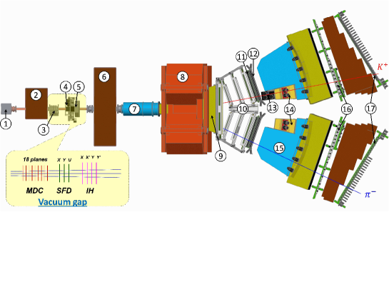
Figure 1: General view of the DIRAC setup: 1 – target station; 2 – first shielding; 3 – microdrift chambers; 4 – scintillating fiber detector; 5 – ionisation hodoscope; 6 – second shielding; 7 – vacuum tube; 8 – spectrometer magnet; 9 – vacuum chamber; 10 – drift chambers; 11 – vertical hodoscope; 12 – horizontal hodoscope; 13 – aerogel Cherenkov; 14 – heavy gas Cherenkov; 15 – nitrogen Cherenkov; 16 – preshower; 17 – muon detector.

After the target station primary protons run forward to the beam dump, and the secondary channel with the whole setup is vertically inclined relative to the proton beam by $5.7^{\circ}$ upward. Secondary particles are confined by the rectangular beam collimator inside of the second steel shielding wall, and the angular divergence in the horizontal (X) and vertical (Y) planes is $\pm 1^{\circ}$ and the solid angle $\Omega=1.2\cdot 10^{-3}$ sr. With a spill duration of 450 ms the beam intensity has been (10.5 – 12) $\cdot 10^{10}$ protons/spill and, correspondingly, the single counting rate in one plane of the ionisation hodoscope (IH) (5 – 6) $\cdot 10^{6}$ particles/spill. Secondary particles propagate mainly in vacuum up to the Al foil with a thickness of 0.68 mm $(7.6\cdot 10^{-3}X_{0})$ at the exit of the vacuum chamber, which is located between the poles of the dipole magnet ($B_{max}$ = 1.65 T and $BL$ = 2.2 Tm).

In the vacuum gap 18 planes of the MicroDrift Chambers (MDC) and 3 planes (X, Y, U) of the Scintillating Fiber Detector (SFD) have been installed to measure the particle coordinates ($\sigma_{SFDx}=\sigma_{SFDy}=60~{}\mu$m, $\sigma_{SFDu}=120~{}\mu$m) and the particle time ($\sigma_{tSFDx}=380$ ps, $\sigma_{tSFDy}=\sigma_{tSFDu}=520$ ps). The four IH planes serve to identify unresolved double tracks (signal only from one SFD column). The total matter radiation thickness between target and vacuum chamber amounts to $5.6\cdot 10^{-2}X_{0}$.

Each spectrometer arm is equipped with the following subdetectors [21]: drift chambers (DC) to measure particle coordinates with $\approx$85 $\mu$m precision; vertical hodoscope (VH) to measure time with 110 ps accuracy for particle identification via time-of-flight determination; horizontal hodoscope (HH) to select in the two arms particles with vertical distances less than 75 mm ($Q_{Y}$ less than 15 MeV/c); aerogel Cherenkov counter (ChA) to distinguish kaons from protons; heavy gas ($C_{4}F_{10}$) Cherenkov counter (ChF) to distinguish pions from kaons; nitrogen Cherenkov (ChN) and preshower (PSh) detector to identify $\mathrm{e}^{+}\mathrm{e}^{-}$ pairs; iron absorber; two-layer muon scintillation counter (Mu) to identify muons. In the “negative” arm no aerogel counter has been installed, because the number of antiprotons is small compared to $K^{-}$.

Pairs of oppositely charged particles, time-correlated (prompt pairs) and accidentals in the time interval $\pm 20$ ns, are selected by requiring a 2-arm coincidence (ChN in anticoincidence) with a coplanarity restriction (HH) in the first-level trigger. The second-level trigger selects events with at least one track in each arm by exploiting DC-wire information (track finder). Using track information the online trigger selects $\pi\pi$ and $\pi K$ pairs with $|Q_{X}|<12~{}\rm{MeV/c}$ and $|Q_{L}|<30~{}\rm{MeV/c}$ . The trigger efficiency is $\approx$ 98% for pairs with $|Q_{X}|<6~{}\rm{MeV/c}$, $|Q_{Y}|<4~{}\rm{MeV/c}$ and $|Q_{L}|<28~{}\rm{MeV/c}$. For spectrometer calibration $\pi^{-}p$ ($\pi^{+}\bar{p}$) pairs from $\Lambda$ ($\bar{\Lambda}$) decay have been investigated, and $\mathrm{e}^{+}\mathrm{e}^{-}$ pairs for general detector calibration.

3 Production of bound and free and $\pi^{-}K^{+}$ and $\pi^{+}K^{-}$ pairs

Prompt $\pi^{\mp}K^{\pm}$ pairs from proton-nucleus collisions are produced either directly or originate from short-lived (e.g. $\Delta$, $\rho$), medium-lived (e.g. $\omega$, $\phi$) or long-lived (e.g. $\eta^{\prime}$, $\eta$) sources. Pion-kaon pairs produced directly, from short- and medium-lived sources undergo Coulomb final state interaction (Coulomb pair in Fig. 2) and so may form bound states. Pairs from long-lived sources are practically not affected by Coulomb interaction (non-Coulomb pair in Fig. 2). The accidental pairs are produced in different proton-nucleus interactions.

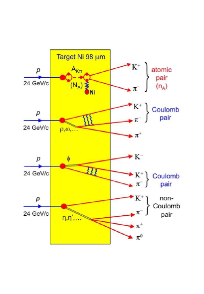
Figure 2: Inclusive $\pi K$ production in 24 GeV/c p-Ni interaction: p + Ni $\to$ $\pi^{\mp}K^{\pm}$ + X. The ionisation or breakup of $\pi K$ atoms, $A_{K\pi}$, leads to so-called atomic pairs. (More details, see text)

The cross section of $\pi K$ atom production is given by the expression [15]:

$$\frac{{\rm d}\sigma^{n}_{A}}{{\rm d}\vec{p}_{A}}=(2\pi)^{3}\frac{E_{A}}{M_{A}}\left.\frac{{\rm d}^{2}\sigma^{0}_{s}}{{\rm d}\vec{p}_{K}{\rm d}\vec{p}_{\pi}}\right|_{\frac{\vec{p}_{K}}{M_{K}}\approx\frac{\vec{p}_{\pi}}{M_{\pi}}}\cdot\left|\psi_{n}(0)\right|^{2}=(2\pi)^{3}\frac{E_{A}}{M_{A}}\frac{1}{\pi a_{B}^{3}n^{3}}\left.\frac{{\rm d}^{2}\sigma^{0}_{s}}{{\rm d}\vec{p}_{K}{\rm d}\vec{p}_{\pi}}\right|_{\frac{\vec{p}_{K}}{M_{K}}\approx\frac{\vec{p}_{\pi}}{M_{\pi}}}\>,$$ (4)

where $\vec{p}_{A}$, $E_{A}$ and $M_{A}$ are the momentum, total energy and mass of the $\pi K$ atom in the laboratory (lab) system, respectively, and $\vec{p}_{K}$ and $\vec{p}_{\pi}$ the momenta of the charged kaon and pion with equal velocities. Therefore, these momenta obey in good approximation the relations $\vec{p}_{K}=\frac{M_{K}}{M_{A}}\vec{p}_{A}$ and $\vec{p}_{\pi}=\frac{M_{\pi}}{M_{A}}\vec{p}_{A}$. The inclusive production cross section of $\pi K$ pairs from short-lived sources without final state interaction (FSI) is denoted by $\sigma_{s}^{0}$, and $\psi_{n}(0)$ is the $S$-state atomic wave function at the origin with principal quantum number $n$. According to (4) $\pi K$ atoms are only produced in $S$-states with probabilities $W_{n}~{}=~{}\frac{W_{1}}{n^{3}}$: $W_{1}~{}=~{}83.2\%$, $W_{2}~{}=~{}10.4\%$, $W_{3}~{}=~{}3.1\%$, $\dots$ , $W_{n>3}~{}=~{}3.3\%$.

In complete analogy, the production of free $\pi^{\mp}K^{\pm}$ pairs from short- and medium-lived sources, i.e. Coulomb pairs, is described in the pointlike production approximation in dependence of relative momentum $q$ (section 1) by

$$\frac{{\rm d}^{2}\sigma_{C}}{{\rm d}\vec{p}_{K}{\rm d}\vec{p}_{\pi}}=\frac{{\rm d}^{2}\sigma^{0}_{s}}{{\rm d}\vec{p}_{K}{\rm d}\vec{p}_{\pi}}\cdot A_{C}(q)\quad\mbox{with}\quad A_{C}(q)=\frac{4\pi\mu\alpha/q}{1-\exp\left(-4\pi\mu\alpha/q\right)}\;.$$ (5)

The Coulomb enhancement function $A_{C}(q)$ is the well-known Sommerfeld-Gamov-Sakharov factor [22, 23, 24].

The relative yield between atoms and Coulomb pairs [25] is given by the ratio of (4) to (5). The total number $N_{A}$ of produced $\pi K$ atoms is determined by the model-independent relation

$$N_{A}=k(q_{0})N_{C}(q\leq q_{0})\quad\mbox{with}\quad k(q_{0}=3.12~{}\rm{MeV/c})=0.615\>,$$ (6)

where $N_{C}(q\leq q_{0})$ is the number of Coulomb pairs with relative momenta $q\leq q_{0}$ and $k(q_{0})$ a known function of $q_{0}$. By using the Monte Carlo (MC) technique, one gets the same relationship as in (6), but this time in terms of the experimental relative momentum $Q$.

So far the pair production is assumed to be pointlike. In order to check for finite size effects due to the presence of medium-lived particles ($\omega$, $\phi$), a study of non-pointlike particle pair sources has been performed [26]. Due to the large value of the Bohr radius, $a_{B}=249$ fm, the pointlike treatment of the Coulomb $\pi K$ FSI is valid for directly produced pairs as well as for pairs from short-lived resonances. For $\pi$ and $K$ from medium-lived sources, corrections at the percent level have been applied to the production cross sections [26]. Strong final state elastic and inelastic $\pi K$ interactions are negligible.

4 Interaction of $\pi K$ and $\pi\pi$ atoms with matter

While propagating through the target material, relativistic $\pi K$ atoms can get excited or even ionised. The ionisation or breakup process competes with $\pi K$ atom annihilation. The breakup probability $P_{\text{br}}$ as a function of the atom lifetime $\tau$, atom momentum $p_{A}$, target material and thickness has been extensively studied in the pionium case. To guarantee knowledge of $P_{\text{br}}(\tau,p_{A})$ at the 1% level, one has to take into account a series of projectile collisions with matter atoms along the path in the target, leading to transitions between various bound states or to breakup. For $\pi\pi$ atoms the resulting system of equations is solved exactly by eigendecomposition of the corresponding matrix [27, 28] or by MC simulations [29]. The same approach can be applied for $\pi K$ atoms.

In the present paper we use a set of total and transition cross sections calculated in the first Born approximation for $\pi K$ atoms interacting with Ni atoms, according to the method described in [27]. Solving the equation system, the breakup probability $P_{\text{br}}(\tau)$ (Fig. 3) is obtained by convoluting $P_{\text{br}}(\tau,p_{A})$ with the experimental lab momentum spectra of small relative momentum $\pi K$ Coulomb pairs. The function $P_{\text{br}}(\tau)$ is used to extract a lifetime estimate from the measured $\pi K$ atom breakup probability.

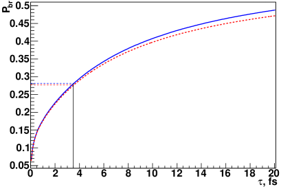
Figure 3: Probability of $\pi K$ atom breakup as a function of ground state lifetime $\tau$ in Ni targets of thicknesses $98\>\mu$m (Ni-1: dashed red) and $108\>\mu$m (Ni-2: solid blue). The predicted lifetime $\tau=3.5\cdot 10^{-15}$ s (Eq. 3) corresponds to the breakup probability $P_{\text{br}}$ = 0.28.

5 Data processing

Recorded events have been reconstructed with the DIRAC $\pi\pi$ [7] analysis software ARIANE [30] modified for analysing $\pi K$ data.

5.1 Tracking and setup tuning

Only events with one or two particle tracks in the DC of each arm are processed. Event reconstruction is performed according to the following steps: 1) One or two hadron tracks are identified in DC of each arm with hits in VH, HH and PSh slabs and no signal in ChN and Mu (Fig. 1). The earliest track in each arm is used for further analysis. 2) So-called DC tracks are extrapolated backward to the incident proton beam position on the target, using the transfer function of the DIRAC dipole magnet [31]. This procedure provides approximated particle momenta and corresponding intersection points in MDC, SFD and IH. 3) Hits are searched around the expected SFD coordinates in the region defined by position accuracy. For events with low and medium background, the number of hits around the two tracks is $\leq 4$ in each SFD plane and $\leq 9$ in all 3 SFD planes. These criteria reduce the data sample by 1/3. In order to find the best two-track combination, the momentum of the positive or negative particle may be modified to match the $X$-coordinates of tracks in DC and the SFD hits in the $X$- or $U$-plane. Furthermore, the two tracks may not use a common SFD hit in case of more than one hit in the proper region. In the final analysis the combination with the best $\chi^{2}$ in the other SFD planes is kept.

To check and align the setup components, we take advantage of the $\Lambda\to\pi^{-}{\rm p}$ and $\bar{\Lambda}\to\pi^{+}\bar{\rm p}$ decays [32, 33]. Using data from 2008 to 2010 and after geometrical alignment, the reconstructed $\Lambda$ mass [$(1.115685\pm 1.2\cdot 10^{-6})$ GeV/c²] agrees well with the PDG value [$(1.115683\pm 6\cdot 10^{-6})$ GeV/c²] [34, 35]. The width of the $\Lambda$ peak is a tool to evaluate the momentum resolution: it depends mainly on multiple scattering in the upstream setup part and in the Al membrane at the exit of the vacuum chamber as well as on DC resolution and alignment. The upstream multiple scattering has been determined by analysing $\pi\pi$ events [36]. The MC simulation underestimates the $\Lambda$ width by 6 – 7% with respect to the experimental value, and this difference is consistent for each momentum bin and for $\Lambda$ and $\overline{\Lambda}$. Hence we attribute the discrepancy between experiment and simulation to an imperfect description of the downstream setup part. To fix it, a Gaussian smearing of the reconstructed momenta is introduced. The smearing applied event-by-event is given by the formula: $p^{smeared}=p\;(1+C_{f}\cdot N(0,1))$, where $p$ is the reconstructed proton or pion momentum and $N(0,1)$ a random number generated according to the standard normal distribution. Smearing of simulated momenta with $C_{f}=(7\pm 4)\cdot 10^{-4}$ leads to a $\Lambda$ width in the reconstructed MC events consistent with experimental data [34] (Fig. 4).

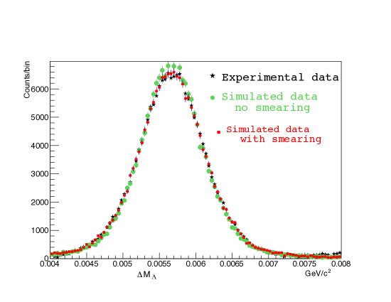
Figure 4: Invariant $\pi^{-}{\rm p}$ mass distribution in the $\Lambda$ region. [$\Delta{\rm M}_{\Lambda}={\rm M}_{\Lambda}-1.11$ GeV/c²; green: MC distribution without smearing; red: MC with smearing of $7\cdot 10^{-4}$; black: experimental data]

Using the decays $\Lambda\to\pi^{-}{\rm p}$ and $\bar{\Lambda}\to\pi^{+}\bar{\rm p}$ and taking into account momentum smearing, the momentum resolution has been evaluated as $\frac{dp}{p}=\frac{p_{gen}-p_{rec}}{p_{gen}}$ with $p_{gen}$ and $p_{rec}$ the generated and reconstructed momenta, respectively. Between 1.5 and 8 GeV/c DIRAC is able to reconstruct particle momenta with a relative precision from $2.8\cdot 10^{-3}$ to $4.4\cdot 10^{-3}$. The following resolutions in ($Q_{X}$, $Q_{Y}$, $Q_{L}$) after the target are obtained by MC simulation: $\sigma_{QX}\approx\sigma_{QY}\approx 0.18~{}\rm{MeV}/c$, $\sigma_{QL}\approx 0.85~{}{\rm MeV}/c$ for $p_{\pi K}=p_{\pi}+p_{K}=5$ GeV/c and about 6% higher values for $p_{\pi K}=7.5$ GeV/c.

5.2 Event selection

Selected events are divided into the categories $\pi^{-}K^{+}$, $\pi^{+}K^{-}$ and $\pi^{+}\pi^{-}$. The last event type is used for calibration purposes. Pairs of $\pi K$ are cleaned from $\pi^{+}\pi^{-}$, $\pi^{-}{\rm p}$ and $\pi^{+}\bar{\rm p}$ background by the Cherenkov counters ChF and ChA. In the momentum range from 3.8 to 7 GeV/c pions are detected by ChF with (95 – 97)% efficiency [37], whereas kaons and protons (antiprotons) do not produce a signal. The admixture of $\pi^{-}{\rm p}$ pairs is suppressed by the aerogel Cherenkov detector (ChA), which records kaons but not protons [38]. By requiring a signal in ChA and selecting compatible time-of-flights between target and VH, $\pi^{-}{\rm p}$ and $\pi^{-}\pi^{+}$ pairs, contaminating $\pi^{-}K^{+}$, can be substantially suppressed. Fig. 6 shows the well-defined $\pi^{-}K^{+}$ Coulomb peak at $Q_{L}=0$ and the strongly suppressed peak from $\Lambda$ decays at $Q_{L}=-30$ MeV/c. Similarly Fig. 6 presents the $\pi^{+}K^{-}$ Coulomb peak at $Q_{L}=0$ and a second weaker peak from $\overline{\Lambda}$ decay at $Q_{L}=30$ MeV/c .

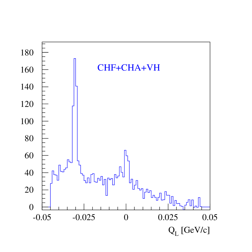
Figure 5: $Q_{L}$ distribution of hypothesised $\pi^{-}K^{+}$ pairs after applying the selection described in the text. Events with positive $Q_{L}$ are suppressed compared to those with negative $Q_{L}$ due to lower acceptance and lower production cross section.

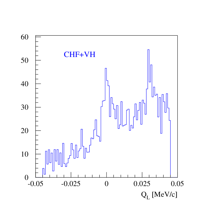
Figure 6: $Q_{L}$ distribution of hypothesised $\pi^{+}K^{-}$ pairs after selection. Events with negative $Q_{L}$ are suppressed compared to those with positive $Q_{L}$ due to acceptance and cross section.

The final analysis sample contains only events which fulfil the following criteria:

$$|Q_{X}|<6~{}{\rm MeV/c}\,,\,|Q_{Y}|<4~{}{\rm MeV/c}\,,\,|Q_{L}|<15~{}{\rm MeV/c}\,.$$ (7)

Due to finite detector efficiency still a certain admixture of misidentified pairs remains in the experimental distribution. Their contribution has been estimated by time-of-flight investigations and accordingly subtracted [39].

6 Data simulation

Since the $\pi K$ data samples consist of Coulomb, non-Coulomb and atomic pairs, three event types have been generated by MC in adequate high statistics. These events are characterised by different $q$ distributions: the non-Coulomb pairs are uniformly distributed in low $q$, while the $q$ distribution for Coulomb pairs is modified by the factor $A_{C}(q)$ (Eq. 5). For each atomic pair one needs to know the position of the breakup and the lab momentum. In practice the MC lab momentum distributions are approximated by analytic formulae, which resemble the experimental momentum distributions of such pairs [40, 41]. After comparing experimental momentum spectra [39] with MC distributions reconstructed by the analysis software, the simulated distributions have been fitted to the experimental data by a weight function. The breakup point and the quantum numbers of the atomic state, from which ionisation occurred, are obtained by solving numerically the transport equations [28], using total and transition cross sections [27]. The lab momenta of the atoms are assumed to be the same as for Coulomb pairs. The description of the charged particle propagation through the setup takes into account: a) multiple scattering in the target, detector planes and partitions, b) response of all detectors, c) additional smearing of particle momentum, d) results of SFD response analysis [42, 43, 39] with influence on the $Q_{T}$ resolution.

7 Data analysis

The analysis of $\pi K$ data is similar to that of $\pi^{+}\pi^{-}$ data [7]: experimental distributions of relative momentum $Q$ components have been fitted by simulated distributions of atomic, Coulomb and non-Coulomb pairs. Their corresponding numbers $n_{A}$, $N_{C}$ and $N_{nC}$ are free fit parameters. The relation (6) between the numbers of produced atoms and Coulomb pairs allows to derive the breakup probability. The same procedure has been applied to $\pi^{-}K^{+}$ (Fig. 7) and $\pi^{+}K^{-}$ (Fig. 8) pairs. The $Q_{L}$ distributions shown are obtained from the 2-dimensional ($Q_{T},Q_{L}$) distributions in the region $Q_{T}<4~{}$ MeV/c, $|Q_{L}|<15$ MeV/c for pairs with lab momenta $4.8<p_{\pi^{-}}+p_{K^{+}}<7.2$ GeV/c and $4.8<p_{\pi^{+}}+p_{K^{-}}<7.6$ GeV/c. The different background conditions are taken into account. One observes an excess of events in Fig. 7 and 8 in the low $Q_{L}$ region, where atomic pairs are expected.

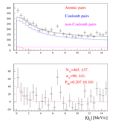
Figure 7: Top: Experimental $|Q_{L}|$ distribution of $\pi^{-}K^{+}$ pairs [2-dimensional ($Q_{T},Q_{L}$) analysis] fitted by the sum of simulated distributions of atomic, Coulomb and non-Coulomb pairs. Atomic pairs are shown in red, and free pairs (Coulomb and non-Coulomb) in black. Bottom: Difference distribution between experimental and simulated free pair distributions compared with simulated atomic pairs.

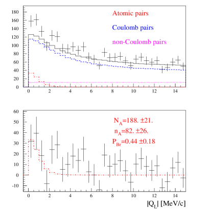
Figure 8: Experimental $|Q_{L}|$ distributions for $\pi^{+}K^{-}$ pairs analogous to Fig. 7.

Similarly the analysis has been performed for the 1-dimensional ($Q_{L}$) distributions with the results shown in Table 1. The 1- and 2-dimensional distributions have different sensitivities to sources of systematic errors [44]. Comparing the two outcomes allows to check the stability of our analysis procedure. The experimental conditions vary from 2008 to 2010 due to setup updates and beam quality. Table 1 summarises all the fit results of the data samples analysed on the basis of the 2-dimensional as well as the 1-dimensional distributions. The number of reconstructed atomic pairs of both charge combinations from the 2-dimensional analysis amounts to $n_{A}(\pi^{-}K^{+}+\pi^{+}K^{-})=178\pm 49$ (3.6 sigma). On the basis of this number the extracted values for the breakup probability presented in the last column of Table 1 provide a means to estimate the $\pi K$ atom lifetime.

Table 1: Results for $N_{A}$ (number of produced atoms), $n_{A}$ (number of atomic pairs) and $P_{br}$ (breakup probability) by analysing 2-dimensional ($Q_{T},Q_{L}$) and 1-dimensional ($Q_{L}$) distributions.

Year	$N_{A}$	$n_{A}$	$P_{br}$
$\pi^{-}K^{+}$ over $Q_{T},Q_{L}$
2008	$132\pm 16$	$14\pm 19$	$0.11\pm 0.15$
2009	$169\pm 24$	$33\pm 26$	$0.20\pm 0.17$
2010	$164\pm 23$	$49\pm 26$	$0.30\pm 0.19$
$\pi^{-}K^{+}$ over $Q_{L}$
2008	$125\pm 19$	$25\pm 30$	$0.20\pm 0.26$
2009	$151\pm 28$	$54\pm 42$	$0.36\pm 0.33$
2010	$155\pm 28$	$61\pm 42$	$0.39\pm 0.32$
$\pi^{+}K^{-}$ over $Q_{T},Q_{L}$
2008	$51\pm 11$	$21\pm 13$	$0.41\pm 0.33$
2009	$77\pm 13$	$26\pm 16$	$0.34\pm 0.24$
2010	$60\pm 12$	$35\pm 16$	$0.58\pm 0.36$
$\pi^{+}K^{-}$ over $Q_{L}$
2008	$47\pm 13$	$35\pm 21$	$0.75\pm 0.62$
2009	$76\pm 15$	$28\pm 24$	$0.37\pm 0.37$
2010	$83\pm 15$	$-4\pm 22$	$-0.04\pm 0.26$

8 Systematic errors

The evaluation of the breakup probability $P_{\text{br}}$ is affected by several sources of systematic errors [39]. Most of them are induced by imperfections in the simulation of the different $\pi K$ pairs: atomic, Coulomb, non-Coulomb and misidentified pairs. Shape differences of experimental and simulated distributions in the fit procedure (section 7) lead to biases on parameters, including breakup probability. The influence of error sources is different for the ($Q_{T},Q_{L}$) and $Q_{L}$ analyses. Table 2 shows systematic errors common to $\pi^{-}K^{+}$ and $\pi^{+}K^{-}$ collected from 2008 to 2010.

Table 2: Systematic errors in $P_{\text{br}}$ common to all data collected from 2008 to 2010.

Sources of systematic errors	$\sigma^{syst}_{Q_{T},Q_{L}}$	$\sigma^{syst}_{Q_{L}}$
Uncertainty in $\Lambda$ width correction	0.005	0.0015
Accuracy of SFD simulation	0.0008	0.0003
Correction of Coulomb correlation function on finite size production region	0.00006	0.00006
Uncertainty in $P_{br}(\tau)$ dependence	0.005	0.005
Uncertainty in target thickness	0.0003	$<0.0003$

Other sources of systematic errors are uncertainties in the measuring procedure for $\pi K$ and background distributions. These spectra have been measured individually for the different run periods, producing systematic errors $\sigma^{syst}_{\pi K}$ and $\sigma^{syst}_{back}$ in $P_{br}$ (see Table 3). The presented systematic errors have been included in estimating the $\pi K$ atom lifetime as described in the next section.

Table 3: Systematic errors in $P_{\text{br}}$ specific to the data samples collected in 2008, 2009 and 2010.

Year	$\sigma^{syst}_{\pi K}$	$\sigma^{syst}_{back}$
$K^{+}\pi^{-}$ over $Q_{T},Q_{L}$
2008	0.0028	0.0015
2009	0.0044	0.0025
2010	0.0036	0.0022
$K^{+}\pi^{-}$ over $Q_{L}$
2008	0.0030	0.0028
2009	0.0053	0.0044
2010	0.0046	0.0036
$\pi^{+}K^{-}$ over $Q_{T},Q_{L}$
2008	0.0072	0.0067
2009	0.0048	0.0028
2010	0.0017	0.0043
$\pi^{+}K^{-}$ over $Q_{L}$
2008	0.0093	0.0072
2009	0.0047	0.0048
2010	0.0021	0.0017

9 Lifetime and scattering length measurements

The lifetime dependence of the breakup probability $P_{\text{br}}(\tau,p_{A})$ for $\pi^{\mp}K^{\pm}$ atoms with momentum $p_{A}$ has been determined [28], using total and excitation cross sections calculated in Born approximation [27]. Convoluting $P_{\text{br}}(\tau,p_{A})$ with the corresponding lab momentum spectra (section 4 and [39]) leads to a set of $P_{\text{br},i}(\tau)$ functions, each for every target thickness (Ni-1, Ni-2) and experimental spectrum ($\pi^{+}K^{-}$, $\pi^{-}K^{+}$). To estimate the ground state lifetime the maximum likelihood method [45] has been applied:

$$L(\tau)=\exp\left(-U^{T}G^{-1}U/2\right),$$ (8)

where $U$ with $U_{i}=\Pi_{i}-P_{\text{br},i}(\tau)$ is a vector of differences between measured $\Pi_{i}$ ($P_{br}$ in Table 1) and theoretical breakup probability $P_{\text{br},i}(\tau)$ for data sample $i$. The matrix $G$, the error matrix of $U$, includes statistical and systematic uncertainties (Table 2 and 3):

$$G_{ij}=\delta_{ij}\left[(\sigma^{\text{stat}}_{i})^{2}+(\sigma^{\text{syst}}_{\pi K,i})^{2}+(\sigma^{\text{syst}}_{\text{back},i})^{2}\right]+(\sigma^{\text{syst}}_{\text{global}})^{2}.$$ (9)

By combining the two charge combinations ($\pi^{\mp}K^{\pm}$) and considering the statistics collected from 2008 to 2010, the $(Q_{T},Q_{L})$ analysis yields the following ground state lifetime estimation:

$$\tau=\left.\left.(2.5_{-1.8}^{+3.0}\right|_{\text{stat}}{}_{-0.1}^{+0.3}\right|_{\text{syst}}\>)\text{fs}=\left.(2.5_{-1.8}^{+3.0}\right|_{\text{tot}}\>)\text{fs}.$$ (10)

This experimental value agrees with the predicted one of Eq. (3).

The estimated ground state lifetime (10) corresponds to the $\pi K$ scattering length (1)

$$\left|a_{0}^{-}\right|M_{\pi}=\frac{1}{3}\left|a_{1/2}-a_{3/2}\right|M_{\pi}=0.107_{-0.035}^{+0.093}=0.11_{-0.04}^{+0.09}\>,$$ (11)

to be compared with the theoretical predictions (2).

The $Q_{L}$ analysis (Table 1, 2 and 3) provides a similar estimation of the ground state lifetime, but with worse precision:

$$\tau=\left.\left.(2.4_{-2.2}^{+5.4}\right|_{\text{stat}}{}_{-0.1}^{+0.5}\right|_{\text{syst}}\>)\text{fs}=\left.(2.4_{-2.2}^{+5.5}\right|_{\text{tot}}\>)\text{fs}.$$ (12)

10 Conclusion

The analysis of $\pi K$ pairs collected from 2008 to 2010 allows to evaluate the number of atomic $\pi K$ pairs ($178\pm 49$) as well as the number of produced $\pi K$ atoms ($653\pm 42$) and thus the breakup (ionisation) probability. By exploiting the dependence of breakup probability on atom lifetime, a value for the $\pi K$ atom 1S lifetime $\tau=(2.5_{-1.8}^{+3.0})$ fs has been extracted. As the atom lifetime is related to a scattering length, a measurement of the S-wave isospin-odd $\pi K$ scattering length $\left|a_{0}^{-}\right|=\left(0.11_{-0.04}^{+0.09}\right)M_{\pi}^{-1}$ can be presented, compatible with theory.

References

- [1] S. Weinberg, Phys. Rev. Lett. 17 (1966) 616.
- [2] J. Gasser, H. Leutwyler, Nucl. Phys. B250 (1985) 465.
- [3] B. Moussallam, Eur. Phys. J. C14 (2000) 111.
- [4] G. Colangelo, J. Gasser, H. Leutwyler, Nucl. Phys. B603 (2001) 125.
- [5] L. Afanasyev et al., Phys. Lett. B338 (1994) 478.
- [6] B. Adeva et al., Phys. Lett. B619 (2005) 50.
- [7] B. Adeva et al., Phys. Lett. B704 (2011) 24.
- [8] S.M. Bilen’kii et al., Yad. Fiz. 10 (1969) 812; (Sov. J. Nucl. Phys. 10 (1969) 469).
- [9] J. Schweizer, Phys. Lett. B587 (2004) 33.
-
[10]
V. Bernard, N. Kaiser, U.-G. Meissner, Phys. Rev. D43 (1991) 2757;
Nucl. Phys. B357 (1991) 129. - [11] B. Kubis, U.G. Meissner, Phys. Lett. B529 (2002) 69.
- [12] J. Bijnens, P. Dhonte, P. Talavera, JHEP 0405 (2004) 036.
- [13] P. Buettiker, S. Descotes-Genon, B. Moussallam, Eur. Phys. J. C33 (2004) 409.
- [14] C.B. Lang et al., arXiv:1207.3204 [hep-lat].
- [15] L.L. Nemenov, Yad. Fiz. 41 (1985) 980; (Sov. J. Nucl. Phys. 41 (1985) 629).
- [16] O.E. Gorchakov et al., Yad. Fiz. 63 (2000) 1936; (Phys. At. Nucl. 63 (2000) 1847).
- [17] Y. Allkofer, PhD thesis, Universität Zürich, 2008.
- [18] B. Adeva et al., Phys. Lett. B674 (2009) 11.
- [19] O.E. Gorchakov, A. Kuptsov, DN555DN=DIRAC-NOTE-2005-05 (cds.cern.ch/record/1369686).
- [20] O. Gorchakov, DN-2005-23 (cds.cern.ch/record/1369668).
-
[21]
B. Adeva et al.,
Updated CERN DIRAC spectrometer for dimeson atom investigation,
to be submitted to Nucl. Instrum. Meth. - [22] A. Sommerfeld, Atombau und Spektrallinien, F. Vieweg & Sohn (1931).
- [23] G. Gamov, Z. Phys. 51 (1928) 204.
-
[24]
A. Sakharov, Zh. Eksp. Teor. Fiz. 18 (1948) 631;
Sov. Phys. Usp. 34 (1991) 375. - [25] L. Afanasyev, O. Voskresenskaya, Phys. Lett. B453 (1999) 302.
- [26] R. Lednicky, J. Phys. G: Nucl. Part. Phys. 35 (2008) 125109.
- [27] L. Afanasyev, A. Tarasov, Phys. At. Nucl. 59 (1996) 2130.
- [28] M. Zhabitsky, Phys. At. Nucl. 71 (2008) 1040.
- [29] C. Santamarina et al., J. Phys. B36 (2003) 4273.
-
[30]
D. Drijard, M. Hansroul, V. Yazkov, DIRAC offline user guide
(dirac.web.cern.ch/DIRAC/offlinedocs/Userguide.html). - [31] O. Gorchakov, DN-2009-04 (cds.cern.ch/record/1369631).
- [32] O. Gortchakov, DN-2009-10, 2009-02 (cds.cern.ch/record/1369625, 1369633).
- [33] B. Adeva, A. Romero, O. Vazquez Doce, DN-2005-16 (cds.cern.ch/record/1369675).
- [34] A. Benelli, V. Yazkov, DN-2013-03 (cds.cern.ch/record/1622175).
- [35] J. Beringer et al. (Particle Data Group), Phys. Rev. D86, 010001 (2012)
- [36] A. Benelli, V. Yazkov, DN-2012-04 (cds.cern.ch/record/1475780).
- [37] P. Doskarova, V. Yazkov, DN-2013-05 (cds.cern.ch/record/1628541).
- [38] A. Benelli, V. Yazkov, DN-2009-07 (cds.cern.ch/record/1369628).
- [39] V. Yazkov, M. Zhabitsky, DN-2013-06 (cds.cern.ch/record/1628544).
- [40] O. Gorchakov, DN-2010-01 (cds.cern.ch/record/1369624).
- [41] M.V. Zhabitsky, DN-2007-11 (cds.cern.ch/record/1369651).
- [42] A. Gorin et al., Nucl. Instrum. Meth. A566 (2006) 500.
- [43] A. Benelli, SFD study and simulation for the data 2008-2010, DIRAC-TALK-2011-01.
- [44] V. Yazkov, DN-2008-04 (cds.cern.ch/record/1369641).
- [45] D. Drijard, M. Zhabitsky, DN-2008-07 (cds.cern.ch/record/1367888).