Substellar Objects in Nearby Young Clusters (SONYC) VIII: Substellar population in Lupus 3

Abstract

SONYC – Substellar Objects in Nearby Young Clusters – is a survey programme to investigate the frequency and properties of substellar objects in nearby star-forming regions. We present a new imaging and spectroscopic survey conducted in the young ($\sim 1\,$Myr), nearby ($\sim 200\,$pc) star-forming region Lupus 3. Deep optical and near-infrared images were obtained with MOSAIC-II and NEWFIRM at the CTIO-4m telescope, covering $\sim 1.4\,$deg² on the sky. The $i$-band completeness limit of 20.3 mag is equivalent to $0.009-0.02$ M_⊙, for A${}_{V}\leq 5$. Photometry and $11-12\,$yr baseline proper motions were used to select candidate low-mass members of Lupus 3. We performed spectroscopic follow-up of 123 candidates, using VIMOS at the Very Large Telescope (VLT), and identify 7 probable members, among which 4 have spectral type later than M6.0 and $T_{\mathrm{eff}}\leq 3000\,$K, i.e. are probably substellar in nature. Two of the new probable members of Lupus 3 appear underluminous for their spectral class and exhibit emission line spectrum with strong H_α or forbidden lines associated with active accretion. We derive a relation between the spectral type and effective temperature: T${}_{\mathrm{eff}}=(4120\pm 175)-(172\pm 26)\times\mathrm{SpT}$, where SpT refers to the M spectral subtype between 1 and 9. Combining our results with the previous works on Lupus 3, we show that the spectral type distribution is consistent with that in other star forming regions, as well as is the derived star-to-BD ratio of $2.0-3.3$. We compile a census of all spectroscopically confirmed low-mass members with spectral type M0 or later.

1 Introduction

SONYC - short for Substellar Objects in Nearby Young Clusters - is a comprehensive project aiming to provide a complete, unbiased census of substellar population down to a few Jupiter masses in young star forming regions. Studies of the substellar mass regime at young ages are crucial to understand the mass dependence in the formation and early evolution of stars and planets. Although the low-mass end of the Initial Mass Function (IMF) has been the subject of intensive investigation over more than a decade, and by various groups, its origin is still a matter of debate (e.g. Bonnell et al. 2007; Bastian et al. 2010; Jeffries 2012). The relative importance of several proposed processes (dynamical interactions, fragmentation, accretion, photoevaporation) responsible for the formation of brown dwarfs (BDs) is not yet clear.

The SONYC survey is based on extremely deep optical- and near-infrared wide-field imaging, combined with the Two Micron All Sky Survey (2MASS) and $Spitzer$ photometry catalogs, which are correlated to create catalogs of substellar candidates and used to identify targets for extensive spectroscopic follow-up. In this work for the first time we also include a proper motion analysis, which greatly facilitates the candidate selection. Our observations are designed to reach mass limits well below 0.01 M_⊙, and the main candidate selection method is based on the optical photometry. This way we ensure to obtain a realistic picture of the substellar population in each of the studied cluster, avoiding the biases introduced by the mid-infrared selection (only objects with disks), or methane-imaging (only T-dwarfs). So far we have published results for three regions: NGC 1333 (Scholz et al., 2009, 2012b, 2012a), $\rho$ Ophiuchi (Geers et al., 2011; Mužić et al., 2012), and Chamaeleon-I (Mužić et al., 2011). We have identified and characterized more than 50 new substellar objects, among them a handful of objects with masses close to, or below the Deuterium burning limit. Thanks to the SONYC survey and the efforts of other groups, the substellar IMF is now well characterized down to $\sim 5-10$M_J, and we find that the ratio of the number of stars with respect to brown dwarfs lies between 2 and 6. In NGC1333 we find that, down to $\sim 5$M_J, the free-floating objects with planetary masses

In this paper we present the SONYC campaign in the Lupus 3 star forming region. The Lupus dark cloud complex is located in the Scorpius-Centaurus OB association and consists of several loosely connected dark clouds showing different levels of star-formation activity (see Comerón 2008 for a detailed overview). The main site of star formation within the complex is Lupus 3, which contains one of the richest associations of T-Tauri stars (Schwartz, 1977; Krautter et al., 1997). The center of Lupus 3 is dominated by the two most massive members of the entire complex, the two Herbig Ae/Be stars known as HR 5999 and HR 6000. More than half of the known Lupus 3 members are found in the $0.3\times 0.3$ pc² area surrounding the pair (Nakajima et al., 2000; Comerón, 2008).

The low-mass (sub-)stellar content of Lupus 3 was extensively investigated using the data from the Spitzer Space Telescope. Merín et al. (2008) compiled the most complete census of stars and brown dwarfs in Lupus 3 at the time, using the data from their survey, together with the results of previous surveys by Nakajima et al. (2000); Comerón et al. (2003); Comerón (2008); López Martí et al. (2005); Allers et al. (2006); Allen et al. (2007); Chapman et al. (2007); Tachihara et al. (2007); Merín et al. (2007); Strauss et al. (1992); Gondoin (2006). Spectroscopic follow-up in the optical (FLAMES/VLT) by Mortier et al. (2011) confirmed the effectiveness of MIR-excess selection from Merín et al. (2008), with about 80% of the 46 observed sources confirmed as members of Lupus 3. Two wide-area photometric surveys in Lupus were conducted using the Wide Field Imager (WFI) at the La Silla 2.2-m telescope. López Martí et al. (2005) identified 22 new low-mass member candidates in an area of 1.6 deg² in Lupus 3, with about half of the candidates confirmed spectroscopically in surveys by Allen et al. (2007) and Mortier et al. (2011). Comerón et al. (2009) surveyed an area of more than 6 deg² in the Lupus 1, 3, and 4 clouds and identified $\sim$70 new candidate members of Lupus 3. About 50% of the photometric sample was revealed to belong to a background population of giant stars in a follow-up spectroscopic study by Comerón et al. (2013). The deepest survey so far in Lupus 3 (Comerón, 2011), did not report any brown dwarfs, despite the sensitivity to objects with sub-Jupiter masses. However, the surveyed area of $\sim 7^{\prime}\times 7^{\prime}$ was very small compared to the total extent of the cluster, and thus contained only a minor fraction of the total population. The substellar population in Lupus 3 remains therefore poorly constrained.

The distance to the Lupus star forming region is still a matter of debate, with the distance determinations from different studies ranging from 140 pc to 240 pc (Comerón, 2008). A widely-used value of $140\pm 20\,$ pc was derived by Hughes et al. (1993) using photometry and spectroscopy of F-G field stars in Lupus. Using an improved version of the same method, Lombardi et al. (2008) obtained a distance of $155\pm 8\,$ pc, but also suggest that the apparent thickness of Lupus might be the result of different Lupus sub-clouds being at different distances. Distances obtained from the moving-cluster method (Makarov, 2007) suggest a thickness of $\sim 80\,$pc, and places Lupus 3 at a distance of about 170 pc, or 25 pc farther than the center of the greater association. This spatial arrangement is in general agreement with the distances derived from Hipparcos parallaxes of individual stars located in different sub-clouds (Wichmann et al., 1998; Bertout et al., 1999). As pointed out by Comerón (2008), while a distance of 150 pc seems adequate for most of the clouds of the complex, a value of 200 pc is likely to be more appropriate for Lupus 3. We therefore adopt a distance of 200 pc throughout the analysis presented in this paper. Adopting the distance of 200 pc, and evolutionary tracks of Baraffe et al. (1998), Comerón et al. (2003) derive an age of 1-1.5 Myr for most of their observed members.

In this work we present new observations of the Lupus 3 cloud using the MOSAIC-II optical imager and NEWFIRM near-infrared imager at the CTIO-4m telescope. Observations and data reduction are explained in Section 2. Photometry, proper motions and criteria for candidate selection are presented in Section 3, and the spectral analysis in Section 4. The results are discussed in Section 5. Finally, we summarize the main conclusions in Section 6.

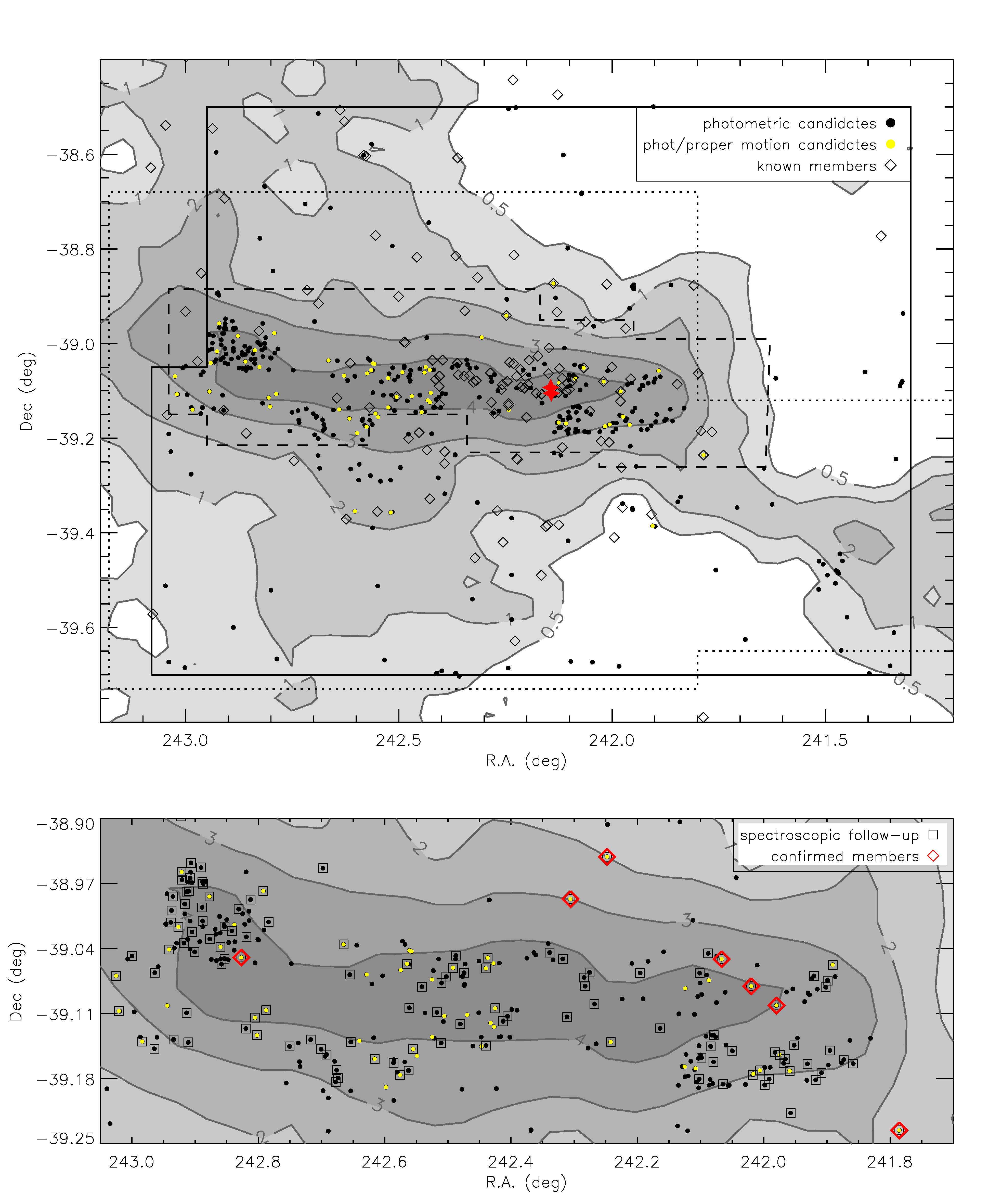
Figure 1: Upper panel: Spatial distribution of the candidate sources in Lupus 3. Photometric candidates are shown as black dots, those also selected by proper motions are shown in yellow. Diamonds mark previously known members, with the two red stars marking the brightest pair, HR5999/6000. Solid line shows the field-of-view of our optical and near-infrared survey, and the dotted line the extent of the WFI field used as the first epoch for the proper motions. The dashed lines indicate the region within which the VIMOS spectroscopic fields have been arranged. The shaded contours indicate A_V from the extinction map by Cambrésy (1999). Lower panel: Zoom into the region covered by spectroscopy. All the candidates observed in our follow-up are marked with squares, and the confirmed objects are represented by red diamonds.

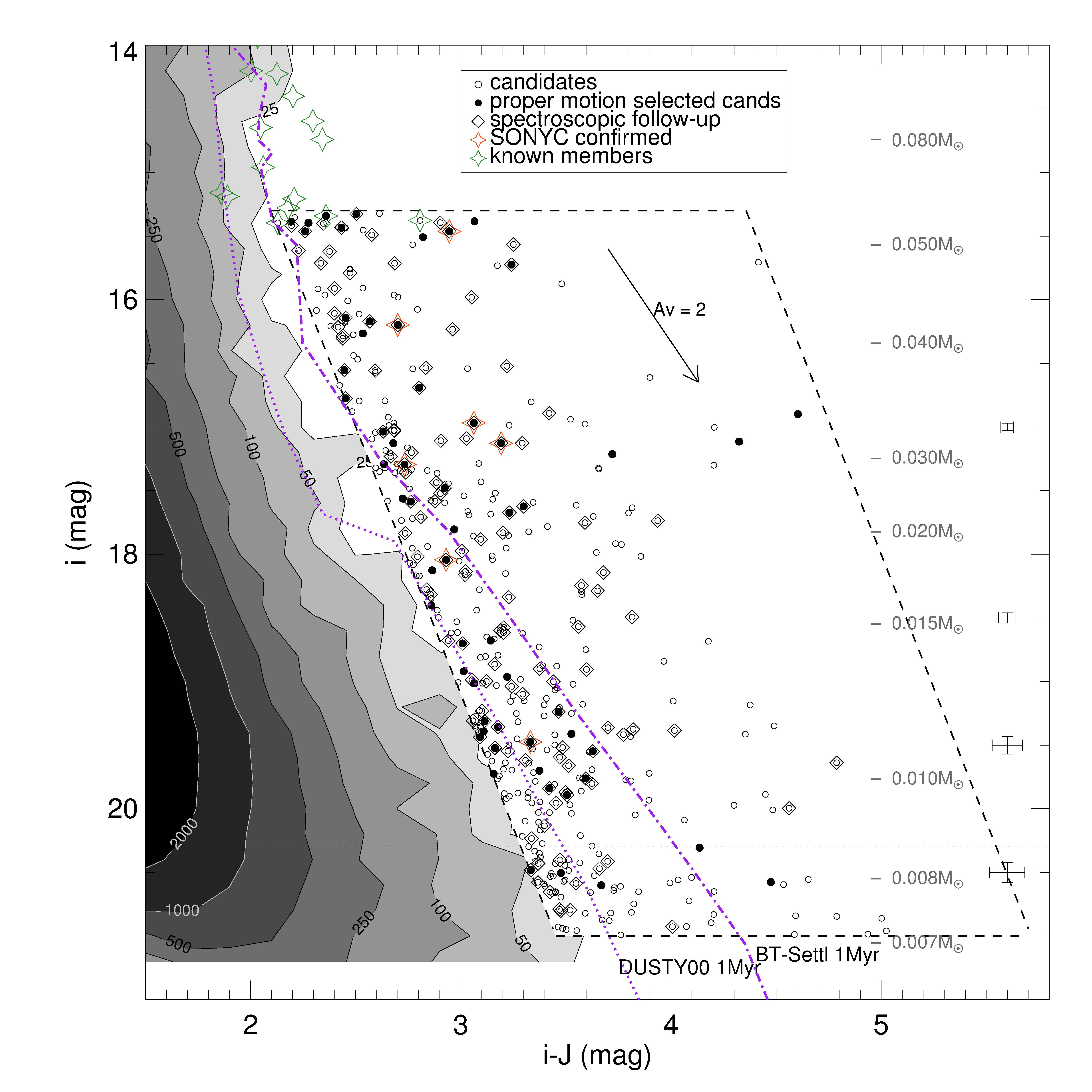
Figure 2: ($i$,$i-J$) color-magnitude diagram. Open circles represent all the photometrically-selected candidates located inside the selection box (dashed lines), with those additionally selected on the basis of their proper motions shown as filled circles. Diamonds show SONYC spectroscopy follow-up targets, with spectroscopically confirmed VLMOs highlighted as red (identified in this work) and green (previously known members) stars. Atmosphere model isochrones for age 1 Myr are overplotted for DUSTY00 (Chabrier et al., 2000) and BT-Settl (Allard et al., 2011). For clarity, the sources outside the candidate selection box are represented with contours, where the number on each contour represents the number of sources within a 0.2 mag $\times$ 0.2 mag bin. On the right-hand side of the figure we show 1$\sigma$ uncertainties of the photometry. The dotted line shows the completeness limit of our survey.

2 Observations and Data Reduction

2.1 Optical imaging

The imaging in the $i$-band was conducted using the MOSAIC-II CCD imager at the CTIO 4-meter telescope in Chile. MOSAIC-II is a wide-field imager with 8 CCDs arranged in a $4\times 2$ array. It provides a field of view of 36$\farcm$8 on a side, with a pixel scale of $0\farcs 27$ per pixel. We observed four pointings arranged around the two bright Herbig Ae/Be stars. The details of the observing run are summarized in Table 1, and the observed field is shown in Figure 1.

We reduced the MOSAIC-II images using tools in the $mscred$ package within IRAF. $Mscred$ contains the standard reduction tasks for CCD images, but adapted for the use on multi-chip mosaics. Series of dark frames and dome flats were combined to build an average zero and flatfield image. The zero and flatfield correction of the science mosaics was then carried out using the task ’ccdproc’. This also includes the subtraction of the bias level, derived from unexposed areas of the chip. For each of the four fields, the total integration time was split in a series of 24 exposures. To coadd these exposures, we first derived matching coordinate systems for all of them, using a list of USNO-A2 stars (obtained from Vizier) as reference. The frames were then matched and stacked using the tasks ’mscimage’ and ’mscstack’. Apart from a small region close to the center of the mosaic, which was excluded, this matching algorithm produces very good results. Note that the depth of the mosaics is not constant due to the small gaps between the detectors.

Photometry on the stacked images was carried out using ’daophot’ tools within IRAF. After generating a source catalogue with ’daofind’, the magnitudes were measured within a fixed aperture radius of 10 pixels using ’phot’. The sky background was estimated from an annulus with inner/outer radius of 10/15 pixels. To calibrate the $i$-band photometry we compared our instrumental magnitudes with the magnitudes of sources with $14.5<i<17.0$ in Lupus 3 from the Deep Near Infrared Survey catalog (DENIS; Epchtein et al. 1994), which used a Gunn $i$ filter centered at 0.8$\,\mu$m. For each field we calculate a zero point and apply it to all sources to create a final $i$-band catalog. The color-dependence of the calibration was investigated by calculating a coefficient $a$ in the color-term a$\times(i-J)$, which typically gives a$\sim$0.002. Its effect on photometry would be much smaller than the involved photometric uncertainties, and therefore it was not taken into account. Photometric uncertainties combine the errors returned by ’daophot’, with the errors of the photometric calibration. Typical photometric uncertainties are 0.05 mag at $i=19$ and 0.1 at $i=21$. The completeness limit of the deep exposures is $i\sim$20.3, with the magnitude range of $\sim$15.3 - 22.

For the proper motion calculation (see Section 3.2) we also used the $I_{C}$-band data obtained with the Wide Field Imager (WFI) at the MPI-ESO 2.2-m telescope at La Silla Observatory (Baade et al., 1999), that were previously published in López Martí et al. (2005). We therefore refer the reader to that paper for a detailed description of the data reduction procedures. The field observed with WFI is outlined with dotted line in Figure 1.

Table 1: Observing log for our imaging and spectroscopic surveys.

field #	$\alpha$(J2000)	$\delta$(J2000)	filter/grism	UT date	on-source time	instrument
Imaging
1	16:10:10	-38:49:08	$i$	12 06 2010	8100 s	MOSAIC-II
2	16:06:53	-38:49:37	$i$	12 06 2010	6900 s	MOSAIC-II
3	16:10:33	-39:22:34	$i$	13 06 2010	7500 s	MOSAIC-II
4	16:06:56	-39:22:16	$i$	13 06 2010	9000 s	MOSAIC-II
1	16:11:01	-38:38:20	$J$, $K_{S}$	15 06 2010, 16 06 2010	450 s, 400 s	NEWFIRM
2	16:08:39	-38:38:20	$J$, $K_{S}$	15 06 2010, 16 06 2010	450 s, 400 s	NEWFIRM
3	16:06:18	-38:38:20	$J$, $K_{S}$	15 06 2010, 05 05 2011	450 s, 420 s	NEWFIRM
4	16:11:01	-39:05:56	$J$, $K_{S}$	15 06 2010, 05 05 2011	450 s, 400 s	NEWFIRM
5	16:08:39	-39:05:56	$J$, $K_{S}$	15 06 2010, 05 05 2011	480 s, 460 s	NEWFIRM
6	16:06:18	-39:05:56	$J$, $K_{S}$	15 06 2010, 05 05 2011	450 s, 420 s	NEWFIRM
7	16:11:01	-39:33:32	$J$, $K_{S}$	15 06 2010, 05 05 2011	450 s, 440 s	NEWFIRM
8	16:08:39	-39:33:32	$J$, $K_{S}$	15 06 2010, 05 05 2011	450 s, 440 s	NEWFIRM
9	16:06:39	-39:33:32	$J$, $K_{S}$	15 06 2010, 05 05 2011	450 s, 460 s	NEWFIRM
Spectroscopy
1	16:11:24	-39:01:12	LR_red	26 06 2011	3500 s	VIMOS
2	16:11:18	-39:01:12	LR_red	12 06 2012	3500 s	VIMOS
3	16:11:00	-39:04:48	LR_red	16 06 2012	3500 s	VIMOS
4	16:09:30	-39:01:12	LR_red	27 06 2012	3500 s	VIMOS
5	16:08:33	-39:05:24	LR_red	15 07 2012	3500 s	VIMOS
6	16:07:19	-39:07:30	LR_red	17 06 2012	3500 s	VIMOS

2.2 Near-infrared imaging

The near-infrared observations were designed to provide $J$- and $K_{S}$-band photometry in the area slightly larger than the one covered with MOSAIC-II. We used NEWFIRM at the CTIO 4-m telescope, providing a field of view of $28^{\prime}\times 28^{\prime}$ and a pixel scale of 0$\farcs$4. The NEWFIRM detector is a mosaic of four $2048\times 2048$ Orion InSb arrays, organized in a $2\times 2$ grid. See Table 1 for the details of the NEWFIRM observing runs. Data reduction was performed using the NEWFIRM pipeline. The data were dark- and sky-subtracted, corrected for bad pixels, and flat field effects. The astrometry was calibrated with respect to the Two Micron All Sky Survey (2MASS; Skrutskie et al. 2006) coordinate system, and each detector quadrant was re-projected onto an undistorted celestial tangent plane. The four quadrants were then combined into a single image, followed by the final stacking into mosaics. Source extraction was performed using SExtractor, requiring at least 5 pixels with flux above the $3\sigma$ detection limit, followed by the rejection of sources at the edges of the detector and overly elongated objects ($a/b\,>2.0$). Photometric zero-points for each NEWFIRM field were calculated by matching the sources in our catalog with the sources found in 2MASS. The completeness limits of the J- and K_S-band catalogues are at J=18.3 mag and K_S=17.6. Typical photometric uncertainties are $\leq 0.05$ mag at J$\leq 18$ and K${}_{S}\leq 17$, and 0.1 mag at J=19 and K_S=18.

2.3 Multi-object spectroscopy

We obtained optical spectra using VIMOS/VLT in the Multi-Object Spectroscopy (MOS) mode in programs 087.C-0386 and 089.C-0432. One field was observed in P87 and 5 in P89. VIMOS is a wide-field imager with 4 CCDs arranged in a $2\times 2$ array. Each detector covers a field of view of $7^{\prime}\times 8^{\prime}$ with a pixel resolution of 0$\farcs$205. The four quadrants are separated by gaps of approximately $2^{\prime}$. The spectra were obtained using the low resolution red grism (LR$\_$red). We covered the wavelength regime between 5500 Å and 9500 Å, with the dispersion of 7.1Å per pixel and slit width of 1^′′, resulting in a spectral resolution of R$\,\sim$210. The total on-source time for each field was $\sim 3500\,$s. The dashed line in Figure 1 outlines the area where the VIMOS fields have been arranged.

Data reduction was performed using the VIMOS pipeline provided by ESO. Data reduction steps include bias subtraction, flat-field and bad-pixel correction, wavelength and flux calibration, as well as the final extraction of the spectra. The extraction is done by applying the optimal extraction from Horne (1986), which averages the signal optimally weighted by a function of the signal noise. In total we obtained 124 spectra. For the description of the selection criteria for spectroscopy, see Section 3.

3 Candidate selection

We start this section with a summary of the candidate selection procedure. All individual steps are in detail explained in the following subsections.

• Our parent sample comprises the $\sim 500,000$ sources in the $iJ$ photometric catalog created from the MOSAIC and NEWFIRM observations.

• $(i,i-J)$ photometric selection results in 409 candidates (see Section 3.1).

• We further narrowed the sample of $(i,i-J)$ photometric candidates from 409 to 59, by applying the proper motion selection criterion (see Section 3.2). In the following sections, we refer to this sample as “$IJ$-pm” sample.

• To complement our main optical-NIR selection, we selected mid-infrared excess sources using $Spitzer$ IRAC colors (75 candidates). This list contains 19 proper motion candidates (see Section 3.3). We refer to this sample as “IRAC-pm” sample.

Section 4 describes the selection of targets for spectroscopic follow-up from the above mentioned candidate lists.

3.1 Optical and near-infrared photometric selection

Figure 2 shows the ($i$, $i-J$) color-magnitude diagram of the sources observed in Lupus 3. Very-low-mass (VLM) objects are expected to occupy a distinct region on the red side of the broad cumulation of the background main-sequence stars. As in all the previous SONYC works, we construct the selection box in the CMD such that it represents a continuation of the sequence of the known members. We note that the majority of the known members is brighter than $i$=15.5, and are thus located outside the range of the CMD shown in Figure 2 (the saturation level of our optical dataset is around $i=15.3\,$mag). Green stars show a subset of known spectroscopic members from Mortier et al. (2011); Comerón et al. (2013) fainter than $i$=14.0, with $i$ and $J$ photometry from DENIS and 2MASS, respectively. For clarity, below $i=15.3\,$mag we show only the three members that overlap with the sources in our selection box (green stars).

For comparison we show DUSTY00 (Chabrier et al., 2000) and BT-Settl (Allard et al., 2011) isochrones for 1 Myr, adjusted to the distance of Lupus 3. The isochrones are shown in the same photometric filters (DENIS and 2MASS) as our data. According to the BT-Settl isochrone, the majority of the low mass members are expected to be within our selection box, while looking at DUSTY we might be missing some objects with masses above 0.02 M_⊙. However, it has to be taken into account that the isochrones have no extinction applied to them, while the potential members of Lupus are expected to have a certain degree of extinction, i.e. we expect them to be located to the right of the isochrones.

In total, 409 sources were found within the selection box and served as the initial list of candidates for spectroscopic follow-up with VIMOS. Further selection was performed based on the proper-motion measurements, as described in the following section.

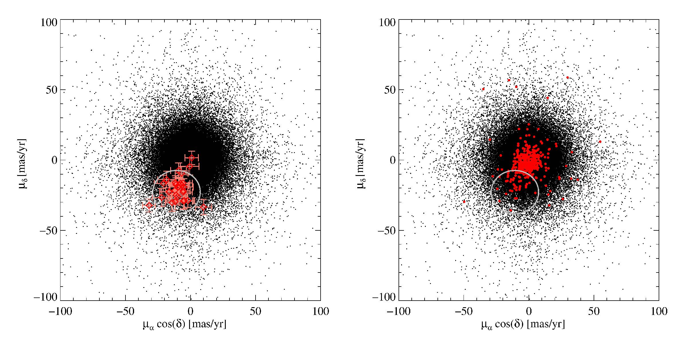
Figure 3: Proper motions of objects in the Lupus 3 field, based on 11-12 yr baseline between the WFI and NEWFIRM data (black dots). Left: The red symbols show the measured proper motions for the sources identified as members in López Martí et al. (2011). The ellipse depicts the $2\sigma$ criterion used for the proper motion candidate selection (see Section 3.2). Right: Red dots mark the proper motions of our 409 candidates selected from optical and NIR photometry. There are 59 candidates that pass both photometric and proper motion selection criteria.

3.2 Proper motions

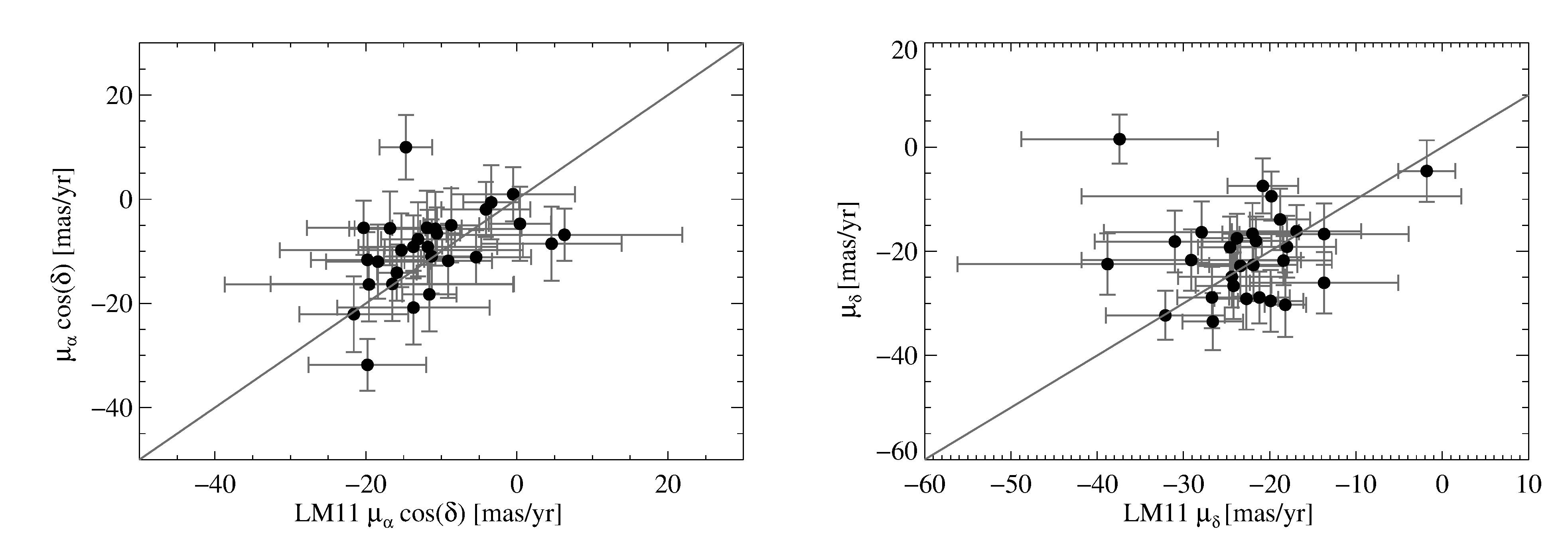
Figure 4: Comparison of the proper motions of the Lupus 3 members from López Martí et al. (2011) and this work. A line $x=y$ is shown as a solid line.

Proper motion measurements are based on the WFI dataset obtained between May 28th and June 3rd 1999 and our NEWFIRM data from June 2010 and May 2011. Whenever possible, we use the data from 2011, to assure the longest time baseline. In the following we describe in detail all the steps performed:
(1) The overlapping fields were first divided into sub-regions with the maximum size of $3^{\prime}\times 3^{\prime}$, and with an overlap of 0$\farcm$5 between the adjacent fields. We find that an area of this size typically contains a high number of sources that can be used for astrometric transformations, while being reasonably small to minimize the effects of field distortions.
(2) The absolute coordinate calibration shows systematic offsets of up to $12^{\prime\prime}$ between epochs in some regions, which poses a problem with cross-referencing individual sources, given the on-sky source density in Lupus 3. It is therefore crucial to apply an initial offset to the coordinates in one of the epochs, to assure the correct source registration in the two epochs. To determine the offset for each sub-region created in the first step, we create two images of the same size as the NEWFIRM and WFI sub-region of interest. The images have value of 1 at the positions equivalent to the centroid pixels of bright stars, and zero elsewhere. These images are then cross-correlated to obtain an average shift applied to a particular region;
(3) In this step we cross-match the catalogs based on right ascension and declination. This step is used only to identify individual sources in the two epochs, but not to calculate proper motions. The maximum matching radius of $2^{\prime\prime}$ was used, which is equivalent $\sim 170\,$mas yr^-1 over the 11-12 yr baseline.
(4) We apply a cutoff in magnitude for the matching sources, in order to discard saturated and faint ones (we keep all the sources with $J\approx 15.5-17.5$). The remaining sources are used in the next step to calculate a transformation of WFI positions to NEWFIRM coordinates. The number of sources used for the transformation in each sub-region varies between 80 and 400, with an average of 240;
(5) In the final step we calculate a polynomial that describes the transformation of the WFI detector ($x,y$) positions into the NEWFIRM coordinate frame for each sub-region, using the IDL procedure POLYWARP. In order to avoid the uncertainties in the absolute coordinate calibration, this step was performed in detector coordinates relative from one dataset to the other. We tested a 2nd and a 3rd degree polynomial and find that the two transformations give very similar final results, which is expected given the large number of sources available to calculate the transformation. Any polynomial with a degree $\geq 2$ corrects for shift and rotation between the fields, and also largely compensates for the distortions of the two detectors (e.g. Schödel et al. 2009). After applying the transformation, a proper motion was calculated for each source. Since the vast majority of stars used to calculate the transformation between the epochs are not Lupus members, we expect a circularly symmetric distribution around (0,0) in the proper motion space. We note that some of the members might have been included in the transformation, but their number compared to the total number of sources in our survey area is negligible, and thus does not influence the results. Finally, proper motions for the sources towards Lupus 3 are shown as black dots in Figure 3.

In order to assess the uncertainties of the proper motion measurements, we use the fact that the chips were divided into overlapping sub-regions in step (1) described above. This allows us to derive the uncertainties by comparing proper motions of common sources that were obtained using different sets of reference stars. For each NEWFIRM field, we adopt a common uncertainty calculated as a standard deviation of all the differences obtained from the overlapping regions in each field. For the sources with more than one measurement, the average is adopted as the final proper motion value.

López Martí et al. (2011) performed a kinematic study of the bright objects in the Lupus regions and found the average proper motion of the Lupus 3 members to be $v_{\alpha}=-10.7\pm 9.1\,$mas yr^-1, and $v_{\delta}=-22.8\pm 7.7\,$mas yr^-1. The uncertainties quoted here represent the standard deviation of the measurements for Lupus 3 given in Table 2 of López Martí et al. (2011). We select all the sources within an ellipse centered at (-10.7, -22.8) mas yr^-1 and with the semi-major axes equal to two times the above quoted uncertainties. This list was cross-matched with the photometric candidate catalogue described in the previous section, resulting finally in the list of 59 high-priority candidate members (“$IJ$-pm” sample; shown as filled black circles in Figure 2). The proper motions of the members in common with López Martí et al. (2011) are shown as red symbols in the left panel of Figure 3, on top of the circular proper motion distribution of all other sources in our field (black dots). The right panel shows the proper motions of the photometric candidates identified in this survey (red points).

Figure 4 shows a comparison between the proper motions of the Lupus 3 members from López Martí et al. (2011) and the proper motions of these same sources obtained in this work. There are in total 40 matching objects. While virtually all of these sources are saturated in WFI images, the brightest ones show severe saturation effects such as strong CCD leaking, which can seriously affect the astrometry. We therefore discard the extremely saturated sources with I${}_{C}>12.2$. The agreement between the two sets of proper motions is satisfactory, with all proper motions agreeing within $3\sigma$.

3.3 Mid-infrared selection

We retrieved the Spitzer IRAC and MIPS photometry of Lupus 3 from the Legacy Program data archive available at the Spitzer Science Center, using the “High reliability catalog” (HREL) created by the “Cores to Disk” (c2d) Legacy team, made available at the SSC Web site .

The $Spitzer$ catalogue was cross-correlated with our $i$-band catalogue, requiring the separation of $2^{\prime\prime}$ or better, and uncertainties $\leq 0.2\,$mag in the first four IRAC bands. To select the MIR-excess sources, we require $I3-I4\geq 0.4$ and $I1-I2>0$. This selection contains 75 sources, shown in Figure 5 as dots to the right of $I3-I4\geq 0.4$ line. Squares mark the 11 sources selected for follow-up spectroscopy. Of the 75 Spitzer-IRAC candidates, there are 19 sources that satisfy the proper motion criterion applied to the $iJ$ candidate list, and were included in the high-priority candidate list supplied to the VIMOS allocation software (we name this list the “IRAC-pm” sample). The Spitzer-IRAC list and the $iJ$ photometric candidate list have 7 objects in common.

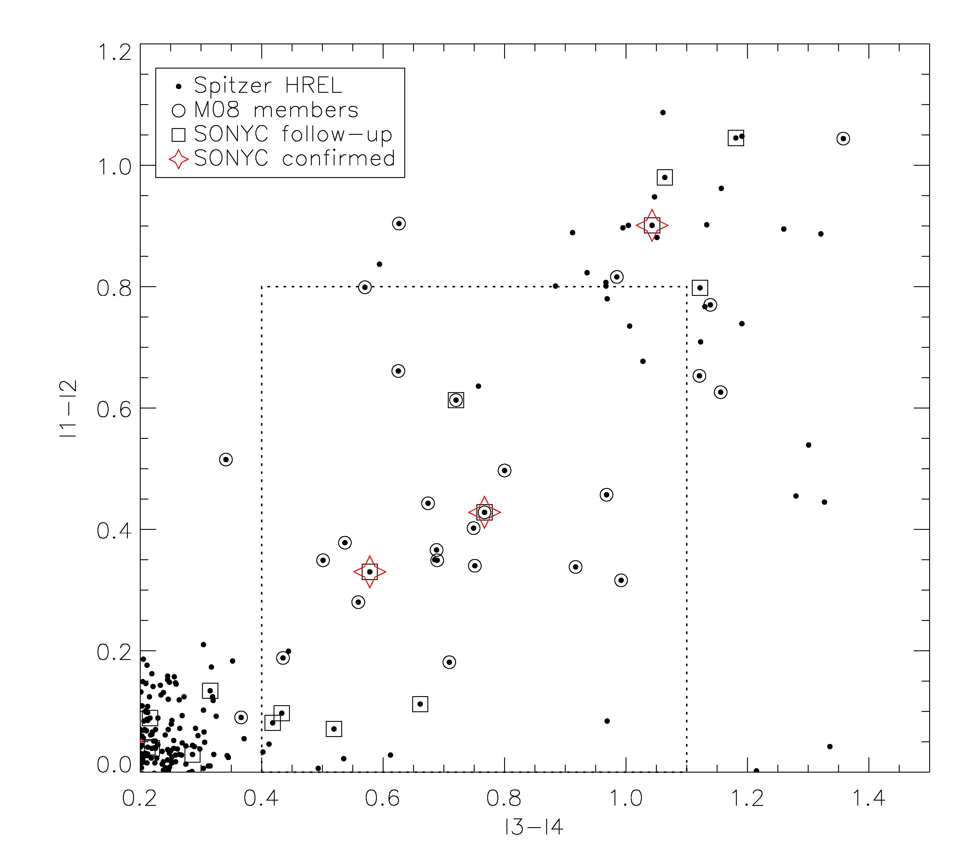
Figure 5: [3.6]-[4.5], [5.8]-[8.0] diagram constructed from $Spitzer$ IRAC photometry, for the objects matched with our optical catalog. The dashed line denotes the area where Class II objects are located, based on Allen et al. (2004). Open circles mark the collection of YSOs and pre-main sequence stars from Merín et al. (2008). Squares mark the objects whose spectra were obtained as part of the SONYC follow-up, and the red stars mark the three confirmed VLMOs.

4 Spectral analysis

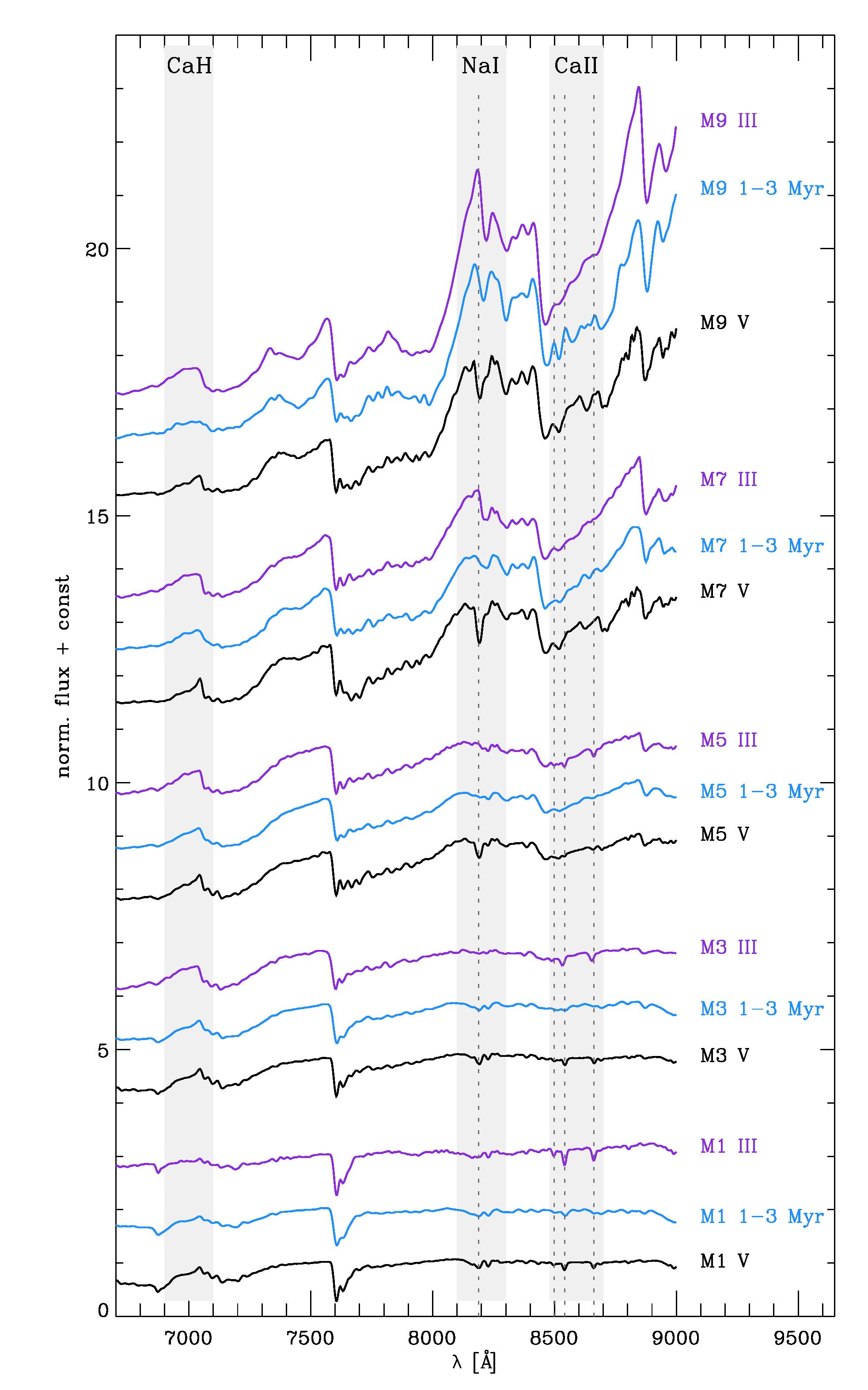
Figure 6: Part of the spectral sequence used for the spectral type fitting. Templates include dwarf and giant stars with spectral type M1 to M9, as well as the young members of star forming regions. Three gravity-sensitive spectral regions are shaded: (1) the 7000Å region affected by CaH absorption, (2) the region around Na I absorption feature at $\sim 8200\,$Å, and (3) the CaII absorption triplet at $\sim 8600\,$Å. The average wavelength of the Na I doublet, and the CaII triplet are marked by the vertical dashed lines. The spectra have been smoothed to match the spectral resolution of VIMOS, and normalized at 7500 Å.

Slits were allocated to 123 out of 409 objects, selected from the optical CMD, using the VIMOS Mask Preparation Software (VMMPS). VMMPS allows for only two priority classes. In P89 the high priority list included the two proper-motion selected samples, thus containing 59 candidates from the “$IJ$-pm” sample, and 19 candidates from the “IRAC-pm” sample, while the rest were the photometrically-selected candidates from $IJ$ and $Spitzer$-IRAC lists. In P87, prior to our proper motion analysis, the high priority candidates were those from the selection box, and the rest were randomly chosen objects within the FOV. In total, we obtained spectra of 123 objects from the selection box, and 44 outside of it. Of the 123 spectra from the $IJ$ selection box, 32 are from the “$IJ$-pm” sample. Diamonds in Figure  2 mark all the candidates with spectroscopy inside our selection box.

4.1 Preliminary selection

Our goal is to identify young, low mass stellar and substellar members of Lupus 3. Among the photometrically selected candidates, we may find contaminants such as embedded stellar members of Lupus 3 with higher masses, reddened background M-type stars, and (less likely) late M- and early L-type objects in the foreground. The red portion of M-dwarf optical spectra is dominated by molecular features (mainly TiO and VO; Kirkpatrick et al. 1991, 1995), which allows a relatively simple preliminary selection of candidates based on visual inspection. Here we included all the objects with clear evidence, but also, for the sake of caution, those objects with only tentative evidence of molecular features. Another property that was used in the selection is the slope, which should be positive in the red portion of the optical regime for M-type stars. Earlier stellar types typically have negative slopes, or appear flat (late K-type). Among the rejected spectra we mainly find flat spectra with no, or with very weak indication of molecular features (late K-dwarfs, or reddened earlier-type stars), and reddened featureless spectra (background or embedded stars of spectral type earlier than K). We also looked for the H_α emission at 6563 Å; only in one case an object was selected solely on the account of showing H_α, and despite the spectrum showing no prominent features characteristic for the M-type stars. After this preliminary selection, our sample contains 27 spectra. 26 of the selected spectra are photometric candidates, while 1 source appears bluer than expected for Lupus members. This source, SONYC-Lup3-6, will discussed in more detail in Section 4.8.

4.2 Spectral features as membership indicators

VIMOS was used in the spectroscopic part of the SONYC campaign in Cha-I (Mužić et al., 2011). The analysis presented here is partly similar to the one in that paper. Since the Cha-I observations in the first half of 2009, VIMOS was equipped with new, more red-sensitive detectors, which substantially decreased fringing that previously contaminated spectra longwards of 8000 Å. This is fortunate not only because our wavelength range is increased, but also because it allows us to analyze the gravity-sensitive Na I features at $\sim\,$8200 Å, which can provide an important constraint for the age of each observed object.

Youth provides strong evidence for cluster membership. We use the following features to identify members of Lupus 3:
(1) Na I doublet at 8183/8195  Å, which shows a change in equivalent widths, and a strong increase in the depth of absorption with increasing the surface gravity (e.g. Martín et al. 1999; Riddick et al. 2007; Schlieder et al. 2012). Although the individual lines of the doublet cannot be resolved in our spectra, the overall strength of the feature can still be used to assess the membership in the cluster even at low spectral resolutions.
(2) The spectral region $\sim 6900-7100$Å, shaped by TiO and CaH bands, also strongly affected by gravity at M types (Kirkpatrick et al., 1991). In particular, CaH absorption shortward of 7050 Å is stronger in M-type dwarfs, making the peak of the feature appear sharper in dwarfs, and rather blunt in giants.
(3) H_α emission, which is usually interpreted as a sign of accretion, and thus can be used as additional evidence for youth.
(4) The CaII triplet lines in absorption at 8498Å, 8542Å, and 8662Å  are prominent in late-K through mid-M giants, and are weaker in dwarfs (Kirkpatrick et al., 1991). This feature can help in identifying giant contaminants at early-M spectral types where Na I doublet becomes of limited use.

The points (1), (2) and (4) are demonstrated in Figure 6, showing a part of the spectral sequence (M1 to M9 with a step of 2 spectral subtypes) of giants, dwarfs, and members of young star forming regions (see Section 4.3 for detailed information on spectra and citations). The sodium absorption is much stronger in field dwarfs when compared to low-gravity atmospheres, and thus can be used to discard background field dwarfs with SpT later then M4 from our sample. Also, in the low-resolution spectra of dwarfs, the absorption feature is deepest at about the average wavelength of the Na I doublet (vertical line in Figure 6), and appears symmetric around it. On the other hand, the feature appears asymmetric in giants with the minimum slightly shifted towards longer wavelengths. This property can be used to distinguish between giants and low-gravity young objects at spectral types later than $\sim$M6. Determination of the spectral class is less straightforward at early spectral types (M2-M3), where the CaH feature at 7000Å and Ca II triplet can provide additional help. At M1 and earlier, the low-resolution spectra start to be of limited value for membership determination.

The equivalent width (EW) of H_α line in emission is often used to distinguish the accreting objects from the non-accretors. While the chromospheric H_α emission is expected to be found in most pre-main sequence M-dwarfs due to magnetic activity, larger equivalent widths observed in Class II objects are usually interpreted as a consequence of accretion and/or outflows (e.g. Scholz et al. 2007; Stelzer et al. 2013). White & Basri (2003) propose the EW(H_α) for actively accreting stars to be larger than 3Å for K0 – K5 stars, $>$10Å for K7 – M2.5, $>20$Å for M3 – M5.5, and $>40$Å for M6 – M7.5 stars. A similar criterion, but with finer division with respect to spectral type, and extended to the substellar regime, was derived by Barrado y Navascués & Martín (2003). The EW(H_α) for the SONYC objects in Lupus 3 are given in Table 4.4. SONYC-Lup3-1, 7, and 10 are revealed as strong accretors, and SONYC-Lup3-2, 8, and 11 are clearly non-accretors. The remaining objects with measured EW(H_α) all appear to be undergoing accretion according to the Barrado y Navascués & Martín (2003) criterion, whereas SONYC-Lup3-5, 6, and 12 fall slightly below the thresholds set by White & Basri (2003) for their respective spectral types.

4.3 Spectral classification

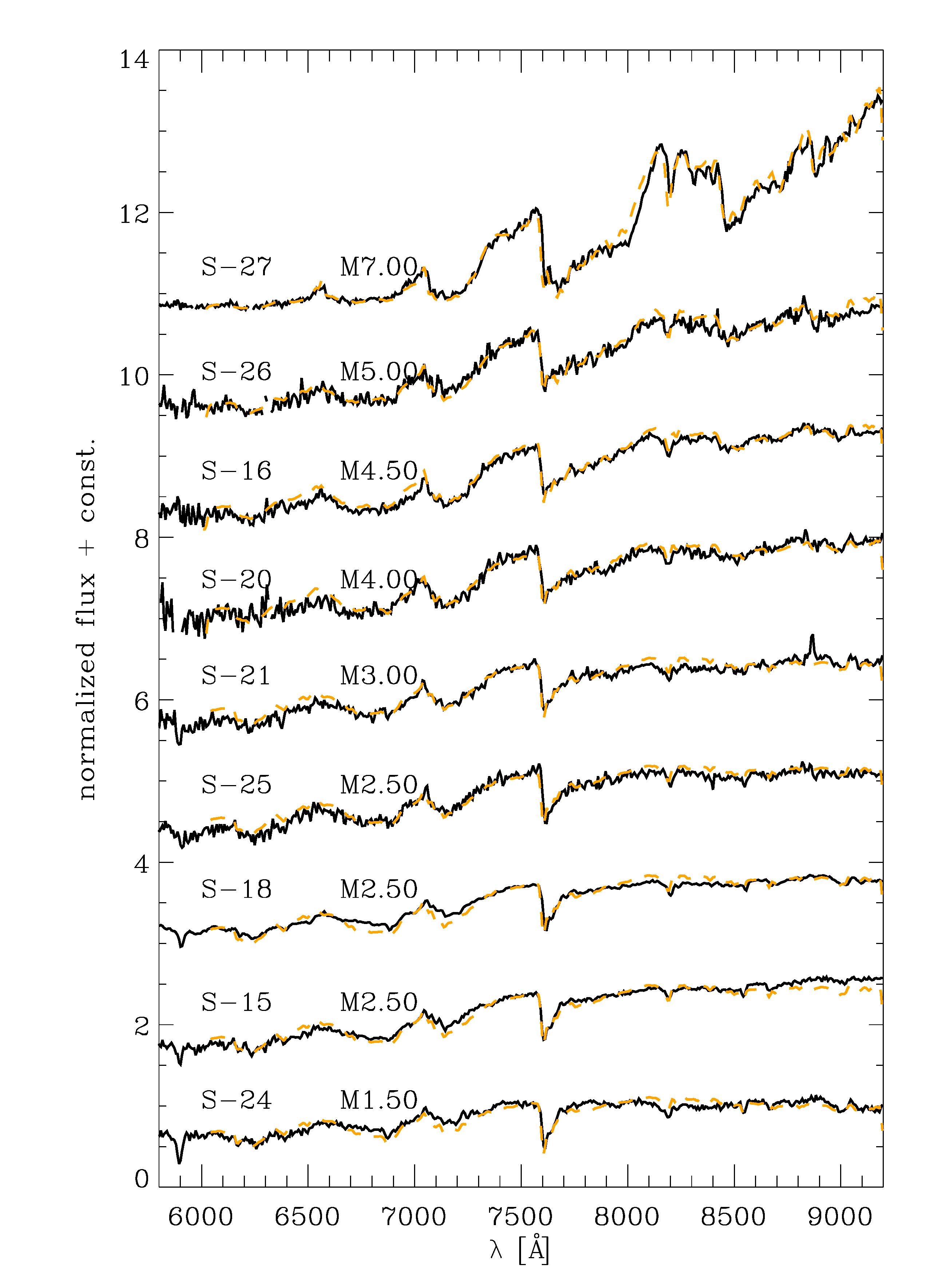
Figure 7: Spectra of the objects identified as field dwarfs (Table 4.4; black), along with the best-fit spectra (orange dashed line). The spectral resolution of the fit templates has been reduced in order to match the resolution of our spectra. Each spectrum has been corrected for extinction (see Table 4.4), but not for the atmospheric absorption.

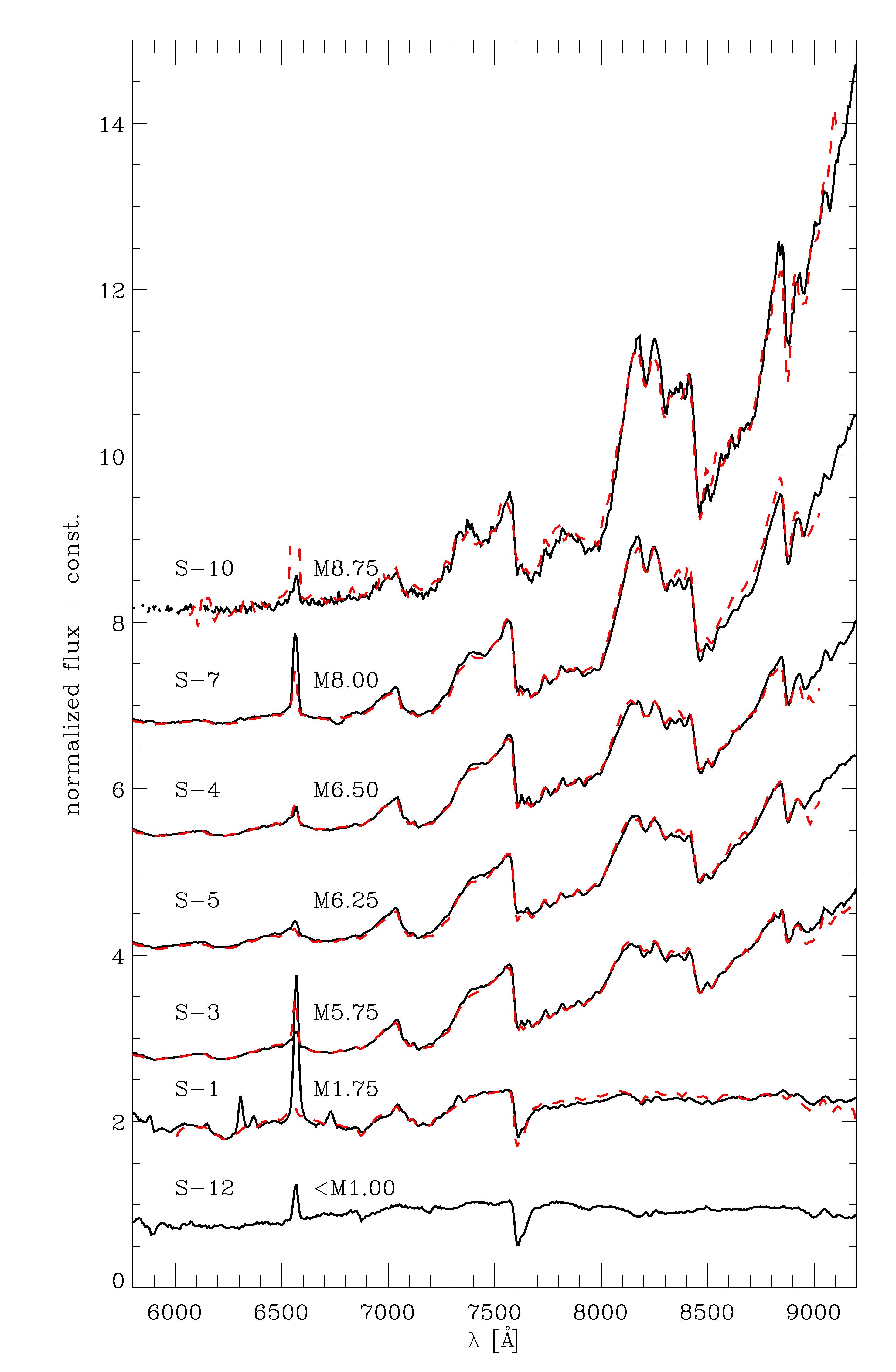
Figure 8: Spectra of the objects identified as probable members of Lupus 3 (Table 4.4; (black), along with the best-fit spectra of members of young star forming regions (red dashed line). The spectral resolution of the fit templates has been reduced in order to match the resolution of our spectra. Each spectrum has been corrected for extinction (see Table 4.4), but not for the atmospheric absorption.

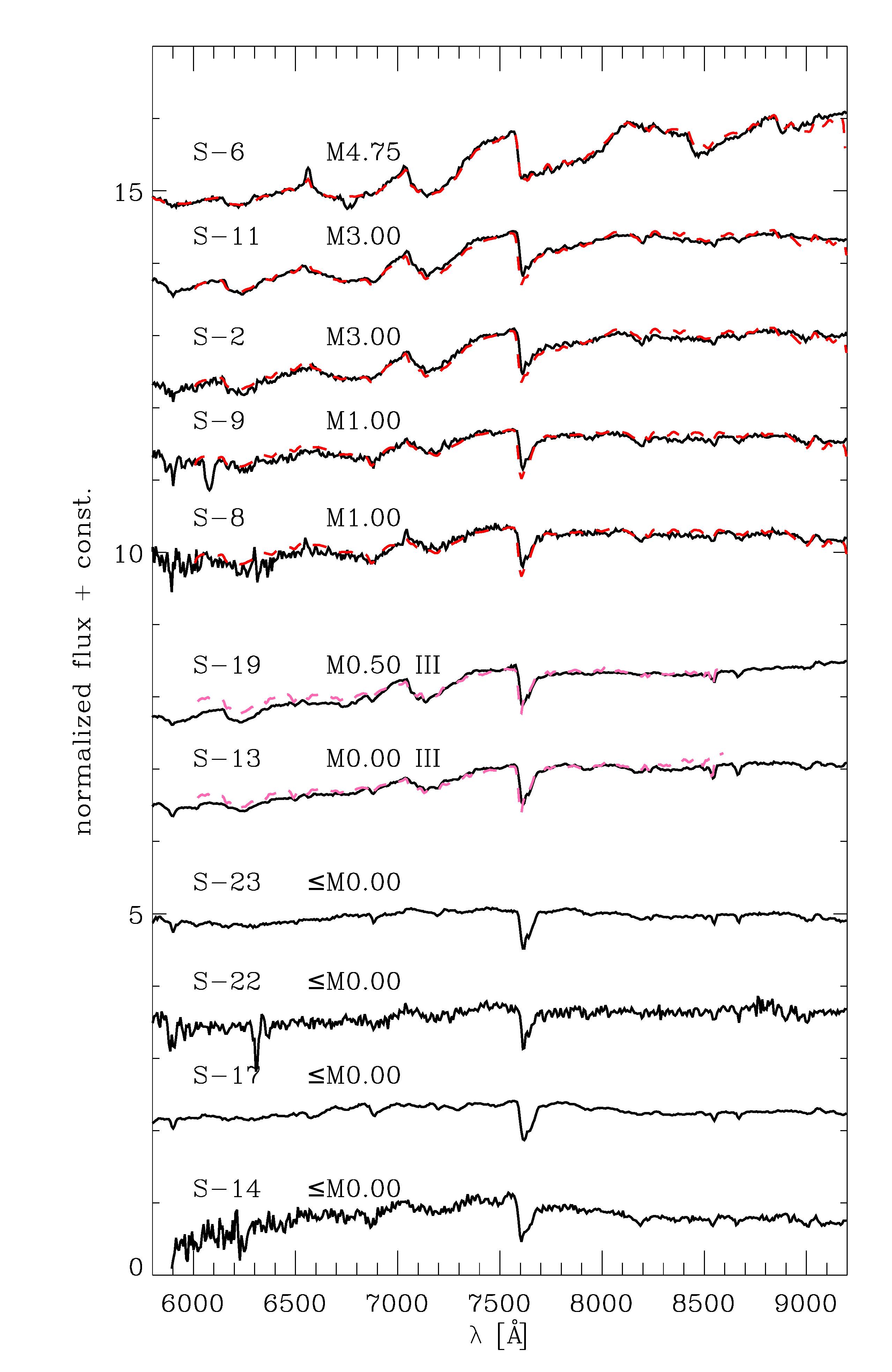
Figure 9: Spectra of the objects identified as giants, or with uncertain classification (Table 4.4; black), along with the best-fit spectra (dashed colored line). The spectral resolution of the fit templates has been reduced in order to match the resolution of our spectra. Each spectrum has been corrected for extinction (see Table 4.4), but not for the atmospheric absorption.

To determine spectral type and extinction of selected candidate members, we compare each spectrum to an empirical grid consisting of spectral templates of field dwarfs, giants, and members of young star forming regions with spectral types M1 to M9. A grid of field dwarfs separated by the 0.5 spectral subtype was created by averaging a number of available spectra at each sub-type. In case of giants, the grid consist of a collection of available spectra, with a step of 0.5 - 1 spectral subtypes . The grid of young objects (1-3 Myr) consists of the spectra of objects in Cha I, Taurus, and $\eta\,$Cha (Luhman et al., 2003a; Luhman, 2004a, b, c), with steps of 0.25-0.5 spectral subtypes.

Spectral type and extinction can be fitted simultaneously. The template spectra were first smoothed to match the resolution of the VIMOS spectra, and rebinned to the same wavelength grid. The region around the H_α line was masked. The best fit parameters were determined by minimizing the test value $\chi$ defined as

$$\chi=\frac{1}{N}\sum_{i=1}^{N}\frac{(O-T)^{2}}{T},$$ (1)

where O is the object spectrum, T the template spectrum, and N the number of data points.

As mentioned before, spectral classification becomes less reliable at low resolution for objects of spectral type M3 and earlier. It is therefore not surprising that at these early spectral types, the fitting scheme gives similar results for different spectral classes. Some level of degeneracy with respect to spectral classes is also present at later spectral types, but only in a few cases. It is therefore clear that the final assessment of class (i.e. membership) cannot be based on this fitting scheme only. However, there is much less degeneracy present with respect to the spectral subtype and A_V, also for the objects with degenerate spectral class. Typically, several best-fit results cluster within $\pm 1$ spectral subtype and $\pm 1\,$mag in A_V, or less, from the best-fit value. We therefore adopt these values as typical uncertainties of the fitting procedure.

To determine membership status of an object, several best fits at each spectral class are inspected visually, in order to check for the presence or shape of the spectral features discussed in the previous section.

Of the initial 27 spectra we started with, 9 objects are classified as field dwarfs because of the deep Na I absorption and the lack of H_α emission (see Figure 7). Two spectra are best represented by spectra of early-M giants, while four objects have M-dwarf features that are less pronounced than in M1 dwarfs, i.e. are probably of earlier spectral type (bottom 6 spectra in Figure 9). The spectra of the latter 4 objects (SONYC-Lup3-14, 17, 22, and 23) all show evidence for CaII triplet in absorption. The spectra of SONYC-Lup3-17 and 23 also have very weak or non-existent Na I absorption, thus are probably background giants. The spectra of SONYC-Lup3-14 and 22 have lower S/N, which poses a difficulty in final classification. The depth of the Na I in the spectrum of SONYC-Lup3-14 hints to a high-gravity atmosphere, but for the sake of caution, we prefer to keep the membership status of both objects as uncertain.

Seven spectra are best fit by young dwarf templates with no degeneracy in spectral class (SONYC-Lup3-1, 3, 4, 5, 6, 7, and 10). The spectrum of the object SONYC-Lup3-10 is best matched with a M8.75 young dwarf template, that was derived by averaging the spectra of Taurus members KPNO09 (M8.5) and KPNO12 (M9) from Luhman (2004c). All of these 7 objects also show H_α emission, and appear to have weak Na I absorption, suggesting some kind of low-gravity atmosphere. All 7 objects are also proper motion candidates. SONYC-Lup3-12 exhibits strong H_α emission, but its spectrum is outside our fitting grid (earlier than M1). The shape of the Na I feature reveals a low-gravity atmosphere, while the lack of the Ca II triplet in absorption make it less probable to be a giant. Furthermore, its proper motion argues in favor of its membership in Lupus, and therefore we include SONYC-Lup3-12 in the list of candidate members. The spectra of these 8 best candidates for membership in Lupus are shown in Figure 8, with exception of SONYC-Lup3-6 which is, for the reasons that will become apparent in the next sections, classified as uncertain and shown in Figure 9.

The nature of the remaining 4 objects of early M spectral type (SONYC-Lup3-2, 8, 9 and 11) remains uncertain at this stage. In Figure 9 we show their spectra together with the best-fit young dwarf templates, but we note that other classes might give equally satisfactory fit. The CaH and Na I regions for all 4 objects fit better in the dwarf class, rather than giants. The CaII triplet absorption is present, which indicates that none of these objects is young.

4.4 Model fitting

In order to derive effective temperatures for the SONYC objects, we perform the spectral model fitting using the BT-Settl (Allard et al., 2011) and AMES-Dusty (Allard et al., 2001) models. Model spectra are smoothed by a boxcar function beforehand, to match the wavelength step of the VIMOS spectra. The three main parameters that affect the spectral shape are the effective temperature ($T_{\mathrm{eff}}$), gravity (log$\,g\,$), and interstellar extinction ($A_{V}$). Fitting the models to our low-resolution spectra does not allow an unambiguous determination of all the three parameters at the same time. We therefore keep log$\,g\,$ constant for each object, and assume the value of 3.5 (or 4 in case of AMES-Dusty models above 3000 K) for the objects identified as probable young dwarfs, 5 for the field dwarfs, and 3 for the giants (in this case only BT-Settl models are used). For all the spectra classified as uncertain, we use the intermediate value of log$\,g\,$, i.e. the same as for young dwarfs. The fitting procedure of $T_{\mathrm{eff}}$ and $A_{V}$ is identical to the one described in Mužić et al. (2011). $T_{\mathrm{eff}}$ is varied between 2000 K and 4500 K in steps of 100 K, and $A_{V}$ from 0 to 10, in steps of 0.5 mag. To de-redden our spectra, we apply the extinction law from Cardelli et al. (1989), assuming $R_{V}\,$= 4.

The spectra of objects in Table 4.4 with the best-fit atmosphere models are shown in the appendix (Figures 14 and 15), and the results of our spectral fitting procedure for these objects are given in Table 3. The uncertainty is 100 K for the derived effective temperature, and 0.5 mag for the extinction, which reflects the spacing of the grid.

Table 2: Photometry and spectral types for the objects of spectral type M, or slightly earlier, identified towards Lupus 3.

ID	$\alpha$(J2000)	$\delta$(J2000)	$i$	$J$	$K$	A${}_{V}^{phot}$	SpT	A${}_{V}^{SpT}$	$\mu_{\alpha}cos\delta$	$\mu_{\delta}$	$\mu-$	EW(H$\alpha$)	membership	comments
			(mag)	(mag)	(mag)	(mag)		(mag)	(mas yr-1)	(mas yr-1)	cand?	(Å)
S-1	16:07:08.55	-39:14:07.8	17.3	14.6	11.5	11.5	M 1.75	3.0	-4.2$\pm$5.2	-21.2$\pm$4.7	y	-77.6	Lupus 3	M08
S-2	16:07:33.82	-39:03:26.5	19.4	16.2	14.1	6.0	M 3.00	5.0	0.4$\pm$7.1	-16.3$\pm$5.9	y	-4.9	uncertain
S-3	16:07:55.18	-39:06:04.0	16.2	13.5	11.4	5.9	M 5.75	2.0	-12.4$\pm$7.1	-22.8 $\pm$5.9	y	-37.2	Lupus 3	M6.5, C09, G06
S-4	16:08:04.76	-39:04:49.6	17.0	13.9	12.4	2.9	M 6.50	1.0	-8.1$\pm$7.1	-22.6 $\pm$5.9	y	-44.4	Lupus 3	M7, C09
S-5	16:08:16.03	-39:03:04.5	15.5	12.5	11.1	2.5	M 6.25	1.0	-9.3$\pm$7.1	-19.9 $\pm$5.9	y	-37.5	Lupus 3	Par-Lup3-1; M7.5, M5.5
S-6	16:08:59.52	-38:56:20.8	19.1	17.4	16.7	0.0	M 4.75	0.0	-6.5$\pm$7.1	-19.4$\pm$5.9	y	-18.6	uncertain
S-7	16:08:59.53	-38:56:27.8	17.1	13.9	12.7	1.3	M 8.00	0.5	-8.8$\pm$7.1	-19.6 $\pm$5.9	y	-185.7	Lupus 3	M8, G06
S-8	16:10:18.13	-39:10:33.6	19.8	16.2	13.8	7.3	M 1.00	6.5	-16.2$\pm$5.3	-9.8$\pm$5.0	y	-4.6	uncertain
S-9	16:11:26.34	-39:02:17.1	19.3	16.2	14.0	6.4	M 1.00	5.5	-14.6$\pm$5.3	-11.3 $\pm$5.0	y	$\cdots$	uncertain
S-10	16:09:13.43	-38:58:04.9	19.5	16.1	14.9	1.5	M 8.75	0.0	-13.8$\pm$7.1	-20.9 $\pm$5.9	y	-48.8	Lupus 3
S-11	16:12:05.91	-39:04:07.5	18.7	15.7	14.4	1.5	M 3.00	3.0	-24.7$\pm$5.3	-20.5 $\pm$5.0	y	-5.4	uncertain
S-12	16:11:18.47	-39:02:58.2	18.0	15.1	13.3	4.2	$<$M 1	$\cdots$	-6.1$\pm$5.3	-8.5 $\pm$5.0	y	-12.1	Lupus 3
S-13	16:07:36.48	-39:04:53.8	15.7	12.9	10.6	7.1	M 0.00	3.5	-3.4$\pm$7.1	1.1$\pm$5.9	n	$\cdots$	III
S-14	16:08:01.42	-39:10:16.1	19.9	16.4	14.0	7.7	$<$M 1	$\cdots$	-8.4$\pm$7.1	-12.7$\pm$5.9	y	$\cdots$	uncertain
S-15	16:07:52.46	-39:09:48.1	19.0	15.6	13.2	7.6	M 2.50	4.7	-29.8$\pm$7.1	-23.1 $\pm$5.9	y	$\cdots$	V
S-16	16:10:14.95	-39:10:16.2	19.9	16.4	14.3	5.7	M 4.50	4.7	5.9$\pm$5.3	24.0 $\pm$5.0	n	$\cdots$	V
S-17	16:11:56.11	-39:08:23.8	15.3	12.8	11.1	4.2	$<$M 1	$\cdots$	-0.3$\pm$5.3	11.1 $\pm$5.0	n	$\cdots$	III
S-18	16:11:09.03	-39:06:22.7	16.8	14.3	12.5	4.5	M 2.50	3.0	-11.4$\pm$5.3	-21.7 $\pm$5.0	y	$\cdots$	V
S-19	16:11:39.24	-39:06:32.8	15.4	12.5	10.4	6.0	M 0.50	3.0	-5.7$\pm$5.3	-5.4 $\pm$5.0	y	$\cdots$	III
S-20	16:11:36.20	-39:02:36.9	20.4	16.8	14.6	6.9	M 4.00	5.3	3.9$\pm$5.3	17.1 $\pm$5.0	n	$\cdots$	V
S-21	16:11:33.34	-38:59:44.3	19.9	16.5	14.3	4.9	M 3.00	4.5	7.8 $\pm$5.3	1.1 $\pm$5.0	n	$\cdots$	V
S-22	16:10:47.49	-38:57:12.4	20.4	17.1	16.2	0.0	$<$M 1	$\cdots$	$\cdots$	$\cdots$	$\cdots$	$\cdots$	uncertain
S-23	16:10:45.40	-38:54:54.9	16.1	14.3	12.9	2.1	$<$M 1	$\cdots$	-7.9$\pm$5.3	-1.9 $\pm$5.0	n	$\cdots$	III	M08, C09
S-24	16:07:09.06	-39:01:07.6	19.8	18.1	16.6	2.8	M 1.50	1.5	7.4$\pm$5.2	3.6$\pm$4.7	n	$\cdots$	V
S-25	16:12:04.96	-39:06:11.4	19.9	17.9	16.0	5.1	M 2.50	3.0	1.0 $\pm$5.3	2.7 $\pm$5.0	n	$\cdots$	V
S-26	16:10:56.40	-39:04:31.7	19.1	17.3	15.7	3.4	M 5.0	2.5	35.4$\pm$5.3	0.9 $\pm$5.0	n	$\cdots$	V
S-27	16:11:15.08	-39:07:15.0	18.1	16.4	14.7	3.6	M 7.0	0.0	$\cdots$	$\cdots$	$\cdots$	$\cdots$	V

References. — (a) Comerón et al. (2003); (b) Mortier et al. (2011); (c) Allen et al. (2007); (d) Comerón et al. (2013)

Table 3: Effective temperature and extinction derived from models, for the objects of spectral type M (or slightly earlier) towards Lupus 3.

ID	$T_{\mathrm{eff}}^{A-D}$	A${}_{V}^{A-D}$	$T_{\mathrm{eff}}^{BT-S}$	A${}_{V}^{BT-S}$	$T_{\mathrm{eff}}^{C}$	A${}_{V}^{C}$
	(K)	(mag)	(K)	(mag)
S-1	3900	3.0	3800	3.0	4400	7.1
S-2	3600	6.0	3500	5.0	$\cdots$	$\cdots$
S-3	3100	4.0	3000	3.0	2950	2.3
S-4	3000	4.0	3000	3.5	2900	3.5
S-5	3000	3.5	2900	2.0	2800	2.0
S-6	3100	0.5	3200	0.0	$\cdots$	$\cdots$
S-7	2900	4.5	2800	3.0	2600	1.5
S-8	3900	6.5	3800	6.5	$\cdots$	$\cdots$
S-9	3900	5.5	3800	5.5	$\cdots$	$\cdots$
S-10	2600	4.0	2700	4.0	$\cdots$	$\cdots$
S-11	3700	4.0	3500	3.5	$\cdots$	$\cdots$
S-12	$>$3900	$\cdots$	4200	4.5	$\cdots$	$\cdots$
S-13	$\cdots$	$\cdots$	3900	4.5	$\cdots$	$\cdots$
S-14	3900	6.0	3800	6.5	$\cdots$	$\cdots$
S-15	3700	6.5	3600	6.0	$\cdots$	$\cdots$
S-16	3100	5.5	3000	4.0	$\cdots$	$\cdots$
S-17	$\cdots$	$\cdots$	4400	5.0	$\cdots$	$\cdots$
S-18	3800	4.5	3600	3.5	$\cdots$	$\cdots$
S-19	$\cdots$	$\cdots$	3900	4.0	$\cdots$	$\cdots$
S-20	3400	6.5	3200	5.5	$\cdots$	$\cdots$
S-21	3400	5.0	3300	4.5	$\cdots$	$\cdots$
S-22	$>$4000	$\cdots$	4100	2.5	$\cdots$	$\cdots$
S-23	$\cdots$	$\cdots$	4200	2.5	4400	2.7
S-24	3900	2.0	3800	2.0	$\cdots$	$\cdots$
S-25	3400	3.5	3300	3.0	$\cdots$	$\cdots$
S-26	3100	4.0	3000	2.5	$\cdots$	$\cdots$
S-27	2700	2.5	2800	1.5	$\cdots$	$\cdots$

Note. — A-D - AMES-Dusty (Allard et al., 2001);BT-S - BT-Settl (Allard et al., 2011); C - parameters derived by Comerón et al. (2009, a) and Comerón et al. (2013, b).

4.5 MIR excess

From the list of potential members selected from the IRAC data, we obtained spectra of 11 objects. Three of them are confirmed as VLM members of Lupus 3 (SONYC-Lup3-1, SONYC-Lup3-7 and SONYC-Lup3-10). Of the confirmed objects, all were originally selected from the $iJ$ selection. SONYC-Lup3-1 satisfies the YSO criteria from Merín et al. (2008). The fact that these three candidates exhibit disk excess further strengthens their membership in Lupus 3.

There is only one object in the $Spitzer$ photometric candidate selection (Figure 5) that appears as candidate YSO in Merín et al. (2008), but it was not confirmed in our work. Judged from the spectrum, this object (c2d source number 120; $\alpha=$16:10:45.40, $\delta=$-38:54:54.9) probably belongs to the spectral type K, i.e. it is too early for our spectral typing scheme to work. Therefore, while this object does not fall into the class of VLMOs that are the subject of this paper, we do not rule it out as a potential member. The remaining spectra also look earlier than M1, and do not show any evidence of H_α emission, and are therefore eliminated in our search for very-low-mass objects.

4.6 Hertzsprung-Russell Diagram

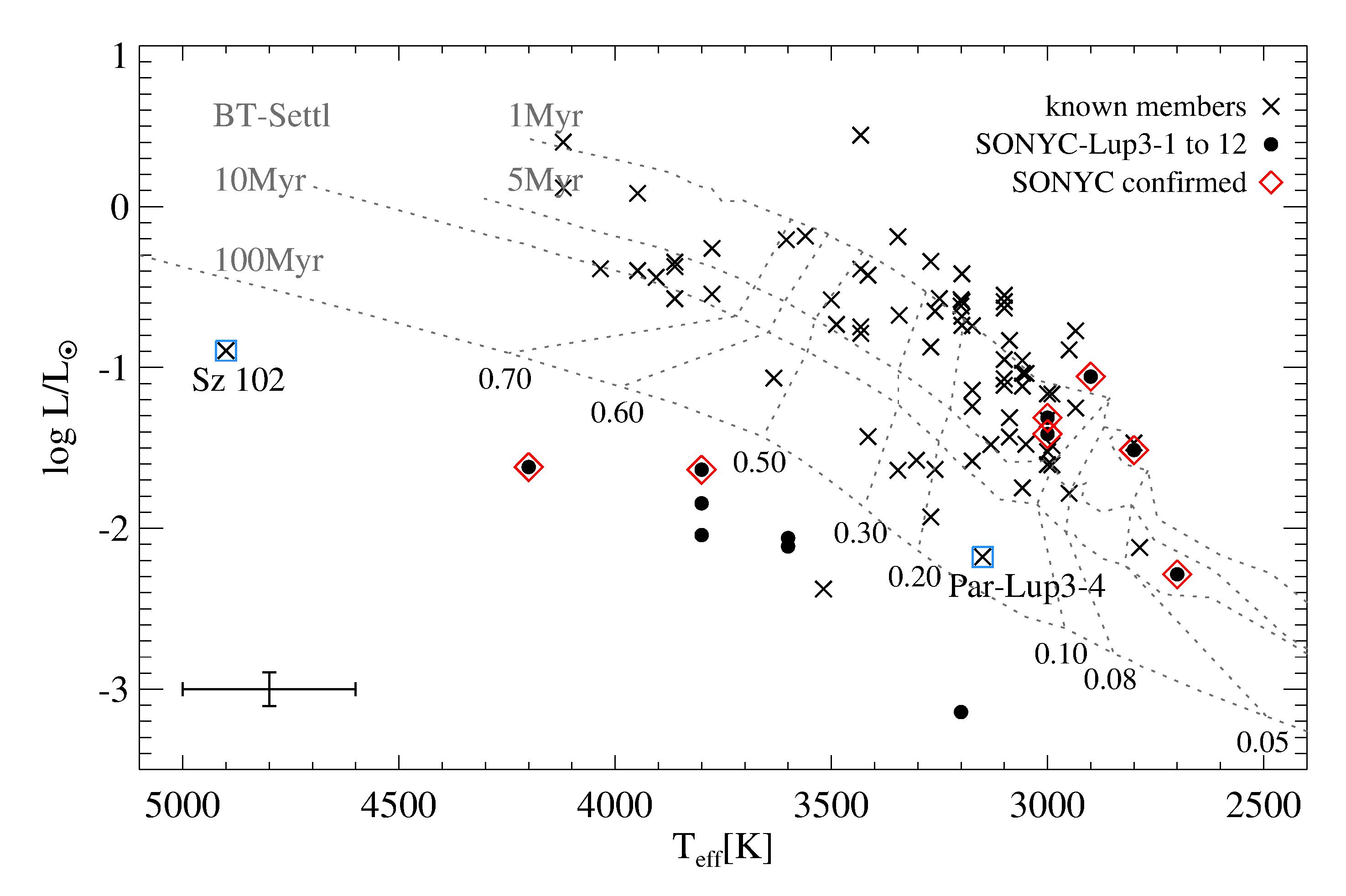
Figure 10: H-R diagram for the Lupus 3 members with existing $T_{\mathrm{eff}}$ or spectral type from the literature (crosses). Filled circles mark the sources SONYC-Lup3-1 to -12. Red diamonds mark the final subset of confirmed members of Lupus 3. The two well known examples of underluminous, emission line YSOs are labeled and marked with blue squares. The dashed lines show BT-Settl theoretical tracks for several ages spanning 1 and 100 Myrs.

In Figure 10 we show the Hertzsprung-Russell diagram, for the list of spectroscopically confirmed members shown in Table Substellar Objects in Nearby Young Clusters (SONYC) VIII: Substellar population in Lupus 3. The extinction was calculated by assuming the intrinsic color $(J-K)_{0}=1$, and extinction law from Cardelli et al. (1989) with R${}_{V}=4$. The adopted distance is 200 pc. Where available, we use $T_{\mathrm{eff}}$ estimates available from the literature. For the spectroscopically confirmed members that lack the $T_{\mathrm{eff}}$ information, we convert their spectral types to $T_{\mathrm{eff}}$ using the transformation established in Section 5.1.We calculate the bolometric correction in the $J-$band (BC_J) from the polynomial relation between BC_J and $T_{\mathrm{eff}}$ derived by Pecaut & Mamajek (2013) for pre-main sequence stars with ages of 5-30 Myr. The typical error-bar is shown in the lower left corner. The uncertainty in the $T_{\mathrm{eff}}$ is set to 200 K ($\sim$200 K for sources from Comerón et al. 2009, $\sim 300\,$K for Mortier et al. 2011, and $\sim 100\,$K for the rest). The error in luminosity takes into account the typical error in the observed $J$ magnitude (0.1 mag), distance ($\pm 20$pc), A_V ($\pm 1$ mag), and BC_J. We also show the BT-Settl isochrones for ages between 1 Myr and 100 Myr. Filled circles mark the 8 objects that were identified as possible members in Section 4.3, together with the 4 objects with uncertain membership status (SONYC-Lup3-1 through 12). We use $T_{\mathrm{eff}}$ and A_V as derived by comparison with the BT-Settl models.

The position of sources in H-R diagram can provide additional information about their nature. We can compare the positions of our sources in the H-R diagram, with the positions of the known members of Lupus 3. The large fraction of previously confirmed members is located between the 1 and 10 Myr isochrones, with a few also found below the 10 Myr isochrone. Among the latter are the two well known cluster members showing significant underluminosity for their spectral types, Sz 102, and Par-Lup3-4 (Krautter, 1986; Comerón et al., 2003) .

The H-R diagram positions of the five SONYC sources with estimated $T_{\mathrm{eff}}\leq\,$3000 K agree well with the positions of other Lupus members. These sources, SONYC-Lup3-3, 4, 5, 7, and 10, are therefore classified as members of Lupus 3. The remaining sources appear well below the 100 Myr BT-Settl isochrone. We compared our photometry with that from 2MASS, to check for variability as a possible cause of the underluminosity for some of these 7 sources. While SONYC-Lup3-6 is too faint to be detected by 2MASS, all the rest have photometry of a good quality in at least one of the J- and K-bands. SONYC-Lup3-1 shows a difference of 0.7 mag in J, and 0.1 mag in K-band; SONYC-Lup3-12 show a difference of 0.3 mag in the K-band (only an upper limit in J in 2MASS). The remaining sources show no evidence for variability, with differences between the two photometric datasets below 0.1 mag, i.e. comparable to the measurement errors. As mentioned in Section 4.3, SONYC-Lup3-2, 8, 9 and 11 were suspected to be non-members, and Figure 10 confirms it. The remaining three sources (SONYC-Lup3-1, 6 and 12) deserve special attention and will be discussed below. Finally, the lack of the objects with similar spectral types (early-to-mid M) having luminosities that would suggest membership in Lupus is easily explained by the saturation limit of the $i$-band catalog used for the selection

4.7 SONYC-Lup3-1

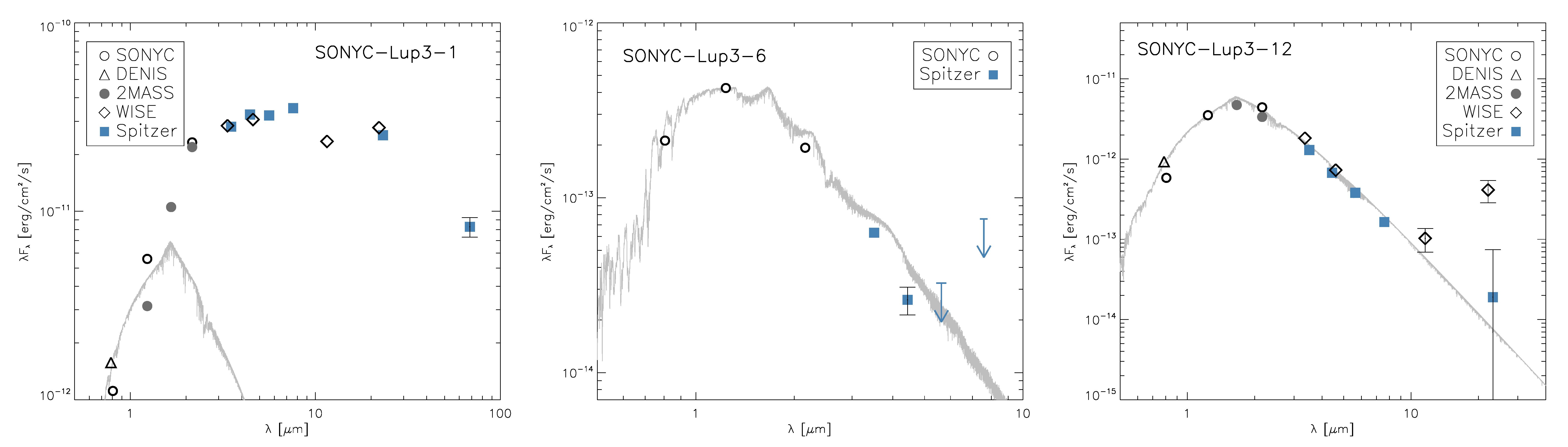
Figure 11: Spectral energy distribution of SONYC-Lup3-1, 6, and 12. Photometry comes from this work (open circles), DENIS (triangles), 2MASS (filled grey circles), $Spitzer$ IRAC and MIPS (squares), and WISE (diamonds). The uncertainties are comparable to or smaller than the size of the symbols, except for the points with the error bars shown.

In addition to being one of the strongest H_α emitters among our selected sources (EW(H_α)=-77.6Å), the spectrum of SONYC-Lup3-1 shows presence of forbidden lines, similar to those previously observed in spectra of Lupus 3 members Par-Lup3-4, Sz102, and Sz106 (Comerón et al., 2003). We identify the [OI] lines at 6300Å and 6364Å, [SII] line at 6731Å (possibly blended with [SII] line at 6716Å), and [OII] at 7329Å. Forbidden lines such as those identified here are commonly observed in actively accreting young stars, and their ratios can be used to estimate physical conditions in the circumstellar medium and mass-loss rates (Osterbrock, 1989). However, as discussed in Comerón et al. (2003), forbidden lines in T-Tauri spectra are usually split into separate components sampling different physical conditions, which cannot be distinguished with our low-resolution spectra. Moreover, our spectra do not allow definitive identification of some lines (e.g. [SII] at 6731 and 6716 Å). We therefore refrain from physical interpretation of the conditions causing this emission, and leave this to future studies at higher spectral resolution.

Two sources in Lupus 3 are reported in the literature to exhibit similar properties. Sz 102 appears underluminous for its spectral type, which was was first noted by Hughes et al. (1994). Krautter (1986) found Sz 102 to be associated with a bipolar jet and a Herbig-Haro object. This geometry suggests that we might be viewing the star through a nearly edge-on disk (Krautter, 1986; Hughes et al., 1994). Comerón et al. (2003) report the underluminosity of Par-Lup3-4, and a jet associated with Par-Lup3-4 was discovered in [SII] images by Fernández & Comerón (2005). Comerón et al. (2003) discuss three possible interpretations for the underluminosity and emission line spectra of the two objects:
(a) An edge-on disk blocking a part of the stellar light, (b) embedded Class I sources where the star is seen via the light scattered by the walls of cavities in the envelope, and (c) accretion-modified evolution, similar to what is described in Hartmann (1998) and Baraffe et al. (2009). High-resolution spectra of Par-Lup3-4 (Fernández & Comerón, 2005) reveal a double-peaked [SII] profile, implying that the low excitation jet is seen at a small angle with respect to the plane of the sky. The authors argue that at this inclination, only a flared disk could hide a star. Huélamo et al. (2010) studied the target SED from the optical to the sub-millimeter regime, and compared it to a grid of radiative transfer models of circumstellar disks. They find that Par-Lup3-4 is a Class II source, with an edge-on disk that naturally explains its underluminosity.

In Figure 11 we show the SED of SONYC-Lup3-1 in the range 0.8 - 70 $\mu$m. Open circles mark the optical and NIR photometry from the SONYC campaign, the filled grey circles show the 2MASS NIR photometry, squares $Spitzer$ MIR data, and diamonds the MIR photometry from WISE. The double-peaked shape of the SED with a dip around 10 $\mu$m is characteristic for an edge-on disk, where the NIR peak arises from the scattered light of the star obscured by a disk, and the emission at longer wavelengths comes from the dust (e.g. Wood et al., 2002; Pontoppidan et al., 2007; Huélamo et al., 2010). The radiative transfer SED modeling could shed more light on the properties of the putative disk around SONYC-Lup3-1, but since this is out of the scope of this paper, we refrain from discussing this source further. To calculate the luminosity of SONYC-Lup3-1 in Fig 10, we used the A_V=3.0 mag derived from fitting a model to the spectrum. The extinction calculated from the $J-K$ color is, however, significantly higher (A${}_{V}=11.5$ mag), and shifts the point in the H-R diagram in the y-direction such that it falls roughly onto the 10 Myr isochrone. We conclude that SONYC-Lup3-1 is probably a member of Lupus 3, with properties similar to Par-Lup3-4 and Sz 102. The MIR excess and the double-peaked SED suggest a presence of an edge-on circumstellar disk.

4.8 SONYC-Lup3-6

We obtained the spectrum of SONYC-Lup3-6 by chance alignment of the slit that was placed on SONYC-Lup3-7, which belongs to our high-priority candidate list. SONYC-Lup3-6 is located $\sim 7^{\prime\prime}$ north of SONYC-Lup3-7. With the $i-J$ color of 1.8, SONYC-Lup3-6 is too blue to be in our photometric candidate list, i.e. the colors suggest that the object is not a pre-main sequence source. In the HR diagram, it falls well below the 100 Myr isochrone. However, the spectral fitting procedure identifies the object as a young star of the spectral type M4.75. It shows low-gravity Na I signatures, H_α emission, and no evidence for Ca II triplet absorption. Furthermore, its proper motion satisfies the proper-motion membership criterion. From the EW(H_α) it is not clear whether SONYC-Lup3-6 undergoes accretion or not, as it falls close to the line that separates accretors from non-accretors (yes according to the criterion by Barrado y Navascués & Martín 2003, and no according to White & Basri 2003). If indeed a member of Lupus 3, SONYC-Lup3-6 might be a primary of a very wide binary system containing the M8 brown dwarf SONYC-Lup3-7. The projected separation of this hypothetical system would be $\sim$1400 AU. It would be, however, very difficult to explain a M4.75 primary that is several magnitudes fainter than its supposed secondary. We therefore classify the membership of SONYC-Lup3-6 as uncertain.

4.9 SONYC-Lup3-12

This object’s spectrum suggests a type earlier than M1, but was nevertheless selected in our preliminary analysis based on the obvious H_α emission observed in its spectrum (Figure 8). According to West et al. (2008), early M-dwarfs have shorter activity lifetimes when compared to the later M-dwarfs, which speaks in favor of SONYC-Lup3-12 being indeed young. However, as in the case of SONYC-Lup3-6, the EW(H_α) falls right at the border separating accreting objects from non-accretors (accretor according to the criterion by Barrado y Navascués & Martín 2003, and non-accretor according to White & Basri 2003). When compared to the spectra of other objects in our sample with similar early spectral type (e.g. SONYC-Lup3-17, 22, 23), we notice the lack of the CaII absorption lines, i.e. this object is likely not to be a giant. Based on this evidence, we tentatively include SONYC-Lup3-12 in the final list of the confirmed members. It shows no MIR excess, and therefore the edge-on disk morphology does not seem to be a plausible explanation for its underluminosity.

4.10 Summary of the results

From the candidate list containing 409 objects in the direction of Lupus 3 cloud, 123 objects were selected for the spectroscopic follow-up. 27 showed spectral features consistent with spectral type M, or slightly earlier. Fitting the spectra to an empirical grid of spectra of young dwarfs, field dwarfs and giants, combined with the proper motion assessment of membership, and the positions of the candidates in the HR diagram, we identify 9 field dwarfs, 4 background giants, and 7 probable members of Lupus 3, among which two show significant underluminosity for their spectral type. The nature of 7 sources remains uncertain. In Table 4.4 we list the 27 analyzed sources, and give their coordinates, photometry, spectral types, proper motions, EW(H_α), membership status, and references for those identified in the literature.

5 Results and discussion

In this section we use the members of Lupus 3 confirmed in this work to derive a relation between spectral type and $T_{\mathrm{eff}}$, and combine the outcome of our survey with the results from other works, in order to establish a census of VLM objects in Lupus 3, and discuss the properties of the substellar population.

5.1 Effective temperature vs spectral type

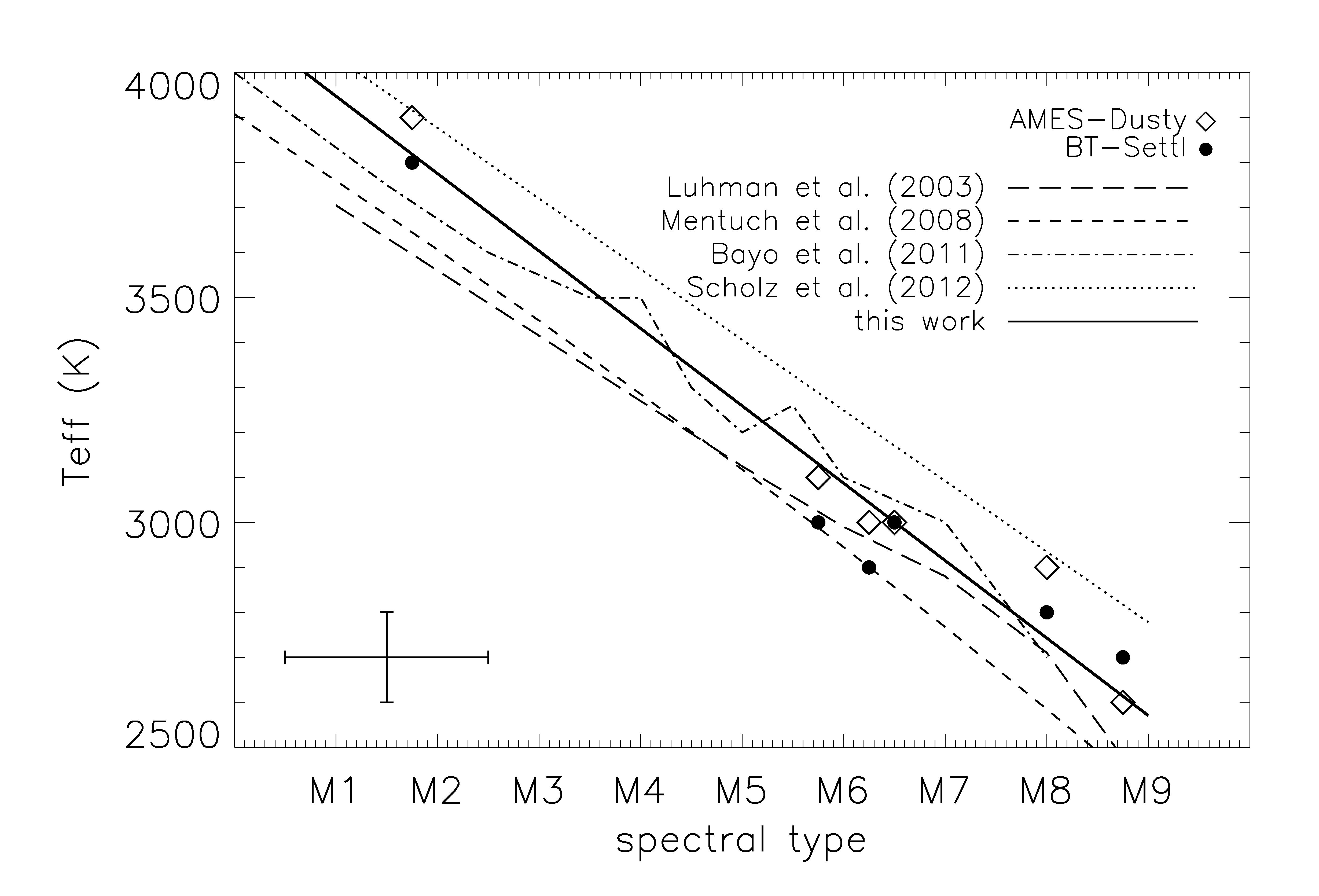
Figure 12: Comparison between the spectral types and effective temperatures for the probable members of Lupus 3 with $T_{\mathrm{eff}}<4000\,$K confirmed in this work. Two sets of symbols stand for effective temperature that were determined by fitting different models to our spectra (see Table 3). The typical error-bar is shown in the lower left corner of the plot. The solid line is a linear fit to the data points. We also show the effective temperature scales by Luhman et al. (2003b); Mentuch et al. (2008); Bayo et al. (2011); Scholz et al. (2012b).

In Figure 12, we plot the relation between $T_{\mathrm{eff}}$ and the spectral type for the objects classified as members of Lupus 3 and with $T_{\mathrm{eff}}<4000\,$K (SONYC-Lup3-1, 3, 4, 5, 7, and 10). The upper limit in $T_{\mathrm{eff}}$ is set because our spectral type fitting scheme does not extend to spectral types earlier than M1. Each object listed as member in Table 4.4 is represented by two data points, one for the $T_{\mathrm{eff}}$ derived using BT-Settl models (filled circles), and the other using AMES-Dusty (open diamonds). The solid line represents a linear fit to all the data points:

$$T_{\mathrm{eff}}=(4120\pm 175)-(172\pm 26)\times\mathrm{SpT},$$ (2)

where SpT corresponds to the M subtype. A linear least-square fit is performed using the $fitexy$ procedure from Press et al. (2002), which takes into account both the uncertainties in spectral type and $T_{\mathrm{eff}}$, shown in the lower left corner of Figure 12. The reduced $\chi^{2}$ of the fit is $2$, with the $q$ parameter of 0.996. We also show the effective temperature scales available from other works. The long-dashed line shows the scale from Luhman et al. (2003b) derived for IC348, while the dashed line represents the scale derived for the nearby young stellar associations by Mentuch et al. (2008). The latter scale is extrapolated below 3000 K. Dash-dotted line shows the scale derived from the spectroscopic data of Collinder 69 (Bayo et al., 2011), and the dotted line is a scale for NGC1333, derived by using the H-band peak index (HPI) defined in Scholz et al. (2012b). This scale was extrapolated to the spectral types earlier than M6, since the HPI index is defined only for later spectral types. We note that the scale of Scholz et al. (2012b) was derived from the near-infrared data, while all the rest are based on optical spectroscopy.

Although the trend seen in our data is generally consistent with all the previous works, some systematic offsets between the classification schemes is evident. The HPI index seems to give systematically later spectral types for a given $T_{\mathrm{eff}}$ in comparison to other schemes. The same trend was already reported in the Mužić et al. (2012), where we used the HPI to derive spectral types from NIR spectra in highly extincted cluster $\rho$ Oph. There we speculated that the extinction might introduce additional uncertainties to spectral type derived from the HPI, because the index was defined on a sample of VLMOs in NGC 1333, a cluster with A_V typically below 5. Lupus 3, however, has extinction levels comparable to those of NGC 1333, while we observe the same trend towards later spectral types. It seems therefore that for HPI the trend persist irrespective of differences in extinction of the samples, and wavelength ranges used for spectral classification (optical versus NIR). A widely-used relation between spectral type and $T_{\mathrm{eff}}$ from Luhman et al. (2003b) seems to deliver systematically lower $T_{\mathrm{eff}}$ for the same spectral type, compared to the relation derived here, especially for spectral types earlier than M6.

5.2 Census of very low-mass members of Lupus 3

The most recent summary of the population of the Lupus star forming region appeared in Comerón (2008). Since then, however, various studies have identified new low-mass members, and most importantly, there have been a significant efforts to provide spectroscopic confirmation of photometrically identified candidates. We therefore think it timely to create a summary of the previous studies, together with results of our work, and provide a census of the very low-mass content of Lupus 3. In Table Substellar Objects in Nearby Young Clusters (SONYC) VIII: Substellar population in Lupus 3, we list coordinates, photometry, spectral type and/or $T_{\mathrm{eff}}$, and alternative names for all spectroscopically confirmed members with the spectral type M0 or later. Since we choose to concentrate only on the spectroscopically confirmed members, we do not include the photometric candidates from the studies such as Nakajima et al. (2000) and López Martí et al. (2005), although we do include the identifiers from the latter study, in case they were spectroscopically confirmed in other works.

The starting point for this section is the review paper on the content of the Lupus clouds by Comerón (2008). Table 11 of the review contains a list of all classical T Tauri stars in Lupus 3 known to the date of publication. This list includes all the bright members identified and confirmed in studies by The (1962), Schwartz (1977), Krautter (1992), Hughes et al. (1994), and Krautter et al. (1997), among which are 33 M-type stars.

Comerón et al. (2003) surveyed a small area ($\sim 10^{\prime}\times 5^{\prime}$) surrounding the two brightest members HR5999 and HR6000, using slitless spectroscopy followed by the MOS follow-up using FORS/VLT. They find four M-type members, including Par-Lup3-1 (SONYC-Lup3-5), which the authors label a bona-fide BD because of the assigned spectral type of M7.5, and presence of the signatures of youth. Our spectral classification assigns it a slightly earlier spectral type (M6.25). The difference in the spectral types might arise from the different spectral typing schemes, especially since the typing in Comerón et al. (2003) was done by comparison with the field stars from Kirkpatrick et al. (1991), as not many young, low-gravity BDs were known at the time. The $T_{\mathrm{eff}}$ derived from the model fitting is, on the other hand, in excellent agreement with $2800\pm 200$ K derived from the SED modeling in the optical and near-infrared in Comerón et al. (2009).

Allen et al. (2007) spectroscopically confirmed six candidate members selected from $Spitzer$ MIR photometry, one of which was also in our high-priority selection box (SONYC-Lup3-7). Allen et al. (2007) classify SONYC-Lup3-7 as M8, in agreement with the spectral type obtained in this work.

Merín et al. (2008) selected 124 candidate members in Lupus 3 from the $c2d$ Spitzer IRAC observations. Part of this sample (46 objects) was spectroscopically followed-up with FLAMES/VLT, by Mortier et al. (2011). From the 46 objects, 8 are discarded as non-members because they lie far above the PMS evolutionary tracks. For the three objects found below the tracks, the authors propose an envelope or a edge-on disk geometry in case of membership in Lupus. Otherwise, these would be sources located in the background. One of these three objects is a well known underluminous member of Lupus 3 (Sz 102), and an emitter of forbidden lines (see Section 4.7 for more details). We choose to include one of the two remaining objects to the compiled list of members (M-65), since it exhibits MIR excess, H_α emission, and spectral type later than M0. The third object is classified as K2 (M-71) and thus not included in the census table.

Two of the spectroscopically confirmed objects from Mortier et al. (2011) are found within our photometric selection box, and for one of them we also obtained a spectrum. This is SONYC-Lup3-5 (Par-Lup3-1), which Mortier et al. classify as M5.5. In this work the same object is classified as M6.25, and by Comerón et al. (2003) M7.5. Spectra used in Mortier et al. (2011) span only the blue part of our spectral range (6550-7150 Å), which might be the cause of the different spectral classification, as the molecular features at $\lambda>7200$Å show more dramatic change with spectral type than the blue portion of the optical spectra.

Comerón et al. (2009) identified 72 candidate members of Lupus 3 with $T_{\mathrm{eff}}<3400\,$K. Recently, a spectroscopic follow-up of 46 out of 72 candidate members by Comerón et al. (2013) revealed that about 50% of the objects are background giants. Only 4 objects from the sample of Comerón et al. (2009) are in the SONYC area, and not affected by saturation and data reduction artifacts in our optical images. One of these 4 objects (16:09:20.8, -38:45:10) appears elongated in both MOSAIC and NEWFIRM images, and thus did not end up in our final $iJ$ catalog. Its spectrum by Comerón et al. (2013) shows that it is probably an M-type field dwarf. The remaining 3 objects are all found in our high-priority candidate list (photometric and proper motion selection), 2 of which were observed spectroscopically and indeed confirmed as members (SONYC-Lup3-3 and -4).

Recently, Alcalá et al. (2014) published the VLT/X-Shooter spectroscopy of several Class II YSOs in Lupus 3, selected from the lists of Merín et al. (2008) and Allen et al. (2007). Due to the exceptionally wide wavelength range of X-shooter spectra (UV to NIR), and their resolution, we expect that the spectral types derived from these observations should be highly reliable, and are included in the census in Table Substellar Objects in Nearby Young Clusters (SONYC) VIII: Substellar population in Lupus 3.

5.3 Substellar population in Lupus 3

Based on the survey presented in this work, we can put limits on the number of VLM sources that are missing in the current census of YSOs in Lupus 3. To avoid a possible bias towards the objects with disks, we base the following discussion only on the $IJ$ candidate list, and take into account only the objects above the completeness limit of our survey (dotted line in Figure 2). The completeness limit of $i=20.3$ is equivalent to 0.009 - 0.02 M_⊙ for Av=0-5, at a distance of 200 pc and age of 1 Myr, according to the BT-Settl models. The limits translate to 0.007 - 0.02 M_⊙ in case of AMES-Dusty, and 0.005 - 0.015 M_⊙ in case of AMES-COND models .

In the candidate selection box in Figure 2 we find 342 candidates above the completeness limit. Of these, 54 are also proper motion candidates (i.e., belong to the “$IJ$-pm” list). We obtained 111 spectra for the photometrically selected candidates, from which 31 are also proper motion candidates. The 7 objects confirmed to be Lupus 3 members in this work are all from the proper-motion selection. To this we add three previously confirmed members found inside the box (green stars in Figure 2), from which one is a proper-motion candidate.

Our experiment is an example of a random variable, following the binomial probability distribution. Based on the observed number of success counts in our sample, we can determine the maximum-likelihood value for the frequency of substellar objects in the sample, which is basically the ratio between the confirmed objects and those objects with spectra. The 95% confidence intervals (CI) are calculated using the Clopper-Pearson method, which is suitable for small-number events, and returns conservative CIs compared to other methods (Gehrels, 1986; Brown et al., 2001) The success rate in the “$IJ$-pm” sample is therefore $8/32=25\begin{subarray}{c}+18\\ -14\end{subarray}\%$, while for the photometric candidates it is $2/82\approx 2\begin{subarray}{c}+6\\ -2\end{subarray}\%$. In total, the estimated number of unconfirmed members in our survey is $(54-32)\times 0.25+(342-54-82)\times 0.02=6+5=11$, with the 95% CI of $\begin{subarray}{c}+13\\ -5\end{subarray}$. We can repeat the same calculation to get an approximate number of missing BD above the completeness limit. From the SONYC sources, 3 are most probably BDs (all existing spectral classifications $\geq\,$M6), while two have spectral types around the substellar border. Among the three sources from other works, one is a star earlier than M0, one is classified as M7.5 (J16083304-3855224 in Table Substellar Objects in Nearby Young Clusters (SONYC) VIII: Substellar population in Lupus 3), and the remaining one is classified as M6 (M-66). The total number of spectroscopically confirmed BDs in our sample of 342 low mass candidates above the completeness limit is therefore between 4 and 7, and only M-66 does not come from the proper motion selection. The calculation for missing BDs is identical to the one above, but with different success rates. For the “$IJ$-pm” sample we have 4 to 6 BDs over 32 objects, and for the photometric candidates 0 to 1 BD over 82. The estimated number of unconfirmed BDs is then $6\begin{subarray}{c}+10\\ -3\end{subarray}$.

5.4 Spectral type distribution

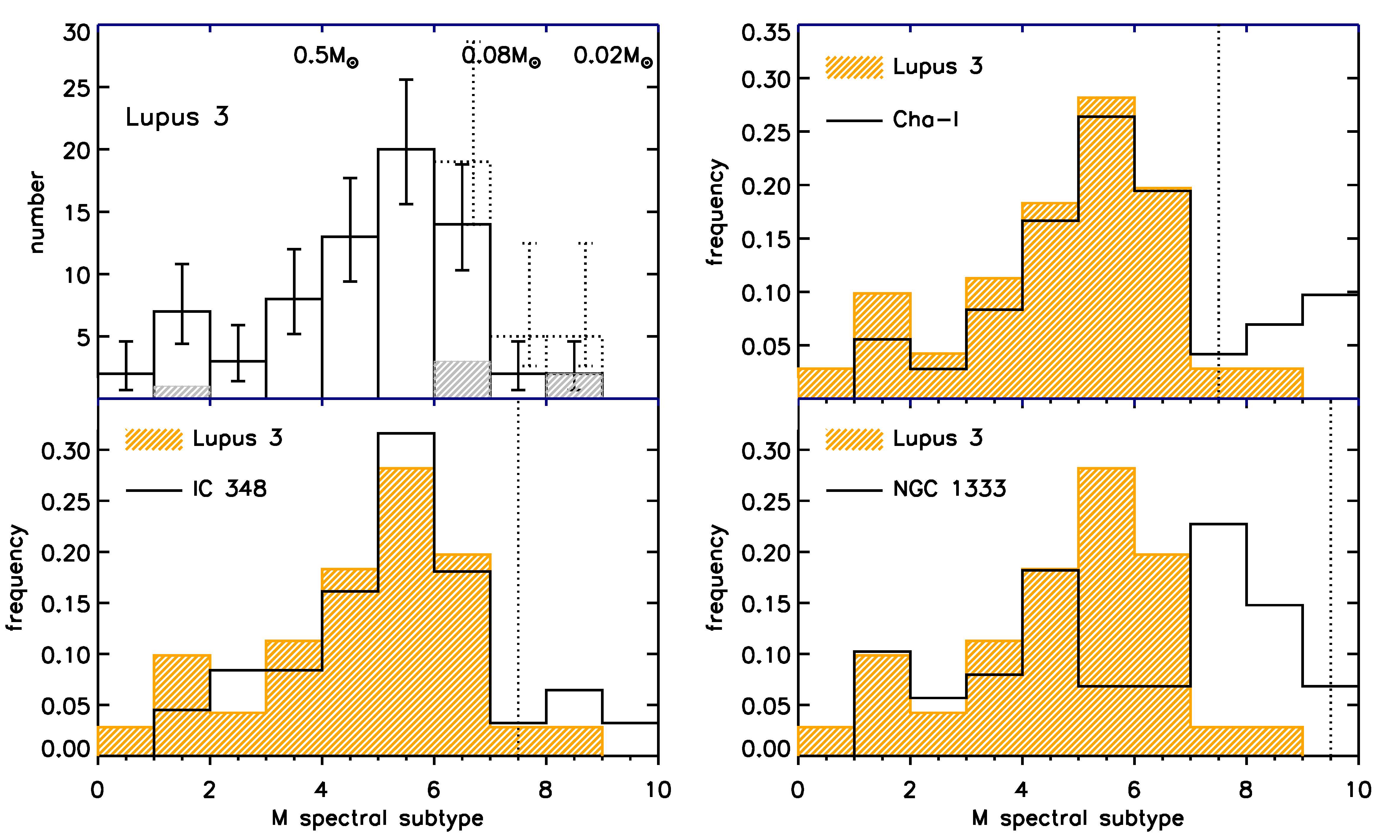
Figure 13: Top left: Distribution of spectral types for the VLM population of Lupus 3, featuring the M-type sources from Table Substellar Objects in Nearby Young Clusters (SONYC) VIII: Substellar population in Lupus 3 within the field covered by our survey. Shaded histogram shows the SONYC contribution to the census. Dotted bins take into account the estimate of the objects probably missing in our survey (for clarity, the associated error-bars are displaced to the right of the uncertainty in the number of confirmed sources). The rough mass limits according to BT-Settl and AMES-Dusty isochrones are shown on top of the plot. Top right and two bottom panels: Comparison between the spectral type distribution in Lupus 3 and those in Cha-I, IC 348 (Luhman, 2007) and NGC 1333 (Scholz et al., 2012b).

In Figure 13 we show the distribution of spectral types for the spectroscopically confirmed M-type population in Lupus 3, found within the field covered by our survey (top left panel; solid lines). The solid error bars are Poissonian confidence intervals calculated with the method described in Gehrels (1986), and the dashed histogram shows the contribution of our survey to the census. The dotted histogram includes the estimate on the number of missing objects estimated in Section 5.3, assuming that 6 of the objects are BDs (i.e. found somewhere in the last two bins, and equally distributed for the purpose of this plot), and the remaining 5 are probably low-mass stars, which due to the saturation limit of our survey around 0.06 M_⊙, should fall in the bin above. The dotted-line errorbars combine in quadrature the CI from the binomial distribution, with the errorbars shown with solid lines.

We also show a comparison with the results from other star forming regions: Cha-I (Luhman 2007; top right), IC 348 (Luhman 2007; bottom left), and NGC 1333 (Scholz et al. 2012a; lower right). In the stellar regime, the distribution resembles those seen in other star forming regions, with the peak around M5-M6, and an increase in the number of objects between M0-M1 and M5 by a factor of 2-3. Cha-I and IC 348 show a drop in the number of objects in the substellar regime with respect to stars, and this is at a similar level seen also in Lupus 3. Although this sharp drop at spectral types M7 and later can partially be explained by the incompleteness of our survey at lowest masses, it is likely to be a real feature of the IMF considering the analysis of the missing objects in our survey presented in the previous section.

In NGC 1333 (Scholz et al., 2012a), we see a second peak around M7, which might be due to a gap in the completeness between two different spectroscopic samples that were used in the stellar and substellar regimes, causing us to miss the objects around M6. The double peak is also seen in the distribution of absolute J-magnitudes, but this distribution is consistent, within statistical errors, with a single broad peak. On the substellar side, the SONYC survey in NGC 1333 is deeper than the surveys in Cha-I, IC 348 and Lupus 3, and the completeness limit is in fact outside the $x$-axis range in Figure 13. From the statistical analysis in the previous section, given the relatively large errors, we can say that the SpT distribution down to M9 is consistent with that of NGC 1333.

5.5 Star/BD ratio

In this section we use the results of our survey, combined with previous works to get some constraints on the IMF in Lupus 3, extending down to the completeness limit of our $iJ$ catalog. In the following, we will take into account the area of our combined $iJ$ survey (solid line in Figure 2). We note that the number of missing objects calculated in the previous section is partially based on the success rates of the candidates selected from the proper motions, i.e. from a somewhat smaller area than that of the photometric survey. We, however, choose not to apply any correction to account for this because, from Figure 2, it is evident that the majority of the high-priority candidates concentrate in the cloud core, and very few candidate members are expected to be missed in the surroundings. The surveys of Merín et al. (2008) and Comerón et al. (2009) have a comparable sky coverage in the area around the main Lupus 3 core, and they also cover the northeastern clouds of lower density, that are also considered to be part of the complex. This portion of the cloud contains a lower concentration of members (only about 10% of all the members identified in Merín et al. 2008 and Comerón et al. 2009), and thus excluding it should not significantly affect our analysis.

For this calculation, we compile a list of all members and candidate members from the two most extensive surveys found in the literature, Merín et al. (2008) and Comerón et al. (2009), and combine it with the sources identified in this work. As for the other works, we note that almost all sources from Table 11 of Comerón (2008) and Comerón et al. (2003), and all the confirmed sources by Allen et al. (2007), are already included either in the Merin et al. list, or the SONYC list. We also include the estimated number of still undiscovered stellar and substellar members of Lupus 3, as determined in the previous section.

Mortier et al. (2011) confirm $\sim 83\%$ of the MIR excess sources from Merín et al. (2008) as probable members of Lupus 3, while the confirmation rate for the Comerón et al. (2009) sample is $\sim 50\%$ (Comerón et al., 2013). These factors are taken into account when estimating the total number of probable members of the two mentioned studies. Another important correction factor that has to be taken into account is the disk fraction, which, according to Merín et al. (2008), is 70-80% for Lupus. Therefore, the number of objects from this work is additionally multiplied by a factor of 1.25. The sample from Merín et al. (2008) is complete down to 0.1M_⊙, and nicely complements the one of Comerón et al. (2009), whose method is only sensitive to the objects cooler than 3400 K. The 3$\sigma$ detection limit of Comerón et al. (2009) is at $I_{C}=22.2$, but the completeness limits are not specified. However, given the depth of their observations, it is probably safe to assume that they are complete in the range of masses between 0.1M_⊙ of Merín et al. (2008), and the upper limit in mass set by saturation in our optical data ($\sim$0.06 M_⊙).

To assess the numbers of stars and BDs, we use the approach described in Scholz et al. (2013). In short, by comparing the multi-band photometry with the predictions of the evolutionary models (BT-Settl in this case), we derive best-fit mass and A_V for each object, for the assumed distance of 200pc, age of 1 Myr, and the extinction law from Cardelli et al. (1989) with R${}_{V}=4$. We note that the several underluminous objects identified here and in previous studies are erroneously identified by this procedure as BDs. However, these are clearly stars, and therefore are counted in this higher-mass bin.

All the objects with estimated masses below 0.065 M_⊙ are counted as BDs, and all those above 0.085 M_⊙ as stars. The remaining objects at the border of the substellar regime are once included in the higher mass bin, and then in the lower mass bin. The calculated number of stars is then 80 - 92, and the number of BDs is estimated to be 28 - 40. Finally, we obtain the star/BD ratio between 2.0 and 3.3, in line with other star-forming regions, which typically show a span of values between 2 and 6 (Scholz et al., 2013, in press). Clearly, there is a number of uncertainties involved in this calculation due to possible incompleteness at the overlap of the different studies, uncertainties in age and distance, as well as the choice of the isochrones used to derive masses. It is nevertheless an useful exercise at least for a first order comparison with other works.

6 Summary and conclusions

In this work, we have presented deep optical and near-infrared images of the 1.4 deg² area surrounding the two brightest members HR5999/6000 of the Lupus 3 star forming region. From the optical+NIR photometry we selected 409 candidate VLM cluster members. Proper motion analysis, based on two epochs of imaging separated by 11-12 years, helped to narrow down the candidate selection to 59 high priority candidates. To confirm the membership of the selected candidates, we performed spectroscopic follow-up using VIMOS/VLT, in which we collected 123 spectra from the photometric selection box, including 32 from the high priority list. We confirm 7 candidates as probable members of Lupus 3, among which 4 are later than M6.0 and with $T_{\mathrm{eff}}\leq 3000\,$K, i.e. are probably substellar in nature. Two of the sources identified as probable members of Lupus 3 appear underluminous for their spectral class, similar to some previously known members exhibiting similar emission line spectra with strong H_α and several forbidden lines associated with active accretion.

We derive a relation between the spectral types (from comparison to low-gravity objects in young regions) and $T_{\mathrm{eff}}$ (from BT-Settl models): $T_{\mathrm{eff}}$ = $4083-166$ $\times$ SpT, where SpT refers to the M spectral subtype between 1 and 9. The rms-error of the fit of 61 K. We derive a star-to-BD ratio of 2.0 - 3.3, consistent with the values observed in other star forming regions.

Combining our results with previous work on Lupus 3, we compile a table containing all spectroscopically confirmed low-mass objects with spectral type M0 or later, and show that the distribution of spectral types is in line with what is observed in other young star forming regions.

Appendix A Model fitting plots

Figures 14 and 15 show the best-fit models from the BT-Settl and AMES-Dusty series to the spectra of the objects from Table 4.4. The results are summarized in Table 3. For more details please refer to Section 4.4.

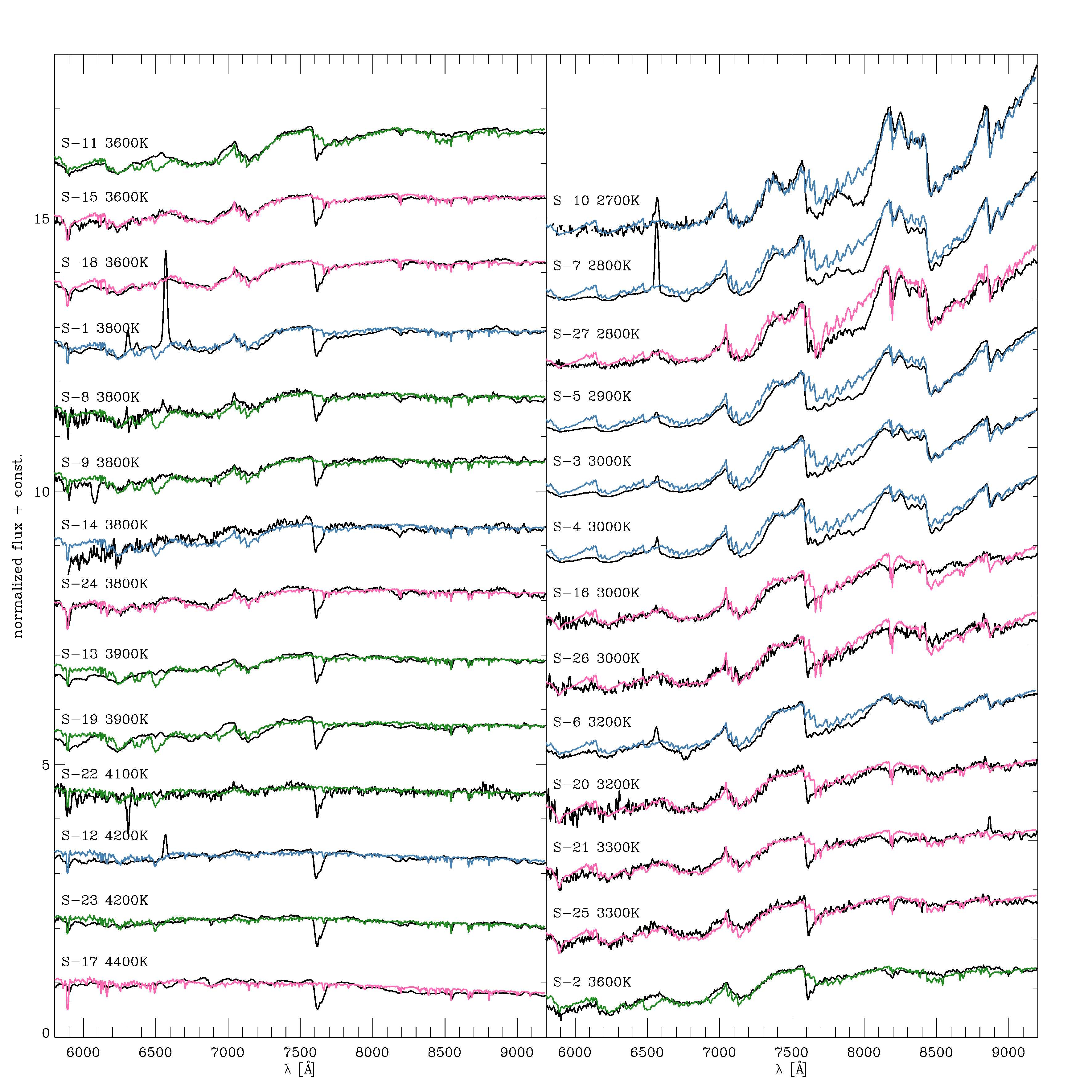
Figure 14: Spectra of the objects in Table 4.4 (black), and the best-fit BT-Settl model (Allard et al. 2011). The model spectra are color-coded according on the log$\,(g)$ used in fitting: green assume log$\,(g)=3.0$, blue log$\,(g)=3.5$, and pink log$\,(g)=5.0$. The spectral resolution of the models has been reduced by boxcar smoothing, in order to match the resolution of our spectra. Each spectrum has been corrected for extinction, but not for the atmospheric absorption.

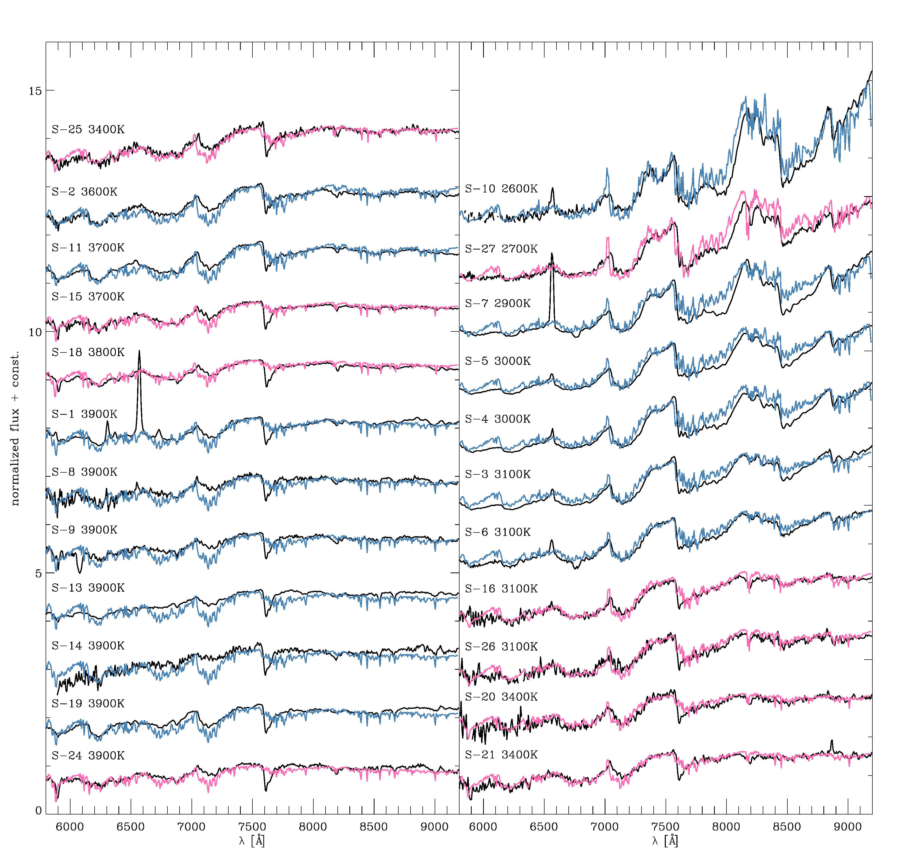
Figure 15: Spectra of the objects in Table 4.4 (black), and the best-fit AMES-Dusty model (green; Allard et al. 2001). The model spectra are color-coded according on the log$\,(g)$ used in fitting, with blue for the low-gravity objects with log$\,(g)=3.5$ or log$\,(g)=4.0$, and pink for the high-gravity objects with log$\,(g)=5.0$. The spectral resolution of the models has been reduced by boxcar smoothing, in order to match the resolution of our spectra. Each spectrum has been corrected for extinction, but not for the atmospheric absorption. Note that the AMES-Dusty model do not extend above $T_{\mathrm{eff}}=4000\,$K, therefore the hottest objects in our sample are not shown in this plot.

Table 4: Spectroscopically confirmed very low-mass members of Lupus 3

ID	$\alpha$(J2000)	$\delta$(J2000)	$J$	$K$	SpT	$T_{\mathrm{eff}}$	other names
			(mag)	(mag)		(K)
SONYC-Lup3-1	16 07 08.55	-39 14 07.8	14.6	11.5	M1.75a	3850a, 4400b	$\cdots$
SONYC-Lup3-3	16 07 55.18	-39 06 04.0	13.5	11.4	M 5.75a, M6.5c	3050a, 2900b, 2950c	$\cdots$
SONYC-Lup3-4	16 08 04.76	-39 04 49.6	13.9	12.4	M 6.50a, M7c	3000a, 2700b, 2900c	$\cdots$
SONYC-Lup3-5	16 08 16.03	-39 03 04.5	12.5	11.1	M 6.25a, M7.5d,M5.5g	2950a, 2800b	Par-Lup3-1
SONYC-Lup3-7	16 08 59.53	-38 56 27.8	13.9	12.7	M 8.00a,e, M8.5h	2850a, 2600b,h	$\cdots$
SONYC-Lup3-10	16 09 13.43	-38 58 04.9	16.1	14.9	M 8.75a	2650a	$\cdots$
SONYC-Lup3-12	16 11 18.47	-39 02 58.2	15.1	13.3	$<$M 1a	4200a	$\cdots$
EX Lup	16 03 05.5	-40 18 26	9.7	8.5	M0f	$\cdots$	HD 325367, Th 14
Sz-88	16 07 00.61	-39 02 19.9	9.9	8.6	M1f, M0h	3850h	Th 15
Sz-91	16 07 11.57	-39 03 47.2	11.1	9.8	M0.5f, M1h	3705h	Th 20
Sz-94	16 07 49.68	-39 04 28.6	11.4	10.6	M4f, M4.5g	$\cdots$	$\cdots$
Sz-95	16 07 52.29	-38 58 05.6	11.0	10.0	M1.5f	$\cdots$	$\cdots$
Sz-96	16 08 12.48	-39 08 33.0	10.1	9.0	M1.5f ,M2g	3560g	$\cdots$
Sz-97	16 08 21.84	-39 04 21.4	11.2	10.2	M3f,M4.5g, M4h	3198g, 3270h	Th 24
Sz-98	16 08 22.44	-39 04 46.7	9.5	8.0	M0f	$\cdots$	$\cdots$
Sz-99	16 08 24.00	-39 05 49.2	11.9	10.7	M3.5f,M4g,h	3270g,h	Th 25
Sz-100	16 08 25.76	-39 06 01.2	11.0	9.9	M5d,f, M4.5g, M5.5h	3198g, 3057h	Th 26
Sz-101	16 08 28.37	-39 05 32.3	10.4	9.4	M4.5g,M4f	3198g	Th 27
Sz-103	16 08 30.24	-39 06 10.8	11.4	10.2	M4f,h, M4.5g	3198g, 3270h	Th 29
Sz-104	16 08 30.72	-39 05 48.5	11.7	10.7	M5f,h,M5.5g	3058g, 3125h	Th 30
Sz-105	16 08 37.03	-40 16 20.8	9.0	7.6	M4f	$\cdots$	Th 31
Sz-106	16 08 39.76	-39 06 25.3	11.7	10.1	M0f,M2.5d, M0.5h	3777h	$\cdots$
Sz-107	16 08 41.76	-39 01 36.8	11.2	10.3	M5.5f, M6.5g	2935g	$\cdots$
Sz-108A	16 08 42.74	-39 06 18.4	9.8	8.8	M3d	$\cdots$	$\cdots$
Sz-108B	16 08 42.87	-39 06 14.6	$\cdots$	$\cdots$	M6d, M5.5g	3058g	$\cdots$
Sz-109	16 08 48.16	-39 04 19.3	11.4	10.5	M5.5f, M6.5d	$\cdots$	$\cdots$
Sz-110	16 08 51.57	-39 03 17.7	11.0	9.7	M4.5d, M3g, M2f,M4h	3415g, 3270h	Th 32
Sz-111	16 08 54.74	-39 37 43.6	10.6	9.5	M1.5f, M1h	3705h	Th 33
Sz-112	16 08 55.53	-39 02 34.0	11.0	10.0	M4f,M6d, M5h	3125h	$\cdots$
Sz-113	16 08 57.80	-39 02 22.8	12.5	11.3	M4f, M6d, M1.5g, M4.5h	3633g, 3197h	Th 34, Lup 609s
Sz-114	16 09 01.85	-39 05 12.4	10.4	9.3	M5.5d, M4g,f, M4.8h	3270g, 3175h	Th 35
Sz-115	16 09 06.23	-39 08 51.9	11.3	10.4	M4f, M4.5h	3197h	$\cdots$
Sz-116	16 09 42.61	-39 19 41.5	10.5	9.5	M1.5f	$\cdots$	Th 36
Sz-117	16 09 44.34	-39 13 30.4	10.7	9.4	M2f	$\cdots$	Th 37
Sz-119	16 09 57.07	-38 59 47.6	10.4	9.4	M4f	$\cdots$	Th 38
Sz-121	16 10 12.21	-39 21 18.6	10.0	9.0	M3f	$\cdots$	Th 40
Sz-122	16 10 16.44	-39 08 05.4	10.9	9.9	M2f	$\cdots$	Th 41
Sz-123	16 10 51.49	-38 53 14.1	11.1	9.8	M1f,h	3705h	Th 42
Par-Lup3-2	16 08 35.78	-39 03 47.9	11.2	10.3	M6d, M5g	$\cdots$	$\cdots$
Par-Lup3-3	16 08 49.40	-39 05 39.3	11.4	9.5	M4.5d, M4h	3270h	$\cdots$
Par-Lup3-4	16 08 51.44	-39 05 30.5	15.5	13.3	M5d, M4.5h	3197h	$\cdots$
Lup 713s	16 07 37.73	-39 21 38.8	13.2	12.1	M5.75e, M5.5h	3057h	$\cdots$
Lup 604s	16 08 00.17	-39 02 59.5	12.1	11.1	M5.25e, M5.5g,h	3058g,h	$\cdots$
J16081497-3857145	16 08 14.97	-38 57 14.5	15.2	13.1	M4.75e	$\cdots$	$\cdots$
Lup 706	16 08 37.33	-39 23 10.9	15.2	13.8	M7.75e, M7.5h	2795h	$\cdots$
J16085373-3914367	16 08 53.73	-39 14 36.7	15.0	12.5	M5.5e	$\cdots$	$\cdots$
M-7	16 08 55.20	-38 48 48.2	13.0	12.0	M3g	3415g	$\cdots$
M-17	16 08 28.08	-39 13 09.8	13.7	12.4	M5.5g	3058g	Lup 607
M-18	16 09 08.40	-39 03 42.8	12.2	11.4	M5.5g	$\cdots$	Lup 608s
M-19	16 08 48.24	-39 09 19.4	12.9	12.0	M6g	$\cdots$	Lup 617
M-20	16 09 49.92	-38 49 02.6	15.4	14.4	M3.5g	$\cdots$	Lup 650
M-23	16 09 17.04	-39 27 09.7	13.5	12.7	M4.5g	$\cdots$	Lup 710
M-24	16 07 58.80	-39 24 34.9	12.6	11.6	M6g	$\cdots$	Lup 714
M-25	16 11 51.12	-38 51 05.0	13.3	12.3	M5.5g	$\cdots$	Lup 802s
M-27	16 09 56.40	-38 59 51.0	13.0	12.0	M6g,h	2990g,h	Lup 818s
M-51	16 11 59.76	-38 23 38.4	12.2	11.2	M6g, M5h	2990g, 3125h	SST-Lup3-1
M-58	16 07 03.84	-39 11 11.4	14.7	13.1	M5.5g	3058g	$\cdots$
M-62	16 09 01.44	-39 25 12.0	11.6	10.3	M3.5g, M4h	3343g, 3270h	$\cdots$
M-65	16 10 12.96	-38 46 16.3	15.9	13.9	M4g	3270g	$\cdots$
M-66	16 10 19.92	-38 36 06.5	13.3	12.3	M6g	2990g	$\cdots$
M-67	16 10 29.52	-39 22 14.5	11.9	10.9	M5.5g	3058g	$\cdots$
M-69	16 11 31.92	-38 11 10.0	12.3	10.7	M2.5g	3488g	$\cdots$
M-70	16 11 44.88	-38 32 44.9	12.4	11.5	M6.5g	2935g	$\cdots$
J16052862-3846210	16 05 28.63	-38 46 21.1	12.6	11.8	M6c	3000c	$\cdots$
J16083304-3852224	16 08 33.05	-38 52 22.4	12.9	11.9	M7.5c	2800c	$\cdots$
J16083547-3900358	16 08 35.48	-39 00 35.8	11.5	10.6	M6.5c	2950c	$\cdots$
J16083974-3929228	16 08 39.75	-39 29 22.9	11.7	10.9	M5c	3100c	$\cdots$
J16085575-3826330	16 08 55.75	-38 26 33.1	13.0	12.1	M5.5c	3050c	$\cdots$
J16090452-3921125	16 09 04.52	-39 21 12.5	10.7	9.8	M5c	3100c	$\cdots$
J16091570-3851396	16 09 15.71	-38 51 39.7	12.0	11.2	M5c	3100c	$\cdots$
J16092279-3855506	16 09 22.80	-38 55 50.6	10.8	9.9	M5c	3100c	J160922.8-385550Ac
J16092320-3855547	16 09 23.20	-38 55 54.8	10.8	9.9	M4c	3250c	J160922.8-385550Bc
J16092800-3848538	16 09 28.01	-38 48 53.8	11.9	11.0	M5.5c	3050c	$\cdots$
J16101386-3759589	16 10 13.87	-37 59 58.9	12.2	11.2	M6c	3000c	$\cdots$
J16103062-3831517	16 10 30.62	-38 31 51.7	13.3	12.4	M6c	3000c	$\cdots$
J16103323-3830234	16 10 33.23	-38 30 23.5	10.8	9.8	M4.5c	3200c	$\cdots$
J16104192-3823046	16 10 41.92	-38 23 04.7	10.9	10.0	M5c	3100c	$\cdots$
J16105899-3914514	16 10 58.99	-39 14 51.4	12.1	11.3	M5c	3100c	$\cdots$
J16113801-3841356	16 11 38.02	-38 41 35.7	10.9	10.1	M2.5c	3500c	$\cdots$
J16120761-3813242	16 12 07.61	-38 13 24.3	10.9	10.0	M4.5c	3200c	$\cdots$
J16121046-3909040	16 12 10.46	-39 09 04.0	13.9	12.8	M6.5c	2950c	$\cdots$
J16122559-3817428	16 12 25.58	-38 17 42.8	13.1	12.2	M6c	3000c	$\cdots$

Note. — Identifiers are from Schwartz (1977, Sz), Comerón et al. (2003, Par-Lup3), López Martí et al. (2005, Lup), Mortier et al. (2011, M), and 2MASS (J16).

References. — (a) this work, (b) Comerón et al. (2009), (c) Comerón et al. (2013), (d) Comerón et al. (2003), (e) Allen et al. (2007), (f) Hughes et al. (1994), (g) Mortier et al. (2011), (h) Alcalá et al. (2014).

References

- Alcalá et al. (2014) Alcalá, J. M., Natta, A., Manara, C. F., et al. 2014, A&A, 561, A2
- Allard et al. (2001) Allard, F., Hauschildt, P. H., Alexander, D. R., Tamanai, A., & Schweitzer, A. 2001, ApJ, 556, 357
- Allard et al. (2011) Allard, F., Homeier, D., & Freytag, B. 2011, in Astronomical Society of the Pacific Conference Series, Vol. 448, 16th Cambridge Workshop on Cool Stars, Stellar Systems, and the Sun, ed. C. Johns-Krull, M. K. Browning, & A. A. West, 91
- Allen et al. (2004) Allen, L. E., Calvet, N., D’Alessio, P., et al. 2004, ApJS, 154, 363
- Allen et al. (2007) Allen, P. R., Luhman, K. L., Myers, P. C., et al. 2007, ApJ, 655, 1095
- Allers et al. (2006) Allers, K. N., Kessler-Silacci, J. E., Cieza, L. A., & Jaffe, D. T. 2006, ApJ, 644, 364
- Baade et al. (1999) Baade, D., Meisenheimer, K., Iwert, O., et al. 1999, The Messenger, 95, 15
- Baraffe et al. (1998) Baraffe, I., Chabrier, G., Allard, F., & Hauschildt, P. H. 1998, A&A, 337, 403
- Baraffe et al. (2009) Baraffe, I., Chabrier, G., & Gallardo, J. 2009, ApJ, 702, L27
- Barrado y Navascués & Martín (2003) Barrado y Navascués, D. & Martín, E. L. 2003, AJ, 126, 2997
- Bastian et al. (2010) Bastian, N., Covey, K. R., & Meyer, M. R. 2010, ARA&A, 48, 339
- Bayo et al. (2011) Bayo, A., Barrado, D., Stauffer, J., et al. 2011, A&A, 536, A63
- Bayo et al. (2008) Bayo, A., Rodrigo, C., Barrado Y Navascués, D., et al. 2008, A&A, 492, 277
- Bertout et al. (1999) Bertout, C., Robichon, N., & Arenou, F. 1999, A&A, 352, 574
- Bessell & Brett (1988) Bessell, M. S. & Brett, J. M. 1988, PASP, 100, 1134
- Bonnell et al. (2007) Bonnell, I. A., Larson, R. B., & Zinnecker, H. 2007, Protostars and Planets V, 149
- Brown et al. (2001) Brown, L. D., Cai, T. T., & Dasgupta, A. 2001, Statistical Science, 16, 101
- Cambrésy (1999) Cambrésy, L. 1999, A&A, 345, 965
- Cardelli et al. (1989) Cardelli, J. A., Clayton, G. C., & Mathis, J. S. 1989, ApJ, 345, 245
- Chabrier et al. (2000) Chabrier, G., Baraffe, I., Allard, F., & Hauschildt, P. 2000, ApJ, 542, 464
- Chapman et al. (2007) Chapman, N. L., Lai, S.-P., Mundy, L. G., et al. 2007, ApJ, 667, 288
- Comerón (2008) Comerón, F. The Lupus Clouds, ed. B. Reipurth, 295
- Comerón (2011) —. 2011, A&A, 531, A33
- Comerón et al. (2003) Comerón, F., Fernández, M., Baraffe, I., Neuhäuser, R., & Kaas, A. A. 2003, A&A, 406, 1001
- Comerón et al. (2009) Comerón, F., Spezzi, L., & López Martí, B. 2009, A&A, 500, 1045
- Comerón et al. (2013) Comerón, F., Spezzi, L., López Martí, B., & Merín, B. 2013, A&A, 554, A86
- Epchtein et al. (1994) Epchtein, N., de Batz, B., Copet, E., et al. 1994, Ap&SS, 217, 3
- Fernández & Comerón (2005) Fernández, M. & Comerón, F. 2005, A&A, 440, 1119
- Geers et al. (2011) Geers, V., Scholz, A., Jayawardhana, R., et al. 2011, ApJ, 726, 23
- Gehrels (1986) Gehrels, N. 1986, ApJ, 303, 336
- Gondoin (2006) Gondoin, P. 2006, A&A, 454, 595
- Hartmann (1998) Hartmann, L. 1998, Accretion Processes in Star Formation
- Horne (1986) Horne, K. 1986, PASP, 98, 609
- Huélamo et al. (2010) Huélamo, N., Bouy, H., Pinte, C., et al. 2010, A&A, 523, A42
- Hughes et al. (1993) Hughes, J., Hartigan, P., & Clampitt, L. 1993, AJ, 105, 571
- Hughes et al. (1994) Hughes, J., Hartigan, P., Krautter, J., & Kelemen, J. 1994, AJ, 108, 1071
- Jeffries (2012) Jeffries, R. D. 2012, in EAS Publications Series, Vol. 57, EAS Publications Series, ed. C. Reylé, C. Charbonnel, & M. Schultheis, 45–89
- Kirkpatrick et al. (1991) Kirkpatrick, J. D., Henry, T. J., & McCarthy, Jr., D. W. 1991, ApJS, 77, 417
- Kirkpatrick et al. (1995) Kirkpatrick, J. D., Henry, T. J., & Simons, D. A. 1995, AJ, 109, 797
- Krautter (1986) Krautter, J. 1986, A&A, 161, 195
- Krautter (1992) —. The Star Forming Region in Lupus, ed. B. Reipurth, 127
- Krautter et al. (1997) Krautter, J., Wichmann, R., Schmitt, J. H. M. M., et al. 1997, A&AS, 123, 329
- Lombardi et al. (2008) Lombardi, M., Lada, C. J., & Alves, J. 2008, A&A, 480, 785
- López Martí et al. (2005) López Martí, B., Eislöffel, J., & Mundt, R. 2005, A&A, 440, 139
- López Martí et al. (2011) López Martí, B., Jiménez-Esteban, F., & Solano, E. 2011, A&A, 529, A108
- Luhman (2004a) Luhman, K. L. 2004a, ApJ, 602, 816
- Luhman (2004b) —. 2004b, ApJ, 616, 1033
- Luhman (2004c) —. 2004c, ApJ, 617, 1216
- Luhman (2007) —. 2007, ApJS, 173, 104
- Luhman et al. (2003a) Luhman, K. L., Briceño, C., Stauffer, J. R., et al. 2003a, ApJ, 590, 348
- Luhman et al. (2003b) Luhman, K. L., Stauffer, J. R., Muench, A. A., et al. 2003b, ApJ, 593, 1093
- Makarov (2007) Makarov, V. V. 2007, ApJ, 658, 480
- Martín et al. (1999) Martín, E. L., Delfosse, X., Basri, G., et al. 1999, AJ, 118, 2466
- Mentuch et al. (2008) Mentuch, E., Brandeker, A., van Kerkwijk, M. H., Jayawardhana, R., & Hauschildt, P. H. 2008, ApJ, 689, 1127
- Merín et al. (2007) Merín, B., Augereau, J.-C., van Dishoeck, E. F., et al. 2007, ApJ, 661, 361
- Merín et al. (2008) Merín, B., Jørgensen, J., Spezzi, L., et al. 2008, ApJS, 177, 551
- Mortier et al. (2011) Mortier, A., Oliveira, I., & van Dishoeck, E. F. 2011, MNRAS, 418, 1194
- Mužić et al. (2011) Mužić, K., Scholz, A., Geers, V., Fissel, L., & Jayawardhana, R. 2011, ApJ, 732, 86
- Mužić et al. (2012) Mužić, K., Scholz, A., Geers, V., Jayawardhana, R., & Tamura, M. 2012, ApJ, 744, 134
- Nakajima et al. (2000) Nakajima, Y., Tamura, M., Oasa, Y., & Nakajima, T. 2000, AJ, 119, 873
- Osterbrock (1989) Osterbrock, D. E. 1989, Astrophysics of gaseous nebulae and active galactic nuclei
- Pecaut & Mamajek (2013) Pecaut, M. J. & Mamajek, E. E. 2013, ArXiv e-prints
- Pontoppidan et al. (2007) Pontoppidan, K. M., Stapelfeldt, K. R., Blake, G. A., van Dishoeck, E. F., & Dullemond, C. P. 2007, ApJ, 658, L111
- Press et al. (2002) Press, W. H., Teukolsky, S. A., Vetterling, W. T., & Flannery, B. P. 2002, Numerical recipes in C++ : the art of scientific computing
- Riddick et al. (2007) Riddick, F. C., Roche, P. F., & Lucas, P. W. 2007, MNRAS, 381, 1067
- Schlieder et al. (2012) Schlieder, J. E., Lépine, S., & Simon, M. 2012, AJ, 144, 109
- Schödel et al. (2009) Schödel, R., Merritt, D., & Eckart, A. 2009, A&A, 502, 91
- Scholz et al. (2007) Scholz, A., Coffey, J., Brandeker, A., & Jayawardhana, R. 2007, ApJ, 662, 1254
- Scholz et al. (2013) Scholz, A., Geers, V., Clark, P., Jayawardhana, R., & Muzic, K. 2013, ApJ, 775, 138
- Scholz et al. (2009) Scholz, A., Geers, V., Jayawardhana, R., et al. 2009, ApJ, 702, 805
- Scholz et al. (2012a) Scholz, A., Jayawardhana, R., Muzic, K., et al. 2012a, ApJ, 756, 24
- Scholz et al. (2012b) Scholz, A., Muzic, K., Geers, V., et al. 2012b, ApJ, 744, 6
- Schwartz (1977) Schwartz, R. D. 1977, ApJS, 35, 161
- Skrutskie et al. (2006) Skrutskie, M. F., Cutri, R. M., Stiening, R., et al. 2006, AJ, 131, 1163
- Stelzer et al. (2013) Stelzer, B., Frasca, A., Alcalá, J. M., et al. 2013, A&A, 558, A141
- Strauss et al. (1992) Strauss, M. A., Huchra, J. P., Davis, M., et al. 1992, ApJS, 83, 29
- Tachihara et al. (2007) Tachihara, K., Rengel, M., Nakajima, Y., et al. 2007, ApJ, 659, 1382
- The (1962) The, P.-S. 1962, Contributions from the Bosscha Observervatory, 15, 0
- West et al. (2008) West, A. A., Hawley, S. L., Bochanski, J. J., et al. 2008, AJ, 135, 785
- White & Basri (2003) White, R. J. & Basri, G. 2003, ApJ, 582, 1109
- Wichmann et al. (1998) Wichmann, R., Bastian, U., Krautter, J., Jankovics, I., & Rucinski, S. M. 1998, MNRAS, 301, L39
- Wood et al. (2002) Wood, K., Wolff, M. J., Bjorkman, J. E., & Whitney, B. 2002, ApJ, 564, 887