Matrix Bases for Star Products: a Review

Matrix Bases for Star Products: a Review

Fedele LIZZI ^†‡§ and Patrizia VITALE ^†‡

F. Lizzi and P. Vitale

^† Dipartimento di Fisica, Università di Napoli Federico II, Napoli, Italy fedele.lizzi@na.infn.it, patrizia.vitale@na.infn.it

^‡ INFN, Sezione di Napoli, Italy ^§ Institut de Ciéncies del Cosmos, Universitat de Barcelona, Catalonia, Spain

Received March 04, 2014, in final form August 11, 2014; Published online August 15, 2014

We review the matrix bases for a family of noncommutative $\star$ products based on a Weyl map. These products include the Moyal product, as well as the Wick–Voros products and other translation invariant ones. We also review the derivation of Lie algebra type star products, with adapted matrix bases. We discuss the uses of these matrix bases for field theory, fuzzy spaces and emergent gravity.

noncommutative geometry; star products; matrix models

58Bxx; 40C05; 46L65

1 Introduction

Star products were originally introduced [34, 62] in the context of point particle quantization, they were generalized in [9, 10] to comprise general cases, the physical motivations behind this was the quantization of phase space. Later star products became a tool to describe possible noncommutative geometries of spacetime itself (for a review see [4]). In this sense they have become a tool for the study of field theories on noncommutative spaces [77]. In this short review we want to concentrate on one particular aspect of the star product, the fact that any action involving fields which are multiplied with a star product can be seen as a matrix model. This is because the noncommutative star products algebras can always be represented as operators on a suitable Hilbert space, and one can then just consider the matrix representation of these operators. The matrix representation is not only a useful tool, but also offers a conceptual interpretation of noncommutative spaces. It shows that, in analogy with quantum phase space, the proper setting of deformed products is noncommutative geometry [20], seen as a spectral theory of operators.

This is a partial review, as we do not have the ambition to cover exhaustively all known products, nor all known bases. We will consider products which are connected to symmetries and which have developments in field theory. Even then we will not cover completely all work done, and apologize for the omissions.

In order to construct the matrix bases we will use mainly quantization-dequantization maps, whereby we associate operators to functions, and viceversa. We will first consider a family of translation-invariant star products induced on suitable algebras of functions on ${\mathbb{R}}^{2n}$ through $s$-ordered quantization-dequantization maps. In this approach noncommutative algebras are obtained as symbols of algebras of operators, which are defined in terms of a special family of operators using the trace formula (what is sometimes called the ‘dequantization’ map because of its original meaning in the Wigner–Weyl formalism), while the reconstruction of operators in terms of their symbols (the ‘quantization’ map) is determined using another family of operators. These two families determine completely the noncommutative algebra, including the kernel of the star-product.

Once we have established the connection, in Section 4 we construct matrix bases for $s$-ordered products and for the Moyal and Wick–Voros cases in more detail. In Section 5 we review the construction of a family of star products of Lie algebra type, obtained by reduction of higher-dimensional, translation invariant ones. We thus discuss in Section 6 the matrix basis for one of them on the space ${\mathbb{R}}^{3}$. Section 7 is devoted to the application to quantum field theory of the matrix bases introduced previously. Finally, Section 8 is devoted to fuzzy spaces.

2 The star product

In this section we review a general construction for the noncommutative algebra of operator symbols acting on a Hilbert space $\mathcal{H}$. We follow the presentation and the notation of [56, 57].

Given an operator $\hat{A}$ acting on the Hilbert space $\mathcal{H}$ (which can be finite- or infinite-dimensional), let us have two distinct operator bases for the operators acting on ${\mathcal{H}}$, $\hat{U}(x)$ and $\hat{D}(x)$. The two bases are labelled by a set of parameters $x=(x_{1},\dots,x_{N})$, with $x_{k}\in\mathbb{K}$, $k=1,\dots,N$, with $\mathbb{K}$ any field, usually the reals, complex or integers. The symbol $f_{A}(x)$ of the operator $\hat{A}$ is the following function of $x$:

$$f_{A}=\Omega^{-1}\big{(}\hat{A}\big{)}\equiv\operatorname{tr}\big{(}\hat{A}\hat{U}(x)\big{)}.$$ (2.1)

We assume that the trace exists for all parameters $x$, although often the function $f$ may be a distribution. If we now consider the “parameters” $x$ as the coordinates of a manifold it makes sense to define the inverse map (the “reconstruction formula”), which associates operators to functions, is defined in terms of the second family of operators, that is

$$\hat{A}=\hat{\Omega}(f_{A})=\int f_{A}(x)\hat{D}(x){\mathrm{d}}x.$$ (2.2)

The map $\hat{\Omega}$ is often called the quantization map, because of its role in quantum mechanics. In the standard quantization scheme, which associates Hermitian operators to real functions, it is the Weyl map, whereas its inverse is the Wigner map. We assume that an appropriate measure ${\mathrm{d}}x$ exists to make sense of the reconstruction formula and that the two maps have a sufficiently rich domain to ensure that the maps are invertible for a dense set in the space of functions. In this way we have an invertible map between functions on space and operators on a Hilbert space.

The symbols form an associative algebra endowed with a noncommutative (star) product defined in terms of the operator product

$$f_{A}\star f_{B}(x)=\Omega^{-1}\big{(}\hat{A}\hat{B}\big{)}=\operatorname{tr}\big{(}\hat{A}\hat{B}\hat{U}(x)\big{)},$$ (2.3)

where the associativity follows from the associativity of the operator product.

The star product may be expressed in terms of an integral kernel

$$f_{A}\star f_{B}(x)=\int f_{A}(x^{\prime})f_{B}(x^{\prime\prime})K(x^{\prime},x^{\prime\prime},x){\mathrm{d}}x^{\prime}{\mathrm{d}}x^{\prime\prime},$$ (2.4)

with

$$K(x^{\prime},x^{\prime\prime},x)=\operatorname{tr}\big{(}\hat{D}(x^{\prime})\hat{D}(x^{\prime\prime})\hat{U}(x)\big{)}.$$ (2.5)

The operators $\hat{D}(x)$ and $\hat{U}(x)$ are also known as quantizer and dequantizer. The associativity condition implies

$$\int K(x^{\prime},y,x)K(x^{\prime\prime},x^{\prime\prime\prime},y){\mathrm{d}}y=\int K(x^{\prime},x^{\prime\prime},y)K(y,x^{\prime\prime\prime},x){\mathrm{d}}y.$$

From the compatibility request of equations (2.1), (2.2) we easily derive an important condition that the two families of basic operators have to satisfy

$$\operatorname{tr}\big{(}\hat{D}(x^{\prime})\hat{U}(x)\big{)}=\delta(x^{\prime}-x),$$ (2.6)

where $\delta$ is to be replaced with the Kronecker delta for discrete parameters. Going back to (2.5), it is to be stressed that the kernel of the star product has been obtained solely in terms of the operators $D(x)$ and $U(x)$, which in turn are only constrained by (2.6). Thus, to each pair of operators satisfying (2.6) it is associated an associative algebra with a star product. The role of $D(x)$ and $U(x)$ can be exchanged, what gives rise to a duality symmetry [56]. This duality allows for the definition of a new star product, different from the one in (2.4) (unless $\hat{U}$ and $\hat{D}$ are proportional), defined in terms of a dual kernel

$$K^{d}(x^{\prime},x^{\prime\prime},x)=\operatorname{tr}\big{(}\hat{U}(x^{\prime})\hat{U}(x^{\prime\prime})\hat{D}(x)\big{)}.$$

3 The Weyl–Wigner and the $\boldsymbol{s}$-ordered maps

In this section we review the usual Moyal product on the two-dimensional plane ${\mathbb{R}}^{2}$ and the family of $s$-ordered products which generalizes it. The generalization is made in terms of the quantization-dequantization maps illustrated above.

We first review a few properties of coherent states and their relation to the number basis, which shall be used in the rest of this section. Let $x=(x_{1},x_{2})\in{\mathbb{R}}^{2}$. We use a slightly unconventional notation for the coordinates on the complex plane defining:

$$z=\frac{1}{\sqrt{2}}(x_{1}+{\mathrm{i}}x_{2}).$$

We define the creation and annihilation operators on the plane, $a^{\dagger}$, $a$, as

$$a^{\dagger}=\frac{1}{\sqrt{2}}(\hat{x}_{1}-{\mathrm{i}}\hat{x}_{2}),\qquad a=\frac{1}{\sqrt{2}}(\hat{x}_{1}+{\mathrm{i}}\hat{x}_{2})$$

with commutation relation

$$[a,a^{\dagger}]=\theta,$$

where $\theta$ is a dimensional parameter of area dimension. Coherent states of the plane are thus defined by $a|z\rangle=z|z\rangle$. The decomposition of the identity reads

$$\mathbf{1}=\frac{1}{\pi\theta}\int{\mathrm{d}}^{2}z|z\rangle\langle z|.$$

Coherent states are non-orthogonal

$$\langle z|z^{\prime}\rangle={\mathrm{e}}^{-\frac{1}{\theta}(\bar{z}z+\bar{z}^{\prime}z^{\prime}-2\bar{z}z^{\prime})}.$$

Given the number operator $\hat{N}=a^{\dagger}a$, and indicating with $|n\rangle$ its eigenvalues, we state the useful relations

$$a|n\rangle=\sqrt{n\theta}|n-1\rangle,\qquad a^{\dagger}|n\rangle=\sqrt{(n+1)\theta}|n+1\rangle,\qquad|n\rangle=\frac{\big{(}a^{\dagger}\big{)}^{n}}{\sqrt{n!\theta^{n}}}|0\rangle$$ (3.1)

together with

$$\langle z|n\rangle={\mathrm{e}}^{-\frac{\bar{z}z}{2\theta}}\frac{\bar{z}^{n}}{\sqrt{n!\theta^{n}}}.$$

3.1 The Moyal product

Given an operator $\hat{A}$ acting in the Hilbert space of square integrable functions on ${\mathbb{R}}$, the Wigner–Weyl symbol of $\hat{A}$ and the reconstruction map are defined by means of the families of operators

$$\hat{U}_{\rm M}(x)=2~{}\hat{\mathcal{D}}(z,\bar{z})(-\hat{1})^{a^{\dagger}a}\hat{\mathcal{D}}(-z,-\bar{z}),$$ (3.2)

$$\hat{D}_{\rm M}(x)={1\over(2\pi)^{2}}\hat{U}_{\rm M}(x),$$ (3.3)

where $(-\hat{1})^{a^{\dagger}a}$ is the parity operator. To simplify notations we assume $\theta=1$ unless otherwise stated. $\hat{\mathcal{D}}(z,\bar{z})$ is the unitary displacement operator realizing the ray representation of the group of translations of the plane

$$\hat{\mathcal{D}}(z,\bar{z})={\rm e}^{za^{\dagger}-\bar{z}a},\qquad\hat{\mathcal{D}}(z,\bar{z})|w\rangle=|w+z\rangle{\rm e}^{\frac{1}{2}(z\bar{w}-w\bar{z})}.$$ (3.4)

We shall use the isomorphism ${\mathbb{R}}^{2}={\mathbb{C}}$ in the following and the notation $\hat{\mathcal{D}}(z)$ as a shorthand for $\hat{\mathcal{D}}(z,\bar{z})$ to indicate the functional dependence on the plane coordinates from now on.

The compatibility condition (2.6) between the operators (3.2) and (3.3) is then readily verified on using well known properties of $\hat{\mathcal{D}}(z)$

$$(-\hat{1})^{a^{\dagger}a}\hat{\mathcal{D}}(z)(-\hat{1})^{a^{\dagger}a}=\hat{\mathcal{D}}(-z),\qquad\operatorname{tr}\hat{\mathcal{D}}(z)=\pi\delta({\rm Re}~{}z)\delta(\operatorname{Im}z).$$ (3.5)

The quantizer and dequantizer may be expressed in the more familiar form

$$\hat{D}_{\rm M}(x)=\frac{1}{(2\pi)^{2}}\hat{U}_{\rm M}(x)=\int\frac{{\mathrm{d}}^{2}\xi}{(2\pi)^{2}}\exp\big{[}{\mathrm{i}}\big{(}\xi_{1}(\hat{x}_{2}-x_{2})+\xi_{2}(\hat{x}_{1}-x_{1})\big{)}\big{]}.$$ (3.6)

The Weyl quantization map obtained by the reconstruction formula (2.2) therefore reads

$$\hat{\Omega}(f)=\hat{f}=\int{\mathrm{d}}^{2}xf(x)\int\frac{{\mathrm{d}}^{2}\xi}{(2\pi)^{2}}\exp\big{[}{\mathrm{i}}\big{(}\xi_{1}(\hat{x}_{2}-x_{2})+\xi_{2}(\hat{x}_{1}-x_{1})\big{)}\big{]},$$

whereas the inverse map obtained by (2.2) is represented by:

$$f(x)=\operatorname{tr}\left(\hat{f}\int{\mathrm{d}}^{2}\xi\exp\big{[}{\mathrm{i}}\big{(}\xi_{1}(\hat{x}_{2}-x_{2})+\xi_{2}(\hat{x}_{1}-x_{1})\big{)}\big{]}\right).$$

The algebra of symbols so defined is endowed with the well known Moyal product. In this language it is defined in terms of the kernel, which is easily obtained specializing (2.5) to this case. On restoring the noncommutative parameter $\theta$ and using the first of equations (3.5) together with the product rule for the displacement operators

$$\hat{\mathcal{D}}(z)\hat{\mathcal{D}}(z^{\prime})=\hat{\mathcal{D}}(z+z^{\prime}){\mathrm{e}}^{{\mathrm{i}}\operatorname{Im}(z\bar{z}^{\prime})}$$

we have indeed

$$K_{\rm M}(x^{\prime},x^{\prime\prime},x)=C\exp\big{\{}{2{\mathrm{i}}}\epsilon^{ij}\big{[}x_{i}x^{\prime}_{j}+x^{\prime}_{i}x^{\prime\prime}_{j}+x^{\prime\prime}_{i}x_{j}\big{]}\big{\}}$$ (3.7)

with $C$ a normalization constant and $\epsilon^{ij}$ the antisymmetric tensor. Its expression in complex coordinates is also useful for future comparison

$$K_{\rm M}(z^{\prime},z^{\prime\prime},z)=C\exp\big{\{}4{\mathrm{i}}\operatorname{Im}\big{[}\bar{z}^{\prime}z^{\prime\prime}+z\bar{z}^{\prime\prime}+z^{\prime}\bar{z}\big{]}\big{\}}.$$ (3.8)

The Moyal product is then defined as

$$(f\star_{\rm M}g)(x)=\int{{\mathrm{d}}^{2}x^{\prime}}{{\mathrm{d}}^{2}x^{\prime\prime}}f(x^{\prime})g(x^{\prime\prime})K_{\rm M}(x^{\prime},x^{\prime\prime},x).$$ (3.9)

In complex coordinates the relation (3.9) reads

$$(f\star_{\rm M}g)(z,\bar{z})=\int{\mathrm{d}}^{2}z^{\prime}{\mathrm{d}}^{2}z^{\prime\prime}f(z^{\prime},\bar{z}^{\prime})g(z^{\prime\prime},\bar{z}^{\prime\prime}){\mathrm{e}}^{\{{4{\mathrm{i}}}\operatorname{Im}[\bar{z}^{\prime}z^{\prime\prime}+z\bar{z}^{\prime\prime}+z^{\prime}\bar{z}]\}}.$$

In the case of the coordinate functions on $\mathbb{R}^{2}$, upon restoring the factors of $\theta$, this gives the usual star-commutation relation

$$[x_{1},x_{2}]_{\star_{\rm M}}={\mathrm{i}}\theta$$ (3.10)

or equivalently

$$[z,\bar{z}]_{\star_{\rm M}}=\theta.$$ (3.11)

The Moyal product can be given the popular form

$$(f\star_{\rm M}g)(z,\bar{z})=f(z,\bar{z})\exp\left[\frac{\theta}{2}\big{(}\overleftarrow{\partial_{z}}\overrightarrow{\partial_{\bar{z}}}-\overleftarrow{\partial_{\bar{z}}}\overrightarrow{\partial_{z}}\big{)}\right]g(z,\bar{z}),$$ (3.12)

where the operator $\overleftarrow{\partial}$ (resp. $\overrightarrow{\partial}$) acts on the left (resp. on the right). It is well known that this form is obtained by the integral expression through an asymptotic expansion in the parameter $\theta$ [25].

The generalization to the higher-dimensional cases is straightforward.

What is properly defined as the Moyal algebra is $\mathcal{M}_{\theta}:=\mathcal{M}_{L}({{\mathbb{R}}}_{\theta}^{2})\cap\mathcal{M}_{R}({{\mathbb{R}}}_{\theta}^{2})$ where $\mathcal{M}_{L}({{\mathbb{R}}}_{\theta}^{2})$, the left multiplier algebra, is defined as the subspace of tempered distributions that give rise to Schwartz functions when left multiplied by Schwartz functions; the right multiplier algebra $\mathcal{M}_{R}({{\mathbb{R}}}_{\theta}^{2})$ is analogously defined. For more details we refer to the appendix in [32] and references therein. In the present article we can think of $\mathcal{M}_{\theta}$ either as the algebra of $\star$-polynomial functions in $z$, $\bar{z}$ properly completed, or the algebra generated by Schwarz functions, or a variant. One should however pay attention since the domains of definition depend on the particular form of the product. Its commutative limit, $\mathcal{F}({\mathbb{R}}^{2})$, is the commutative multiplier algebra $\mathcal{O}_{\rm M}({\mathbb{R}}^{2})$, the algebra of smooth functions of polynomial growth on ${\mathbb{R}}^{2}$ in all derivatives [29].

3.2 $\boldsymbol{s}$-ordered symbols

$s$-ordered symbols have been introduced long ago by Cahill and Glauber [16] in the context of quantum mechanics to deal with different orderings w.r.t. the Weyl–Wigner symmetric ordering of operators. The corresponding quantization and dequantization maps are often referred to as weighted maps. We refer to [57] and references therein for more details. Here the stress will be on the different star-products which are related to such orderings. We consider the two families of operators $\hat{U}_{s}(x)$ and $\hat{D}_{s}(x)$, $x\in{\mathbb{R}}^{2}$, of the form [16]

$$\hat{U}_{s}(x)={2\over(1+s)}\hat{\mathcal{D}}(z)\left({s-1\over s+1}\right)^{a^{\dagger}a}\hat{\mathcal{D}}(-z)=\frac{2}{1+s}\left(\frac{s-1}{s+1}\right)^{(a^{\dagger}-\bar{z})(a-z)},$$ (3.13)

$$\hat{D}_{s}(x)={1\over(2\pi)^{2}}\hat{U}_{-s}(x),$$ (3.14)

where $s$ is chosen to be real in the analysis below. We shall see that the convergence of the kernel will impose constraints on the allowed values of $s$. The case $s=0$ corresponds to the standard Wigner–Weyl situation described above. Two other relevant cases correspond to the singular limits $s=\pm 1$ which yield respectively normal and anti-normal ordering in quantization. It is interesting to notice that these two cases are in the duality relation discussed previously (namely the role of $\hat{U}$ and $\hat{D}$ are exchanged). The duality symmetry then connects normal and anti-normal ordering. The Wigner–Weyl Moyal quantization scheme selects instead the symmetric ordering, consistently with it being self-dual.

For $s\neq\pm 1$ the star-product kernel of $s$-ordered symbols is calculated along the same lines as the Moyal kernel (3.7). To our knowledge it was first calculated in [56], although no analysis on the convergence was made. Let us sketch the derivation. For simplicity we define $q=(s+1)/(s-1)$, $\tilde{q}=q^{-1}$ and we skip overall constants. From the definition (2.5) and the dequantizer and quantizer operators (3.13), (3.14), we have

$$K_{s}(z^{\prime},z^{\prime\prime},z)=\operatorname{tr}\big{(}\hat{D}(\bar{z}^{\prime},z^{\prime})\hat{D}(\bar{z}^{\prime\prime},z^{\prime\prime})\hat{U}(\bar{z},z)\big{)}=(1-q)^{2}(1-\tilde{q})$$

$$\qquad\times\operatorname{tr}\big{(}\hat{\mathcal{D}}(-\bar{z},-z)\hat{\mathcal{D}}(\bar{z}^{\prime},z^{\prime})q^{a^{\dagger}a}\hat{\mathcal{D}}(-\bar{z}^{\prime},-z^{\prime})\hat{\mathcal{D}}(\bar{z}^{\prime\prime},z^{\prime\prime})q^{a^{\dagger}a}\hat{\mathcal{D}}(-\bar{z}^{\prime\prime},-z^{\prime\prime})\hat{\mathcal{D}}(\bar{z},z){\tilde{q}}^{a^{\dagger}a}\big{)}.$$

Let us introduce

$$x=-z+z^{\prime},\qquad y=-z^{\prime}+z^{\prime\prime}\qquad\text{so that}\qquad-z^{\prime\prime}+z=-x-y.$$ (3.15)

On using the composition rule for the generalized displacement operator $\hat{\mathcal{D}}(\bar{w},z)={\rm{exp}}(za^{\dagger}-\bar{w}a)$

$$\hat{\mathcal{D}}(\bar{w},z)\hat{\mathcal{D}}(\bar{u},y)=\hat{\mathcal{D}}(\bar{w}+\bar{u},z+y)\exp\big{(}\tfrac{1}{2}(z\bar{u}-y\bar{w})\big{)}$$

and the commutation relation

$$q^{a^{\dagger}a}\hat{\mathcal{D}}(\bar{z},z)=\hat{\mathcal{D}}(\tilde{q}\bar{z},qz)q^{a^{\dagger}a},$$

we arrive at

$$K_{s}(z^{\prime},z^{\prime\prime},z)=K_{s}(x,y)=(1-q)(1-\tilde{q})^{2}\operatorname{tr}\big{[}\hat{\mathcal{D}}((1-\tilde{q})\bar{x},(1-q)x)q^{a^{\dagger}a}\big{]}$$

$$\hphantom{K_{s}(z^{\prime},z^{\prime\prime},z)=}{}\times\exp\big{[}(1-q)\bar{x}y-(1-\tilde{q})\bar{y}x-\tfrac{1}{2}(q-\tilde{q})\bar{x}x\big{]}.$$ (3.16)

On using the coherent states basis to compute the trace, we have

$$q^{a^{\dagger}a}|w\rangle={\rm e}^{(q^{2}-1)\frac{\bar{w}w}{2}}|qw\rangle,$$

so that we are left with a Gaussian integral

$$\operatorname{tr}\big{[}\hat{\mathcal{D}}((1-\tilde{q})\bar{x},(1-q)x)q^{a^{\dagger}a}\big{]}={\rm e}^{(\tilde{q}-q)\bar{x}x}\int{\mathrm{d}}^{2}w{\rm e}^{-(1-q)(\bar{w}-\bar{x})(w-x)}=\frac{{\rm e}^{(\tilde{q}-q)\bar{x}x}}{1-q}.$$

On replacing into equation (3.16) we finally have

$$K_{s}(x,y)=C(1-\tilde{q})(1-q){\rm e}^{(\tilde{q}-q)\bar{x}x+(1-q)\bar{x}y-(1-\tilde{q})\bar{y}x}$$ (3.17)

with $C$ an overall constant. This expression can be seen to reproduce the Moyal kernel (3.8) for $s=0$ ($q=\tilde{q}=-1$). On replacing the original variables $z$, $z^{\prime}$, $z^{\prime\prime}$, it can be seen to coincide with the result of [56], up to the exchange of $q$ with $\tilde{q}$. We have indeed

$$K_{s}(z^{\prime},z^{\prime\prime},z)=C(1-\tilde{q})(1-q){\rm exp}\big{[}(\tilde{q}-q)\bar{z}z+(\tilde{q}-1)z^{\prime}\bar{z}^{\prime\prime}+(1-q)z^{\prime\prime}\bar{z}^{\prime}+(q-1)z^{\prime\prime}\bar{z}$$

$$\phantom{K_{s}(z^{\prime},z^{\prime\prime},z)=}{}+(1-\tilde{q})z\bar{z}^{\prime\prime}+(q-1)z\bar{z}^{\prime}+(1-\tilde{q})z^{\prime}\bar{z}\big{]}.$$ (3.18)

Let us notice that this expression is singular for $s\rightarrow\pm 1$. These two cases have to be considered separately (in the following we will explicitly compute the kernel for the case $s=1$). We will denote with $\star_{s}$ the corresponding star product and with $\mathcal{A}_{s}$ the noncommutative algebra of functions on the plane with $\star_{s}$-noncommutativity, so to have

$$(f\star_{s}g)(\bar{z},z)=\int{\mathrm{d}}^{2}z^{\prime}{\mathrm{d}}^{2}z^{\prime\prime}f(\bar{z}^{\prime},z^{\prime})g(\bar{z}^{\prime\prime},z^{\prime\prime})K_{s}(z^{\prime},z^{\prime\prime},z).$$

The convergence of such an expression might impose severe constraints on the algebra of functions selected and has to be analyzed case by case. A careful analysis of the convergence of the kernel shows that its integral is finite and equal to 1 (as it should) only for $-1<s\leq 0$. Indeed the introduction of the variables $x$ and $y$ makes it clear that for such a choice of $s$ the integral of $K(x,y)$ is Gaussian.

As for series expressions of the product, analogues of (3.12) it should be possible to obtain them on restoring the noncommutative parameter and expanding in terms of it, as in the Moyal case. We are not aware that such expressions have been investigated before, but we see no a priori obstruction to perform the calculation.

To illustrate the usefulness of equation (3.17) let us compute the star product of $z$ with $\bar{z}$ in detail. We have

$$z\star_{s}\bar{z}=\int{\mathrm{d}}^{2}z^{\prime}{\mathrm{d}}^{2}z^{\prime\prime}z^{\prime}\bar{z}^{\prime\prime}K_{s}(z^{\prime},z^{\prime\prime},z).$$

On expressing $z^{\prime}$, $z^{\prime\prime}$ in terms of the variables $x$ and $y$ introduced in (3.15) and replacing the integral kernel we arrive at

$$z\star_{s}\bar{z}=(1-\tilde{q})(1-q)\int{\mathrm{d}}^{2}x{\mathrm{d}}^{2}y(x+z)(\bar{x}+\bar{y}+\bar{z}){\rm e}^{(\tilde{q}-q)\bar{x}x+(1-q)\bar{x}y-(1-\tilde{q})\bar{y}x},$$

which may be reduced to a sum of Gaussian integrals. By direct calculation we see that the integrals containing $\bar{x}x$, $\bar{x}z$, $\bar{z}x$ and $\bar{y}z$ are zero. We are left with

$$z\star_{s}\bar{z}=(1-\tilde{q})(1-q)\int{\mathrm{d}}^{2}x{\mathrm{d}}^{2}y(\bar{z}z+x\bar{y}){\rm e}^{(\tilde{q}-q)\bar{x}x+(1-q)\bar{x}y-(1-\tilde{q})\bar{y}x}.$$ (3.19)

The first integral is exactly the integral of the kernel, multiplied by the factor $\bar{z}z$

$$\int{\mathrm{d}}^{2}x{\mathrm{d}}^{2}y{\rm e}^{(\tilde{q}-q)\bar{x}x+(1-q)\bar{x}y-(1-\tilde{q})\bar{y}x}=\frac{1}{(1-q)(1-\tilde{q})}.$$ (3.20)

The second one can be seen to yield

$$\int{\mathrm{d}}^{2}x{\mathrm{d}}^{2}y\bar{y}x{\rm e}^{(\tilde{q}-q)\bar{x}x+(1-q)\bar{x}y-(1-\tilde{q})\bar{y}x}=\frac{1}{(1-q)(1-\tilde{q})^{2}}.$$ (3.21)

Thus, replacing (3.20) and (3.21) into (3.19), we obtain the interesting result

$$z\star_{s}\bar{z}=\bar{z}z+\frac{1}{1-\tilde{q}}.$$

Analogously we obtain

$$\bar{z}\star_{s}z=\bar{z}z-\frac{1}{1-q}$$

so to obtain for the star commutator

$$z\star_{s}\bar{z}-\bar{z}\star_{s}z=1,$$

which is independent of $q$ as expected (we recall that all translation-invariant products are equivalent from the point of view of the star commutator, being a quantization of the same Poisson bracket).

In this section we have chosen for simplicity to stick to $s$, hence $q$, $\tilde{q}$, real. The analysis can be repeated for $s$ complex. The convergence of the kernel and of the star product will impose constraints on the real part of $s$.

3.3 The Wick–Voros product

Let us consider the normal ordered case ($s=1$) in more detail. It has been shown [16] that in such case the limit for the quantizer is singular (its eigenvalues are infinite for all values of $z$) and we may represent it as the normal-ordered operator delta function

$$\hat{D}_{\rm W}(z)=\int{{\mathrm{d}}^{2}\xi}{\mathrm{e}}^{{\xi}(a^{\dagger}-\bar{z})}{\mathrm{e}}^{-\bar{\xi}(a-z)}$$ (3.22)

with $\xi=\xi_{1}+{\mathrm{i}}\xi_{2}$, which differs from (3.6) by a phase. Operators in such a scheme acquire the normal-ordered expression

$$\hat{f}=\sum\limits_{n,m=0}^{\infty}f_{nm}\big{(}a^{{\dagger}}\big{)}^{n}a^{m}.$$

The dequantizer instead is simply the projection operator over coherent states

$$\hat{U}_{\rm W}(z)=|z\rangle\langle z|,$$

so that the Wick–Voros star product which is associated to this quantization-dequantization scheme, can be easily computed by means of equation (2.3) in terms of the expectation value over coherent states

$$(f\star_{\rm W}g)(z,\bar{z})=\operatorname{tr}\big{(}|z\rangle\langle z|\hat{f}\hat{g}|\big{)}=\langle z|\hat{f}\hat{g}|z\rangle=\sum\limits_{n,m,p,q}f_{nm}g_{pq}\langle z|\big{(}a^{{\dagger}}\big{)}^{n}a^{m}\big{(}a^{{\dagger}}\big{)}^{p}a^{q}|z\rangle$$

$$\phantom{(f\star_{\rm W}g)(z,\bar{z})}=\int{{\mathrm{d}}^{2}\xi}\sum\limits_{n,m,p,q}f_{nm}g_{pq}\bar{z}^{n}z^{q}\langle z|a^{m}|\xi\rangle\langle\xi|\big{(}a^{{\dagger}}\big{)}^{p}|z\rangle$$

$$\phantom{(f\star_{\rm W}g)(z,\bar{z})}=\int{{\mathrm{d}}^{2}\xi}\sum\limits_{n,m,p,q}f_{nm}g_{pq}\bar{z}^{n}z^{q}\xi^{m}\bar{\xi}^{p}\langle z|\xi\rangle\langle\xi|\big{(}a^{{\dagger}}\big{)}^{p}|z\rangle$$

$$\phantom{(f\star_{\rm W}g)(z,\bar{z})}=\int{{\mathrm{d}}^{2}\xi}f(\bar{z},\xi)g(\bar{\xi},z)|\langle z|\xi\rangle|^{2}.$$ (3.23)

Alternatively, on using equation (2.5), we may compute the kernel of the star product

$$K_{\rm W}(z^{\prime},z^{\prime\prime},z)=\operatorname{tr}\big{[}\hat{D}(\bar{z}^{\prime},z^{\prime})\hat{D}(\bar{z}^{\prime\prime},z^{\prime\prime})\hat{U}(\bar{z},z)\big{]}=\langle z|\hat{D}(\bar{z}^{\prime},z^{\prime})\hat{D}(\bar{z}^{\prime\prime},z^{\prime\prime})|z\rangle$$

$$\phantom{K_{\rm W}(z^{\prime},z^{\prime\prime},z)}{}=\int{{\mathrm{d}}^{2}\xi}\langle z|\hat{D}(\bar{z}^{\prime},z^{\prime})|\xi\rangle\langle\xi|\hat{D}(\bar{z}^{\prime\prime},z^{\prime\prime})|z\rangle$$

and replace the latter in the star product expression

$$(f\star_{\rm W}g)(\bar{z},z)=\int{\mathrm{d}}^{2}z^{\prime}{\mathrm{d}}^{2}z^{\prime\prime}f(\bar{z}^{\prime},z^{\prime})g(\bar{z}^{\prime\prime},z^{\prime\prime})K_{\rm W}(z^{\prime},z^{\prime\prime},z).$$ (3.24)

On using for example the matrix basis expansion of operators equation (3.3) and the quantization map equation (2.2) we then observe that

$$f(\bar{z},\xi)\langle z|\xi\rangle=\langle z|\hat{f}|\xi\rangle=\int{\mathrm{d}}^{2}z^{\prime}f(\bar{z}^{\prime},z^{\prime})\langle z|\hat{D}(\bar{z}^{\prime},z^{\prime})|\xi\rangle,$$

which shows that equation (3.24) coincides with the direct computation obtained in (3.23).

As in the case of the Moyal product, upon restoring the parameter $\theta$ we can perform a series expansion, yielding the popular expression

$$(f\star_{\rm W}g)(z,\bar{z})=f(z,\bar{z})\exp\big{[}\theta\overleftarrow{\partial_{z}}\overrightarrow{\partial_{\bar{z}}}\big{]}g(z,\bar{z}).$$ (3.25)

The Wick–Voros product has been employed in QFT to discuss the emergence of the mixing independently from the specific translation invariant product chosen [27]. In [8] the Wick–Voros star product is singled out as it allows for a consistent definition of quantum state.

A word of caution is in order, concerning the domain and the range of the weighted Weyl map associated to the Wick–Voros quantizer (3.22). While the standard Weyl map associates to Schwarzian functions Hilbert Schmidt operators, for the weighted Weyl map determined the Wick–Voros quantizer (3.22) this is not always the case. Explicit counterexamples are discussed in [48, 49, 50, 51]. The exact correspondence between the appropriate subalgebras of smooth functions on the plane and bounded operators is discussed in [73] for all $s$-ordered quantization schemes, whereas the convergence of the series expansion in (3.25) has been extensively discussed and established in [11] and references therein.

One important aspect of these products is the fact that derivatives are inner automorphisms:

$$\frac{\partial}{\partial x^{i}}f=\theta^{-1}\varepsilon_{ij}[x^{j},f]_{\star}$$

and

$$\partial_{z}f=\theta^{-1}[f,\bar{z}]_{\star},\qquad\partial_{\bar{z}}f=\theta^{-1}[f,z]_{\star}.$$ (3.26)

Note that these relations are valid for all products considered in this section. This is a straightforward consequence of the fact that the $\star$ commutator (3.11) holds not only for the Moyal product, but for all $s$-ordered products.

3.4 Translation invariance

Defining the translation in the plane ${\mathbb{R}}^{2}$ by a vector $a$ as ${\mathcal{T}}_{a}(f)(x)=f(x+a)$, by translation invariant product we mean the property

$${\mathcal{T}}_{a}(f)\star{\mathcal{T}}_{a}(g)={\mathcal{T}}_{a}(f\star g).$$ (3.27)

It is interesting to notice that $s$-ordered star products described in the previous subsection are translation invariant. This is an almost obvious consequence of the fact that $s$-ordered star products are defined in terms of the displacement operator (3.4), which realizes a representation of the group of translations of the plane. It is however straightforward to check the relation (3.27), once we observe that the integral kernel for $s$-ordered products (3.18) verifies

$$K(z^{\prime},z^{\prime\prime},z+\xi)=K(z^{\prime}-\xi,z^{\prime\prime}-\xi,z).$$

A slightly more general form for translation invariant products of the plane, which also includes commutative ones is represented by

$$(f\star g)(x)=\frac{1}{2\pi}\int{\mathrm{d}}^{2}p{\mathrm{d}}^{2}q{\mathrm{e}}^{{\mathrm{i}}p\cdot x}\tilde{f}(q)\tilde{g}(p-q){\mathrm{e}}^{\alpha(p,q)}$$

with $\tilde{f}$, $\tilde{g}$ the Fourier transforms of $f$, $g$.

The function $\alpha$ is further restricted by the associativity request. A full analysis of the family of translation-invariant products, together with a study of the cohomology associated to them, is performed in [28, 81]. The usual pointwise product is reproduced by $\alpha=0$, the Moyal product by $\alpha_{\rm M}(p,q)=-{\mathrm{i}}/2\theta^{ij}q_{i}p_{j}$ and the Wick–Voros product by $\alpha_{\rm W}(p,q)=-\theta q_{-}(p_{+}-q_{+})$, with $q_{\pm}=\frac{q_{1}\pm{\mathrm{i}}q_{2}}{\sqrt{2}}$.

4 Matrix bases for $\boldsymbol{s}$-ordered products

In this section we consider matrix bases for the $s$-ordered star-products described in the previous sections. We shall give a unified derivation for all of them and then specialize to the known cases of the Moyal [33, 79] and Wick–Voros [49] matrix bases.

To a function on the plane $\mathbb{R}^{2}$ we associate via the quantization map (2.2) and the $s$-ordered quantizer (3.14) the $s$-ordered operator

$$\phi(z,\bar{z})\rightarrow:\hat{\phi}(a,a^{\dagger}):_{s}$$

with $:\;:_{s}$ denoting $s$-ordering. This may be expanded into $s$-ordered powers of $a$, $a^{\dagger}$

$$\hat{\phi}=\sum\limits_{p,q}\tilde{\phi}_{pq}:\big{(}a^{\dagger}\big{)}^{p}a^{q}:_{s}.$$ (4.1)

On using the number basis defined in equation (3.1) we may rewrite (4.1) as

$$\hat{\phi}=\sum\limits_{p,q}\phi^{s}_{pq}|p\rangle\langle q|$$

with $\tilde{\phi}_{pq}$, $\phi^{s}_{kl}$ related by a change of basis which depends explicitly on the ordering. On applying the dequantization formula (2.1) with the $s$-ordered dequantizer defined by equation (3.13) we obtain a function in the noncommutative algebra $\mathcal{A}_{s}$

$$\phi(z,\bar{z})=\sum\limits_{p,q}\phi^{s}_{pq}f^{s}_{pq}(z,\bar{z})$$ (4.2)

with

$$f^{s}_{pq}(z,\bar{z})=\operatorname{tr}\big{(}|p\rangle\langle q|\hat{U}_{s}(\bar{z},z)\big{)}=\frac{1}{\sqrt{p!q!\theta^{p+q}}}\operatorname{tr}\big{(}\big{(}a^{\dagger}\big{)}^{p}|0\rangle\langle 0|a^{q}\hat{U}_{s}(\bar{z},z)\big{)}.$$

By definition (cf. (2.3)) this yields $f^{s}_{pq}(z,\bar{z})$ as a star product

$$f^{s}_{pq}(z,\bar{z})=\frac{1}{\sqrt{p!q!\theta^{p+q}}}\bar{z}^{p}\star_{s}f_{00}\star_{s}z^{q}$$ (4.3)

with $f^{s}_{00}(\bar{z},z)$ the $s$-ordered symbol of the operator $|0\rangle\langle 0|$

$$f^{s}_{00}(\bar{z},z)=\operatorname{tr}\big{(}|0\rangle\langle 0|\hat{U}_{s}(\bar{z},z)\big{)}$$

and $\bar{z}^{p}$, $z^{q}$ respectively symbols of $\big{(}a^{\dagger}\big{)}^{p}$, $a^{q}$ in all schemes (equation (4.3) is thus true by definition of star product (2.3), and the use of associativity:

$$(f_{A}\star_{s}f_{B}\star_{s}f_{C})(\bar{z},z)=\operatorname{tr}\big{(}\hat{A}\hat{B}\hat{C}\hat{U}_{s}(\bar{z},z)\big{)}$$

with the identification $\hat{A}=\big{(}a^{\dagger}\big{)}^{p}$, $\hat{B}=|0\rangle\langle 0|$, $\hat{C}=a^{q}$).

It is immediate to verify that $f^{s}_{00}(\bar{z},z)$ is idempotent independently from the particular form of the operator $\hat{U}_{s}$. We have indeed

$$(f_{00}\star_{s}f_{00})(\bar{z},z)=\operatorname{tr}\big{(}|0\rangle\langle 0|0\rangle\langle 0|\hat{U}_{s}(\bar{z},z)\big{)}=f_{00}(\bar{z},z).$$

The basis elements $f_{pq}(z,\bar{z})$ may be seen to obey the following fusion rule

$$f_{pq}\star_{s}f_{kl}=\delta_{qk}f_{pl}$$ (4.4)

by observing that, by definition

$$f_{pq}\star_{s}f_{kl}=\operatorname{tr}\big{(}|p\rangle\langle q|k\rangle\langle l|\hat{U}_{s}(\bar{z},z)\big{)}.$$

This implies that every $s$-ordered star product may be described as matrix product. We have indeed

$$\phi\star_{s}\psi(\bar{z},z)=\sum\phi_{nm}\psi_{pq}f_{nm}\star_{s}f_{pq}(\bar{z},z)=\sum\phi_{nm}\psi_{mq}f_{nq}(\bar{z},z)=\sum(\Phi\cdot\Psi)_{nq}f_{nq}(\bar{z},z)$$

with $\Phi$, $\Psi$ the infinite matrices with entries the series expansion coefficients of the functions $\phi$, $\psi$ (see equation (4.2)). The idempotent function $f_{00}$ may be computed explicitly. On using the number basis $n$ and the $s$-ordered dequantizer (3.13) we have

$$\frac{(1+s)}{2}f_{00}(\bar{z},z)=\sum\limits_{n}\langle n|0\rangle\langle 0|\hat{\mathcal{D}}(z)\left({s-1\over s+1}\right)^{a^{\dagger}a}\hat{\mathcal{D}}(-z)|n\rangle$$

$$\hphantom{\frac{(1+s)}{2}f_{00}(\bar{z},z)}{}=\langle 0|\hat{\mathcal{D}}(z)\left({s-1\over s+1}\right)^{a^{\dagger}a}\hat{\mathcal{D}}(-z)|0\rangle=\sum\limits_{nm}\langle-z|n\rangle\langle n|\left({s-1\over s+1}\right)^{a^{\dagger}a}|m\rangle\langle m||-z\rangle$$

$$\hphantom{\frac{(1+s)}{2}f_{00}(\bar{z},z)}{}={\mathrm{e}}^{-\frac{\bar{z}z}{\theta}}\sum\limits_{nm}(-1)^{n+m}\frac{\bar{z}^{n}z^{m}}{\sqrt{n!m!\theta^{n+m}}}\left({s-1\over s+1}\right)^{m}\delta_{nm}={\mathrm{e}}^{-\frac{\bar{z}z}{\theta}}{\mathrm{e}}^{\frac{s-1}{s+1}\frac{\bar{z}z}{\theta}}.$$ (4.5)

As we can see, it depends explicitly on the value of $s$. This is a particular case of a more general formula [16, equations (6.35), (6.36)]. We shall see in next sections that it reproduces correctly previous results which have been obtained in specific quantization-dequantization schemes.

We can establish the useful result for the integral of the basis functions $f_{pq}$. We have

$$\int{\mathrm{d}}^{2}zf_{pq}(\bar{z},z)=\int{\mathrm{d}}^{2}z\langle q|U_{s}|p\rangle=2\pi\theta\delta_{pq}.$$ (4.6)

The generalization to four dimensions is readily obtained on introducing

$$f_{PQ}(\bar{z}_{a},z_{a})=f_{p_{1}q_{1}}(\bar{z}_{1},z_{1})\cdot f_{q_{2}p_{2}}(\bar{z}_{2},z_{2}),\qquad a=1,2.$$

Together with the fusion rule equation (4.4), equation (4.6) ensures that the matrix basis $f_{pq}(\bar{z},z)$ is orthogonal. This has the important consequence that the action of every field theory model with $s$-ordered star product becomes a matrix action, with integrals replaced by traces. To illustrate this point, let us consider for simplicity a scalar action with polynomial interaction, in two dimensions

$$S[\phi]=\int{\mathrm{d}}^{2}z(\phi\star_{s}\widehat{O}\phi)(\bar{z},z)+\lambda\phi^{\star_{s}n}(z,\bar{z})$$

with $\phi^{\star_{s}n}=\phi\star_{s}\phi\star_{s}\cdots\star_{s}\phi$ n times. On expanding the fields in the matrix basis as in in equation (4.2) we first observe that, thanks to (4.4) repeatedly applied, the star product in the algebra becomes an infinite-matrix product

$$\phi_{1}\star_{s}\phi_{2}\star_{s}\cdots\star_{s}\phi_{n}(\bar{z},z)=\sum\limits_{p_{i},q_{i}}{\phi_{1}}_{p_{1}q_{1}}{\phi_{2}}_{p_{2}q_{2}}\cdots{\phi_{n}}{p_{n}q_{n}}f_{p_{1}q_{1}}\star_{s}f_{p_{2}q_{2}}\star_{s}\cdots\star_{s}f_{p_{n}q_{n}}$$

$$\qquad={\sum\limits_{p_{1},q_{n}}(\Phi_{1}\cdot\Phi_{2}\cdots\Phi_{n})_{p_{1}q_{n}}f_{p_{1}q_{n}}},$$

where $\Phi=\{\phi_{pq}\}$ are the infinite matrices of fields coefficients in the matrix basis expansion (4.2). On integrating the latter expression by means of (4.6) we finally get

$$\int{\mathrm{d}}^{2}z{\phi_{1}\star\phi_{2}}\star\cdots\star\phi_{n}(\bar{z},z)=2\pi\theta\operatorname{tr}(\Phi_{1}\cdot\Phi_{2}\cdots\Phi_{n}).$$

For the kinetic term we proceed analogously, although it is in general not diagonal in the matrix basis. Repeating the same steps we arrive at

$$\int{\mathrm{d}}^{2}z(\phi\star_{s}\widehat{O}\phi)(\bar{z},z)=\operatorname{tr}\Phi O\Phi$$

with

$$(O)_{pq;rs}=\int{\mathrm{d}}^{2}zf_{pq}\star_{s}\widehat{O}f_{rs}$$

the representation of the kinetic operator on the matrix basis, to be computed case by case. Applications of this procedure may be found in Section 7.

4.1 The Moyal matrix basis

We have seen in previous sections that the Moyal product is introduced through a symmetric-ordered quantization scheme. When qualifying ${\mathbb{R}}^{2}$ as the phase space of 1-dimensional systems, the basis functions $f_{pq}(z,\bar{z})$ in this quantization scheme correspond exactly to the Wigner functions associated to the density operator of the quantum oscillator states.

The Moyal matrix basis has been established long ago by J.M. Gracia-Bondía and J.C. Várilly following a slightly different approach [33, 79] with respect to the one described in previous section. The idempotent function $f_{00}(\bar{z},z)$ has been shown [33, 79] to be the Gaussian

$$f^{\rm M}_{00}(\bar{z},z)=2\exp(-2\bar{z}z/\theta),$$

which agrees with our result (4.5) at $s=0$. The expression of the matrix elements $\phi_{kl}$ in terms of $\tilde{\phi}_{pq}$ has been computed for the Moyal case in [52].

The extension to $\mathbb{R}^{4}_{\theta}$ is straightforward. We have

$$\phi(z_{a},\bar{z}_{a})=\sum\limits_{PQ}\phi_{PQ}f^{\rm M}_{PQ}(z_{a},\bar{z}_{a})$$ (4.7)

with $a=1,2$, $P=(p_{1},p_{2})$ and

$$f^{\rm M}_{PQ}(z_{a},\bar{z}_{a})=f^{\rm M}_{p_{1},q_{1}}(z_{1},\bar{z}_{1})\cdot f^{\rm M}_{p_{2},q_{2}}(z_{2},\bar{z}_{2}).$$

In order to describe elements of $\mathbb{R}_{\theta}^{2}$ (resp. $\mathbb{R}_{\theta}^{4}$), the sequences $\{\phi_{pq}\}$ (resp. $\{\phi_{\vec{p}\vec{q}}\}$) have to be of rapid decay [33, 79].

4.2 The Wick–Voros matrix basis

We have seen previously that the Wick–Voros product is introduced through a weighted quantization map which, in two dimensions, associates to functions on the complex plane normal ordered operators. The inverse map which is the analogue of the Wigner map is represented by

$$\phi(z,\bar{z})=\langle z|\hat{\phi}|z\rangle.$$ (4.8)

The Wick–Voros product, $\phi\star_{\rm W}\psi$, is particularly simple with respect to the other $s$-ordered products (including the well studied Moyal one). It is defined as the expectation value over coherent states of the operator product $\hat{\phi}\hat{\psi}$. Then, for analytic functions, a very convenient way to reformulate the quantization map (2.2) is to consider the analytic expansion

$$\phi(\bar{z},z)=\sum\limits_{pq}\tilde{\phi}_{pq}\bar{z}^{p}z^{q},\qquad p,q\in\mathbb{N},$$

with $\tilde{\phi}_{pq}\in{\mathbb{C}}$. The Wick–Voros quantizer (3.22) will then produce the normal ordered operator

$$\hat{\phi}=\sum\limits_{pq}\tilde{\phi}_{pq}\big{(}a^{{\dagger}}\big{)}^{p}a^{q}.$$

We will therefore assume analyticity in what follows. The idempotent function $f_{00}$ is a Gaussian, as for the Moyal case, although with a slightly different shape

$$f^{\rm W}_{00}(\bar{z},z)=\exp(-\bar{z}z/\theta).$$

This result agrees with the general result (4.5) for $s=1$. The basis functions $f^{\rm W}_{pq}$ acquire the simple form

$$f^{\rm W}_{pq}(z,\bar{z})=\frac{{\rm e}^{-\frac{\bar{z}z}{\theta}}}{\sqrt{p!q!\theta^{p+q}}}\bar{z}^{p}z^{q},$$

where we notice that no star product is present anymore differently from what happens in all other situations described by equation (4.3) with $s\neq 1$, including the Moyal case, $s=0$. This is due to the fact that $\bar{z}^{p}\star_{\rm W}f=\bar{z}^{p}\cdot f$ as well as $f\star_{\rm W}z^{q}=f\cdot z^{q}$. The generalization to ${\mathbb{R}}^{4}$ is straightforward and follows the same lines as for the Moyal case. We have

$$f^{\rm W}_{PQ}(z_{a},\bar{z}_{a})=f^{\rm W}_{p_{1},q_{1}}(z_{1},\bar{z}_{1})\cdot f^{\rm W}_{p_{2},q_{2}}(z_{2},\bar{z}_{2}).$$ (4.9)

5 Star products as reductions

The class of products which we have considered up to now is translation invariant, with noncommutative parameters being constant. It is interesting to notice that, when considered in four dimensions, through a reduction procedure these products give rise to a whole family of star products in three dimensions, with linear noncommutativity in space coordinates. This result was first achieved [32] by considering reductions of the Moyal product, while in [39] a particular rotation-invariant star product in three dimensions was obtained as a reduction of the Wick–Voros product. It turns out that a reduction in terms of the Wick–Voros product is technically easier to perform, although being conceptually equivalent. We will therefore present the reduction in such form.

The crucial step to obtain star products on $\mathcal{F}(\mathbb{R}^{3})$, hence to deform $\mathcal{F}(\mathbb{R}^{3})$ into a noncommutative algebra, is to identify $\mathbb{R}^{3}$ with the dual, $\mathfrak{g}^{*}$, of some chosen three-dimensional Lie algebra $\mathfrak{g}$. This identification induces on $\mathcal{F}(\mathbb{R}^{3})$ the Kirillov–Poisson bracket, which, for coordinate functions reads

$$\{x_{i},x_{j}\}=c_{ij}^{k}x_{k}+b_{ij}$$ (5.1)

with $i=1,\dots,3$ and $c_{ij}^{k}$, $b_{ij}$, the structure constants of $\mathfrak{g}$. On the other hand, all three-dimensional (Poisson) Lie algebras may be realized as subalgebras of the inhomogeneous symplectic algebra $\mathfrak{isp}(4)$, which is classically realized as the Poisson algebra of quadratic-linear functions on $\mathbb{R}^{4}$ ($\mathbb{C}^{2}$ with our choices) with canonical Poisson bracket

$$\big{\{}z^{a},\bar{z}^{b}\big{\}}={\mathrm{i}},\qquad a,b=1,2.$$

It is then possible to find quadratic-linear functions

$$x_{i}=x_{i}(z^{a},\bar{z}^{a}),$$

which obey (5.1). This is nothing but the classical counterpart of the Jordan–Schwinger map realization of Lie algebra generators in terms of creation and annihilation operators [58]. Then one can show [32] that these Poisson subalgebras are also Wick–Voros (and Moyal) subalgebras, that is

$$x_{i}(z^{a},\bar{z}^{a})\star_{\rm W}x_{j}(z^{a},\bar{z}^{a})-x_{j}(z^{a},\bar{z}^{a})\star_{\rm W}x_{i}(z^{a},\bar{z}^{a})=\lambda\big{(}c_{ij}^{k}x_{k}(z^{a},\bar{z}^{a})+b_{ij}\big{)},$$ (5.2)

where the noncommutative parameter $\lambda$ depends on $\theta$ and shall be adjusted according to the physical dimension of the coordinate functions $x_{i}$. Occasionally we shall indicate with $\mathbb{R}^{3}_{\lambda}$ the noncommutative algebra $(\mathcal{F}({\mathbb{R}}^{3}),\star)$. Equation (5.2) induces a star product on polynomial functions on $\mathbb{R}^{3}$ generated by the coordinate functions $x_{i}$, which may be expressed in closed form in terms of differential operators on $\mathbb{R}^{3}$. For details we refer to [32] where all products are classified. Here we will consider quadratic realizations of the kind

$$\pi^{*}(x_{\mu})=\kappa\bar{z}^{a}e_{\mu}^{ab}z^{b},\qquad\mu=0,\dots,3,$$ (5.3)

with $e_{i}=\frac{1}{2}\sigma_{i}$, $i=1,\dots,3$ are the ${\rm SU}(2)$ generators and $\sigma_{i}$ are the Pauli matrices, while $e_{0}=\frac{1}{2}\mathbf{1}$. Here we have explicitly indicated the pull-back map $\pi^{*}:\mathcal{F}({\mathbb{R}}^{3})\mapsto\mathcal{F}({\mathbb{R}}^{4})$. We will shall omit it in the following, unless necessary. $\kappa$ is some possibly dimensional constant such that $\lambda=\kappa\theta$. Notice that

$$x_{0}^{2}=\sum\limits_{i}x_{i}^{2}.$$

It is possible to show that the Wick–Voros product on ${\mathbb{R}}^{4}$ determines the following star product for the algebra of functions on ${\mathbb{R}}^{3}$, once the ${\rm SU}(2)$ generators have been chosen [39]

$$(\phi\star\psi)(x)=\exp\left[\frac{\lambda}{2}\big{(}\delta^{ij}x_{0}+{\mathrm{i}}\epsilon_{ij}^{k}x_{k}\big{)}\frac{\partial}{\partial u_{i}}\frac{\partial}{\partial v_{j}}\right]\phi(u)\psi(v)|_{u=v=x}.$$ (5.4)

This star product implies for coordinate functions

$$x_{i}\star x_{j}=x_{i}\cdot x_{j}+\frac{\lambda}{2}\big{(}x_{0}\delta_{ij}+{\mathrm{i}}\epsilon_{ij}^{k}x_{k}\big{)},\qquad x_{0}\star x_{i}=x_{i}\star x_{0}=x_{0}x_{i}+\frac{\lambda}{2}x_{i},$$

$$x_{0}\star x_{0}=x_{0}\left(x_{0}+\frac{\lambda}{2}\right)=\sum\limits_{i}x_{i}\star x_{i}-\lambda x_{0},$$

from which one obtains

$$[x_{i},x_{j}]_{\star}={\mathrm{i}}{\lambda}\epsilon_{ij}^{k}x_{k}.$$

Let us notice that $x_{0}$ star-commutes with all elements of the algebra, so that it is possible to define ${\mathbb{R}}^{3}_{\lambda}$ as the star-commutant of $x_{0}$.

It is possible to reduce the noncommutative algebra on ${\mathbb{R}}^{4}_{\theta}$ on using different three-dimensional Lie algebras in equation (5.3) or realizations which are not even polynomial [32, 58]. These will give different star products on ${\mathbb{R}}^{3}$ which are in general non-equivalent. In the following we will just consider the star product (5.4) and refer to the corresponding noncommutative algebra as ${\mathbb{R}}^{3}_{\lambda}$. The expression (5.4) for the star product in ${\mathbb{R}}^{3}_{\lambda}$ is practically difficult to use in calculations, for example in QFT. In next section we shall review a matrix basis for ${\mathbb{R}}^{3}_{\lambda}$ which makes it much easier to compute the $\star$-product as it will reduce the $\star$ product (5.4) to matrix multiplication.

6 Matrix basis for $\boldsymbol{\mathbb{R}^{3}_{\lambda}}$

We review a matrix basis of $\mathbb{R}^{3}_{\lambda}$ which is based on a suitable reduction of the matrix basis $f_{PQ}$ discussed in the previous section.

It is well known in the Jordan–Schwinger realization of the ${\rm SU}(2)$ generators, that the eigenvalues of the number operators $\hat{N}_{1}=a^{\dagger}_{1}a_{1}$, $\hat{N}_{2}=a^{\dagger}_{2}a_{2}$, say $p_{1}$, $p_{2}$, are related to the eigenvalues of $\hat{\mathbf{X}}^{2}$, $\hat{X}_{3}$, respectively $j(j+1)$ and $m$, by

$$p_{1}+p_{2}=2j,\qquad p_{1}-p_{2}=2m$$

with $p_{i}\in\mathbb{N}$, $j\in\mathbb{N}/2$, $-j\leq m\leq j$, so to have

$$|p_{1}p_{2}\rangle=|j+m,j-m\rangle=\frac{\big{(}a_{1}^{\dagger}\big{)}^{j+m}(a_{2})^{j-m}}{\sqrt{(j+m)!(j-m)!}}|00\rangle,$$

where $\hat{X}_{i}$, $i=1,\dots,3$ are selfadjoint operators representing the $\mathfrak{su}(2)$ Lie algebra generators on the Hilbert space spanned by $|j,m\rangle$. Then we may relabel the matrix basis of $\mathbb{R}^{4}_{\theta}$, equation (4.9) as $f^{j{\tilde{j}}}_{m\tilde{m}}$, so to have

$$\phi(z_{a},\bar{z}_{a})=\sum\limits_{j{\tilde{j}}\in\mathbb{N}/2}\sum\limits_{m=-j}^{j}\sum\limits_{\tilde{m}=-\tilde{j}}^{\tilde{j}}\phi^{j{\tilde{j}}}_{m\tilde{m}}f^{j{\tilde{j}}}_{m\tilde{m}}(z_{a},\bar{z}_{a}).$$

We further observe that, for $\phi$ to be in the subalgebra $\mathbb{R}^{3}_{\lambda}$ we must impose $j=\tilde{j}$. To this it suffices to compute

$$x_{0}\star f^{j\tilde{j}}_{m\tilde{m}}-f^{j\tilde{j}}_{m\tilde{m}}\star x_{0}=\lambda(j-\tilde{j})f^{j\tilde{j}}_{m\tilde{m}}$$

and remember that $\mathbb{R}_{\lambda}^{3}$ may be alternatively defined as the $\star$-commutant of $x_{0}$. This requires

$$j=\tilde{j}.$$

We have then

$$\phi(x_{i})=\sum\limits_{j}\sum\limits_{m,\tilde{m}=-j}^{j}\phi^{j}_{m\tilde{m}}v^{j}_{m\tilde{m}}$$

with

$$v^{j}_{m\tilde{m}}:=f^{jj}_{m\tilde{m}}=\frac{\bar{z}_{1}^{j+m}f_{00}(\bar{z}_{1},z_{1})z_{1}^{j+\tilde{m}}\bar{z}_{2}^{j-m}f_{00}(\bar{z}_{2},z_{2})z_{2}^{j-\tilde{m}}}{\sqrt{(j+m)!(j-m)!(j+\tilde{m})!(j-\tilde{m})!\theta^{4j}}}.$$

The orthogonality property now reads

$$v^{j}_{m\tilde{m}}\star v^{\tilde{j}}_{n\tilde{n}}=\delta^{j\tilde{j}}\delta_{\tilde{m}n}v^{j}_{m\tilde{n}}.$$

As for the normalization we have

$$\int{\mathrm{d}}^{2}z_{1}{\mathrm{d}}^{2}z_{2}v^{j}_{m\tilde{m}}(z,\bar{z})=4\pi^{2}\theta^{2}\delta_{m\tilde{m}}.$$

The star product in $\mathbb{R}_{\lambda}^{3}$ becomes a matrix product

$$\phi\star\psi(x)=\sum\phi^{j_{1}}_{m_{1}\tilde{m}_{1}}\phi^{j_{2}}_{m_{2}\tilde{m}_{2}}v^{j_{1}}_{m_{1}\tilde{m}_{1}}\star v^{j_{2}}_{m_{2}\tilde{m}_{2}}=\sum\phi^{j_{1}}_{m_{1}\tilde{m}_{1}}\phi^{j_{2}}_{m_{2}\tilde{m}_{2}}v^{j_{1}}_{m_{1}\tilde{m}_{2}}\delta^{j^{1}j^{2}}\delta_{\tilde{m}_{1}m_{2}}$$

while the integral may be defined through the pullback to ${\mathbb{R}}^{4}_{\theta}$

$$\int_{\mathbb{R}^{3}_{\lambda}}{{\mathrm{d}}^{3}x}\phi\star\psi:=\kappa^{2}\int_{\mathbb{R}^{4}_{\theta}}{{\mathrm{d}}^{4}x}\pi^{\star}(\phi)\star_{\rm M}\pi^{*}(\psi)=4\pi^{2}\lambda^{2}\operatorname{tr}\Phi\Psi$$

hence becoming a trace.

In analogy with the present derivation, the matrix basis adapted to the Moyal product [33, 79] has been reduced to three dimensions in [69] where applications to quantum mechanics (the hydrogen atom) are considered.

7 Field theories on noncommutative spaces as matrix models

Field theories on noncommutative spaces based on the Moyal product were introduced in [61, 72]. It was soon realized that they could be very effectively described by matrix models. For example it was shown in [3] that defining a noncommutative field theory on a noncommutative torus (which we discuss below in Section 8.1), the theory is defined on a lattice and becomes a matrix model of the IKKT type [42]. Another application of matrix bases shows that the gauge Lie algebra of a theory defined with the Moyal product is a particular form of ${\rm SU}(\infty)$ [52] related to the inner automorphisms of the underlying deformed algebra of functions on spacetime.

In several relevant examples of QFT on noncommutative spaces the introduction of an orthogonal matrix basis has made it possible to explicitly compute the propagator and the vertices of the models investigated. We describe some of them in this section. The importance of the matrix basis is that a perturbative analysis becomes possible, reducing the problem of loop calculations to taking traces, which, once regularized with the introduction of a cutoff (so to have finite matrices). These may be implemented with a computer program, and some steps in this direction have been taken in [74].

7.1 The Grosse–Wulkenhaar model

An important application of the matrix basis for the Moyal plane is the perturbative analysis of the Grosse–Wulkenhaar harmonic model [36, 37]. For simplicity we shall only review here the two-dimensional case [36] to illustrate the procedure.

The model deals with a scalar theory with quartic interaction. It is described by the action

$$S=\int{\mathrm{d}}^{2}z\left(\partial_{z}\phi\star\partial_{\bar{z}}\phi+2\frac{\Omega^{2}}{\theta^{2}}\left(z\phi\star_{\rm M}\bar{z}\phi+\bar{z}\phi\star_{\rm M}z\phi\right)+\frac{1}{2}\mu_{0}^{2}\phi\star_{\rm M}\phi+\frac{\lambda}{4!}\phi^{\star_{\rm M}4}\right).$$ (7.1)

The harmonic term is crucial in four dimensions to cure the famous UV/IR mixing [61], which is quadratic in $d=4$. It is however worth noting that it breaks the translation invariance of the action.

On using the series expansion (4.7) for the fields and the orthogonality properties of the matrix basis described in Section 4.1, together with equations (3.26), we may rewrite the action (7.1) as

$$S=S_{\rm kin}+S_{\rm int}$$

with

$$S_{\rm int}=\frac{\lambda}{4!}\pi\theta\operatorname{tr}\Phi\cdot\Phi\cdot\Phi\cdot\Phi,\qquad S_{\rm kin}=\operatorname{tr}\Phi\Delta\Phi.$$ (7.2)

Hence we observe that, while the interaction term is polynomial in the matrix $\Phi\equiv(\phi_{mn})$, the kinetic term is highly non-local (non-diagonal), with

$$\Delta_{mn,kl}=\left(\mu_{0}^{2}+2\frac{(1+\Omega^{2})}{\theta}(m+n+1)\right)\delta_{nk}\delta_{ml}-2\frac{(1-\Omega^{2})}{\theta}\sqrt{(n+1)(m+1)}\delta_{n+1,k}\delta_{m+1,l}$$

$$\phantom{\Delta_{mn,kl}=}{}-2\frac{(1-\Omega^{2})}{\theta}\sqrt{nm}\delta_{n-1,k}\delta_{m-1,l}.$$ (7.3)

The propagator denoted by $P_{mn;kl}$ is the inverse of the kinetic term. It is defined by

$$\sum\limits_{k,l}\Delta_{mn;kl}P_{lk;sr}=\delta_{mr}\delta_{ns},\qquad\sum\limits_{k,l}P_{nm;lk}\Delta_{kl;rs}=\delta_{mr}\delta_{ns}.$$ (7.4)

$\Delta$ satisfies an index conservation law

$$\Delta_{mn;kl}\neq 0\iff m+n=k+l.$$

This implies that equation (7.3) depends only on three indices. Therefore, setting $n=\alpha-m$, $k=\alpha-l$, with $\alpha=m+n=k+l$ we set

$$\Delta_{m,\alpha-m;\alpha-l,l}:=\Delta^{(\alpha)}_{m,l}.$$ (7.5)

One observes that, for each value of $\alpha$, $\Delta^{(\alpha)}_{ml}$ is an infinite real symmetric tridiagonal matrix which can be related to a Jacobi operator. Therefore, the diagonalization of (7.5) can be achieved by using a suitable family of Jacobi orthogonal polynomials. This is a general feature of all subsequent models which shall be analyzed in this section.

Denoting generically by $\lambda_{k}$, $k\in\mathbb{N}$ the eigenvalues of $\Delta^{(\alpha)}_{mn}$ (7.5), we write it as

$$\Delta^{(\alpha)}_{ml}=\sum\limits_{p\in\mathbb{N}}{{\mathcal{R}}}^{(\alpha)}_{mp}\left(\frac{2(1+\Omega^{2})}{\theta}\lambda_{p}+\mu_{0}^{2}\right){{{\mathcal{R}}}^{(\alpha)}}^{\dagger}_{pl}$$

with

$$\sum\limits_{p\in\mathbb{N}}{{\mathcal{R}}}^{(\alpha)}_{mp}{{{\mathcal{R}}}^{(\alpha)}}^{\dagger}_{pl}=\sum\limits_{p\in\mathbb{N}}{{{\mathcal{R}}}^{(\alpha)}}^{\dagger}_{mp}{{{\mathcal{R}}}^{(\alpha)}}_{pl}=\delta_{ml},$$ (7.6)

where ${{{\mathcal{R}}}^{(\alpha)}}^{\dagger}_{mn}={{\mathcal{R}}}^{(\alpha)}_{nm}$. Then, combining with equation (7.3) we obtain the following 3-term recurrence relation

$$\big{(}1-\Omega^{2}\big{)}\sqrt{(m+1)(\alpha+m+1)}{{\mathcal{R}}}^{(\alpha)}_{m+1}(\lambda)+\big{(}1-\Omega^{2}\big{)}\sqrt{m(\alpha+m)}{{\mathcal{R}}}^{(\alpha)}_{m-1}(\lambda)$$

$$\qquad{}+\big{(}\lambda-\big{(}1+\Omega^{2}\big{)}(\alpha+1+2m)\big{)}{{\mathcal{R}}}^{(\alpha)}_{m}(\lambda)=0,\qquad\forall\,m,q\in\mathbb{N},$$

where we have traded the discrete index $q$ for $\lambda$. On introducing a cutoff $N$ on the matrix indices, it has been shown in [36] that this is the recurrence equation for modified Laguerre polynomials [45] $L_{m}^{\alpha,\omega}(\lambda)$ with $\omega^{1/2}=(1-\Omega^{2})/(1+\Omega^{2})$. The eigenvalues of the Laplacian are the zeroes of the modified Laguerre polynomials. The eigenfunctions of the Laplacian are therefore proportional to modified Laguerre polynomials, up to a normalization function, $f(N,\alpha,m)$, which is determined from the orthonormality request.

Once we have diagonalized the kinetic operator, the propagator is readily obtained. From equation (7.4) we obtain

$$P^{(N,\alpha,\omega)}_{mn}=\sum\limits_{p=0}^{N}f^{2}(N,m,\alpha)L_{m}^{\alpha,\omega}(\lambda_{p})\frac{1}{2\frac{(1+\Omega^{2})}{\theta}\lambda+\mu_{0}^{2}}L_{n}^{\alpha,\omega}(\lambda_{p}).$$

The limit $N\to\infty$ is easy to perform in the case $\omega=1$ where the product of Laguerre polynomials gives rise to the integration measure (see [36] for details).

In [37] the whole analysis has been repeated for the Moyal space ${\mathbb{R}}^{4}_{\theta}$. The kinetic term is of the same kind as the one considered here, although in higher dimensions. It turns out that the recurrence relation which is relevant there, is satisfied by another family of orthogonal polynomials, the so called Meixner polynomials [45].

7.2 The translation invariant model

The translation invariant model has been introduced in [38]. Its importance resides in the fact that it is renormalizable, while preserving translation invariance. Indeed, as already noticed in the previous sections, the Moyal star product is an instance of a translation invariant product, according to (3.27). This implies that every commutative translation invariant theory keeps such an invariance when deformed by the sole replacement of the commutative star-product with the Moyal star product or any other translation-invariant one. However we have seen in the previous section that the noncommutative $\lambda\phi^{4}$ field theory is not renormalizable, unless a translation invariance breaking term is introduced. On the other hand, the model briefly described below has the advantage of modifying the propagator of the $\lambda\phi^{4}$ model, without destroying the symmetries of its commutative analogue.

The action which describes the model in four dimensions (Euclidean) is

$$S=\int{\mathrm{d}}^{4}x\left[\frac{1}{2}\left(\partial_{\mu}\phi\star\partial_{\mu}\phi+\frac{a}{\theta^{2}}\partial_{\mu}^{-1}\phi\star\partial_{\mu}^{-1}\phi+m^{2}\phi\star\phi\right)\right]+\frac{\lambda}{4!}\phi^{\star 4}$$

with

$$\partial^{-1}_{\mu}\phi(x)=\int{\mathrm{d}}x^{\mu}\phi(x)=\int{\mathrm{d}}p\frac{1}{{\mathrm{i}}p^{\mu}}\tilde{\phi}(p){\mathrm{e}}^{{\mathrm{i}}p\cdot x}$$

the antiderivative and $\tilde{\phi}(p)$ the Fourier transform of $\phi(x)$. In [78] the model has been studied with a generic translation invariant product showing that the universal properties do not depend on the particular product of the family. In the same paper the model is formulated in the Wick–Voros matrix basis of Section 4.2. The kinetic term was computed but it was not recognized that it is of the same kind as the Grosse–Wulkenaar one, that is, an operator of Jacobi type, while the interaction term is the same as in (7.2). Therefore, the propagator can be found with the same techniques as in the Grosse–Wulkenhaar model. This point deserves further investigation. We shall come back to this issue elsewhere.

7.3 Gauge model on the Moyal plane

The UV/IR mixing also occurs in gauge models on 4-dimensional Moyal space [40, 60]. For early studies, see e.g. [13, 14] and references therein. The mixing appears in the naive noncommutative version of the Yang–Mills action given by $S_{0}=\frac{1}{4}\int d^{4}x(F_{\mu\nu}\star F_{\mu\nu})(x)$, showing up at one-loop order as a hard IR transverse singularity in the vacuum polarization tensor. Attempts to extend the Grosse–Wulkenhaar harmonic solution to a gauge theoretic framework have singled out a gauge invariant action expressed as [22]

$$S_{\Omega}=\int{\mathrm{d}}^{d}x\left(\frac{1}{4}F_{\mu\nu}\star F_{\mu\nu}+\frac{\Omega^{2}}{4}\{\mathcal{A}_{\mu},\mathcal{A}_{\nu}\}^{2}_{\star}+\kappa\mathcal{A}_{\mu}\star\mathcal{A}_{\mu}\right),$$ (7.7)

where $\Omega$ and $\kappa$ are real parameters, while $\mathcal{A}_{\mu}=A_{\mu}-A_{\mu}^{\rm inv}$ is a gauge covariant one-form given by the difference of the gauge connection and the natural gauge invariant connection

$$A_{\mu}^{\rm inv}=-\theta^{-1}_{\mu\nu}x^{\nu}.$$

Unfortunately, the action (7.7) is hard to deal with when it is viewed as a functional of the gauge potential $A_{\mu}$. This is mainly due to its complicated vacuum structure explored in [23].

When expressed as a functional of the covariant one-form ${\mathcal{A}}_{\mu}$, the action (7.7) bears some similarity with a matrix model, where the field ${\mathcal{A}}_{\mu}$ can be represented as an infinite matrix in the Moyal matrix base.

We will review here the two-dimensional case [59] and we shall consider fluctuations around a particular vacuum solution, which shall make the kinetic term of the action into a Jacobi type operator, as in the model considered in Section 7.1. This choice makes the model tractable and permits to invert for the propagator.

We set

$$\mathcal{A}={{{\mathcal{A}}_{1}+i{\mathcal{A}}_{2}}\over{\sqrt{2}}},\qquad\mathcal{A}^{\dagger}={{{\mathcal{A}}_{1}-i{\mathcal{A}}_{2}}\over{\sqrt{2}}}.$$

Then, one obtains

$$S_{\Omega}[\mathcal{A}]=\int d^{2}x\big{(}\big{(}1+\Omega^{2}\big{)}{\mathcal{A}}\star{\mathcal{A}^{\dagger}}\star{\mathcal{A}}\star{\mathcal{A}}^{\dagger}+\big{(}3\Omega^{2}-1\big{)}{\mathcal{A}}\star{\mathcal{A}}\star{\mathcal{A}}^{\dagger}\star{\mathcal{A}}^{\dagger}+2\kappa{\mathcal{A}}\star{\mathcal{A}}^{\dagger}\big{)}.$$

The star product used here is the Moyal star product, although any star product of the equivalence class (translation invariant ones) would give the same results. This action shares some similarities with the 6-vertex model although the entire analysis relies on the choice of a vacuum around which we shall perform fluctuations.

The strategy used is standard: one chooses a particular vacuum (the background), expand the action around it, fix the background symmetry of the expanded action.

From the perspective of the present review an interesting feature of this model is the fact that, when a particular non-trivial vacuum is chosen, among those classified in [23], the kinetic term of the action becomes a Jacobi type operator, therefore invertible for the propagator in terms of orthogonal polynomials. We therefore refer for details to [59] and we concentrate here on the form of the kinetic operator, when the special vacuum is chosen. In the Moyal basis the vacuum is expressed as

$$Z(x)=\sum\limits_{m,n\in\mathbb{N}}Z_{mn}f_{mn}(x)$$

with

$$Z_{mn}=-{{{\mathrm{i}}}\over{2}}{\sqrt{-3\kappa}}\delta_{m+1,n},\qquad\kappa<0,\qquad\forall\,m,n\in\mathbb{N}.$$

This latter expression is a solution of the classical equation of motion for $\Omega^{2}={{1}\over{3}}$. When expanded around this vacuum the kinetic part of the action becomes

$$S_{\rm kin}[\phi]=\sum\limits_{m,n,k,l\in\mathbb{N}}\phi_{mn}\phi_{kl}\Delta_{mn;kl},$$

where $\phi=\sum\limits_{mn}\phi_{mn}f_{mn}$ are the gauge field fluctuations expanded in the Moyal matrix basis. The kinetic operator reads

$$\Delta^{(1/3)}_{mn;kl}=(-\kappa)(2\delta_{ml}\delta_{nk}-\delta_{k,n+1}\delta_{m,l+1}-\delta_{n,k+1}\delta_{l,m+1}),$$

and satisfies $\Delta^{(1/3)}_{mn;kl}\neq 0\iff m+n=k+l$.

The propagator, $P_{mn;kl}$, is defined as in (7.4). Proceeding as in the Grosse–Wulkenhaar case, we pose $\alpha=m+n=k+l$ so that

$$\Delta^{(1/3)}_{m,\alpha-m;\alpha-l,l}:=\Delta^{\alpha}_{m,l}=\mu^{2}(2\delta_{ml}-\delta_{m,l+1}-\delta_{l,m+1}),\qquad\forall\,m,l\in\mathbb{N},$$ (7.8)

where $\mu^{2}=-\kappa$. Notice that in this case it does not depend on $\alpha$. Therefore, we set $\Delta^{\alpha}_{m,l}=\Delta_{ml}$ to simplify the notations.

One observes that $\Delta_{ml}$ is an infinite real symmetric tridiagonal matrix which can be related to a Jacobi operator. Therefore, the diagonalization of (7.8) can be achieved by using a suitable family of Jacobi orthogonal polynomials.

We thus arrive at the following recurrence equation

$${\mathcal{R}}_{m+1}(x)+{{\mathcal{R}}}_{m-1}(x)=(2+x){{\mathcal{R}}}_{m}(x),\qquad\forall\,m\in\mathbb{N},$$

where we have posed $x=-\lambda_{q}$. On restricting to $N\times N$ submatrices, it is possible to show that the recurrence equation above is satisfied by Chebyschev polynomials of second kind [45]:

$$U_{m}(t):=(m+1)\,{}_{2}F_{1}\left(-m,m+2;{{3}\over{2}};{{1-t}\over{2}}\right),\qquad\forall\,m\in\mathbb{N},$$

where ${}_{2}F_{1}$ denotes the hypergeometric function. Moreover, the eigenvalues are exactly given by the roots of ${{\mathcal{R}}}_{N}(x)$. So we have

$${\mathcal{R}}_{m}(x)=f(x)U_{m}\left(\frac{2+x}{2}\right),\qquad\forall\,m\in\mathbb{N},$$

where $f(x)$ is a normalization function to be determined by the orthonormality condition (7.6). The eigenvalues of $\Delta^{N}_{ml}$ are now entirely determined by the roots of $U_{N}(t)$. These are given by $t_{k}^{N}=\cos({{(k+1)\pi}\over{N+1}})$, $k=0,2,\dots,N-1$. Then, the eigenvalues for the kinetic operator $\Delta^{N}_{ml}$ are

$$\mu^{2}\lambda_{k}^{N}=2\mu^{2}\left(1-\cos\left({{(k+1)\pi}\over{N+1}}\right)\right),\qquad k\in\{0,2,\dots,N-1\},$$

and satisfy for finite $N$

$$0<\mu^{2}\lambda_{N}^{k}<4\mu^{2}.$$

Thus, we have obtained:

$${\mathcal{R}}^{N}_{mq}=f(N,q)U_{m}\big{(}t^{N}_{q}\big{)}=f(N,q){{\sin\big{[}{{\pi(m+1)(q+1)}\over{N+1}}\big{]}}\over{\sin\big{[}{{\pi(q+1)}\over{N+1}}\big{]}}},\qquad 0\leq m,\quad q\leq N-1,$$ (7.9)

where we used $U_{m}(\cos\theta)={{\sin((m+1)\theta)}\over{\sin\theta}}$.

The normalization function is found to be

$$f(N,m)=\left((-1)^{m}(N+1){{\sin\big{[}{{N(m+1)\pi}\over{N+1}}\big{]}}\over{\sin^{3}\big{[}{{(m+1)\pi}\over{N+1}}\big{]}}}\right)^{-{{1}\over{2}}},\qquad 0\leq p,\quad m\leq N-1.$$

Once we have the polynomials which diagonalize the kinetic term we can invert for the propagator. Keeping in mind equations (7.4) and (7.8), we set $P_{mn}:=P_{m,\alpha-n;\alpha-l,l}$ where $\alpha=m+n=k+l$. It follows from the above that for fixed $N$ the inverse of $\Delta^{N}_{mn}$ denoted by $P^{N}_{mn}$ can be written as

$$P^{N}_{mn}={{1}\over{2\mu^{2}}}\sum\limits_{p=0}^{N-1}f^{2}(N,p)U_{m}\big{(}t^{N}_{p}\big{)}{{1}\over{1-t^{N}_{p}}}U_{n}\big{(}t^{N}_{p}\big{)}.$$ (7.10)

Taking the limit $N\to\infty$, the comparison of the relation $\delta_{ml}=\sum\limits_{p}{{\mathcal{R}}}^{N}_{mp}{{\mathcal{R}}}^{N}_{lp}$ where the ${{\mathcal{R}}}^{N}_{mn}$’s are given by equation (7.9) to the orthogonality relation among the Chebyshev polynomials $U_{n}$

$$\int_{-1}^{1}{\rm d}\mu(x)U_{m}(x)U_{n}(x)={{\pi}\over{2}}\delta_{mn},\qquad{\rm d}\mu(x)={\rm d}x{\sqrt{1-x^{2}}},$$

permits one to trade the factor $f^{2}(N,p)$ in $P^{N}_{mn}$ (7.10) for the compactly supported integration measure $d\mu(x)$.

We finally obtain the following rather simple expression for the inverse of the kinetic operator (7.8)

$$P_{mn;kl}=\delta_{m+n,k+l}P_{ml},\qquad P_{ml}={{1}\over{\pi\mu^{2}}}\int_{-1}^{1}{\rm d}x\sqrt{{{1+x}\over{1-x}}}U_{m}(x)U_{l}(x).$$ (7.11)

Notice that the integral in (7.11) is well-defined leading to finite $P_{ml}$ when $m$ and $l$ are finite.

7.4 The scalar model on $\boldsymbol{\mathbb{R}^{3}_{\lambda}}$

In this section we review a family of scalar field theories on ${\mathbb{R}}^{3}_{\lambda}$, the noncommutative algebra introduced in Section 5. The contents and presentation are based on [82], where one loop calculations were performed. Here the stress will be, as for the models described in the previous sections, on the use of a matrix basis (in this case the one of Section 6) to obtain a non-local matrix model and show that the kinetic term of the theory is of Jacobi type, so that it can be inverted for the propagator using standard techniques of orthogonal polynomials.

Let us recall that the algebra ${\mathbb{R}}^{3}_{\lambda}$ is generated by the coordinate functions $x_{\mu}$, $\mu=0,\dots,3$. The coordinate $x_{0}$ is in the center of the algebra and plays the role of the radius of fuzzy two-spheres which foliate the whole algebra.

Let

$$S[\phi]=\int\phi\star\big{(}\Delta+\mu^{2}\big{)}\phi+\frac{g}{4!}\phi\star\phi\star\phi\star\phi,$$ (7.12)

where $\Delta$ is the Laplacian defined as

$$\Delta\phi=\alpha\sum\limits_{i}D_{i}^{2}\phi+\frac{\beta}{\kappa^{4}}x_{0}\star x_{0}\star\phi$$ (7.13)

and

$$D_{i}=\kappa^{-2}[x_{i},\,\cdot\,]_{\star},\qquad i=1,\dots,3$$ (7.14)

are inner derivations of ${\mathbb{R}}^{3}_{\lambda}$. The mass dimensions are $[\phi]=\frac{1}{2}$, $[g]=1$, $[D_{i}]=1$. $\alpha$ and $\beta$ are dimensionless parameters.

The second term in the Laplacian has been added in order to introduce radial dynamics. From (5.4) we have indeed

$$[x_{i},\phi]_{\star}=-i\lambda\epsilon_{ijk}x_{j}\partial_{k}\phi$$

so that the first term, that is $[x_{i},[x_{i},\phi]_{\star}]\star$ can only reproduce tangent dynamics on fuzzy spheres; this is indeed the Laplacian usually introduced for quantum field theories on the fuzzy sphere (cf. Section 8.2). Whereas

$$x_{0}\star\phi=x_{0}\phi+\frac{\lambda}{2}x_{i}\partial_{i}\phi$$

contains the dilation operator in the radial direction.

Therefore, the highest derivative term of the Laplacian defined in (7.13) can be made into the ordinary Laplacian on ${\mathbb{R}}^{3}$ multiplied by $x_{0}^{2}$, for the parameters $\alpha$ and $\beta$ appropriately chosen.

For simplicity, we restrict the analysis to $\alpha$, $\beta$ positive, which is a sufficient condition for the spectrum to be positive.

It is not difficult to verify that the following relations old

$$[x_{+},[x_{-},v^{j}_{m\tilde{m}}]_{\star}]_{\star}=\lambda^{2}\big{\{}\big{(}(j+m)(j-m+1)+(j+\tilde{m}+1)(j-\tilde{m})\big{)}v^{j}_{m\tilde{m}}$$

$$\hphantom{[x_{+},[x_{-},v^{j}_{m\tilde{m}}]_{\star}]_{\star}=}{}-\sqrt{(j+m)(j-m+1)(j+\tilde{m})(j-\tilde{m}+1)}v^{j}_{m-1\tilde{m}-1}$$

$$\hphantom{[x_{+},[x_{-},v^{j}_{m\tilde{m}}]_{\star}]_{\star}=}{}-\sqrt{(j+m+1)(j-m)(j+\tilde{m}+1)(j-\tilde{m})}v^{j}_{m+1\tilde{m}+1}\big{\}},$$

$$[x_{-},[x_{+},v^{j}_{m\tilde{m}}]_{\star}]_{\star}=\lambda^{2}\big{\{}\big{(}(j+m+1)(j-m)+(j+\tilde{m})(j-\tilde{m}+1)\big{)}v^{j}_{m\tilde{m}}$$

$$\hphantom{[x_{-},[x_{+},v^{j}_{m\tilde{m}}]_{\star}]_{\star}=}{}-\sqrt{(j+m)(j-m+1)(j+\tilde{m})(j-\tilde{m}+1)}v^{j}_{m-1\tilde{m}-1}$$

$$\hphantom{[x_{-},[x_{+},v^{j}_{m\tilde{m}}]_{\star}]_{\star}=}{}-\sqrt{(j+m+1)(j-m)(j+\tilde{m}+1)(j-\tilde{m})}v^{j}_{m+1\tilde{m}+1}\big{\}},$$

$$\big{[}x_{3},\big{[}x_{3},v^{j}_{m\tilde{m}}\big{]}_{\star}\big{]}_{\star}=\lambda^{2}(m-\tilde{m})^{2}v^{j}_{m\tilde{m}},$$

$$x_{0}\star x_{0}\star v^{j}_{m\tilde{m}}=\lambda^{2}j^{2}v^{j}_{m\tilde{m}}.$$

On expanding the fields in the matrix basis$\phi=\sum\limits_{j,m\tilde{m}}\phi^{j}_{m\tilde{m}}v^{j}_{m\tilde{m}}$ we rewrite the action in (7.12) as a matrix model action

$$S[\phi]=\kappa^{3}\big{\{}\operatorname{tr}(\Phi(\Delta(\alpha,\beta))\Phi)+{{g}\over{4!}}\operatorname{tr}(\Phi\Phi\Phi\Phi)\big{\}},$$ (7.15)

where sums are understood over all the indices and $\operatorname{tr}:=\sum\limits_{j}\operatorname{tr}_{j}$. The kinetic operator may be computed to be

$$(\Delta(\alpha,\beta))^{j_{1}j_{2}}_{m_{1}\tilde{m}_{1};m_{2}\tilde{m}_{2}}=\frac{1}{\pi^{2}\theta^{2}}\int v^{j_{1}}_{m_{1}\tilde{m}_{1}}\star(\Delta(\alpha,\beta))v^{j_{2}}_{m_{2}\tilde{m}_{2}}$$

$$\hphantom{(\Delta(\alpha,\beta))^{j_{1}j_{2}}_{m_{1}\tilde{m}_{1};m_{2}\tilde{m}_{2}}}{}=\frac{\lambda^{2}}{\kappa^{4}}\delta^{j_{1}j_{2}}\big{\{}\delta_{\tilde{m}_{1}m_{2}}\delta_{m_{1}\tilde{m}_{2}}D^{j_{2}}_{m_{2}\tilde{m}_{2}}-\delta_{\tilde{m}_{1},m_{2}+1}\delta_{m_{1},\tilde{m}_{2}+1}B^{j_{2}}_{m_{2},\tilde{m}_{2}}$$

$$\hphantom{(\Delta(\alpha,\beta))^{j_{1}j_{2}}_{m_{1}\tilde{m}_{1};m_{2}\tilde{m}_{2}}=}{}-\delta_{\tilde{m}_{1},m_{2}-1}\delta_{m_{1},\tilde{m}_{2}-1}H^{j_{2}}_{m_{2},\tilde{m}_{2}}\big{\}}$$

with

$$D^{j}_{m_{2}\tilde{m}_{2}}=\big{[}({2\alpha}+{\beta})j^{2}+{2\alpha}(j_{2}-m_{2}\tilde{m}_{2})\big{]}+\lambda^{2}{\mu^{2}},$$

$$B^{j}_{m_{2}\tilde{m}_{2}}=\alpha\sqrt{(j+m_{2}+1)(j-m_{2})(j+\tilde{m}_{2}+1)(j-\tilde{m}_{2})},$$

$$H^{j}_{m_{2}\tilde{m}_{2}}=\alpha\sqrt{(j+m_{2})(j-m_{2}+1)(j+\tilde{m}_{2})(j-\tilde{m}_{2}+1)}.$$

Let us notice that the use of the matrix basis $v^{j}_{mn}$ yields an interaction term which is diagonal whereas the kinetic term is not diagonal. Had we used the expansion of $\phi$ in the fuzzy harmonics base $(Y^{j}_{lk})$, $j\in{{\mathbb{N}}\over{2}}$, $l\in\mathbb{N}$, $0\leq l\leq 2j$, $-l\leq k\leq l$ (see Section 8.2), we would have obtained a diagonal kinetic term with a non-diagonal interaction term. The latter will be the choice in Section 8.2 where we follow the traditional approach to the study of the fuzzy sphere Laplacian.

Moreover, we observe that the action (7.15) is expressed as an infinite sum of contributions, namely $S[\Phi]=\sum\limits_{j\in{{\mathbb{N}}\over{2}}}S^{(j)}[\Phi]$, where the expression for $S^{(j)}$ can be read off from (7.15) and describes a scalar action on the fuzzy sphere $\mathbb{S}^{j}$.

We now pass to the calculation of the propagator, through the inversion of the kinetic term in the action. Because of the remark above, this is expressible into a block diagonal form. Explicitly

$$S_{Kin}[\Phi]=\kappa^{3}\sum\limits_{j}\sum\limits_{m,\tilde{m}}\phi^{j_{1}}_{m_{1}\tilde{m}_{1}}(\Delta)^{j_{1}j_{2}}_{m_{1}\tilde{m}_{1};m_{2}\tilde{m}_{2}}\phi^{j_{2}}_{m_{2}\tilde{m}_{2}}.$$

Since the mass term is diagonal, let us put it to zero for the moment. We shall restore it at the end. One has the following law of indices conservation

$$\Delta^{j_{1}j_{2}}_{mn;kl}\neq 0\implies j_{1}=j_{2},\quad m+k=n+l.$$

The inverse of $\Delta^{j_{1}j_{2}}_{mn;kl}(\alpha,\beta)$ is thus defined by

$$\sum\limits_{k,l=-j_{2}}^{j_{2}}\Delta^{j_{1}j_{2}}_{mn;lk}P^{j_{2}j_{3}}_{lk;rs}=\delta^{j_{1}j_{3}}\delta_{ms}\delta_{nr},\qquad\sum\limits_{m,n=-j_{2}}^{j_{2}}P^{j_{1}j_{2}}_{rs;mn}\Delta^{j_{2}j_{3}}_{mn;kl}=\delta^{j_{1}j_{3}}\delta_{rl}\delta_{sk},$$

for which the law of indices conservation still holds true as

$$P^{j_{1}j_{2}}_{mn;kl}\neq 0\implies j_{1}=j_{2},\ \ m+k=n+l.$$

To determine $P^{j_{1}j_{2}}_{mn;kl}$ one has to diagonalize $\Delta^{j_{1}j_{2}}_{mn;kl}$ along the same lines as in previous sections, by means of orthogonal polynomials. This is done in detail in [82] where the orthogonal polynomials are found to be the dual Hahn polynomials. Here however we take a shortcut, because we already know an alternative orthogonal basis for ${\mathbb{R}}^{3}_{\lambda}$ where the kinetic part of the action is diagonal, that is the fuzzy spherical harmonics. It can be shown that dual Hahn polynomials and the fuzzy spherical harmonics are indeed the same object, up to a proportionality factor.

7.4.1 The kinetic action in the fuzzy spherical harmonics base

Fuzzy Spherical Harmonics Operators, are, up to normalization factors, irreducible tensor operators

$$\hat{Y}^{j}_{lk}\in\operatorname{End}({\mathcal{V}}^{j}),\qquad l\in\mathbb{N},\qquad 0\leq l\leq 2j,\qquad-l\leq k\leq l,$$

whereas the unhatted objects $Y^{j}_{lk}$ are their symbols and are sometimes referred to as fuzzy spherical harmonics with no other specification (notice however that the functional form of the symbols does depend on the dequantization map that has been chosen). Concerning the definition and normalization of the fuzzy spherical harmonics operators, we use the following conventions. We set

$$J_{\pm}=\frac{{\hat{x}}_{\pm}}{\lambda}.$$

We have, for $l=m$,

$$\hat{Y}^{j}_{ll}:=(-1)^{l}\frac{\sqrt{2j+1}}{l!}\frac{\sqrt{(2l+1)!(2j-l)!}}{(2j+l+1)!}(J_{+})^{l}$$

while the others are defined recursively through the action of $J_{-}$

$$\hat{Y}^{j}_{lk}:=[(l+k+1)(l-k)]^{-\frac{1}{2}}[J_{-},\hat{Y}^{j}_{l,k+1}],$$

and satisfy

$$\big{(}\hat{Y}^{j}_{lk}\big{)}^{\dagger}=(-1)^{k-2j}\hat{Y}^{j}_{l,-k},\qquad\langle\hat{Y}^{j}_{l_{1}k_{1}},\hat{Y}^{j}_{l_{2}k_{2}}\rangle=\operatorname{tr}\big{(}\big{(}\hat{Y}^{j}_{l_{1}k_{1}}\big{)}^{\dagger}{\hat{Y}}^{j}_{l_{2}k_{2}}\big{)}=(2j+1)\delta_{l_{1}l_{2}}\delta_{k_{1}k_{2}}.$$

The symbols are defined through the dequantization map (4.8)

$$Y^{j}_{lk}:=\langle z|\,\hat{Y}^{j}_{lk}\,|z\rangle.$$ (7.16)

We have then

$$[x_{i},[x_{i},Y^{j}_{lk}]_{\star}]_{\star}=\lambda^{2}\langle z|[J_{i},[J_{i},{\hat{Y}}^{j}_{lk}]]|z\rangle=\lambda^{2}l(l+1)Y^{j}_{lk}.$$

In order to evaluate the action of the full Laplacian (7.13) on the fuzzy spherical harmonics we need to compute $x_{0}\star Y^{j}_{lk}$. To this we express the fuzzy spherical harmonics in the canonical base $v^{j}_{m\tilde{m}}$

$$Y^{j}_{lk}=\sum\limits_{-j\leq m,\tilde{m}\leq j}\big{(}Y^{j}_{lk}\big{)}_{m\tilde{m}}v^{j}_{m\tilde{m}},$$

where the coefficients are given in terms of Clebsch–Gordan coefficients by

$$(Y^{j}_{lk})_{m\tilde{m}}=\langle\hat{v}^{j}_{m\tilde{m}}|\hat{Y}^{j}_{lk}\rangle={\sqrt{2j+1}}(-1)^{j-\tilde{m}}\left(\begin{array}[]{@{}cc|c@{}}j&j&l\\ m&-\tilde{m}&k\end{array}\right),\qquad-j\leq m,\qquad\tilde{m}\leq j,$$

$$\big{(}{Y^{j}_{lk}}^{\dagger}\big{)}_{m\tilde{m}}=(-1)^{-2j}\big{(}Y^{j}_{lk}\big{)}_{\tilde{m}m}.$$

We have then

$$x_{0}\star Y^{j}_{lk}=\sum\limits_{-j\leq m,\tilde{m}\leq j}\big{(}Y^{j}_{lk}\big{)}_{m\tilde{m}}x_{0}\star v^{j}_{m\tilde{m}}=\lambda jY^{j}_{lk}.$$

Thus we verify that in the fuzzy spherical harmonics base the whole kinetic term is diagonal,

$$\Delta(\alpha,\beta)Y^{j}_{lk}=\frac{\lambda^{2}}{\kappa^{4}}\big{(}\alpha l(l+1)+\beta j^{2}\big{)}Y^{j}_{lk},\qquad j\in{{\mathbb{N}}\over{2}},\quad 0\leq l\leq 2j,\quad l\in\mathbb{N},\quad-l\leq k\leq l,$$

with eigenvalues

$$\frac{\lambda^{2}}{\kappa^{4}}\gamma(j,l;\alpha,\beta):=\frac{\lambda^{2}}{\kappa^{4}}\big{(}\alpha l(l+1)+\beta j^{2}\big{)}.$$

We can expand the fields $\phi\in{\mathbb{R}}^{3}_{\lambda}$ in the fuzzy harmonics base $\phi=\sum\limits_{j\in{{{{\mathbb{N}}}\over{2}}}}\sum\limits_{l=0}^{2j}\sum\limits_{k=-l}^{l}\varphi^{j}_{lk}Y^{j}_{lk}$, with the coefficients $\varphi^{j}_{lk}$ related to those in the canonical base $\phi^{j}_{m\tilde{m}}$ by a change of basis.

Therefore, we can compute the kinetic action in the fuzzy harmonics base to be

$$\int\phi\star(\Delta+\mu^{2})\phi=\frac{\lambda^{2}}{\kappa}\sum|\varphi^{j}_{lk}|^{2}(2j+1)\left(\gamma(j,l;\alpha,\beta)+\frac{\kappa^{4}}{\lambda^{2}}\mu^{2}\right),$$

which is positive for $\alpha,\beta\geq 0$. We define for further convenience

$$(\Delta_{\rm diag})^{j_{1}j_{2}}_{l_{1}k_{1}l_{2}k_{2}}=\frac{1}{\lambda^{3}}\int Y^{j_{1}}_{l_{1}k_{1}}\star\Delta(\alpha,\beta)Y^{j_{2}}_{l_{2}k_{2}}$$

$$\phantom{(\Delta_{\rm diag})^{j_{1}j_{2}}_{l_{1}k_{1}l_{2}k_{2}}}=\frac{1}{\lambda^{2}}(-1)^{k_{1}+2j_{1}}(2j_{1}+1)\gamma(j_{1},l_{1};\alpha,\beta)\delta^{j_{1}j_{2}}\delta_{l_{1}l_{2}}\delta_{-k_{1}k_{2}}.$$

Then, the kinetic term in the canonical basis may be expressed in terms of the diagonal one

$$\Delta^{j_{1}j_{2}}_{m_{1}\tilde{m}_{1}m_{2}\tilde{m}_{2}}=\frac{1}{(2j_{1}+1)^{2}}\big{(}Y^{j_{1}}_{l_{1}k_{1}}\big{)}_{m_{1}\tilde{m}_{1}}\big{(}\Delta^{j_{1}j_{2}}_{\rm diag}\big{)}_{l_{1}k_{1}l_{2}k_{2}}\big{(}Y^{j_{2}}_{l_{2}k_{2}}\big{)}_{m_{2}\tilde{m}_{2}}.$$

The propagator is then

$$[P^{j_{1}j_{2}}]_{m_{1}\tilde{m}_{1}m_{2}\tilde{m}_{2}}=\big{(}Y^{j_{1}}_{l_{1}k_{1}}\big{)}_{m_{1}\tilde{m}_{1}}\big{[}\big{(}\Delta_{\rm diag}^{j_{1}j_{2}}\big{)}^{-1}\big{]}_{l_{1}k_{1}l_{2}k_{2}}\big{(}Y^{j_{2}}_{l_{2}k_{2}}\big{)}_{m_{2}\tilde{m}_{2}}.$$

On replacing the expression for the diagonal inverse we finally obtain

$$[P^{j_{1}j_{2}}]_{m_{1}\tilde{m}_{1}m_{2}\tilde{m}_{2}}=(-1)^{-k+2j_{1}}\delta^{j_{1}j_{2}}$$

$$\hphantom{[P^{j_{1}j_{2}}]_{m_{1}\tilde{m}_{1}m_{2}\tilde{m}_{2}}=}{}\times\sum\limits_{l=0}^{2j_{1}}\sum\limits_{k=-l}^{l}\frac{\kappa^{4}}{\lambda^{2}}\frac{1}{(2j_{1}\!+1)\big{(}\gamma(j_{1},l;\alpha,\beta)+\mu^{2}\big{)}}\big{(}Y^{j_{1}{\dagger}}_{lk}\big{)}_{m_{1}\tilde{m}_{1}}\big{(}Y^{j_{2}}_{lk}\big{)}_{m_{2}\tilde{m}_{2}}.\!\!\!$$ (7.17)

In [82] one loop calculations have been performed showing the absence of divergences.

We finally that these results may be generalized to gauge theories on ${\mathbb{R}}^{3}_{\lambda}$. In [30] the following gauge model has been considered

$$S_{\rm cl}(A_{i})=\operatorname{tr}\big{(}\alpha{\mathcal{A}}_{i}{\mathcal{A}}_{j}{\mathcal{A}}_{j}{\mathcal{A}}_{i}+\beta{\mathcal{A}}_{i}{\mathcal{A}}_{j}{\mathcal{A}}_{i}{\mathcal{A}}_{j}+\Theta\varepsilon_{ijk}{\mathcal{A}}_{i}{\mathcal{A}}_{j}{\mathcal{A}}_{k}+m{\mathcal{A}}_{i}{\mathcal{A}}_{i}\big{)},$$ (7.18)

where ${\mathcal{A}}_{i}=-iA_{i}+\eta_{i}$ and $\alpha$, $\beta$, $\Theta$, $m$ are real parameters. $A_{i}$ is the gauge potential and $\eta_{i}$ is the invariant connection associated to the differential calculus on ${\mathbb{R}}^{3}_{\lambda}$

$$\eta(D_{i}):=\eta_{i}=\frac{i}{\kappa^{2}}x_{i},$$

where $D_{i}$ are the inner derivations of the algebra introduced in equation (7.14). By requiring that no linear terms in $A_{i}$ be involved, the action (7.18) may be rewritten as

$$S_{\rm cl}(A_{i})=\operatorname{tr}\left(F^{\dagger}_{ij}F_{ij}+\gamma(\epsilon_{ijk}{\mathcal{A}}_{i}{\mathcal{A}}_{j}{\mathcal{A}}_{k}+\frac{3}{2}\frac{\lambda}{\kappa^{2}}{\mathcal{A}}_{i}{\mathcal{A}}_{i})\right).$$

with appropriately defined parameters. The total action is thus rewritten as the sum of a Yang–Mills and a Chern–Simons term,

$$S_{\rm cl}(A_{i})=\operatorname{tr}F^{\dagger}_{ij}F_{ij}+S^{\rm CS}_{\rm cl}(A_{i}),$$

which is of the same form as the Alekseev–Recknagel–Schomerus gauge action on the fuzzy sphere [2], although here we have a sum over all fuzzy spheres of the foliation of ${\mathbb{R}}^{3}_{\lambda}$.

The model has been studied in the matrix basis of ${\mathbb{R}}^{3}_{\lambda}$ showing that, when the action is formally massless, the gauge and ghost propagators are of the same form as the scalar propagator (7.17) found above. This result has been used to perform one loop calculations. It is found that the infrared singularity of the propagator stemming from masslessness disappears from the computation of the correlation functions. Moreover it is shown that this massless gauge invariant model on $\mathbb{R}^{3}_{\lambda}$ has quantum instabilities of the vacuum, signaled by the occurrence of non vanishing tadpole (1-point) functions for some but not all of the components of the gauge potential.

We close this section observing that all the models considered are connected to Jacobi type kinetic operators, which give rise to three term recurrence equations. These are solved for specific families of polynomials which allow in turn to determine the propagator. A systematic analysis is performed in [31]. However, it is interesting to notice that five terms recurrence relations emerge, for example in the two-dimensional gauge model, with a different choice for the vacuum, but also in the three-dimensional gauge model on ${\mathbb{R}}^{3}_{\lambda}$, in the massive case, which might be worth to investigate.

8 Fuzzy spaces

Fuzzy spaces are matrix approximations of ordinary spaces. Their importance lies in the fact that, although the algebra which approximates the original functions on the space is finite-dimensional, the original group of isometries is preserved. The literature on fuzzy spaces is vast (see [6, 54] and references therein), in this section we will limit ourselves to a presentation of these fuzzy space which shows how they can be interpreted in a way similar to the matrix basis for the $\star$ products in the previous section.

8.1 The fuzzy torus

The fuzzy torus is a finite-dimensional of the noncommutative torus [67], which is probably the most studied noncommutative space. It is in some sense a compact version of the Moyal plane introduced in the previous section. Consider the algebra of functions on a two-dimensional torus. In Fourier transform they can be represented as

$$f=\sum\limits_{n_{1},n_{2}=-\infty}^{\infty}f_{n_{1}n_{2}}{\mathrm{e}}^{2\pi{\mathrm{i}}n_{1}x_{1}}{\mathrm{e}}^{2\pi{\mathrm{i}}n_{2}x_{2}},$$ (8.1)

where we impose that the $f_{n_{1}n_{2}}$ decrease exponentially as $n_{i}\to\pm\infty$. The noncommutative torus is obtained with the substitution ${\mathrm{e}}^{2\pi{\mathrm{i}}x_{i}}\to U_{i}$ with the condition

$$U_{1}U_{2}={\mathrm{e}}^{2\pi{\mathrm{i}}\theta}U_{2}U_{1}.$$ (8.2)

Loosely speaking this is what would be obtained imposing the commutation relation (3.10), except that of course the $x$’s are not well defined quantities on a torus. One can represent the $U_{i}$’s as operators on the Hilbert space of $L_{2}(S^{1})$ functions a circle as follows:

$$U_{1}\psi(\alpha)=\psi(\alpha+2\pi\theta),\qquad U_{2}\psi(\alpha)={\mathrm{e}}^{2\pi\alpha}\psi(\alpha).$$

It is immediate to verify relation (8.2). It follows that the noncommutative torus is given by a Weyl map

$$\hat{\Omega}(f)=\sum\limits_{n_{1},n_{2}=-\infty}^{\infty}f_{n_{1}n_{2}}U_{1}^{n_{1}}U_{2}^{n_{2}}$$

giving rise to the noncommutative $\star$ product defined by the twisted convolution of Fourier coefficients:

$$(f*g)_{n_{1}n_{2}}=\sum\limits_{m_{1},m_{2}=-\infty}^{\infty}f_{m_{1}m_{2}}g_{n_{1}-m_{1},n_{2}-m_{2}}{\mathrm{e}}^{2\pi{\mathrm{i}}(n_{1}m_{2}-n_{2}m_{1})}.$$

The representation of the operators $U_{1}$ and $U_{2}$ in the discrete basis of $L_{2}(S^{1})$ given by $\varphi_{p}={\mathrm{e}}^{2\pi{\mathrm{i}}p\alpha}$ is given by

$${U_{1}}_{pq}=\delta_{p,q-1},\qquad{U_{2}}_{pq}={\mathrm{e}}^{2\pi p}\delta_{p,q}\qquad(\text{no sum over $p$}).$$

In the rational case of $\theta=\frac{M}{N}$ it is possible to find a finite $(N\times N)$-dimensional representation of the $U_{i}$’s as:

$$U_{1}^{(N)}=\left({\begin{matrix}1&&&&\\ &{\mathrm{e}}^{2\pi{\mathrm{i}}\theta}&&&\\ &&{\mathrm{e}}^{2\pi{\mathrm{i}}\theta}&&\\ &&&\ddots&\\ &&&&{\mathrm{e}}^{2\pi{\mathrm{i}}(N-1)\theta}\end{matrix}}\right),\qquad U_{2}^{(N)}=\left(\begin{matrix}0&1&&&0\\ &0&1&&\\ &&\ddots&\ddots&\\ &&&\ddots&1\\ 1&&&&0\end{matrix}\right).$$

They are unitary and traceless (since $\sum\limits_{k=0}^{N-1}{{\mathrm{e}}^{2\pi{\mathrm{i}}\theta}}^{k}=0$), satisfy

$$U_{i}^{M}=\mathbb{I}_{N}$$

and obey the commutation relation (8.2). The algebra generated by the $U_{i}^{(N)}$ with the expansion (8.1) is called a fuzzy torus. Note that a noncommutative torus with rational $\theta=\frac{M}{N}$ is not the same algebra of a fuzzy torus with the same $\theta$. The former is infinite-dimensional, while the latter if finite-dimensional. The fuzzy torus can however be seen an an approximation of a noncommutative torus, by taking the value of $N$, and hence the size of the matrices larger and larger. Since any irrational number can be approximated arbitrarily by a sequence of rationals, for example using continuous fractions, there is a sequence of finite-dimensional algebras which approximate the algebra of the noncommutative torus. The appropriate tool for this approximation is the inductive limit [15], but the infinite-dimensional algebra of the noncommutative (or commutative) torus is not approximable by a sequence of finite-dimensional algebras. It is however possible [46, 65] to prove that the inductive limit of a sequence of these finite-dimensional algebras converges to a larger algebra which contains the noncommutative tours, as well as the algebra of all the tori which are Morita equivalent to it.

8.2 The fuzzy sphere

The fuzzy sphere [41, 53] is the most famous example of fuzzy space, and is usually presented using the identification $x_{i}\propto J_{i}$, where the $x$’s are the coordinates on ${\mathbb{R}}^{3}$ and the $J$’s the generators of angular momentum in a particular representation. The sphere constraint $\sum\limits_{i}x_{i}^{2}=R^{2}$ is then equivalent to the Casimir relation $\sum\limits_{i}J_{i}^{2}\propto\mathbb{I}_{2j+1}$. In this section we will present the fuzzy sphere as an example of Weyl–Wigner correspondence and an instance of a star product. The product is based, as in the case of the Wick–Voros plane, on the use of coherent states. Since the sphere is a coadjoint orbit of ${\rm SU}(2)$ the relevant coherent states are the generalization of the usual ones pertaining to the one related this group. Notice however, that it could be equivalently considered as a noncommutative subalgebra of ${\mathbb{R}}^{3}_{\lambda}$ (cf. Section 6 at some fixed value of $x_{0}$).

Consider ${\rm SU}(2)$ in a particular representation. The construction can be made for every Lie algebra [64], and related coadjoint orbits. Consider a representation of the group on the finite-dimensional Hilbert space $\mathcal{H}_{2j+1}$:

$$g\in\mathrm{SU}(2)\to U(g),$$

where $U(g)$ is a $2j+1\times 2j+1$ matrix, $j\in\mathbb{Z}/2$. Consider a vector $\left|\psi\right\rangle$. A subgroup $\mathrm{H}_{\psi}\subset\mathrm{SU}(2)$ will leave it invariant up to a phase. Consider now a fiducial vector $\left|\psi_{0}\right\rangle$ such that $\mathrm{H}_{\psi_{0}}$ is maximal. A natural choice for the fiducial state is a highest weight vector for the representation $\left|\psi_{0}\right\rangle=\left|j,j\right\rangle$, where we use the basis $\left|j,m\right\rangle$ of simultaneous eigenvectors of $J^{2}$ and $J_{3}$, with $m=-j,-j+1,\ldots,j$. The sphere is the quotient of ${\rm SU}(2)$, which topologically is a three sphere $S^{3}$, by the subgroup $\mathrm{H}_{\psi_{0}}$, which in this case is ${\rm U}(1)$,

$$S^{2}=\mathrm{SU}(2)/{\mathrm{H}}_{\psi_{0}}.$$

Consider the usual basis of $S^{3}$ given by the three Euler angles $\alpha\in[0,4\pi)$, $\beta\in[0,\pi)$, $\gamma\in[0,2\pi)$. the corresponding element in ${\rm SU}(2)$ is given by

$$U(\alpha,\beta,\gamma)={\mathrm{e}}^{-{\mathrm{i}}\alpha J_{3}}{\mathrm{e}}^{-{\mathrm{i}}\beta J_{2}}{\mathrm{e}}^{-{\mathrm{i}}\gamma J_{3}}.$$

The points for which $\beta=0$ are left invariant up to a phase. The sphere $S^{2}$ can therefore be characterized by the coordinates $\beta$ and $\alpha\;{\rm mod}\;2\pi$, which we may identify with the usual coordinates on the sphere $\vartheta$ and $\varphi$.

Choosing a representative element $g$ in each equivalence class of the quotient, the set of coherent states is defined by

$$|\vartheta,\varphi\rangle_{2j+1}=U(g)|j,j\rangle.$$

They depend on the dimension of the representation. Projecting onto the basis elements $\left|j,m\right\rangle$ one finds

$$|\vartheta,\varphi\rangle_{2j+1}=\sum\limits_{m=-j}^{j}\sqrt{\frac{(2j)!}{(j+m)!(j-m)!}}\cos^{j+m}\frac{\vartheta}{2}\sin^{j-m}\frac{\vartheta}{2}{\mathrm{e}}^{-{\mathrm{i}}m\varphi}\,|j,m\rangle,$$

As in the earlier case, coherent states are non-orthogonal and overcomplete

$${}_{2j+1}\langle\vartheta^{\prime},\varphi^{\prime}|\vartheta,\varphi\rangle_{2j+1}={\mathrm{e}}^{-{\mathrm{i}}j(\varphi^{\prime}-\varphi)}\left[{\mathrm{e}}^{{\mathrm{i}}(\varphi^{\prime}-\varphi)}\cos\frac{\vartheta}{2}\cos\frac{\vartheta^{\prime}}{2}+\sin\frac{\vartheta}{2}\sin\frac{\vartheta^{\prime}}{2}\right]^{2j},$$

$$\mathbb{I}=\frac{2j+1}{4\pi}\int_{S^{2}}{\mathrm{d}}\Omega|\vartheta,\varphi\rangle_{2j+1}\,{}_{2j+1}\langle\vartheta,\varphi|,$$

where ${\mathrm{d}}\Omega=\sin\vartheta{\mathrm{d}}\vartheta{\mathrm{d}}\varphi$.

As in the case discussed in Section (3.3) we can use coherent states to define a map from operators to functions. Note that in this case, as in the fuzzy torus case, the map is not one-to-one.

$$\hat{F}^{(2j+1)}\in\mathbb{M}_{2j+1}(\mathbb{C})\ \longmapsto\ f^{(2j+1)}\in C\big{(}S^{2}\big{)},$$

$$f^{\left(2j+1\right)}(\vartheta,\varphi)={}_{2j+1}\langle\vartheta,\varphi|\hat{F}^{(2j+1)}|\vartheta,\varphi\rangle_{2j+1}.$$ (8.3)

This is also called the Berezin symbol of the matrix [12].

Spherical harmonics operators, already introduced in Section 7.4.1, form a basis for the algebra of ${2j+1}\times{2j+1}$ matrices. Therefore elements $\hat{F}^{({2j+1})}\in\mathbb{M}_{{2j+1}}(\mathbb{C})$ can be expanded as

$$\hat{F}^{(2j+1)}=\sum\limits_{l=0}^{j}\sum\limits_{m=-l}^{l}F^{(2j+1)}_{lm}\hat{Y}^{(2j+1)}_{lm},$$

with coefficients

$$F^{(2j+1)}_{lm}=\frac{\operatorname{tr}\big{[}\hat{Y}^{(2j+1)\dagger}_{lm}\hat{F}^{(2j+1)}\big{]}}{\operatorname{tr}\hat{Y}^{(2j+1)\dagger}_{lm}\hat{Y}^{(2j+1)}_{lm}}.$$

Fuzzy harmonics are defined as the symbols of spherical harmonics operators over coherent states (cf. our previous definition (7.16))

$${}_{2j+1}\langle\vartheta,\varphi|\hat{Y}^{({2j+1})}_{lm}|\vartheta,\varphi\rangle_{2j+1}=Y^{({2j+1})}_{lm}(\vartheta,\varphi).$$ (8.4)

They form a basis in the noncommutative algebra $C(S^{2})$. We have indeed

$${f}^{(2j+1)}=\sum\limits_{l=0}^{j}\sum\limits_{m=-l}^{l}F^{(2j+1)}_{lm}{Y}^{(2j+1)}_{lm}.$$

A Weyl map $\Omega_{2j+1}:C(S^{2})\to\mathbb{M}_{2j+1}(\mathbb{C})$ is defined by simply mapping spherical harmonics into spherical harmonics operators,

$$\Omega_{2j+1}\left(Y_{lm}\left(\vartheta,\varphi\right)\right)=\begin{cases}\hat{Y}^{({2j+1})}_{lm},&l\leq j,\\ 0,&l>j,\end{cases}$$

and extending the map by linearity. One can define the adjoint map as

$$\Omega_{2j+1}^{-1}\big{(}\hat{Y}^{(2j+1)}_{lm}\big{)}=Y^{({2j+1})}_{lm}(\vartheta,\varphi).$$

Using the Berezin symbol (8.3) it is possible to identify the adjoint map:

$$\Omega_{2j+1}^{\dagger}\big{(}\hat{F}^{({2j+1})}\big{)}(\vartheta,\varphi)=\left\langle\vartheta,\varphi\right|\hat{F}^{({2j+1})}\left|\vartheta,\varphi\right\rangle,$$

for a matrix $\hat{F}^{{2j+1}}$. The two maps are one the adjoint of the other in the sense that

$$\langle{\Omega_{2j+1}}(f),\hat{G}^{({2j+1})}\rangle_{2j+1}=\langle f,\Omega^{\dagger}_{2j+1}\big{(}\hat{G}^{({2j+1})}\big{)}\rangle_{L^{2}(S^{2})}$$

for all $f\in C(S^{2})$ and all $\hat{G}^{({2j+1})}\in\mathbb{M}_{2j+1}(\mathbb{C})$. The first scalar product is taken in the finite-dimensional Hilbert space $\mathbb{C}^{2j+1}$, while the second one is taken in $L^{2}(S^{2})$.

The finite-dimensional matrix algebra is mapped by $\Omega_{2j+1}$ into a subspace of the infinite-dimensional space of functions on $S^{2}$. Restricting the functions of the sphere on this subspace makes $\Omega_{2j+1}^{\dagger}=\Omega_{2j+1}^{-1}$. This subspace is not an algebra under the usual commutative product of functions, but it is a noncommutative algebra under the $\star$-product defined as usual by

$$(f*g)(\vartheta,\varphi)=\Omega_{2j+1}^{-1}(\Omega_{2j+1}(f)\Omega_{2j+1}(g)).$$

This $*$ product is given by the symbol of the product of two fuzzy harmonics [19, 41, 43], which can be obtained in term of $6j$-symbols [80]

$$\hat{Y}^{(2j+1)}_{l^{\prime}m^{\prime}}\hat{Y}^{(2j+1)}_{l^{\prime\prime}m^{\prime\prime}}=\sum\limits_{l=0}^{j}(-1)^{2j+l}\sqrt{{{\frac{(2l^{\prime}+1)\left(2l^{\prime\prime}+1\right)(2j-l)(2j+l^{\prime}+1)(2j+l^{\prime\prime}+1)}{4\pi(2j+l+1)(2j+l^{\prime}+1)(2j+l^{\prime\prime}+1)}}}}$$

$$\phantom{\hat{Y}^{(2j+1)}_{l^{\prime}m^{\prime}}\hat{Y}^{(2j+1)}_{l^{\prime\prime}m^{\prime\prime}}=}\times\left\{\begin{matrix}{l^{\prime}}&{l^{\prime\prime}}&{\scriptstyle l}\\ {j}&{j}&{j}\end{matrix}\right\}C^{lm}_{l^{\prime}m^{\prime}l^{\prime\prime}m^{\prime\prime}}\hat{Y}^{(2j+1)}_{lm}.$$ (8.5)

The fuzzy harmonics defined in (8.4) are the eigenvectors of the fuzzy Laplacian. The natural infinitesimal action of ${\rm SU}(2)$ on $\mathbb{M}_{2j+1}(\mathbb{C})$ is given by the adjoint action $\hat{F}^{({2j+1})}\mapsto[J_{i},\hat{F}^{({2j+1})}]$ of the generators $J_{i}$ in the $(2j+1)$-dimensional representation. With these three derivations we define the fuzzy Laplacian by the symbol of the operator

$$\nabla^{2}:\ \ \mathbb{M}_{{2j+1}}(\mathbb{C})\mapsto\mathbb{M}_{{2j+1}}(\mathbb{C}),$$

$$\nabla^{2}f^{({2j+1})}={}_{2j+1}\langle\vartheta,\varphi|\nabla^{2}\hat{F}^{(2j+1)}|\vartheta,\varphi\rangle{}_{2j+1}={}_{2j+1}\langle\vartheta,\varphi|\sum\limits_{i=1}^{3}\big{[}{J}_{i},\big{[}{L}_{i},\hat{F}^{(2j+1)}\big{]}\big{]}|\vartheta,\varphi\rangle{}_{2j+1},$$

where, with an abuse of notation, we use the same symbol for the operator acting on $\mathbb{M}_{{2j+1}}(\mathbb{C})$ and the fuzzy Laplacian, which properly acts on the algebra of functions on the sphere $C(S^{2})$. Its spectrum consists of eigenvalues $l(l+1)$, where $l=0,\ldots,{2j+1}$, and every eigenvalue has a multiplicity $2l+1$. The spectrum of the fuzzy Laplacian thus coincides up to order ${2j+1}$ with that of its continuum counterpart.

As in the case of the fuzzy torus described earlier the fuzzy sphere converges to the usual sphere. Using properties of the $6j$-symbols in the product (8.5) one can argue that the $j\to\infty$ limit of this product reproduces the standard product of spherical harmonics. This gives a naive way to see that in the limit the fuzzy sphere algebra becomes the algebra of functions on $S^{2}$.

In the sphere case there are rigorous proofs that this happens in a precise mathematical sense [68]. The proof is based on the fact that the fuzzy sphere structure gives the algebra of matrices a metric structure of a distance among states. It is possible also to prove that the distance between the coherent states defined above converges to the metric distance on the sphere [21]. Defining a distance among metric spaces makes it possible to show that the distance between the fuzzy spheres and the ordinary sphere goes to zero as $j\to\infty$.

The fuzzy sphere as a matrix model has been studied extensively as a matrix model of field theories, see for example the reviews [1, 63].

8.3 The fuzzy disc

We have considered in Section 4.2 the matrix basis for the Wick–Voros product on the plane. Let un now truncate the algebra ${\mathbb{R}}^{2}_{\theta}$ with the projector

$$\hat{P}^{(N)}_{\theta}=\sum\limits_{n=0}^{N}|n\rangle\langle n|.$$

The symbol of this operator is the function

$$P^{(N)}_{\theta}(r,\varphi)=\sum\limits_{n=0}^{N}\langle z|n\rangle\langle n|z\rangle={\mathrm{e}}^{\frac{r^{2}}{\theta}}\sum\limits_{n=0}^{N}\frac{r^{2n}}{\theta^{n}n!}=\frac{\Gamma\left(N+1,r^{2}/\theta\right)}{\Gamma\left(N+1\right)},$$ (8.6)

where we use the usual polar decomposition $z=r{\mathrm{e}}^{{\mathrm{i}}\varphi}$. By construction $P^{(N)}_{\theta}\star_{V}P^{(N)}_{\theta}=P^{(N)}_{\theta}$.

The disc [48, 49, 50, 51] (see also [5]) is recovered considering the simultaneous limit

$$N\to\infty;\qquad\theta\to 0\qquad\text{with}\quad N\theta=R^{2},$$ (8.7)

where $R$ will be the radius of the disc. In the following we take $R^{2}=1$ to simplify notations. In this case the limit (8.6) can be performed using known properties of incomplete Gamma functions to obtain

$$P^{(N)}_{\theta}\ \rightarrow\ \begin{cases}1&r<1,\\ 1/2&r=1,\\ 0&r>1.\end{cases}$$

In other words, the symbols of the projector $\hat{P}^{(N)}_{\theta}$ is an approximation of the characteristic function of the disc, and converges to in the limit (8.7). This suggests to consider, in analogy with the fuzzy sphere, a finite matrix algebra, $\hat{A}^{N}_{\theta}$ (or rather a sequence of algebras), whose symbols are functions with support on a disc. The fuzzy disc is thus defined as the sequence of subalgebras $\mathcal{A}^{N}_{\theta}$,

$$\mathcal{A}^{N}_{\theta}=P^{(N)}_{\theta}\star{\mathbb{R}}^{2}_{\theta}\star P^{(N)}_{\theta},$$

with ${\mathbb{R}}^{2}_{\theta}$ the Wick Voros algebra on the plane.

A dual view, i.e. taking the projector $\mathbb{I}-P^{(N)}$ gives a Moyal plane with a “defect” [66], spherical wells have also been considered [71]. In order to do this we consider first the Laplacian basis of functions for the disc with Dirichlet boundary conditions. For the Laplacian on the disc all eigenvalues are negative, their modules $\lambda$ are obtained solving for the zeroes of the Bessel functions:

$$J_{n}\big{(}\sqrt{\lambda}\big{)}=0.$$

They are doubly degenerate for $n$ non zero, in which case they are simply degenerate. We label them $\lambda_{n,k}$ where $k$ indicates that it is the $k^{th}$ zero of the function. The eigenfunctions are:

$$\Phi_{n,k}={\rm e}^{in\varphi}\left(\frac{\sqrt{\lambda_{\left|n\right|,k}}r}{2}\right)^{|n|}\sum\limits_{s=0}^{\infty}\frac{\left(-\lambda_{|n|,k}\right)^{s}}{s!\left(|n|+s\right)!}\left(\frac{r}{2}\right)^{2s}={\rm e}^{in\varphi}J_{|n|}\left(\sqrt{\lambda_{\left|n\right|,k}}r\right).$$

Because of relation (3.26) it is possible to express the Laplacian in terms of inner derivations, and therefore, after the projection, express it as an automorphism of the algebra of matrices, and find the eigenvectors of it. From the exact expression on the plane:

$$\nabla^{2}f(\bar{z},z)=4\partial_{\bar{z}}\partial_{z}f=\frac{4}{\theta^{2}}[z,[f,\bar{z}]_{\star}]_{\star}$$

it is possible to define, in each $\mathcal{A}^{(N)}_{\theta}$:

$$\nabla^{2}_{(N)}f^{(N)}_{\theta}=\langle z|\nabla^{2}_{(N)}\hat{f}^{(N)}_{\theta}|z\rangle\equiv\frac{4}{\theta^{2}}\langle z|\hat{P}^{(N)}_{\theta}\big{[}\hat{a},\big{[}\hat{P}^{(N)}_{\theta}\hat{f}\hat{P}^{(N)}_{\theta},\hat{a}^{\dagger}\big{]}\big{]}\hat{P}^{(N)}_{\theta}|z\rangle.$$

The spectrum of this fuzzy Laplacian is of course finite, but it is possible to see from Fig. 1 that it approaches the spectrum of the continuous Laplacian as $N$ increases (with $N\theta=1$).

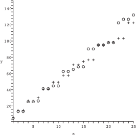
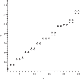
Figure 1: Comparison of the first eigenvalues of the fuzzy Laplacian (circles) with those of the continuum Laplacian (crosses) on the domain of functions with Dirichlet homogeneous boundary conditions. The orders of truncation are $N=10,20,30$.

The fuzzy Laplacian is an automorphism of the algebra on $n\times n$ matrices. In analogy with the fuzzy harmonics described earlier we call the radial part of its eigenoperators Fuzzy Bessel operators. Their symbols, the Fuzzy Bessel functions, form a basis for the fuzzy disc and approximate well the actual Bessel functions, as can be seen from Fig. 2.

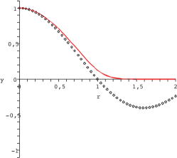
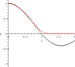
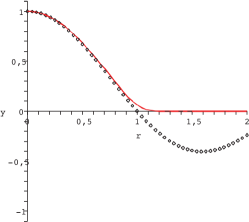
Figure 2: Comparison of the radial shape for the symbol $\Phi^{(N)}_{0,1}(r,\varphi)$ (continuum line), the symbol of the eigenmatrix of the fuzzy Laplacian for $N=10,20,30$, with $\Phi_{0,1}(r,\varphi)$.

Likewise it is possible [44], using the phase operator and phase states known in quantum optics, to have fuzzy angles, i.e. some states concentrated in a small angular region of the disc. Field theories on the fuzzy disc have been studied in [26, 47].

9 Matrix models and the emergence of gravity

Matrix models have a long and distinguished history, especially in string theory [7, 24, 42], in this review we would like to discuss briefly how the discrete basis of the noncommutative products describe earlier gives rise to a matrix model in which gravity is contemplated as an emergent phenomenon, much like the emergent gravity of Sakharov [70]. Here by emergent gravity we really mean the emergence of fields moving in a curved background. This is a more modest goal than having the metric degrees of freedom emerging as quantized fields. This would be tantamount to have a full theory of quantum gravity. And as is known, we are not yet there ….

Since for the kind of products we are considering derivations are inner automorphisms of the algebra since they can be expressed by a commutator:

$$\frac{\partial}{\partial x_{\mu}}f={\mathrm{i}}\theta_{\mu\nu}^{-1}[x^{\nu},f]_{*}.$$ (9.1)

If one considers a U(1) gauge theory on this space, with unitary transformations given by star unitary elements $U*U^{\dagger}=\mathbb{I}$, the action invariant for the transformation $F\to U*F*U^{\dagger}$ is given by

$$S=-\int{\mathrm{d}}x\frac{1}{4}F*F.$$

One can define a covariant derivative

$$D_{\mu}f=\partial_{\mu}f-{\mathrm{i}}[f,A_{\mu}]_{*}={\mathrm{i}}\theta^{-1}_{\mu\nu}[X^{\mu},f]_{*}$$

and

$$F^{\mu\nu}=[D^{\mu},D^{\nu}]_{\star}=[X^{\mu},X^{\nu}]_{\star}+\theta^{\mu\nu}.$$

The connection between commutator with the coordinates and derivatives (9.1), suggest [55] the definition of covariant coordinates

$$X^{\mu}=x^{\mu}+\theta^{\mu\nu}A_{\nu}$$

and consequently

$$D_{\mu}f={\mathrm{i}}\theta^{-1}_{\mu\nu}[X^{\mu},f]_{\star}=\partial_{\mu}f-{\mathrm{i}}[f,A_{\mu}]_{\star}.$$

Therefore we have

$$F^{\mu\nu}=[D^{\mu},D^{\nu}]_{\star}=[X^{\mu},X^{\nu}]_{\star}+\theta^{\mu\nu}.$$

The constant $\theta$ can be reabsorbed by a field redefinition and the action is the square of this quantity, integrated over spacetime.

The action can therefore be rewritten, in the matrix basis as

$$S=-\frac{1}{4g}\operatorname{tr}[X^{\mu},X^{\nu}][X^{\mu^{\prime}},X^{\nu^{\prime}}]g_{\mu\mu^{\prime}}g_{\nu\nu^{\prime}},$$ (9.2)

where the $X$’s are operators (matrices) and the metric $g_{\mu\mu^{\prime}}$ is the flat Minkowski (or Euclidean) metric.

We now briefly remind how gravity emerges from this model [75]. The equations of motion corresponding to the action (9.2):

$$[X^{\mu},[X^{\nu},X^{\mu^{\prime}}]]g_{\mu\mu^{\prime}}=0.$$

These equations have different solutions, which we call vacua. One solution in particular corresponds to the star product generated by (3.10). We call the matrixes correspondding to this particular solution $X_{0}$, hence

$$[X_{0}^{\mu},X_{0}^{\nu}]={\mathrm{i}}\theta^{\mu\nu}.$$ (9.3)

Note that the relation can only be valid if the $X$’s are infinite matrices corresponding to non bounded operators. Fluctuations around the $X_{0}$’s will give a generalized commutation relation

$$[X^{\mu},X^{\nu}]={\mathrm{i}}\theta(X),$$

where we have defined the matrices $X^{\mu}=X_{0}^{\mu}+A^{\mu}$ in analogy with the covariant coordinates.

An important result obtained in [75] (see also [83]) is obtained if one couples the theory to a scaler field $\Sigma$. At this stage the meaning and origin of this field is yet undetermined, it is a field which couples to the noncommutative space time. The free action of this field, using the fact that the derivative are expressed as commutators with the coordinates, is:

$$\operatorname{tr}[X^{\mu},\Sigma][X^{\nu},\Sigma]g_{\mu\nu}\sim\int{\mathrm{d}}x(D_{\mu^{\prime}}\Sigma)(D_{\nu^{\prime}}\Sigma)\theta^{\mu\mu^{\prime}}\theta^{\nu\nu^{\prime}}g_{\mu\nu}=\int{\mathrm{d}}x(D_{\mu}\Sigma)(D_{\nu}\Sigma)G^{\mu\nu}.$$

But it easy to recognize the fact that this is the action of field moving in a non flat background described by the metric

$$G^{\mu\nu}(x)=\theta^{\mu\mu^{\prime}}\theta^{\nu\nu^{\prime}}g_{\mu^{\prime}\nu^{\prime}}.$$

The mere fact that the field was moving in a noncommutative space described by the matrix model has induce a curved background, so that gravity appears as an emergent phenomenon.

The vacuum (9.3) is not the only one. One can consider alternative vacua which have an invariance for some group. For example

$$\bar{X}^{\mu}_{0}=X_{0}^{\mu}\otimes\mathbb{I}_{n}.$$

In this case the theory has an internal space, and a noncommutative ${\rm U}(n)$ symmetry. However the ${\rm U}(1)$ degree of freedom of the theory is the described above, which couple gravitationally. One can separate the trace part $A_{0}$ form the the traceless generators of ${\rm SU}(n)$, considering as fluctuations

$$\bar{X}=\bar{X}_{0}+A_{0}+A_{\alpha}\lambda_{\alpha}.$$

Several models can be constructed based on these matrix models. Extra dimensions can appear in the form of fuzzy spheres [17] and it is possible to have models which start having also characteristics of the standard model [18, 35, 76].

Acknowledgements

We were partially supported by UniNA and Compagnia di San Paolo under the grant “Programma STAR 2013”. F. Lizzi acknowledges support by CUR Generalitat de Catalunya under project FPA2010-20807.

References

• [1] Abe Y., Construction of fuzzy spaces and their applications to matrix models, arXiv:1002.4937.
• [2] Alekseev A.Y., Recknagel A., Schomerus V., Brane dynamics in background fluxes and non-commutative geometry, J. High Energy Phys. 2000 (2000), no. 5, 010, 25 pages, hep-th/0003187.
• [3] Ambjørn J., Makeenko Y.M., Nishimura J., Szabo R.J., Nonperturbative dynamics of noncommutative gauge theory, Phys. Lett. B 480 (2000), 399–408, hep-th/0002158.
• [4] Aschieri P., Dimitrijević M., Kulish P., Lizzi F., Wess J., Noncommutative spacetimes: symmetries in noncommutative geometry and field theory, Lecture Notes in Physics, Vol. 774, Springer-Verlag, Berlin, 2009.
• [5] Balachandran A.P., Kürkçüoǧlu S., Gupta K.S., Edge currents in non-commutative Chern–Simons theory from a new matrix model, J. High Energy Phys. 2003 (2003), no. 9, 007, 17 pages, hep-th/0306255.
• [6] Balachandran A.P., Kürkçüoǧlu S., Vaidya S., Lectures on fuzzy and fuzzy SUSY physics, hep-th/0511114.
• [7] Banks T., Fischler W., Shenker S.H., Susskind L., M theory as a matrix model: a conjecture, Phys. Rev. D 55 (1997), 5112–5128, hep-th/9610043.
• [8] Basu P., Chakraborty B., Scholtz F.G., A unifying perspective on the Moyal and Voros products and their physical meanings, J. Phys. A: Math. Theor. 44 (2011), 285204, 11 pages, arXiv:1101.2495.
• [9] Bayen F., Flato M., Fronsdal C., Lichnerowicz A., Sternheimer D., Deformation theory and quantization. I. Deformations of symplectic structures, Ann. Physics 111 (1978), 61–110.
• [10] Bayen F., Flato M., Fronsdal C., Lichnerowicz A., Sternheimer D., Deformation theory and quantization. II. Physical applications, Ann. Physics 111 (1978), 111–151.
• [11] Beiser S., Römer H., Waldmann S., Convergence of the Wick star product, Comm. Math. Phys. 272 (2007), 25–52, math.QA/0506605.
• [12] Berezin F.A., General concept of quantization, Comm. Math. Phys. 40 (1975), 153–174.
• [13] Blaschke D.N., Grosse H., Schweda M., Non-commutative ${\rm U}(1)$ gauge theory on ${\mathbb{R}}^{4}_{\Theta}$ with oscillator term and BRST symmetry, Europhys. Lett. 79 (2007), 61002, 3 pages, arXiv:0705.4205.
• [14] Blaschke D.N., Hohenegger S., Schweda M., Divergences in non-commutative gauge theories with the Slavnov term, J. High Energy Phys. 2005 (2005), no. 11, 041, 29 pages, arXiv:1302.2903.
• [15] Bratteli O., Inductive limits of finite dimensional $C^{\ast}$-algebras, Trans. Amer. Math. Soc. 171 (1972), 195–234.
• [16] Cahill K.E., Glauber R.J., Ordered expansions in boson amplitude operators, Phys. Rev. 177 (1969), 1857–1881.
• [17] Chatzistavrakidis A., Steinacker H., Zoupanos G., On the fermion spectrum of spontaneously generated fuzzy extra dimensions with fluxes, Fortschr. Phys. 58 (2010), 537–552, arXiv:0909.5559.
• [18] Chatzistavrakidis A., Steinacker H., Zoupanos G., Intersecting branes and a standard model realization in matrix models, J. High Energy Phys. 2011 (2011), no. 9, 115, 36 pages, arXiv:1107.0265.
• [19] Chu C.-S., Madore J., Steinacker H., Scaling limits of the fuzzy sphere at one loop, J. High Energy Phys. 2001 (2001), no. 8, 038, 17 pages, hep-th/0106205.
• [20] Connes A., Noncommutative geometry, Academic Press, Inc., San Diego, CA, 1994.
• [21] D’Andrea F., Lizzi F., Várilly J.C., Metric properties of the fuzzy sphere, Lett. Math. Phys. 103 (2013), 183–205, arXiv:1209.0108.
• [22] de Goursac A., Wallet J.-C., Wulkenhaar R., Noncommutative induced gauge theory, Eur. Phys. J. C 51 (2007), 977–987, hep-th/0703075.
• [23] de Goursac A., Wallet J.-C., Wulkenhaar R., On the vacuum states for noncommutative gauge theory, Eur. Phys. J. C 56 (2008), 293–304, arXiv:0803.3035.
• [24] Dijkgraaf R., Verlinde E., Verlinde H., Matrix string theory, Nuclear Phys. B 500 (1997), 43–61, hep-th/9703030.
• [25] Estrada R., Gracia-Bondía J.M., Várilly J.C., On asymptotic expansions of twisted products, J. Math. Phys. 30 (1989), 2789–2796.
• [26] Falomir H., Franchino Viñas S.A., Pisani P.A.G., Vega F., Boundaries in the Moyal plane, J. High Energy Phys. 2013 (2013), no. 12, 024, 20 pages, arXiv:1307.4464.
• [27] Galluccio S., Lizzi F., Vitale P., Twisted noncommutative field theory with the Wick–Voros and Moyal products, Phys. Rev. D 78 (2008), 085007, 14 pages, arXiv:0810.2095.
• [28] Galluccio S., Lizzi F., Vitale P., Translation invariance, commutation relations and ultraviolet/infrared mixing, J. High Energy Phys. 2009 (2009), no. 9, 054, 18 pages, arXiv:0907.3640.
• [29] Gayral V., Gracia-Bondía J.M., Iochum B., Schücker T., Várilly J.C., Moyal planes are spectral triples, Comm. Math. Phys. 246 (2004), 569–623, hep-th/0307241.
• [30] Géré A., Vitale P., Wallet J.-C., Quantum gauge theories on noncommutative 3-d space, arXiv:1312.6145.
• [31] Géré A., Wallet J.-C., Spectral theorem in noncommutative field theories I: Jacobi dynamics, arXiv:1402.6976.
• [32] Gracia-Bondía J.M., Lizzi F., Marmo G., Vitale P., Infinitely many star products to play with, J. High Energy Phys. 2002 (2002), no. 4, 026, 35 pages, hep-th/0112092.
• [33] Gracia-Bondía J.M., Várilly J.C., Algebras of distributions suitable for phase-space quantum mechanics. I, J. Math. Phys. 29 (1988), 869–879.
• [34] Groenewold H.J., On the principles of elementary quantum mechanics, Physica 12 (1946), 405–460.
• [35] Grosse H., Lizzi F., Steinacker H., Noncommutative gauge theory and symmetry breaking in matrix models, Phys. Rev. D 81 (2010), 085034, 12 pages, arXiv:1001.2703.
• [36] Grosse H., Wulkenhaar R., Renormalisation of $\phi^{4}$-theory on noncommutative ${\mathbb{R}}^{2}$ in the matrix base, J. High Energy Phys. 2003 (2003), no. 12, 019, 26 pages, hep-th/0307017.
• [37] Grosse H., Wulkenhaar R., Renormalisation of $\phi^{4}$-theory on noncommutative ${\mathbb{R}}^{4}$ in the matrix base, Comm. Math. Phys. 256 (2005), 305–374, hep-th/0401128.
• [38] Gurau R., Magnen J., Rivasseau V., Tanasa A., A translation-invariant renormalizable non-commutative scalar model, Comm. Math. Phys. 287 (2009), 275–290, arXiv:0802.0791.
• [39] Hammou A.B., Lagraa M., Sheikh-Jabbari M.M., Coherent state induced star product on ${\mathbb{R}}^{3}_{\lambda}$ and the fuzzy sphere, Phys. Rev. D 66 (2002), 025025, 11 pages, hep-th/0110291.
• [40] Hayakawa M., Perturbative analysis on infrared aspects of noncommutative QED on ${\mathbb{R}}^{4}$, Phys. Lett. B 478 (2000), 394–400, hep-th/9912094.
• [41] Hoppe J., Quantum theory of a massless relativistic surface and a two-dimensional bound state problem, Ph.D. Thesis, Massachusetts Institute of Technology, 1982, reprinted in Soryushiron Kenkyu 80 (1989), 145–202.
• [42] Ishibashi N., Kawai H., Kitazawa Y., Tsuchiya A., A large-$N$ reduced model as superstring, Nuclear Phys. B 498 (1997), 467–491, hep-th/9612115.
• [43] Iso S., Kimura Y., Tanaka K., Wakatsuki K., Noncommutative gauge theory on fuzzy sphere from matrix model, Nuclear Phys. B 604 (2001), 121–147, hep-th/0101102.
• [44] Kobayashi S., Asakawa T., Angles in fuzzy disc and angular noncommutative solitons, J. High Energy Phys. 2013 (2013), no. 4, 145, 22 pages, arXiv:1206.6602.
• [45] Koekoek R., Lesky P.A., Swarttouw R.F., Hypergeometric orthogonal polynomials and their $q$-analogues, Springer Monographs in Mathematics, Springer-Verlag, Berlin, 2010.
• [46] Landi G., Lizzi F., Szabo R.J., From large $N$ matrices to the noncommutative torus, Comm. Math. Phys. 217 (2001), 181–201, hep-th/9912130.
• [47] Lizzi F., Spisso B., Noncommutative field theory: numerical analysis with the fuzzy disk, Internat. J. Modern Phys. A 27 (2012), 1250137, 26 pages, arXiv:1207.4998.
• [48] Lizzi F., Vitale P., Zampini A., From the fuzzy disc to edge currents in Chern–Simons theory, Modern Phys. Lett. A 18 (2003), 2381–2387, hep-th/0309128.
• [49] Lizzi F., Vitale P., Zampini A., The fuzzy disc, J. High Energy Phys. 2003 (2003), no. 8, 057, 16 pages, hep-th/0306247.
• [50] Lizzi F., Vitale P., Zampini A., The beat of a fuzzy drum: fuzzy Bessel functions for the disc, J. High Energy Phys. 2005 (2005), no. 9, 080, 32 pages, hep-th/0506008.
• [51] Lizzi F., Vitale P., Zampini A., The fuzzy disc: a review, J. Phys. Conf. Ser. 53 (2006), 830–842.
• [52] Lizzi F., Zampini A., Szabo R.J., Geometry of the gauge algebra in non-commutative Yang–Mills theory, J. High Energy Phys. 2001 (2001), no. 8, 032, 54 pages, hep-th/0107115.
• [53] Madore J., The fuzzy sphere, Classical Quantum Gravity 9 (1992), 69–87.
• [54] Madore J., An introduction to noncommutative differential geometry and its physical applications, London Mathematical Society Lecture Note Series, Vol. 257, 2nd ed., Cambridge University Press, Cambridge, 1999.
• [55] Madore J., Schraml S., Schupp P., Wess J., Gauge theory on noncommutative spaces, Eur. Phys. J. C 16 (2000), 161–167, hep-th/0001203.
• [56] Man’ko O.V., Man’ko V.I., Marmo G., Alternative commutation relations, star products and tomography, J. Phys. A: Math. Gen. 35 (2002), 699–719, quant-ph/0112110.
• [57] Man’ko V.I., Marmo G., Vitale P., Phase space distributions and a duality symmetry for star products, Phys. Lett. A 334 (2005), 1–11, hep-th/0407131.
• [58] Man’ko V.I., Marmo G., Vitale P., Zaccaria F., A generalization of the Jordan–Schwinger map: the classical version and its $q$ deformation, Internat. J. Modern Phys. A 9 (1994), 5541–5561, hep-th/9310053.
• [59] Martinetti P., Vitale P., Wallet J.-C., Noncommutative gauge theories on ${\mathbb{R}}_{\theta}^{2}$ as matrix models, J. High Energy Phys. 2013 (2013), no. 9, 051, 26 pages, arXiv:1303.7185.
• [60] Matusis A., Susskind L., Toumbas N., The IR/UV connection in non-commutative gauge theories, J. High Energy Phys. 2000 (2000), no. 12, 002, 18 pages, hep-th/0002075.
• [61] Minwalla S., Van Raamsdonk M., Seiberg N., Noncommutative perturbative dynamics, J. High Energy Phys. 2000 (2000), no. 2, 020, 31 pages, hep-th/9912072.
• [62] Moyal J.E., Quantum mechanics as a statistical theory, Proc. Cambridge Philos. Soc. 45 (1949), 99–124.
• [63] Panero M., Numerical simulations of a non-commutative theory: the scalar model on the fuzzy sphere, J. High Energy Phys. 2007 (2007), no. 5, 082, 20 pages, hep-th/0608202.
• [64] Perelomov A., Generalized coherent states and their applications, Texts and Monographs in Physics, Springer-Verlag, Berlin, 1986.
• [65] Pimsner M., Voiculescu D., Imbedding the irrational rotation $C^{\ast}$-algebra into an AF-algebra, J. Operator Theory 4 (1980), 201–210.
• [66] Pinzul A., Stern A., Edge states from defects on the noncommutative plane, Modern Phys. Lett. A 18 (2003), 2509–2516, hep-th/0307234.
• [67] Rieffel M.A., $C^{\ast}$-algebras associated with irrational rotations, Pacific J. Math. 93 (1981), 415–429.
• [68] Rieffel M.A., Matrix algebras converge to the sphere for quantum Gromov–Hausdorff distance, Mem. Amer. Math. Soc. 168 (2004), 67–91, math.OA/0108005.
• [69] Rosa L., Vitale P., On the $\star$-product quantization and the Duflo map in three dimensions, Modern Phys. Lett. A 27 (2012), 1250207, 15 pages, arXiv:1209.2941.
• [70] Sakharov A.D., Vacuum quantum fluctuations in curved space and the theory of gravitation, Sov. Phys. Dokl. 12 (1968), 1040–1041, reprinted in Gen. Relativity Gravitation 32 (2000), 365–367.
• [71] Scholtz F.G., Chakraborty B., Govaerts J., Vaidya S., Spectrum of the non-commutative spherical well, J. Phys. A: Math. Theor. 40 (2007), 14581–14592, arXiv:0709.3357.
• [72] Seiberg N., Witten E., String theory and noncommutative geometry, J. High Energy Phys. 1999 (1999), no. 9, 032, 93 pages, hep-th/9908142.
• [73] Soloviev M.A., Algebras with convergent star products and their representations in Hilbert spaces, J. Math. Phys. 54 (2013), 073517, 16 pages, arXiv:1312.6571.
• [74] Spisso B., Wulkenhaar R., A numerical approach to harmonic noncommutative spectral field theory, Internat. J. Modern Phys. A 27 (2012), 1250075, 25 pages, arXiv:1111.3050.
• [75] Steinacker H., Emergent gravity from noncommutative gauge theory, J. High Energy Phys. 2007 (2007), no. 12, 049, 36 pages, arXiv:0708.2426.
• [76] Steinacker H., Zahn J., An extended standard model and its Higgs geometry from the matrix model, arXiv:1401.2020.
• [77] Szabo R.J., Quantum field theory on noncommutative spaces, Phys. Rep. 378 (2003), 207–299, hep-th/0109162.
• [78] Tanasa A., Vitale P., Curing the UV/IR mixing for field theories with translation-invariant star products, Phys. Rev. D 81 (2010), 065008, 12 pages, arXiv:0912.0200.
• [79] Várilly J.C., Gracia-Bondía J.M., Algebras of distributions suitable for phase-space quantum mechanics. II. Topologies on the Moyal algebra, J. Math. Phys. 29 (1988), 880–887.
• [80] Varshalovich D.A., Moskalev A.N., Khersonskiĭ V.K., Quantum theory of angular momentum, World Scientific Publishing Co., Inc., Teaneck, NJ, 1988.
• [81] Varshovi A.A., Groenewold–Moyal product, $\alpha^{\star}$-cohomology, and classification of translation-invariant non-commutative structures, J. Math. Phys. 54 (2013), 072301, 9 pages, arXiv:1210.1004.
• [82] Vitale P., Wallet J.-C., Noncommutative field theories on ${\mathbb{R}}^{3}_{\lambda}$: towards UV/IR mixing freedom, J. High Energy Phys. 2013 (2013), no. 4, 115, 36 pages, arXiv:1212.5131.
• [83] Yang H.S., Emergent gravity from noncommutative space-time, Internat. J. Modern Phys. A 24 (2009), 4473–4517, hep-th/0611174.
\LastPageEnding