Larson’s scaling laws, and the gravitational instability of clumpy discs at high redshift

Abstract

Gravitational instabilities play a primary role in shaping the clumpy structure and powering the star formation activity of gas-rich high-redshift galaxies. Here we analyse the stability of such systems, focusing on the size and mass ranges of unstable regions in the disc. Our analysis takes into account the mass-size and linewidth-size scaling relations observed in molecular gas, originally discovered by Larson. We show that such relations can have a strong impact on the size and mass of star-forming clumps, as well as on the stability properties of the disc at all observable scales, making the classical Toomre parameter a highly unreliable indicator of gravitational instability. For instance, a disc with $Q=1$ can be far from marginal instability, while a disc with $Q\ll 1$ can be marginally unstable. Our work raises an important caveat: if clumpy discs at high redshift have scale-dependent surface densities and velocity dispersions, as implied by the observed clump scaling relations, then we cannot thoroughly understand their stability and star formation properties unless we perform multi-scale observations. This will soon be possible thanks to dedicated ALMA surveys, which will explore the physical properties of super-giant molecular clouds at the peak of cosmic star formation and beyond.

1 INTRODUCTION

Today it is well established that the majority of the stellar mass observed in galaxies formed at high redshift, and in particular that the mean cosmological star-formation-rate density peaks at redshift 1–3 (e.g., Hopkins & Beacom 2006). Recent semi-empirical studies (e.g., Behroozi et al. 2013) have allowed understanding how the peak redshift of individual galaxies depends, on average, on the mass of the host dark matter halo, with today’s $L_{*}$ galaxy population forming stars at peak efficiency around $z=1\mbox{--}2$. Understanding the complex behaviour of galaxy assembly is a daunting task for galaxy formation theory (e.g., Weinmann et al. 2011), and highlights the need to build robust models that are capable of predicting how star formation proceeds in high-redshift galaxies.

The morphology and star formation properties of massive high-redshift galaxies are very different from those of present-day quiescent spirals and ellipticals. Extended clumpy irregular discs with kpc-sized star-forming clumps as massive as $M\sim 10^{7}\mbox{--}10^{9}\,\mbox{M}_{\odot}$ are observed in the Hubble Ultra Deep Field (UDF; e.g., Elmegreen et al. 2007, 2009), a population that is rare today. Multi-wavelength observational evidence (e.g., Elmegreen & Elmegreen 2006; Shapiro et al. 2008; Tacconi et al. 2010) suggests that clumps generally form in gas-rich spiral discs rather than in mergers, although the latter scenario cannot be completely ruled out (e.g., Overzier et al. 2008). Numerical work by Bournaud et al. (2007) and Elmegreen et al. (2008) demonstrated that internal disc fragmentation can reproduce many of the observables of clumpy high-redshift galaxies. Using high-resolution hydrodynamical simulations in a fully cosmological framework, Agertz et al. (2009b) demonstrated that super-massive clumps are a natural outcome of fragmenting massive gas-rich discs, formed from multi-phase cosmological accretion (see also Ceverino et al. 2010).

The size and mass of such clumps can be predicted using simple arguments, if one assumes that the disc is marginally unstable according to Toomre’s stability criterion (e.g., Noguchi 1998, 1999; Dekel et al. 2009; Genzel et al. 2011). This assumption makes sense because current dynamical models of high-redshift star-forming galaxies suggest that their discs are driven by self-regulation processes, which keep them close to marginal instability (e.g., Noguchi 1998, 1999; Agertz et al. 2009a; Dekel et al. 2009; Burkert et al. 2010; Krumholz & Burkert 2010; Cacciato et al. 2012; Forbes et al. 2012, 2014). If $Q\equiv\kappa\sigma/\pi G\Sigma=1$, then there is a single unstable wavelength, $\lambda=2\sigma^{2}/G\Sigma$, and the associated mass is $M\sim\Sigma\lambda^{2}=4\sigma^{4}/G^{2}\Sigma$. In the gas disc of the Milky Way, these quantities are comparable to the maximum size and mass of giant molecular clouds, i.e. $\lambda\sim 100\,\mbox{pc}$ and $M\sim 10^{6}\,\mbox{M}_{\odot}$ (see, e.g., Glazebrook 2013). In high-redshift discs, both the surface density $\Sigma$ and the velocity dispersion $\sigma$ of molecular gas are typically one order of magnitude larger than in the Milky Way (see again Glazebrook 2013). As $\lambda\propto\sigma^{2}/\Sigma$ and $M\propto\sigma^{4}/\Sigma$, we get $\lambda\sim 1\,\mbox{kpc}$ and $M\sim 10^{9}\,\mbox{M}_{\odot}$, which are the typical clump size and mass. Genzel et al. (2011) and Wisnioski et al. (2012) showed that the clumps are located in regions of the disc where $Q\la 1$. This provides further evidence that in clumpy discs at high redshift there is a strong link between star formation and gravitational instability.

In spite of its predictive power, such a scenario neglects an important aspect of the problem: in clumpy discs, the surface density and velocity dispersion depend on the size of the region over which they are measured (Romeo et al. 2010; Hoffmann & Romeo 2012), contrary to what is generally assumed (see, e.g., Glazebrook 2013). In fact, there is mounting evidence that molecular gas is characterized by mass-size and linewidth-size scaling relations:

$$\Sigma\propto\ell^{a},\;\;\;\;\;\mathrm{i.e.}\ M\propto\ell^{2+a},$$ (1)

$$\sigma\propto\ell^{b},$$ (2)

where $\Sigma$ and $M$ are the mass column density and the mass of the clump, $\sigma$ is its 1D velocity dispersion, and $\ell$ is the clump size.

1. The most compelling evidence of such a link comes from observations of molecular clouds in the Milky Way and nearby galaxies (see, e.g., Hennebelle & Falgarone 2012, and references therein; Donovan Meyer et al. 2013; Kauffmann et al. 2013; Kritsuk et al. 2013; Kruijssen & Longmore 2013). These observations show that both Galactic and extragalactic molecular clouds are fairly well described by the so-called ‘Larson’s scaling laws’, $a=0$ and $b=\frac{1}{2}$ (Larson 1981; Solomon et al. 1987), although the uncertainties are still significant: $-0.8\la a\la 0.7$ (Beaumont et al. 2012), and $0.2\la b\la 1.1$ (Shetty et al. 2012).

2. Similar scaling exponents are found in high-resolution simulations of molecular clouds and supersonic turbulence (see, e.g., Hennebelle & Falgarone 2012, and references therein; Beaumont et al. 2013; Federrath 2013; Kritsuk et al. 2013; Bertram et al. 2014; Fujimoto et al. 2014; Ward et al. 2014). The latter simulations show that $a$ depends not only on the Mach number of the gas, but also on turbulence forcing (Federrath et al. 2009, 2010; Federrath 2013) and self-gravity (Collins et al. 2012; Kritsuk et al. 2013). In contrast, at high Mach numbers, $b$ is approximately constant and close to 0.5 (see again Federrath 2013; Kritsuk et al. 2013).

3. Larson-type scaling relations have recently been observed, for the first time, in the dense star-forming clumps of a high-redshift galaxy: the strongly lensed sub-millimetre galaxy SMM J2135–0102 at $z=2.32$, also known as the cosmic eyelash (Swinbank et al. 2011). Although this is the only detection of super-giant molecular clouds at high redshift, it will soon be followed by many such observations, which will exploit the unprecedented resolution and sensitivity of the Atacama Large Millimeter/submillimeter Array (ALMA) for exploring the physical properties of molecular gas at $z\ga 2$ (see, e.g., Glazebrook 2013).

Romeo et al. (2010) explored the gravitational instability of clumpy gas discs, and showed that the mass-size and linewidth-size scaling relations of the clumps can have a strong impact on disc instability. For instance, they can excite three main instability regimes, two of which have no classical counterpart. Hoffmann & Romeo (2012) generalized this result to two-component discs of clumpy gas and old stars, and analysed the stability of spirals from The H i Nearby Galaxy Survey (THINGS).

In this paper, we investigate the gravitational instability of clumpy discs at high redshift, focusing on the size and mass ranges of unstable regions (see Sect. 2). We begin by spelling out the assumptions of our stability analysis and summarizing the results of Romeo et al. (2010), which are fundamental to a proper understanding of this paper (see Sect. 2.1). Next, we discuss the effects of varying the clump scaling relations across the observed ranges of $a$ and $b$, and illustrate how the spatial resolution affects the inferred stability properties of the disc, if the observed $\Sigma$ and $\sigma$ are scale-dependent (see Sect. 2.2). This is a complex aspect of the problem, which should be taken into account when analysing the stability of high-redshift star-forming galaxies. Last but not least, we discuss the properties of discs close to marginal instability (see Sect. 2.3). As pointed out above, this is the condition generally assumed for estimating the typical size and mass of the clumps. The disc scale height is expected to play a significant role in this scenario, since it is the scale at which galactic turbulence undergoes a transition from 3D to 2D (e.g., Bournaud et al. 2010), and this may be accompanied by a break in the clump scaling relations. We discuss this aspect of the problem in Sect. 3. The conclusions of our paper are drawn in Sect. 4.

2 GRAVITATIONAL INSTABILITIES IN CLUMPY DISCS

2.1 The main instability regimes

When analysing the stability of high-redshift star-forming galaxies, it is generally assumed that the surface density of the disc is dominated by molecular gas (g) and young stars ($\star$),

$$\Sigma=\Sigma_{\mathrm{g}}+\Sigma_{\star}\,,$$ (3)

and that the gaseous and stellar components have similar kinematic properties, so that the velocity dispersion of the disc is simply

$$\sigma=\sigma_{\mathrm{g}}=\sigma_{\star}$$ (4)

(e.g., Burkert et al. 2010; Krumholz & Burkert 2010; Puech 2010; Genzel et al. 2014). This assumption makes sense because the mass fraction of molecular gas increases steeply with redshift (e.g., Daddi et al. 2010; Tacconi et al. 2010; Carilli & Walter 2013), and because most of the stars in high-redshift discs were probably formed during the on-going starburst and did not have time to heat up significantly (see again Burkert et al. 2010; Krumholz & Burkert 2010; Puech 2010; Genzel et al. 2014). Older generations of stars with $\sigma_{\mathrm{old}\,\star}\gg\sigma_{\mathrm{g}}$ could also exist (Glazebrook 2013), but they would play a negligible role in the gravitational instability of the disc, even if $\Sigma_{\mathrm{old}\,\star}\ga\Sigma_{\mathrm{g}}$, because the resulting $Q$ stability parameter would still be dominated by the young gaseous-stellar component (Romeo & Falstad 2013).

As pointed out in Sect. 1, this simple model does not capture an important aspect of the problem: in clumpy discs, the mass-size and linewidth-size scaling relations of the clumps can have a strong impact on disc instability (Romeo et al. 2010). Here we take such relations into account, and assume that molecular gas and young stars have similar scaling properties, so that the surface density and the velocity dispersion of the disc are scale-dependent and given by:

$$\Sigma(\ell)=\Sigma_{0}\left(\frac{\ell}{\ell_{0}}\right)^{a},\;\;\;\;\;a=a_{\mathrm{g}}=a_{\star}\,;$$ (5)

$$\sigma(\ell)=\sigma_{0}\left(\frac{\ell}{\ell_{0}}\right)^{b},\;\;\;\;\;b=b_{\mathrm{g}}=b_{\star}\,.$$ (6)

This assumption makes sense because newborn stars inherit the scaling properties of the parent gas (e.g., Larson 1979; Sánchez et al. 2010). Note that, since Eqs (5) and (6) are power laws, the choice of $\ell_{0}$ is arbitrary. What really matters is not $\ell_{0}$ itself but the values of $A\equiv\Sigma_{0}/\ell_{0}^{a}$ and $B\equiv\sigma_{0}/\ell_{0}^{b}$, which unfortunately are poorly constrained. A physically meaningful choice would be to identify $\ell_{0}$ with the disc scale height, $h$, which is the natural smoothing scale of galactic discs (Romeo 1994). However, $\Sigma$ and $\sigma$ are often measured at scales comparable to the disc scale length, $R_{\mathrm{d}}$ (e.g., Puech 2010), or at intermediate scales (e.g., Genzel et al. 2014). To make our analysis readily applicable, we choose to identify $\ell_{0}$ with the scale at which $\Sigma$ and $\sigma$ are measured, and assume that this is also the scale at which the Toomre parameter and the 2D Jeans length are inferred:

$$Q_{0}=\frac{\kappa\sigma_{0}}{\pi G\Sigma_{0}}\,,$$ (7)

$$L_{\mathrm{J}0}\equiv\frac{2\pi}{k_{\mathrm{J}0}}=\frac{\sigma_{0}^{2}}{G\Sigma_{0}}\,,$$ (8)

where $k_{\mathrm{J}0}$ is the 2D Jeans wavenumber (once again, choosing $\ell_{0}=h$ or $\ell_{0}=R_{\mathrm{d}}$ is only conceptually different from our choice; the results are identical). Hereafter we will refer to $\ell_{0}$ as ‘the spatial resolution (scale)’, like Leroy et al. (2008) and Genzel et al. (2014). This scale should not be confused with the resolution limit of the observations: $\Sigma$ and $\sigma$ are usually measured averaging over scales larger than the beam size. Note also that $\ell_{0}$ cannot have any influence on the actual stability properties of the disc. However, since $\ell_{0}$ affects the inferred values of $Q$ and $L_{\mathrm{J}}$, $Q(\ell)=Q_{0}\,(\ell/\ell_{0})^{b-a}$ and $L_{\mathrm{J}}(\ell)=L_{\mathrm{J}0}\,(\ell/\ell_{0})^{2b-a}$, it will also have a significant effect on the derived conditions for gravitational instability.

As discussed above, clumpy discs at high redshift are dynamically similar to gas discs with scale-dependent surface density and velocity dispersion. The gravitational instability of such discs was explored by Romeo et al. (2010). Below we summarize some of their results, which are fundamental to a proper understanding of Sects 2.2 and 2.3.

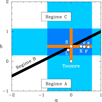
Figure 1: The main instability regimes of clumpy discs. The clumps are characterized by Larson-type scaling relations: $\Sigma\propto\ell^{a}$ and $\sigma\propto\ell^{b}$, where $\Sigma$ is the mass column density, $\sigma$ is the 1D velocity dispersion, and $\ell$ is the clump size. Regime B is a transition between Toomre-like instability (Regime A) and small-scale instability (Regime C). Also shown are the ranges of $a$ and $b$ observed in molecular clouds (shaded), the ranges analysed in Sects 2.2 and 2.3 (highlighted), and the specific values of $(a,b)$ further analysed in Sect. 2.3.

If the disc is subject to local axisymmetric perturbations, as is generally assumed, then its response is described by a dispersion relation that we now write as:

$$\frac{\omega^{2}}{\kappa^{2}}=1-\frac{4}{Q_{0}^{2}}\,\frac{\Sigma(\ell)/\Sigma_{0}}{(\ell/L_{\mathrm{J}0})}+\frac{4}{Q_{0}^{2}}\,\frac{\sigma^{2}(\ell)/\sigma_{0}^{2}}{(\ell/L_{\mathrm{J}0})^{2}}\,,$$ (9)

where $\omega$ and $k=2\pi/\ell$ are the frequency and the wavenumber of the perturbation, and $\kappa$ is the epicyclic frequency. Note that Eq. (9) applies to realistically thick discs (see sect. 2.1 of Romeo et al. 2010). If the disc has volume density $\rho$ and scale height $h$, then $\Sigma\approx 2\rho\ell$ for $\ell\la h$ and $\Sigma\approx 2\rho h$ for $\ell\ga h$. In both cases, the associated mass is $M\sim\Sigma\ell^{2}$. The range $\ell\la h$ corresponds to the case of 3D turbulence (i.e. to the usual clump scaling relations), whereas the range $\ell\ga h$ corresponds to the case of 2D turbulence (i.e. to a large-scale extrapolation of the clump scaling relations; a more realistic case will be discussed in Sect. 3). Note also that Eq. (9) is a relation between $\omega^{2}/\kappa^{2}$ and $\ell/L_{\mathrm{J}0}$, which is affected by four parameters: $Q_{0}$ (the classical stability parameter), $\ell_{0}/L_{\mathrm{J}0}$ (a parameter that couples gravitational instability with spatial resolution), $a$ and $b$ (the logarithmic slopes of the clump scaling relations). It turns out that $a$ and $b$ have an important effect on the shape of the dispersion relation, and hence on the condition for gravitational instability ($\omega^{2}<0$). Variations in the scaling properties of the clumps can drive high-redshift discs across three main instability regimes. Such regimes are illustrated in Fig. 1, together with the ranges of $a$ and $b$ observed in molecular clouds (shaded), and other useful information (which will be discussed in Sects 2.2 and 2.3).

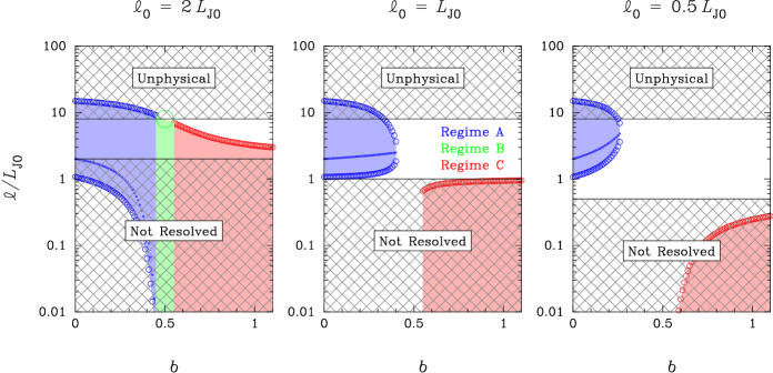
Figure 2: Size range of unstable regions in clumpy discs: effect of varying the linewidth-size scaling relation of the clumps ($\sigma\propto\ell^{b}$) at different spatial resolutions ($\ell_{0}$). We assume that the mass-size scaling relation is $M\propto\ell^{2}$ (Larson’s third law), and that the Toomre parameter (at scale $\ell=\ell_{0}$) is $Q_{0}\equiv\kappa\sigma_{0}/\pi G\Sigma_{0}=0.5$. Lengths are measured in units of the 2D Jeans length, $L_{\mathrm{J}0}\equiv\sigma_{0}^{2}/G\Sigma_{0}$. Also shown is the most unstable scale for discs in Regime A (this quantity vanishes in Regimes B and C).

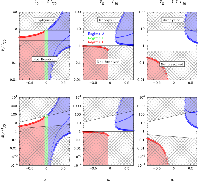
Figure 3: Size range (top) and mass range (bottom) of unstable regions in clumpy discs: effect of varying the mass-size scaling relation of the clumps ($M\propto\ell^{2+a}$) at different spatial resolutions ($\ell_{0}$). We assume that the linewidth-size scaling relation is $\sigma\propto\ell^{1/2}$ (Larson’s first law), and that the Toomre parameter (at scale $\ell=\ell_{0}$) is $Q_{0}\equiv\kappa\sigma_{0}/\pi G\Sigma_{0}=0.5$. Lengths and masses are measured in units of the 2D Jeans length, $L_{\mathrm{J}0}\equiv\sigma_{0}^{2}/G\Sigma_{0}$, and the associated mass, $M_{\mathrm{J}0}\equiv\Sigma(L_{\mathrm{J}0})\,L_{\mathrm{J}0}^{2}$. Also shown are the most unstable scale and the associated mass for discs in Regime A (these quantities vanish in Regimes B and C).

• In Regime A, i.e. for $b<\frac{1}{2}\,(1+a)$ and $-2<a<1$, the stability of the disc is controlled by $Q_{0}$: the disc is stable at all scales if and only if $Q_{0}\geq\overline{Q}_{0}$, where the stability threshold $\overline{Q}_{0}$ depends on $a$, $b$ and $\ell_{0}/L_{\mathrm{J}0}$.

• In Regime C, i.e. for $b>\frac{1}{2}\,(1+a)$ and $-2<a<1$, the stability of the disc is no longer controlled by $Q_{0}$: the disc is always unstable at small scales (i.e. as $\ell/L_{\mathrm{J}0}\rightarrow 0$) and stable at large scales (i.e. as $\ell/L_{\mathrm{J}0}\rightarrow\infty$).

• In Regime B, i.e. for $b=\frac{1}{2}\,(1+a)$ and $-2<a<1$, the disc is stable at all scales if and only if $\ell_{0}/L_{\mathrm{J}0}\leq 1$. This is a regime of transition between stability à la Toomre (Regime A) and instability at small scales (Regime C). Thus even small variations in the scaling properties of the clumps can drive the disc into Regime A or Regime C, and have a strong impact on its gravitational instability.

Note that the stability criteria for Regimes A and B are scale-invariant, i.e. they only apparently depend on the spatial resolution scale $\ell_{0}$: if the disc is stable at a given $\ell_{0}$, then it will also be stable at any other spatial resolution. Note also that similar instability regimes are found in the Milky Way and nearby galaxies, but at scales smaller than about 100 pc (Hoffmann & Romeo 2012).

2.2 Size and mass ranges of unstable regions

Eq. (9) can be used not only for identifying the main instability regimes of clumpy discs, but also for predicting the size and mass ranges of unstable regions in such systems. These correspond to the range(s) of $\ell$ where $\omega^{2}<0$ and to the associated range(s) of $M\equiv\Sigma(\ell)\,\ell^{2}\propto\ell^{2+a}$ (numerical factors are irrelevant, since we are interested in mass ratios). Here we focus on this aspect of the problem, and analyse the effects of varying the clump scaling relations across the ranges highlighted in Fig. 1. The idea behind our choices of $a$ and $b$ is to vary one parameter at a time, starting from $a=0$ and $b=\frac{1}{2}$ (Larson’s scaling laws), and spanning the ranges of $a$ and $b$ observed in molecular clouds (shaded). We vary $b$ down to $b=0$ so as to include the classical case of Toomre instability. Concerning the other parameters, we choose $\ell_{0}/L_{\mathrm{J}0}=0.5,1,2$ so as to sample the (in)stability condition for discs governed by Larson’s scaling laws (Regime B), and $Q_{0}=0.5$ so as to represent the state of violent gravitational instability observed in high-redshift star-forming galaxies (e.g., Puech 2010; Genzel et al. 2014). Note that these values of $\ell_{0}/L_{\mathrm{J}0}$ and $Q_{0}$ match those found in the rings and outer discs of SINS/zC-SINF galaxies at $z\sim 2$ (Genzel et al. 2014).

Before discussing the results of our analysis, let us make a final remark about our parameter choice. By fixing $Q_{0}$ while changing $\ell_{0}/L_{\mathrm{J}0}$, we are also implicitly changing $\Sigma_{0}$ and $\sigma_{0}$, albeit not according to a unique set of scaling relations (otherwise $Q_{0}$ would also change). Doing so, we are probing different physical states or regions of the disc. Our parameter choice is meant to illustrate a few interesting examples of disc stability properties relevant to high-redshift star-forming galaxies, as we discuss below.

2.2.1 Effect of varying the linewidth-size scaling relation of the clumps

Let us first discuss the effect of varying $b$, which is illustrated in Fig. 2. We only show the size range of unstable regions (shaded), since the associated mass range follows trivially from Larson’s third law ($M\propto\ell^{2}$; remember that here $a=0$). For $b=0$, the classical case of Toomre instability, the range of unstable scales can be easily computed since $\omega^{2}(\ell)<0$ is a quadratic inequality. The largest and the smallest (marginally) unstable scales are then $\ell=(8\pm 4\sqrt{3}\,)L_{\mathrm{J}0}\approx 15L_{\mathrm{J}0}\mbox{ and }L_{\mathrm{J}0}$. Within this range, there is a scale that corresponds to the fastest growing mode, and therefore plays a primary role in the classical instability scenario. This is ‘the most unstable scale’, which can be computed by minimizing $\omega^{2}(\ell)$: $\ell=2L_{\mathrm{J}0}\ (=2\sigma_{0}^{2}/G\Sigma_{0})$. For all other values of $b$, the three scales introduced above depend on the coupling between gravitational instability and spatial resolution.

When the 2D Jeans length is not resolved, the disc is unstable over a broad range of $\ell$ for all values of $b$ (see the left panel of Fig. 2). The largest unstable scale decreases gradually with increasing $b$, while the smallest and the most unstable scales decrease steeply as $b$ approaches 0.5 (Regime A) and vanish thereafter (Regimes B and C). Note, however, that scales $\ell\la 2L_{\mathrm{J}0}$ cannot be resolved, and scales $\ell\ga 8L_{\mathrm{J}0}$ are unphysical because they exceed the typical size of galaxies at $z\sim 2$. This implies (i) that the observable size range of unstable regions is constant up to $b\approx 0.5$, and shrinks by a factor of 6 from $b\approx 0.5$ to $b=1.1$; and (ii) that none of the ‘characteristic’ unstable scales plays a significant role in Toomre-like instabilities, when $\ell_{0}=2L_{\mathrm{J}0}$ and $Q_{0}=0.5$.

When the 2D Jeans length is resolved, the disc is no longer unstable for all values of $b$ (see now the middle and right panels of Fig. 2). There are two distinct instability domains, but only one of them is observable: the domain of Toomre-like instabilities (Regime A). The higher the spatial resolution, the smaller this domain. Note that there is a value of $b<0.5$ for which the disc is marginally unstable, like a classical disc with $Q_{0}=1$. In such a case, the instability range collapses into a single characteristic scale, which is of the order of the typical size of the clumps (e.g., Noguchi 1998, 1999; Dekel et al. 2009; Genzel et al. 2011). When $\ell_{0}=L_{\mathrm{J}0}$, marginal instability occurs for $b\approx 0.4$ and the characteristic instability scale is about $2.5L_{\mathrm{J}0}$, i.e. 25% larger than in the classical case ($2L_{\mathrm{J}0}$). When $\ell_{0}=0.5L_{\mathrm{J}0}$, the disc is marginally unstable for $b\approx 0.25$ and the characteristic scale is about $5L_{\mathrm{J}0}$, which is comparable to the half-light radius of the galaxy.

2.2.2 Effect of varying the mass-size scaling relation of the clumps

The effect of varying $a$ is illustrated in Fig. 3. A comparison between the top panels of this figure and Fig. 2 shows that increasing $a$ has a qualitatively similar effect to decreasing $b$. This is basically because, as $a$ varies from $-$0.8 to 0.7, the disc spans all the main instability regimes, starting from Regime C and ending with Regime A. Despite this similarity, $a$ has a stronger impact on disc instability than $b$. For example, when $\ell_{0}=L_{\mathrm{J}0}$, the characteristic instability scale for a marginally unstable disc ($a\approx 0.15$) is about $3L_{\mathrm{J}0}$, i.e. 50% larger than in the classical case. And, when $\ell_{0}=0.5L_{\mathrm{J}0}$, such a scale exceeds the typical size of galaxies at $z\sim 2$. The bottom panels of Fig. 3 show that $a$ has an even stronger impact on the mass range of unstable regions. This is because $M=M_{\mathrm{J}0}\,(\ell/L_{\mathrm{J}0})^{2+a}$ with $2+a>1$, and because variations in $M$ are now boosted by the $a$-dependent factor $(\ell/L_{\mathrm{J}0})^{a}$. Note also that the 2D Jeans mass is defined consistent with the mass-size scaling relation, $M_{\mathrm{J}0}\equiv\Sigma(L_{\mathrm{J}0})\,L_{\mathrm{J}0}^{2}$, and so are all other relevant masses. Hence the lower and upper bounds of the observable range are themselves functions of $a$ for a given $M_{\mathrm{J}0}$, as is shown in the bottom panels of Fig. 3.

2.3 Discs close to marginal instability

Current dynamical models of high-redshift star-forming galaxies suggest that their discs are driven by self-regulation processes, which keep them close to marginal instability (e.g., Noguchi 1998, 1999; Agertz et al. 2009a; Dekel et al. 2009; Burkert et al. 2010; Krumholz & Burkert 2010; Cacciato et al. 2012; Forbes et al. 2012, 2014). In Sect. 2.2, we have shown that clumpy discs can be marginally unstable even if $Q_{0}\ll 1$. Here we analyse the case $Q_{0}=1$, which is classically associated with marginal instability. Note that this value of $Q_{0}$ is close to the median value $Q_{0}\approx 0.9$ found in the inner discs of SINS/zC-SINF galaxies at $z\sim 2$, as we infer from table 1 of Genzel et al. (2014). Note also that the median value of the 2D Jeans length in such discs is $L_{\mathrm{J}0}\approx 0.4\;\mbox{kpc}$, and that the spatial resolution scale is $\ell_{0}\approx 2\;\mbox{kpc}$, hence $\ell_{0}/L_{\mathrm{J}0}\approx 5$. This means that the 2D Jeans length is far from being resolved, and so are the size and mass ranges of unstable regions for all observed values of $a$ and $b$. This is consistent with the gravitational quenching found by Genzel et al. (2014), but it also means that we need much higher resolution to probe gravitational instabilities in such discs.

What would we observe if the 2D Jeans length were marginally resolved ($\ell_{0}=L_{\mathrm{J}0}$) and the Toomre parameter were still unity? As $a$ and $b$ span the ranges analysed in Sect. 2.2, we would observe two instability domains: the classical domain of marginally unstable discs ($a=b=0$, $\ell=2L_{\mathrm{J}0}$, $M=4M_{\mathrm{J}0}$), and a domain of Toomre-like instabilities ($0.5\leq a\leq 0.7$, $b=\frac{1}{2}$). In such a case, the disc is marginally unstable for $a=b=\frac{1}{2}$, the characteristic instability scale is $\ell\approx 4L_{\mathrm{J}0}$, and the associated mass is $M\approx 30M_{\mathrm{J}0}$. This is consistent with the results of Romeo et al. (2010), who found that the stability criterion for Regime A degenerates into Toomre’s stability criterion for all $a=b$. As $Q_{0}=1$ is a case of special interest, let us also analyse specific values of $(a,b)$: the cases illustrated in Fig. 1.

• Case L, i.e. $(a,b)=(-0.1,0.38)$, represents the original scaling relations found by Larson (1981).

• Case S, i.e. $(a,b)=(0,0.50\pm 0.05)$, corresponds to the scaling relations found by Solomon et al. (1987). Without the error bars, these are the well-known Larson’s scaling laws.

• Case K, i.e. $(a,b)=(\frac{1}{3},\frac{1}{2})$, is the result of a detailed comparative analysis between observations of molecular clouds, high-resolution simulations and advanced models of supersonic turbulence (Kritsuk et al. 2013; Kritsuk, private communication).

• Case Fc, i.e. $(a,b)=(0.44\pm 0.14,0.49\pm 0.02)$, is a prediction based on state-of-the-art simulations of supersonic turbulence with compressive driving (Federrath 2013; Federrath, private communication).

• Case Fs, i.e. $(a,b)=(0.58\pm 0.03,0.48\pm 0.02)$: same as Case Fc, but for solenoidal driving.

As we move along this sequence of cases, $b$ remains approximately constant and close to 0.5, while $a$ varies from $-$0.1 to 0.6. This gives rise to significant differences in the stability properties of the disc, especially in its stability threshold ($\overline{Q}_{0}$) and stability level ($Q_{0}/\,\overline{Q}_{0}$), given that most of these cases fall within Regime A. In fact, as we move from L to Fs while keeping $Q_{0}=1$ and $\ell_{0}=L_{\mathrm{J}0}$, the disc changes from highly stable (L and S) to unstable (Fs). In this case, the instability range is $\ell\ga 2L_{\mathrm{J}0}$, the most unstable scale is $\ell\approx 4L_{\mathrm{J}0}$, and the (in)stability threshold is $\overline{Q}_{0}\approx 1.1$. This reveals an important peculiarity of clumpy discs: they can be unstable across a wide range of scales and, at the same time, close to marginal instability! This is not a paradox. It follows from the fact that the dispersion relation of such discs can be very flat and/or asymmetric around its minimum.

3 ROLE OF THE DISC SCALE HEIGHT

The mass-size and linewidth-size scaling relations considered so far are simple power laws, like those observed in molecular clouds but extrapolated to scales larger than the disc scale height (see Sect. 2.1). There is indeed no direct measurement of those relations at such scales. Most of what we know relies on the power spectra of gas and dust intensity fluctuations observed in nearby galaxies, or related diagnostics (see, e.g., Hennebelle & Falgarone 2012, and references therein). In the best-resolved cases, the power spectrum is a double power law, with a break at scales comparable to the disc scale height: $\ell\approx h$ (e.g., Elmegreen et al. 2001; Dutta et al. 2009; Block et al. 2010; Combes et al. 2012). This break is also observed in high-resolution simulations of gas-rich galaxies (Bournaud et al. 2010; Combes et al. 2012), and is interpreted as a transition from 3D ($\ell\la h$) to 2D ($\ell\ga h$) turbulence. A thorough discussion of such regimes is given by Bournaud et al. (2010).

It is highly non-trivial to translate observed power spectra into mass-size or linewidth-size scaling relations. The reason is twofold:

1. both density and velocity fluctuations contribute to the intensity power spectrum (Lazarian & Pogosyan 2000);

2. even when density fluctuations dominate, there are distinct methods for estimating the fractal dimension, $D$, which lead to significantly different values of $a=D-2$ (Federrath et al. 2009; Federrath, private communication).

Sánchez et al. (2010) carried out a detailed fractal analysis of M 33, and showed that the distribution of molecular gas undergoes a transition from fractal to homogeneous at scales roughly comparable to the disc scale height. This suggests that $a\approx 0$ for $\ell\ga h$. Concerning the value of $b$, Kim et al. (2007) analysed the physical properties of atomic gas in the Large Magellanic Cloud, and found that the linewidth-size scaling relation of H i clouds is a simple power law up to scales of a few kpc. Bournaud et al. (2010) analysed the gas velocity fields of simulated galaxies, and found that the power spectrum of $v_{z}$ has a break at $\ell\approx h$, while the power spectra of $v_{R}$ and $v_{\phi}$ are simple power laws. Since the velocity dispersion relevant to our stability analysis is the radial one, the results above suggest that $b\approx constant$ up to scales $\ell\gg h$.

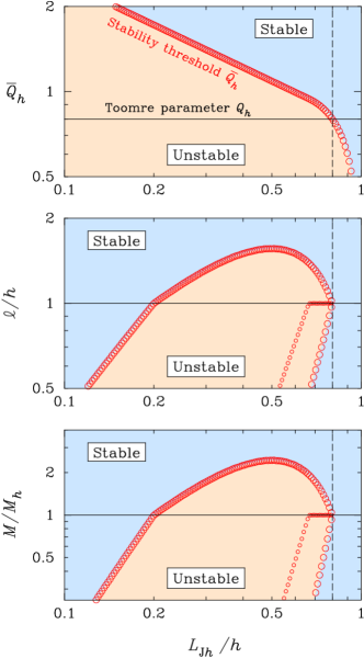
Figure 4: Stability properties of clumpy discs at high redshift: effect of a break in the mass-size scaling relation. The three panels show the stability threshold (top), the size range of unstable regions and the most unstable scale (middle), and the associated masses (bottom). The clump scaling relations are $\sigma(\ell)=\sigma_{h}(\ell/h)^{1/2}$, $\Sigma(\ell)=\Sigma_{h}(\ell/h)^{1/3}$ if $\ell\leq h$ and $\Sigma(\ell)=\Sigma_{h}$ otherwise, where $h$ is the disc scale height. This is suggested by observations and simulations of galactic turbulence (see Sect. 3). $Q_{h}\equiv\kappa\sigma_{h}/\pi G\Sigma_{h}$ and $L_{\mathrm{J}h}\equiv\sigma_{h}^{2}/G\Sigma_{h}$ are the Toomre parameter and the 2D Jeans length at scale $\ell=h$. The case $Q_{h}=0.8$ is shown for illustrative purposes. Qualitatively similar results are found for all values of $Q_{h}\la 1$ (see again Sect. 3).

So what role does the disc scale height play in our stability scenario? To answer this question, we consider the following mass-size and linewidth-size scaling relations:

$$\Sigma(\ell)=\Sigma_{h}\left(\frac{\ell}{h}\right)^{a},\;\;\;\;\;a=\left\{\begin{array}[]{ll}1/3&\mbox{if\ }\ell\leq h\,,\\ 0&\mbox{else}\,;\end{array}\right.$$ (10)

$$\sigma(\ell)=\sigma_{h}\left(\frac{\ell}{h}\right)^{b},\;\;\;\;\;b=1/2\,.$$ (11)

Such values of $a$ and $b$ are motivated by the results discussed above, and by the detailed comparative analysis carried out by Kritsuk et al. (2013) for $\ell\la h$ (see Sect. 2.3). Fig. 4 illustrates that a break in the mass-size scaling relation causes a transition in the stability properties of the disc. Look for example at the middle panel, and see how the size range of unstable regions and the most unstable scale ‘break’ at $\ell=h$. Such a transition exists for all values of $Q_{h}\la 1$, and should be observable if the disc scale height is spatially resolved. Note also that the characteristic instability scale for marginally unstable discs ($Q_{h}=\overline{Q}_{h}$) is

$$\ell_{\mathrm{c}}=h\approx L_{\mathrm{J}h}\,.$$ (12)

This means that the disc scale height is also the natural size of unstable clumps, and is comparable to the 2D Jeans length (for $Q_{h}=\overline{Q}_{h}$). Is this an obvious result? No, it is not! In non-clumpy but realistically thick gas discs, the characteristic instability scale is

$$\ell_{\mathrm{c}}\approx 4\pi h=4L_{\mathrm{J}}$$ (13)

(see Appendix A). This is well beyond the ranges shown in Fig. 4.

The results discussed above show that the disc scale height plays an important role in our stability scenario. This is a promising and novel avenue for constraining the size and mass of star-forming clumps in high-redshift galaxies, a topic that we will address further in future work.

4 SUMMARY AND CONCLUSIONS

We have investigated the gravitational instability of clumpy disc galaxies, focusing on the size and mass ranges of unstable regions. Multi-frequency observations of both the gas and the stellar contents (e.g., Elmegreen & Elmegreen 2006; Shapiro et al. 2008; Tacconi et al. 2010) have established that such galaxies are ubiquitous at high redshift. Furthermore, the majority of stars in the Universe are known to form at $z>1$ (e.g., Hopkins & Beacom 2006). Thus it is crucial to understand the properties of unstable star-forming gas at this epoch of galaxy evolution.

Clumpy discs at high redshift are dynamically similar to gas discs with scale-dependent surface density and velocity dispersion, i.e. $\Sigma\propto\ell^{a}$ and $\sigma\propto\ell^{b}$, where $\ell$ is the clump size. Taking these ‘turbulent’ scaling relations into account, and extending the traditional Toomre stability analysis as in Romeo et al. (2010), a wide variety of non-classical stability properties arise. We have illustrated this scenario for the whole observed range spanned by the clump scaling relations, which is centred around Larson’s scaling laws $(a,b)=(0,\frac{1}{2})$, and for a range of spatial resolution scales typical of current high-redshift surveys. Our key results and a few eloquent examples are summarized below.

1. The scale-dependence of the surface density and velocity dispersion plays a crucial role in determining the size and mass ranges of unstable regions. For example, in the rings and outer discs of SINS/zC-SINF galaxies at $z\sim 2$ (Genzel et al. 2014), where the spatial resolution scale is close to the inferred 2D Jeans length, small variations in the logarithmic slope of $\Sigma(\ell)$ can lead to dramatic, order-of-magnitude, changes in the mass of the most unstable clumps. For the same observed surface density and velocity dispersion, logarithmic slopes of $\sigma(\ell)$ steeper than $b\approx 0.4$ and flatter than $b\approx 0.5$ ($a=0$) lead to complete disc stability. This illustrates the dynamical complexity introduced by the clump scaling relations.

2. Variations in the logarithmic slopes of $\Sigma(\ell)$ and $\sigma(\ell)$ can drive significant changes in the stability properties of the disc at all scales. For example, a clumpy disc can be marginally stable even if the classical Toomre parameter $Q_{0}\ll 1$. In the case of Larson’s scaling laws, the disc is always stable, however small $Q_{0}$ is, if the inferred 2D Jeans length $L_{\mathrm{J}0}$ is larger than the spatial resolution scale $\ell_{0}$.

3. For discs with $Q_{0}=1$, we have payed special attention to $b\approx 0.5$ and $-0.1\la a\la 0.6$, since this range encompasses the most representative values of $a$ and $b$ found in observational (e.g., Larson 1981; Solomon et al. 1987) and theoretical (e.g., Federrath 2013; Kritsuk et al. 2013) works on supersonic turbulence. In spite of being marginally stable in the classical sense, such discs can be anywhere from highly stable to unstable, depending on the value of $a$. In fact, as $a$ approaches 0.6 while $L_{\mathrm{J}0}=\ell_{0}$, all observable scales $\ell\ga 2L_{\mathrm{J}0}$ become unstable, even though the disc is close to the stability threshold ($\overline{Q}_{0}\approx 1.1$).

Points (i)–(iii) illustrate the peculiar stability regimes possessed by discs with scale-dependent surface densities and velocity dispersions, and why it is important to take such regimes into account when predicting the size and mass of star-forming clumps in high-redshift galaxies. Note also that our work raises an important caveat: as the interstellar medium (ISM) is characterized by scale-dependent surface densities and velocity dispersions, we cannot thoroughly understand its global stability properties unless we carry out multi-scale observations. This will soon be possible thanks to dedicated ALMA surveys, which will explore the physical properties of super-giant molecular clouds at the peak of cosmic star formation and beyond.

Our work provides a new set of tools for exploring galactic star formation. In the ISM, there exist different sources of turbulence driving, such as large-scale gravitational stirring and stellar feedback (e.g., Mac Low & Klessen 2004; Agertz et al. 2009a), and it is still unclear how they affect the ISM at various scales. Understanding the origin and evolution of $a$ and $b$, and how they vary with galactic environment, is a daunting task for numerical simulations, given the vast dynamical range involved in the star-forming ISM: from scales $\ell\la 0.1\,\mbox{pc}$ to scales $\ell\sim 10\,\mbox{kpc}$. Preliminary results from numerical simulations of entire galactic discs (Agertz, Romeo & Grisdale, in preparation) show that large-scale gravitational stirring and stellar feedback can generate markedly different scaling properties in both $\Sigma(\ell)$ and $\sigma(\ell)$. This is a promising and novel avenue for constraining the role of stellar feedback in galaxy evolution, a topic that we will address further in future work.

Appendix A DERIVATION OF EQ. (13)

Consider a gas disc of scale height $h$, and perturb it with axisymmetric waves of frequency $\omega$ and wavenumber $k$. The response of the disc is described by the dispersion relation

$$\omega^{2}=\kappa^{2}-\frac{2\pi G\Sigma\,k}{1+kh}+\sigma^{2}\,k^{2}\,,$$ (14)

where $\kappa$ is the epicyclic frequency, $\Sigma$ is the surface density at equilibrium, and $\sigma$ is the 1D velocity dispersion (Vandervoort 1970; Romeo 1992, 1994; Elmegreen 2011; Griv & Gedalin 2012 extended this analysis to non-axisymmetric waves). So the three terms on the right side of Eq. (A1) represent the contributions of rotation, self-gravity and pressure. For $kh\ll 1$, Eq. (A1) reduces to the usual dispersion relation for an infinitesimally thin gas disc. For $kh\gg 1$, one recovers the case of Jeans instability with rotation, since $\Sigma/h=2\rho$. In other words, scales comparable to $h$ mark the transition from 2D to 3D stability.

If the disc is self-gravitating and isothermal along the vertical direction, as assumed in the analyses above, then the disc scale height is closely related to the 2D Jeans length:

$$h=\frac{\sigma^{2}}{\pi G\Sigma}=\frac{L_{\mathrm{J}}}{\pi}\,.$$ (15)

To compute the characteristic instability scale, we express the dispersion relation in a form similar to Eq. (9):

$$\frac{\omega^{2}}{\kappa^{2}}=1-\frac{4}{Q^{2}}\,\frac{1}{2+(\ell/L_{\mathrm{J}})}+\frac{4}{Q^{2}}\,\frac{1}{(\ell/L_{\mathrm{J}})^{2}}\,.$$ (16)

The most unstable scale is the scale that minimizes the dispersion relation: $\ell_{\mathrm{min}}\approx 4L_{\mathrm{J}}$. In this classical case, $\ell_{\mathrm{min}}$ does not depend on whether the disc is marginally unstable or not, and is therefore the characteristic instability scale:

$$\ell_{\mathrm{c}}=\ell_{\mathrm{min}}\approx\frac{4\sigma^{2}}{G\Sigma}\,.$$ (17)

Using Eq. (A2), we find that

$$\ell_{\mathrm{c}}\approx 4\pi h=4L_{\mathrm{J}}\,,$$ (18)

which is Eq. (13) of the main text.

References

- [1] Agertz O., Lake G., Teyssier R., Moore B., Mayer L., Romeo A. B., 2009a, MNRAS, 392, 294
- [2] Agertz O., Teyssier R., Moore B., 2009b, MNRAS, 397, L64
- [3] Beaumont C. N., Goodman A. A., Alves J. F., Lombardi M., Román-Zúñiga C. G., Kauffmann J., Lada C. J., 2012, MNRAS, 423, 2579
- [4] Beaumont C. N., Offner S. S. R., Shetty R., Glover S. C. O., Goodman A. A., 2013, ApJ, 777, 173
- [5] Behroozi P. S., Wechsler R. H., Conroy C., 2013, ApJ, 762, L31
- [6] Bertram E., Shetty R., Glover S. C. O., Klessen R. S., Roman-Duval J., Federrath C., 2014, MNRAS, 440, 465
- [7] Block D. L., Puerari I., Elmegreen B. G., Bournaud F., 2010, ApJ, 718, L1
- [8] Bournaud F., Elmegreen B. G., Elmegreen D. M., 2007, ApJ, 670, 237
- [9] Bournaud F., Elmegreen B. G., Teyssier R., Block D. L., Puerari I., 2010, MNRAS, 409, 1088
- [10] Burkert A. et al., 2010, ApJ, 725, 2324
- [11] Cacciato M., Dekel A., Genel S., 2012, MNRAS, 421, 818
- [12] Carilli C. L., Walter F., 2013, ARA&A, 51, 105
- [13] Ceverino D., Dekel A., Bournaud F., 2010, MNRAS, 404, 2151
- [14] Collins D. C., Kritsuk A. G., Padoan P., Li H., Xu H., Ustyugov S. D., Norman M. L., 2012, ApJ, 750, 13
- [15] Combes F. et al., 2012, A&A, 539, A67
- [16] Daddi E. et al., 2010, ApJ, 713, 686
- [17] Dekel A., Sari R., Ceverino D., 2009, ApJ, 703, 785
- [18] Donovan Meyer J. et al., 2013, ApJ, 772, 107
- [19] Dutta P., Begum A., Bharadwaj S., Chengalur J. N., 2009, MNRAS, 397, L60
- [20] Elmegreen B. G., 2011, ApJ, 737, 10
- [21] Elmegreen B. G., Elmegreen D. M., 2006, ApJ, 650, 644
- [22] Elmegreen B. G., Kim S., Staveley-Smith L., 2001, ApJ, 548, 749
- [23] Elmegreen B. G., Bournaud F., Elmegreen D. M., 2008, ApJ, 688, 67
- [24] Elmegreen B. G., Elmegreen D. M., Fernandez M. X., Lemonias J. J., 2009, ApJ, 692, 12
- [25] Elmegreen D. M., Elmegreen B. G., Ravindranath S., Coe D. A., 2007, ApJ, 658, 763
- [26] Federrath C., 2013, MNRAS, 436, 1245
- [27] Federrath C., Klessen R. S., Schmidt W., 2009, ApJ, 692, 364
- [28] Federrath C., Roman-Duval J., Klessen R. S., Schmidt W., Mac Low M.-M., 2010, A&A, 512, A81
- [29] Forbes J., Krumholz M., Burkert A., 2012, ApJ, 754, 48
- [30] Forbes J. C., Krumholz M. R., Burkert A., Dekel A., 2014, MNRAS, 438, 1552
- [31] Fujimoto Y., Tasker E. J., Wakayama M., Habe A., 2014, MNRAS, 439, 936
- [32] Genzel R. et al., 2011, ApJ, 733, 101
- [33] Genzel R. et al., 2014, ApJ, 785, 75
- [34] Glazebrook K., 2013, PASA, 30, 56
- [35] Griv E., Gedalin M., 2012, MNRAS, 422, 600
- [36] Hennebelle P., Falgarone E., 2012, A&ARv, 20, 55
- [37] Hoffmann V., Romeo A. B., 2012, MNRAS, 425, 1511
- [38] Hopkins A. M., Beacom J. F., 2006, ApJ, 651, 142
- [39] Kauffmann J., Pillai T., Goldsmith P. F., 2013, ApJ, 779, 185
- [40] Kim S. et al., 2007, ApJS, 171, 419
- [41] Kritsuk A. G., Lee C. T., Norman M. L., 2013, MNRAS, 436, 3247
- [42] Kruijssen J. M. D., Longmore S. N., 2013, MNRAS, 435, 2598
- [43] Krumholz M., Burkert A., 2010, ApJ, 724, 895
- [44] Larson R. B., 1979, MNRAS, 186, 479
- [45] Larson R. B., 1981, MNRAS, 194, 809
- [46] Lazarian A., Pogosyan D., 2000, ApJ, 537, 720
- [47] Leroy A. K., Walter F., Brinks E., Bigiel F., de Blok W. J. G., Madore B., Thornley M. D., 2008, AJ, 136, 2782
- [48] Mac Low M.-M., Klessen R. S., 2004, Rev. Mod. Phys., 76, 125
- [49] Noguchi M., 1998, Nature, 392, 253
- [50] Noguchi M., 1999, ApJ, 514, 77
- [51] Overzier R. A. et al., 2008, ApJ, 677, 37
- [52] Puech M., 2010, MNRAS, 406, 535
- [53] Romeo A. B., 1992, MNRAS, 256, 307
- [54] Romeo A. B., 1994, A&A, 286, 799
- [55] Romeo A. B., Falstad N., 2013, MNRAS, 433, 1389
- [56] Romeo A. B., Burkert A., Agertz O., 2010, MNRAS, 407, 1223
- [57] Sánchez N., Añez N., Alfaro E. J., Odekon M. C., 2010, ApJ, 720, 541 (Erratum in ApJ, 723, 969)
- [58] Shapiro K. L. et al., 2008, ApJ, 682, 231
- [59] Shetty R., Beaumont C. N., Burton M. G., Kelly B. C., Klessen R. S., 2012, MNRAS, 425, 720
- [60] Solomon P. M., Rivolo A. R., Barrett J., Yahil A., 1987, ApJ, 319, 730
- [61] Swinbank A. M. et al., 2011, ApJ, 742, 11
- [62] Tacconi L. J. et al., 2010, Nature, 463, 781
- [63] Vandervoort P. O., 1970, ApJ, 161, 87
- [64] Ward R. L., Wadsley J., Sills A., 2014, MNRAS, 439, 651
- [65] Weinmann S. M., Neistein E., Dekel A., 2011, MNRAS, 417, 2737
- [66] Wisnioski E., Glazebrook K., Blake C., Poole G. B., Green A. W., Wyder T., Martin C., 2012, MNRAS, 422, 3339