Clique counting in MapReduce:
theory and experiments

Abstract

We tackle the problem of counting the number of $k$-cliques in large-scale graphs, for any constant $k\geq 3$. Clique counting is essential in a variety of applications, among which social network analysis. Due to its computationally intensive nature, we settle for parallel solutions in the MapReduce framework, which has become in the last few years a de facto standard for batch processing of massive data sets. We give both theoretical and experimental contributions.

On the theory side, we design the first exact scalable algorithm for counting (and listing) $k$-cliques. Our algorithm uses $O(m^{3/2})$ total space and $O(m^{k/2})$ work, where $m$ is the number of graph edges. This matches the best-known bounds for triangle listing when $k=3$ and is work-optimal in the worst case for any $k$, while keeping the communication cost independent of $k$. We also design a sampling-based estimator that can dramatically reduce the running time and space requirements of the exact approach, while providing very accurate solutions with high probability.

We then assess the effectiveness of different clique counting approaches through an extensive experimental analysis over the Amazon EC2 platform, considering both our algorithms and their state-of-the-art competitors. The experimental results clearly highlight the algorithm of choice in different scenarios and prove our exact approach to be the most effective when the number of $k$-cliques is large, gracefully scaling to non-trivial values of $k$ even on clusters of small/medium size. Our approximation algorithm achieves extremely accurate estimates and large speedups, especially on the toughest instances for the exact algorithms. As a side effect, our study also sheds light on the number of $k$-cliques of several real-world graphs, mainly social networks, and on its growth rate as a function of $k$.

Keywords: Clique listing, graph algorithms, MapReduce, parallel algorithms, experimental algorithmics

1 Introduction

The problem of counting small subgraphs with specific structural properties in large-scale networks has gathered a lot of interest from the research community during the last few years. Counting – and possibly listing – all instances of triangles, cycles, cliques, and other different structures is indeed a fundamental tool for uncovering the properties of complex networks [24], with wide-ranging applications that include spam and anomaly detection [6, 14], social network analysis [17, 31], and the discovery of patterns in biological networks [32].

Since many interesting graphs have by themselves really large sizes, developing analysis algorithms that scale gracefully on such instances is rather challenging. Designing efficient sequential algorithms is often not enough: even assuming that the input graphs could fit into the memory of commodity hardware, subgraph counting is a computationally intensive problem and the running times of sequential algorithms can easily become unacceptable in practice. To overcome these issues, many recent works have focused on speeding up the computation by exploiting parallelism (e.g., using MapReduce [13]), by working in external memory models [37], or by settling for approximate – instead of exact – answers (as done, e.g., in data streaming [25]).

In this paper we tackle the problem of counting the number of $k$-cliques in large-scale graphs, for any constant $k\geq 3$. This is a fundamental problem in social network analysis (see, e.g., [17] – Chapter 11) and algorithms that produce a census of all cliques are also included in widely-used software packages, such as UCINET [8]. We present simple and scalable algorithms suitable to be implemented in the MapReduce framework [13] that, together with its open source implementation Hadoop [3], has become a de facto standard for programming massively distributed systems both in industry and academia. MapReduce indeed offers programmers the possibility to easily run their code on large clusters while neglecting any issues related to scheduling, synchronization, communication, and error detection (that are automatically handled by the system). Computational models for analyzing MapReduce algorithms are described in [21, 15, 30].

$k$-clique counting is a natural generalization of triangle counting, where $k=3$: this is the simplest, non-trivial version of the problem and has been widely studied in the literature. Appendix A describes related works in a variety of models of computation. Focusing on MapReduce, two different exact algorithms for listing triangles have been proposed by Suri and Vassilvitskii [35] and validated on real world datasets. One of these algorithms has been recently extended to count arbitrary subgraphs by Afrati et al. [1], casting it into a general framework based on the computation of multiway joins. A sampling-based randomized approach whose output estimate is strongly concentrated around the true number of triangles (under mild conditions) has been finally described by Pagh and Tsourakakis in [28]. We remark that subgraph counting becomes more and more computationally demanding as the number $k$ of nodes in the counted subgraph gets larger, due to the combinatorial explosion of the number of candidates. This is especially true for $k$-cliques, as we will also show in this paper, since certain real world graphs (such as social networks) are characterized by high clustering coefficients and very large numbers of small cliques.

Our results.

The contribution in this paper is two-fold and includes both theoretical and experimental results. On the theory side, we design and analyze the first scalable exact algorithm for counting (and listing) $k$-cliques as well as sampling-based approximate solutions. In more details:

• Our exact $k$-clique counting algorithm uses $O(m^{3/2})$ total space and $O(m^{k/2})$ work, where $m$ is the number of graph edges. The local space and the local running time of mappers and reducers are $O(m)$ and $O(m^{(k-1)/2})$, respectively. For $k=3$, total space and work match the bounds for triangle counting achieved in [35]. Similarly to the multiway join algorithm from [1], our algorithm is work-optimal in the worst case for any $k$. However, our total space is proportional to $m^{3/2}$ regardless of $k$: this means that, differently from [1], the communication cost does not grow when $k$ gets larger.

• Our sampling-based estimators reduce dramatically running time and local space requirements of the exact approach, while providing very accurate solutions w.h.p. These algorithms can be proved to belong to the class $\mathcal{MRC}$ [21] for a suitable choice of the probability parameters. For $k=3$, our concentration results require weaker conditions than the triangle counting algorithm from [28].

To assess the effectiveness of different clique counting approaches, we conducted a thorough experimental analysis over the Amazon EC2 platform, considering both our algorithms and those described in [1] and [35]. We used publicly available real data sets taken from the SNAP graph library [34] and synthetic graphs generated according to the preferential attachment model [5]. As a side effect, our experimental study also sheds light on the number of $k$-cliques of several SNAP datasets and on its growth rate as a function of $k$. The outcome of our experiments can be summarized as follows:

• Even for small values of $k$, some of the input graphs contain a number $q_{k}$ of $k$-cliques that can be in the order of tens or hundreds of trillions (recall that a trillion is $10^{12}$): in these cases, the output of the $k$-clique listing problem could easily require Terabytes or even Petabytes of storage (assuming no compression). As $k$ increases, we witnessed different growth rates of $q_{k}$ for different graph instances: while on some graphs $q_{k+1}<q_{k}$ (even for small values of $k$), on other instances $q_{k+1}\gg q_{k}$, up to two orders of magnitude in our observations. Graphs with a quick growth of the number of $k$-cliques represent particularly tough instances in practice.

• Among the exact algorithms considered in our analysis, our approach proves to be the most effective when the number of $k$-cliques is large. There are cases where it is outperformed by the triangle counting algorithm of [35] and by the multiway join algorithm of [1]: this happens either for $k=3,4$ or on “easy” instances where parallelization does not pay off (we observed that in these cases a simple sequential algorithm would be even faster). On the tough instances, however, our algorithm can gracefully scale as $k$ gets larger, differently from the multiway join approach [1]. We provide a theoretical justification of these experimental findings.

• Our approximate algorithms exhibit rather stable running times on all graphs for the considered values of $k$, and make it possible to solve in a few minutes instances that were impossible to be solved exactly. The quality of the approximation is extremely good: the error is around $0.08\%$ on average, with more accurate estimates on datasets that are more challenging for the exact algorithms. The variance across different executions, even on different clusters, also appears to be negligible.

Overall, the experiments show the practical effectiveness of our algorithms even on clusters of small/ medium size, and suggest their scalability to larger clusters. The full experimental package is available at https://github.com/CliqueCounter/QkCount/ for the purpose of repeatability.

2 Preliminaries

Throughout this paper we denote by $q_{k}$ the number of cliques on $k$ nodes. For a given graph $G$ and any node $u$ in $G$, $\Gamma(u)$ is the set of neighbors of node $u$ ($u$ is not included); moreover $d(u)=|\Gamma(u)|$. We define a total order $\prec$ over the nodes of $G$ as follows: $\forall x,y\in V(G)$, $x\prec y$ iff $d(x)<d(y)$ or $d(x)=d(y)$ and $x<y$ (we assume nodes to have comparable labels). Denote by $\Gamma^{+}(u)\subseteq\Gamma(u)$ the high-neighborhood of node $u$, i.e., the set of neighbors $x$ of $u$ such that $u\prec x$; symmetrically, $\Gamma^{-}(u)=\Gamma(u)\setminus\Gamma^{+}(u)$. Given two graphs $G(V,E)$ and $G_{1}(V_{1},E_{1})$, $G_{1}$ is a subgraph of $G$ if $V_{1}\subseteq V$ and $E_{1}\subseteq E$. $G_{1}$ is an induced subgraph of $G$ if, in addition to the above conditions, for each $u,v\in V_{1}$ it also holds: $(u,v)\in E_{1}$ if and only if $(u,v)\in E$. We denote the subgraph induced by the high-neighborhood $\Gamma^{+}(u)$ of a node $u$ as $G^{+}(u)$. Our algorithms do not require graphs to be connected. However, since their input is given as a set of edges and isolated nodes are irrelevant for clique counting, we can assume $n\leq 2m$. Moreover, we assume the endpoints of each edge to be labeled with their degree (the degree of each node can be precomputed in MapReduce very efficiently [21]). Additional preliminary results used in our proofs are given in Appendix B.

MapReduce. A MapReduce program is composed of (usually a small number of) rounds. Each round is conceptually divided into three consecutive phases: map, shuffle, and reduce. Input/output values of a round, as well as intermediate data exchanged between mappers and reducers, are stored as $\langle key;value\rangle$ pairs. In the map phase pairs are arbitrarily distributed among mappers and a programmer-defined map function is applied to each pair. Mappers are stateless and process each input pair independently from the others. The shuffle phase is transparent to the programmer: during this phase, the intermediate output pairs emitted by the mappers are grouped by key. All pairs with the same key are then sent to the same reducer, that will process each of them by executing a programmer-defined reduce function. Parallelism comes from concurrent execution of mappers as well as reducers. The authors of [21] made an effort to pinpoint the critical aspects of efficient MapReduce algorithms. In particular: (1) the memory used by a single mapper/reducer should be sublinear with respect to the total input size (this allows to exclude trivial algorithms that simply map the whole input to a single reducer, which then solves the problem via a sequential algorithm); (2) the total number of machines available should be sublinear in the data size; (3) both the map and the reduce functions should run in polynomial time with respect to the original input length. The model also requires programs to be composed of a polylogarithmic number of rounds, since shuffling is a time consuming operation, and to have a total memory usage (which coincides with the communication cost from [1] for the purpose of this paper) that grows substantially less than quadratically with respect to the input size. Algorithms respecting these conditions are said to belong to the class $\mathcal{MRC}$.

3 Exact counting

Our algorithms use the total order $\prec$ to decide which node of a given clique $Q$ is responsible for counting $Q$. In particular, $Q$ is counted by its smallest node, i.e., the node $u\in Q$ such that $u\prec x$, for all $x\in Q\setminus\{u\}$. At a high level, the strategy is to split the whole graph in many subgraphs, namely the subgraphs $G^{+}(u)$ induced by $\Gamma^{+}(u)$, for each $u\in V(G)$, and count the cliques in each subgraph independently (both nodes and edges of $G$ can appear in more than one subgraph). Our counting algorithm, called FFF_k, works in three rounds (see Algorithm 1 for the pseudocode):

Map 1: input $\langle(u,v);\emptyset\rangle$

  if $u\prec v$ then emit $\langle u;v\rangle$

Reduce 1: input $\langle u;\Gamma^{+}(u)\rangle$

  if $|\Gamma^{+}(u)|\geq k-1$ then emit $\langle u;\Gamma^{+}(u)\rangle$

Map 2: input $\langle u;\Gamma^{+}(u)\rangle$ or $\langle(u,v);\emptyset\rangle$

  if input of type $\langle(u,v);\emptyset\rangle$ and $u\prec v$ then

     emit $\langle(u,v);\$)\rangle$

  if input of type $\langle u;\Gamma^{+}(u)\rangle$ then

     for each $x_{i},\,x_{j}\in\Gamma^{+}(u)$ s.t. $x_{i}\prec x_{j}$ do

        emit $\langle(x_{i},x_{j});u\rangle$

Reduce 2: input $\langle(x_{i},x_{j});\{u_{1},\ldots,u_{k}\}\cup\mbox{\$}\rangle$

  if input contains $ then

     emit $\langle(x_{i},x_{j});\{u_{1},\ldots,u_{k}\}\rangle$

Map 3: input $\langle(x_{i},x_{j});\{u_{1},\ldots,u_{k}\}\rangle$

  for $h\in[1,k]$ do

     emit $\langle u_{h};(x_{i},x_{j})\rangle$

Reduce 3: input $\langle u;G^{+}(u)\rangle$

  let $q_{u,k-1}=$ number of $(k-1)$-cliques in $G^{+}(u)$

  emit $\langle u;q_{u,k-1}\rangle$

Algorithm 1 : FFF_k

Round 1:

high-neighborhood computation. The computation of $\Gamma^{+}(u)$, for all nodes $u$ in $G$, exploits the degree information attached to the edges; mappers emit the pair $\langle x;y\rangle$ for each edge $(x,y)$ such that $x\prec y$, thus allowing the reduce instance with key $u$ to aggregate all nodes $x\in\Gamma^{+}(u)$.

Round 2:

small-neighborhoods intersection. The aim of the round is to associate each edge $(x,y)$ with $\Gamma^{-}(x)\cap\Gamma^{-}(y)$, i.e., with the set of nodes $u$ such that $G^{+}(u)$ contains $(x,y)$. This is done as follows. The map instance with input $\langle u;\Gamma^{+}(u)\rangle$ emits a pair $\langle(x,y);u\rangle$ for each pair $(x,y)\in\Gamma^{+}(u)\times\Gamma^{+}(u)$ such that $x\prec y$. Besides the output of round 1, similarly to [35] mappers are fed with the original set of edges and emit a pair $\langle(x,y);\$\rangle$ for each edge $(x,y)$ with $x\prec y$. This allows the reduce instance with key $(x,y)$ to check whether $(x,y)$ is an edge by looking for symbol $\$$ among its input values. At the same time this instance would receive the set $\Gamma^{-}(x)\cap\Gamma^{-}(y)$, which is exactly the set of nodes $u$ needing edge $(x,y)$ to construct $G^{+}(u)$.

Round 3:

($k-1$)-clique counting in high-neighborhoods. For each node $u$, count the number of $k$-cliques for which $u$ is responsible. Map instances correspond to graph edges. The map instance with key $(x,y)$ emits a pair $\langle u;(x,y)\rangle$ for each node $u\in\Gamma^{-}(x)\cap\Gamma^{-}(y)$. After shuffling, the reduce instance with key $u$ receives as input the whole list of edges between nodes in $\Gamma^{+}(u)$. Hence, it can reconstruct the subgraph $G^{+}(u)$ induced by the high-neighbors of $u$ and, by counting the $(k-1)$-cliques in this graph, can compute locally the number of $k$-cliques for which $u$ is responsible.

Notice that the round 3 reducers could be easily modified to output, for each node $v$, the number of cliques in which $v$ is contained, so that the overall number of cliques containing $v$ could be obtained by summing up the contributions from each subgraph $G^{+}(u)$. The following theorem, proved in Appendix B, analyzes work and space usage of FFF_k:

Theorem 1.

Let $G$ be a graph and let $m$ be the number of its edges. Algorithm FFF_k counts the number of $k$-cliques of $G$ using $O(m^{3/2})$ total space and $O(m^{k/2})$ work. The local space and the local running time of mappers and reducers are $O(m)$ and $O(m^{(k-1)/2})$, respectively.

With respect to the requirements defined in [21], algorithm FFF_k does not fit in the class $\mathcal{MRC}$ due to the local space requirements of reduce 2, map 3, and reduce 3 instances. These are linear in $n$ or $m$ whereas the $\mathcal{MRC}$ class requires them to be in $O(m^{1-\varepsilon})$, for some small constant $\varepsilon>0$. However, as we will see from the experimental evaluation we performed, local memory did not show any criticality in practice, whereas local complexity (which is almost completely neglected in the class $\mathcal{MRC}$) and global work proved to be the real challenge, since they can grow significantly as $k$ gets larger. Our approximate algorithms presented in Section 6 overcome these issues.

Similarly to the triangle counting algorithms from [35] and to the multiway join subgraph counting algorithm from [1], cast to the specific case of cliques (in short, AFU_k), the work of FFF_k is optimal with respect to the clique listing problem. Moreover, the total space of FFF_k is $\Theta(m^{3/2})$ regardless of $k$, matching the triangle counting bound of the Node Iterator ++ algorithm from [35] when $k=3$. Conversely, both AFU_k and the straightforward generalization to $k$-cliques of the Partition algorithm from [35] have a communication cost that depends both on a number $b$ of buckets, chosen as a parameter, and on the number $k$ of clique nodes (see [1] and [35] for details). In AFU_k, reducers are identified by $k$-tuples of buckets $\langle b_{i}\leq b_{2}\leq\ldots\leq b_{k}\rangle$. Each edge corresponds to a pair $\langle i,j\rangle$ of buckets (those to which its endpoints are hashed) and is sent to all the reducers whose $k$-tuple contains both $i$ and $j$. Each edge is thus replicated $\Omega(b^{k-2})$ times, for an overall communication cost $\Theta(m\cdot b^{k-2})$. Similar arguments apply to the generalization of Partition. We will see the implications in Section 5. We also notice that, differently from AFU_k and Partition, algorithm FFF_k needs no parameter tuning.

4 Experimental setup

Algorithms and implementation details. Besides algorithm FFF_k, we included in our test suite the Node Iterator ++ triangle counting algorithm from [35] (called SV) and the one-round subgraph counting algorithm AFU_k based on multiway joins [1], cast to $k$-cliques. We did not consider the Partition algorithm from [35] because AFU₃ is its optimized version. Both the reduce 3 instances of FFF_k and the reducers of AFU_k use as a subroutine an efficient clique counting algorithm based on neighborhood intersection, inspired by the fastest (optimal) triangle listing algorithm described in [26]. In the case of AFU_k, we took care of exploiting bucket orderings to discard as soon as possible $k$-cliques that do not fit in the $k$-tuple of a given reducer. According to our tests, this results in slightly faster running times w.r.t. to the plain version. All the implementations have been realized in Java using Hadoop 2.2.0. The code is instrumented so as to collect detailed statistics of map/reduce instances at each round, including sizes of the subgraphs involved in a computation (e.g., $|\Gamma^{+}(u)|$, $|\Gamma^{-}(x)\cap\Gamma^{-}(y)|$, and $|G^{+}(u)|$) and detailed running times. The algorithms have been tested in a variety of settings, using different parameter choices, instance families, and cluster configurations, as described below.

	$n$ ($=q_{1}$)	$m$ ($=q_{2}$)	$q_{3}$	$q_{4}$	$q_{5}$	$q_{6}$	$q_{7}$
citPat	$3.8\times 10^{6}$	$1.6\times 10^{7}$	$7.5\times 10^{6}$	$3.5\times 10^{6}$	$3.0\times 10^{6}$	$3.1\times 10^{6}$	$1.9\times 10^{6}$
youTube	$1.1\times 10^{5}$	$3.0\times 10^{6}$	$3.0\times 10^{6}$	$5.0\times 10^{6}$	$7.2\times 10^{6}$	$8.4\times 10^{6}$	$8.0\times 10^{6}$
locGowalla	$2.0\times 10^{5}$	$9.5\times 10^{5}$	$2.7\times 10^{6}$	$6.1\times 10^{6}$	$1.5\times 10^{7}$	$2.9\times 10^{7}$	$4.8\times 10^{7}$
socPokec	$1.6\times 10^{6}$	$2.2\times 10^{7}$	$3.3\times 10^{7}$	$4.3\times 10^{7}$	$5.3\times 10^{7}$	$6.5\times 10^{7}$	$8.4\times 10^{7}$
webGoogle	$8.7\times 10^{5}$	$4.3\times 10^{6}$	$1.3\times 10^{7}$	$3.4\times 10^{7}$	$1.0\times 10^{8}$	$2.5\times 10^{8}$	$6.0\times 10^{8}$
webStan	$2.8\times 10^{5}$	$2.0\times 10^{6}$	$1.1\times 10^{7}$	$7.9\times 10^{7}$	$6.2\times 10^{8}$	$4.9\times 10^{9}$	$3.5\times 10^{10}$
asSkit	$1.7\times 10^{6}$	$1.1\times 10^{7}$	$2.9\times 10^{7}$	$1.5\times 10^{8}$	$1.2\times 10^{9}$	$9.8\times 10^{9}$	$7.3\times 10^{10}$
orkut	$3.1\times 10^{6}$	$1.2\times 10^{8}$	$6.3\times 10^{8}$	$3.2\times 10^{9}$	$1.6\times 10^{10}$	$7.5\times 10^{10}$	$3.5\times 10^{11}$
webBerkStan	$6.8\times 10^{5}$	$6.6\times 10^{6}$	$6.5\times 10^{7}$	$1.1\times 10^{9}$	$2.2\times 10^{10}$	$4.6\times 10^{11}$	$9.4\times 10^{12}$
comLiveJ	$4.0\times 10^{6}$	$3.5\times 10^{7}$	$1.8\times 10^{8}$	$5.2\times 10^{9}$	$2.5\times 10^{11}$	$1.1\times 10^{13}$	4.4 $\times$ 1014
socLiveJ1	$4.8\times 10^{6}$	$4.3\times 10^{7}$	$2.9\times 10^{8}$	$9.9\times 10^{9}$	$4.7\times 10^{11}$	$2.1\times 10^{13}$	8.6 $\times$ 1014
egoGplus	$1.1\times 10^{5}$	$1.2\times 10^{7}$	$1.1\times 10^{9}$	$7.8\times 10^{10}$	$4.7\times 10^{12}$	2.4 $\times$ 1014	1.1 $\times$ 1016

Table 1: Benchmark statistics: order of magnitude of $n$, $m$, and $q_{k}$ (numbers of nodes, edges, and $k$-cliques, respectively) for $k\in[3,7]$. Clique numbers in italic are estimates obtained by the algorithm described in Section 6. The table in Appendix C shows the exact values and the clique growth rates.

Data sets. We used several real-world graphs from the SNAP graph library [34] as well as synthetic graphs generated according to the preferential attachment model [5]. We preprocessed all graphs so that they are undirected and each edge endpoint is associated with its degree. Degree computation is a common step to both SV and FFF_k, and can be done very easily and quickly in MapReduce [21]. Throughout the paper we report on the results obtained for a variety of online social networks (called orkut, socPokec, youTube, locGowalla, socLiveJ1, comLiveJ, egoGplus), Web graphs (webBerkStan, webGoogle, webStan), an Internet topology graph (asSkit), and a citation network among US Patents (citPat). The main characteristics of these datasets are summarized in Table 1. Notice that only the number $q_{3}$ of triangles was available from [34] before our study. With respect to $q_{3}$, the number of $k$-cliques for larger values of $k$ can grow considerably, up to the order of tens or even hundreds of trillions.

Platform. The experiments have been carried out on three different Amazon EC2 clusters, running Hadoop 2.2.0. Besides the master node, the three clusters included 4, 8, and 16 worker nodes, respectively, devoted to both Hadoop tasks and the HDFS. We used Amazon EC2 m3.xlarge instances, each providing 4 virtual cores, 7.5 GiB of main memory, and a 32 GB solid state disk. We set the number of reduce tasks to match the number of virtual cores in each cluster and disabled speculative execution. We also modified the memory requirements of the containers in order to improve load balancing on the cluster. The precise Hadoop configuration used on the Amazon clusters is provided with our experimental package available on github.

	SV	FFF3	AFU3	FFF4	AFU4	FFF5	AFU5	FFF6	AFU6	FFF7	AFU7
citPat	2:44	3:22	2:23	3:11	3:11	3:13	2:18	3:13	2:19	3:09	2:24
youTube	2:06	2:04	1:25	2:39	1:41	2:34	1:33	2:36	1:39	2:38	1:49
locGowalla	2:36	3:08	1:18	3:04	1:21	3:02	1:30	3:04	1:24	3:03	1:30
socPokec	4:03	4:15	2:18	4:02	2:29	4:13	2:39	4:15	2:51	4:09	3:02
webGoogle	2:13	2:44	1:23	2:43	1:27	2:43	1:32	2:40	1:40	2:40	1:52
webStan	2:02	2:39	1:15	2:29	1:27	2:37	2:06	2:36	4:00	2:05	14:12
asSkit	2:44	3:14	1:43	3:17	2:59	3:18	5:34	3:14	25:30	4:12	$>$40
orkut	30:07	24:00	8:21	23:08	20:17	23:10	$>$50	23:22	$>$50	28:08	-
webBerkStan	2:28	3:00	1:37	3:01	2:53	3:08	8:24	4:56	$>$30	50:17	-
comLiveJ	5:31	5:31	2:53	5:24	4:06	6:13	14:02	41:22	$>$170	-	-
socLiveJ1	6:36	6:33	3:14	6:43	5:10	7:51	23:35	86:34	$>$180	-	-
egoGplus	22:54	17:19	2:06	17:54	16:55	39:01	$>$90	-	-	-	-

Table 2: Running time (minutes:seconds) of the algorithms on a 16-node cluster with 64 total cores. To minimize the costs, we killed some executions of AFU_k that took more than twice the time of FFF_k. For the sake of comparison, the running times of algorithm SV reported in [35] are 1.90, 1.77, and 5.33 minutes on asSkit, webBerkStan, and socLiveJ1, respectively, on a 1636-node cluster.

5 Computational experiments

In this section we summarize our main experimental findings. We first present results obtained on a 16-node Amazon cluster, analyzing the effects of $k$ on the performance of the algorithms, and we then address scalability issues on different cluster sizes. Our experiments account for more than 60 hours of computation over the EC2 platform. Table 2 is the main outcome of this study, showing the running times of all the evaluated algorithms for $k\leq 7$ on the SNAP graphs ordered by increasing $q_{7}$ (see Appendix C). Results for synthetic instances were consistent with real datasets and are not reported.

Triangle counting: the costs of rounds. Since the overhead of setting up a round – including shuffling – is non-negligible in MapReduce, the one-round AFU₃ algorithm is always much faster than SV and FFF₃, which respectively require two and three rounds. FFF₃ is slower than SV on most datasets, but faster on orkut and egoGplus, which have the largest number of triangles (see also Table 1). We conjectured that this may be due to the early computation of length-$2$ paths performed in SV by the round 1 reducers (see [35] for details), which uselessly increases the communication cost of round 1. To test our hypothesis, we engineered a variant of SV that delays $2$-path computation to the map phase of round 2. The variant showed largely improved running times, solving orkut and egoGplus in 22 and 12 minutes (instead of 30 and 23, resp.) and being faster than FFF₃ on all benchmarks.

Running time analysis for $k\geq 4$. Algorithm FFF₄ can compute the number of $4$-cliques within roughly the same time required to count triangles. AFU₄ remains faster than FFF₄, but is always slower than AFU₃: see, in particular, orkut and egoGplus. In general, when $k\geq 5$, FFF_k proves to be more and more effective than AFU_k and its running times scale gracefully with $k$, especially on the most difficult instances characterized by a steep growth of the number of $k$-cliques (asSkit, the LiveJournal networks, orkut, webBerkStan, and egoGplus). To explain this behavior, recall that AFU_k requires to choose the number $b$ of buckets that, together with $k$, determines the number of reducers. The communication cost, as observed in Section 3, grows as $\Theta(m\cdot b^{k-2})$, which in practice calls for small values of $b$: if $b$ is too large, even a small input graph could quickly grow to Terabytes of disk usage for moderate values of $k$. On the other hand, since the local running times of reducers are inversely proportional to $b$, if $b$ is too small w.r.t. $k$ the worst-case reducers incur high running times (if, e.g., $k>b/2$, some $k$-tuple contains more than half of the buckets and the corresponding reducer will receive more than half of the total number of edges). The running times of such reducers (as well as their memory requirements) remain comparable to that of the sequential algorithm. The practical implication of this communication/runtime tradeoff is that the best performance of AFU_k have been obtained within our experimental setup using rather small values of $b$. We nevertheless performed experiments with different choices of $b$: as suggested in [1], we first set $b$ so that ${b+k-1}\choose k$ is as close as possible to the available reducers, and we then considered a variety of different values. Table 2 always reports the fastest running time that we could obtain by separately tuning $b$ for each instance and $k$.

The $\Theta(m^{3/2})$ communication cost of FFF_k  proved to be a bottleneck only in a few datasets, while the actual clique enumeration remains the most time-consuming phase. However, the running times of reducers are much shorter, not only in theory but also in practice, than the application of a sequential algorithm to the whole graph: hence, using more rounds results in poor performance only when the overall task has a short duration, but quickly outperforms both AFU_k and sequential algorithms on the most demanding graphs and as $k$ increases. Insights on round analysis are given below.

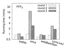
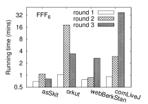
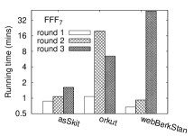
Figure 1: Round-by-round running times of FFF_k on four representative datasets for $k\in[5,7]$.

Round-by-round analysis of FFF_k. In Figure 1 we compare the running times of each round of FFF_k on a selection of benchmarks. Round 1 is typically negligible, regardless of the benchmark and of the value of $k$. Round 2, which computes $2$-paths and small-neighborhoods intersections, is the most expensive step for $k\leq 5$, but its running time can only decrease when $k$ grows (due to the test $|\Gamma^{+}(u)|\geq k-1$ performed by reduce 1 instances, see Algorithm 1). Round 3 becomes more and more expensive as $k$ gets larger, and dominates the running time on webBerkStan and comLiveJ already for $k=6$. This confirms the intuition supported by our theoretical analysis: computing $(k-1)$-cliques on the subgraphs $G^{+}(u)$ induced by high-neighborhoods can be rather time-consuming and becomes the dominant operation as $k$ gets larger. Figure 2a shows the cumulative distribution of $|G^{+}(u)|$, focusing on reduce 3 instances that required more than $100$ ms: notice that a constant fraction of nodes has rather large induced subgraphs (e.g., in egoGplus about 5000 nodes have high neighborhoods with a number of edges in-between $2^{16}$ and $2^{18}$, which is the largest $|G^{+}(u)|$).

(a)

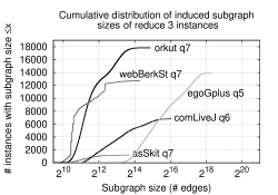
(b)

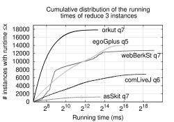
Figure 2: Analysis of reduce instances of round 3 of algorithm FFF_k on a selection of benchmarks.

Scalability on different clusters. Since MapReduce algorithms are inherently parallel, a natural question is how their running times are affected by the cluster size (and ultimately, by the available number of cores). Figure 3 exemplifies the running times on three clusters of 4, 8, and 16 nodes. We focus on FFF_k, which proved to be the algorithm of choice for $k\geq 5$. As an example, the average speedups of FFF₆ when doubling the cluster size from 4 to 8 nodes and from 8 to 16 nodes are 1.44 and 1.53, respectively (the average is taken over the three graph instances). We remark that the maximum theoretical speedup is 2. Similar values can be obtained for the other values of $k$.

While we could not experiment on considerably larger clusters (Amazon AWS limits the number of on-demand instances that can be requested), Figure 2 provides some insights. We focus on round 3, which proved to be the most expensive step when $q_{k}$ is large (see, e.g., webBerkStan and comLiveJ in Figure 1). Figure 2b shows the cumulative distribution of the running times of reduce 3 instances (for executions longer than 100 ms). We focused on the least favorable scenarios, corresponding to large values of $k$ for which the problem is more computationally intensive. The rightmost point on each curve gives the runtime of the slowest reduce instance, that reaches 9 minutes when computing $q_{7}$ on webBerkStan. Although most curves are steeper for short durations, in all cases there are hundreds or even thousands of reduce instances with running times comparable to the slowest one: e.g., in egoGplus more than 2000 reducers are within a factor $8\times$ of the slowest one, and even in the $q_{7}$ computation for webBerkStan 169 instances require more than one minute. This suggests that FFF_k is amenable to further parallelization: we expect that, on a larger cluster, the abundant time-demanding instances could be effectively scheduled to different nodes, yielding globally shorter running times. This analysis is in line with the distribution of induced subgraph sizes observed in Figure 2a, supporting the conclusion that the harmful “curse of the last reducer” phenomenon [35] – where typically 99% of the map/reduce instances terminate quickly, but a very long time could be needed waiting for the last task to succeed – can be kept under control even when $k$ is increased.

6 Approximate counting

In this section we analyze two variants of a sampling strategy that allows us to decrease the overall space usage, starting from the output of map 2 instances. The space saving in map 2 instances propagates to the following phases, reducing the space used by reduce 2 as well as map and reduce 3 instances, and also results in an improved running time (due to reduced local complexities and global work). Instead of performing the sampling directly on the list of edges of the graph, we work by sampling pairs of high-neighbors that are emitted by map 2 instances. If each pair of high-neighbors of a given node $u$ is emitted with probability $p$, then each edge of $G^{+}(u)$ will be included with probability $p$ in the subgraph built by the reduce 3 instance with key $u$; however, the same edge $e$ in two distinct subgraphs $G^{+}(u)$ and $G^{+}(u^{\prime})$ is sampled independently, which results in improved concentration around the mean.

Figure 3: Scalability on different cluster sizes: asSkit, webBerkStan, and comLiveJ (left-to-right).

Plain pair sampling.

We first address the case when pairs of high neighbors are sampled uniformly at random. In details, map 2 instances emit the key-value pair $\langle(x_{i},x_{j});u\rangle$, for all pairs $(x_{i},x_{j})$ with $x_{i}\prec x_{j}$ in $\Gamma^{+}(u)$, with probability $p$, and reduce 3 instances emit the pair $\langle u;q_{u}/p^{(k-1)(k-2)/2}\rangle$. The following results concerning space usage, correctness, and concentration of the estimate around its mean are proved in Appendix B.

Lemma 1.

Let $p\leq 1$ be the edge sampling probability of algorithm FFF_k and let $\alpha$ be a constant in $[0,1)$ such that $1/m^{\alpha}\leq p$. Then algorithm FFF_k  with sampling probability $p$ uses local space $O(mp)$ with high probability.

Theorem 2.

Let $G$ be a graph with $m$ edges and $q_{k}$ $k$-cliques. Let $\widetilde{q_{k}}$ be the estimate returned by algorithm FFF_k with edge sampling probability $p$. For any constant $\varepsilon>0$, there exists a constant $h>0$ such that $|\widetilde{q_{k}}-q_{k}|\leq\varepsilon q_{k}$ with high probability if $p^{(k-1)(k-2)/2}>\frac{hm^{(k-3)/2}\ln m}{\varepsilon^{2}q_{k}}$.

Color-based sampling.

The authors of [28] proposed a sampling technique that allows to increase the expected number of sampled cliques without increasing the number of sampled edges. This is achieved by coloring the nodes of the graph and sampling all monochromatic edges. The same idea can be applied in our setting to sample the emitted pairs in map 2 instances by coloring all nodes in each $\Gamma^{+}(u)$ with $c$ colors and emitting all monochromatic pairs. This has the following implications. Each edge in $G^{+}(u)$ is sampled with probability $1/c$. A $k$-clique $Q_{i}$ with smallest node $u$ is sampled with probability $1/c^{k-2}$, given by the probability of assigning all nodes in $Q_{i}\setminus\{u\}$ with the same color. Hence, reduce 3 instances have to be modified in order to return $\langle u;q_{u}c^{k-2}\rangle$ as partial estimates of the number of $k$-cliques of $G$. Let us call the resulting approximation algorithm cFFF_k.

The analysis of plain pair sampling can be naturally extended to cFFF_k as described in Appendix B. Concentration around the mean is achieved with high probability under the following conditions:

Theorem 3.

Let $G$ be a graph of $m$ edges and $q_{k}$ $k$-cliques. Let $\widetilde{q_{k}}$ be the estimate returned by algorithm cFFF_k with $c$ colors. For any constant $\varepsilon>0$ there exist a constant $h>0$, such that $|\widetilde{q_{k}}-q_{k}|\leq\varepsilon q_{k}$ with high probability if $1/c^{k-2}>\frac{hm^{k-2}\ln m}{\varepsilon^{2}q_{k}}$.

For the case $k=3$, Theorem 3 guarantees (with high probability) concentration around the mean when $1/c\geq(hm\ln m)/(\varepsilon^{2}q_{3})$, which improves the bound in [28], whose worst-case analysis imposes $1/c^{2}\geq(h^{\prime}n^{2}\ln n)/(\varepsilon^{2}q_{3})$ to guarantee concentration on an $n$-node graph.

Discussion. Our estimators fit in the class $\mathcal{MRC}$ as long as $p\leq 1/m^{\alpha}$ (and equivalently $c\geq m^{\alpha}$), for a small constant $\alpha$, as shown by Lemma 1. Moreover, the space reduction translates in improved bounds for the local complexities (in particular for reduce 3 instances that are the most computationally intensive) and work. Notice that the concentration result in Theorem 3 is weaker than that in Theorem 2. However, the color-based sampling strategy increases the expected number of sampled cliques, using sampling probability $p=1/c$, with respect to plain pair sampling. The expected number of sampled cliques shrinks by a factor $p^{(k-1)(k-2)/2}$ for plain sampling, and only by a factor $p^{k-2}$ for color-based sampling. In practice, this boosts the accuracy of the color-based algorithm, which becomes better and better than plain sampling when $k$ grows. We clearly observed this phenomenon, which was also discussed in [28] for triangles, in our experiments.

	cFFF3			cFFF4			cFFF5			cFFF6			cFFF7
	time	sp.	err.	time	sp.	err.	time	sp.	err.	time	sp.	err.	time	sp.	err.
asSkit	2:53	1.12	0.01	2:51	1.15	0.23	2:49	1.17	0.86	2:49	1.15	4.39	2.44	1.54	1.06
orkut	6:08	3.91	0.02	5:52	3.94	0.05	6:09	3.77	0.08	5:57	3.93	0.34	6:30	4.33	2.39
webBerkSt	2:45	1.09	0.05	2:46	1.09	0.16	2:47	1.13	0.17	2:42	1.83	1.22	2:44	18.4	0.39
comLiveJ	3:24	1.62	0.05	3:27	1.57	0.03	3:29	1.78	0.21	3:25	12.11	0.24	3:22	-	-
socLiveJ1	3:42	1.77	0.02	3:40	1.83	0.03	3:31	2.23	0.03	3:36	24.05	0.61	3:41	-	-
egoGplus	4:18	4.03	0.01	4:18	4.16	0.02	4:17	9.11	0.08	4:36	-	-	5:34	-	-

Table 3: Running time, speedup, and approximation quality of cFFF_k for $k\in[3,7]$. The speedup is with respect to FFF_k (see also Table 2) and the error is given as a percentage.

Experiments with approximate counting.

We experimented with both edge-based and color-based sampling, choosing different sampling probabilities and running each algorithm three times on the same instance and platform configuration to increase the statistical confidence of our results. We briefly report on the results obtained by algorithm cFFF_k, whose accuracy in practice outperformed edge sampling. As predicted by the theoretical analysis, sampling is beneficial for round 2, since reduces the number of emitted $2$-paths. In turn, this decreases the number of edges in the induced subgraphs constructed at round 3, yielding substantial benefits on the running time of this round: in particular, in all our tests we observed that the running time of reduce 3 instances of cFFF_k remains almost constant as $k$ increases. Table 3 summarizes the behavior of cFFF_k, showing elapsed time, speedup over the exact algorithm, and accuracy. The experiments were performed on the 16-node cluster using 10 colors, which corresponds to a sampling probability $0.1$. The achieved speedups are dramatic (up to 24$\times$ in socLiveJ1) in all those cases where the exact algorithm took a long time. We were able to compute in a few minutes the estimated number of $q_{6}$ and $q_{7}$ of graphs where the exact computation would have required several hours. The accuracy is very good, especially on the datasets that were most difficult for the exact algorithm: the 24$\times$ faster computation on socLiveJ1, for instance, returned an estimate that was only 0.61% away from the exact value of $q_{6}$.

7 Concluding remarks

We have proposed and analyzed, both theoretically and experimentally, a suite of MapReduce algorithms for counting $k$-cliques in large-scale undirected graphs, for any constant $k\geq 3$. Our experiments, conducted on the Amazon EC2 platform, clearly highlight the algorithm of choice in different scenarios, showing that our algorithms gracefully scale to non-trivial values of $k$, larger instances, and diverse cluster sizes. It is worth noticing that our approach could be slightly modified in order to trade overall space usage for local running time. The actual count of $(k-1)$-cliques at round 3 could be indeed postponed for all nodes $u$ such that $G^{+}(u)$ is too large. In an additional round, map instances would replicate each “uncounted” subgraph $G^{+}(u)$ once per high-neighbor $v$ of $u$, distributing the workload to many reducers. The reduce instance with key $(u,v)$ would thus count the number of $(k-2)$-cliques in its copy of $G^{+}(u)$. This process could be repeated up to $k-4$ times, before copying $\sqrt{m}$ times $G^{+}(u)$ becomes more expensive than counting: each iteration would increase by a factor $\sqrt{m}$ the global space usage and reduce by the same factor the local running times of the reducers, without affecting the total work. We expect this tradeoff to be rather effective on very large clusters, especially for skewed distributions of the high-neighborhoods sizes and large values of $k$, and regard assessing its practicality as an interesting direction.

Appendix A: extended related work

Many related works focus on triangle counting, which is a fundamental algorithmic problem with a variety of applications. For instance, it is closely related to the computation of the clustering coefficient of a graph, which is in turn a widely used measure in the analysis of social networks [22]. Many exact and approximate algorithms tailored to triangles have been developed in the literature in different computational models. The best known sequential counting algorithm is based on fast matrix multiplication [2] and has running time $O(m^{\frac{2\omega}{\omega+1}})$, where $\omega$ is the matrix multiplication exponent: this makes it infeasible even for medium-size graphs. Practical approaches match the $O(m^{3/2})$ bound first achieved in [18] and [12], which is optimal for the listing problem. As shown in [26], many listing algorithms hinge upon a common abstraction that also yields the state-of-the-art sequential implementations for the enumeration of triangles. The input/output complexity of the triangle listing problem is addressed in [27]. Approximate counting algorithms that operate in the data stream model, where the input graph is streamed as a list of edges and the algorithm must compute a solution using small space, are presented in [4, 19, 9, 29, 10], and a randomization technique to speed-up any triangle counting algorithm while keeping a good accuracy is proposed in [36].

A few works have addressed counting problems for subgraphs different from (and more difficult than) triangles. For instance, the techniques in [29] also allow to approximate the number of small cliques, the algorithm from [9] can be extended to any subgraph with 3 or 4 nodes [7], while [23] tackles the problem of counting cycles. All these works focus on graph streams and return estimates, typically concentrated around the true number with high probability. The more general problem of enumerating arbitrary small subgraphs has been also studied in the data stream model [20].

Appendix B: proofs

Tools from the literature

The following property, which is folklore in the triangle counting literature [33], will be crucial in the analysis of our clique estimators (we report its short proof for completeness):

Theorem I.

In a graph with $m$ edges, $|\Gamma^{+}(u)|\leq 2\sqrt{m}$ for each node $u$.

Proof.

Let $h$ be the number of nodes with degree larger than $\sqrt{m}$: since there are $m$ edges, it must be $h\leq 2\sqrt{m}$. If $d(u)>\sqrt{m}$, then nodes in $\Gamma^{+}(u)$ must also have degree larger than $\sqrt{m}$ and their number is upper bounded by $h\leq 2\sqrt{m}$. If $d(u)\leq\sqrt{m}$, the claim trivially holds since $\Gamma^{+}(u)\subseteq\Gamma(u)$. ∎

In the analysis of our approximate estimators we make use of the following (weaker) version of the Chernoff concentration inequality [11]:

Theorem II.

Let $X_{1},\ldots,X_{h}$ be independent identically distributed Bernoulli random variables, with probability of success $p$. Let $X=\sum_{i=1}^{h}X_{i}$ be a random variable with expectation $\mu=p\cdot h$. Then, for any $\varepsilon\in(0,1)$, $Pr\{|X-\mu|>\varepsilon\mu\}\leq 2e^{-\varepsilon^{2}\mu/3}$.

We will also exploit the following conjecture of Paul Erdös, proved in 1970 by Hajnal and Szemeredi [16]:

Theorem III.

Every $n$-node graph with maximum degree $\Delta$ is $(\Delta+1)$-colorable with all color classes of size at least $n/\Delta$.

We say that an event has high probability when it happens, for a graph $G$ of $m$ nodes, with probability at least $1-1/m$, for large enough $m$.

Exact counting

Theorem 1.

Let $G$ be a graph and let $m$ be the number of its edges. Algorithm FFF_k counts the $k$-cliques of $G$ using $O(m^{3/2})$ total space and $O(m^{k/2})$ total work. The local space and the local running time of mappers and reducers are $O(m)$ and $O(m^{(k-1)/2})$, respectively.

Proof.

The total space usage in round 1 is $O(m)$. Map 2 instances produce key-value pairs of constant size, whose total number is upper bounded by $\sum_{u\in V}{{|\Gamma^{+}(u)|}\choose{2}}$, which is at most $2\sqrt{m}\cdot\sum_{u\in V}|\Gamma^{+}(u)|=O(m^{3/2})$ by Theorem I. The data volume can only decrease after the execution of reduce 2 instances and is not affected by round 3. Hence, the total space usage is $O(m^{3/2})$.

We now consider local space. Map 1 instances use constant memory. By Theorem I, the input to any reduce 1 instance has size $O(\sqrt{m})$. Similarly, any map 2 instance receives $O(\sqrt{m})$ input edges and produces $O(m)$ key-value pairs. Consider a reduce 2 instance and let $(x,y)$ be its key. The input of this instance is $\Gamma^{-}(x)\cap\Gamma^{-}(y)\subseteq V$ (without any repetition), and its size is thus $O(n)$. In round 3, map and reduce instances use memory $O(n)$ and $O(m)$, respectively, which concludes the proof of the local space claim (recall that $n\leq 2m$).

By similar arguments, the running time of map instances is $O(1)$, $O(m)$, and $O(n)$, respectively, in the three rounds. Reduce instances require time $O(\sqrt{m})$ and $O(n)$ in rounds 1 and 2, while reduce 3 instances run on graphs of at most $\sqrt{m}$ nodes and require $O(m^{(k-1)/2})$ time. The total work of the algorithm is dominated by the costs of the reducers of the last phase, which is upper bounded by $O(\sum_{u\in V}|\Gamma^{+}(u)|^{k-1})$. By Theorem I, this is $O(m^{(k-2)/2}\sum_{u\in V}|\Gamma^{+}(u)|=O(m^{k/2})$.

Each clique is counted exactly once by the reducer associated to its minimum node (according to $\prec$), proving the correctness of the algorithm. ∎

Approximate counting

We now prove the results about space usage, correctness, and concentration of the plain pair sampling algorithm described in Section 6. Let $\mathcal{Q}=\{Q_{1},\ldots,Q_{q_{k}}\}$ be the set of $k$-cliques of $G$. Let $Q_{i}\in\mathcal{Q}$ be a clique and let $u$ be its smallest node (according to $\prec$). We say that $Q_{i}$ is sampled if all pairs in $Q_{i}\setminus\{u\}$ were emitted by the map 2 instance with key $u$.

Lemma 1.

Let $p\leq 1$ be the edge sampling probability of algorithm FFF_k and let $\alpha$ be a constant in $[0,1)$ such that $1/m^{\alpha}\leq p$. Then algorithm FFF_k  with sampling probability $p$ uses local space $O(mp)$ with high probability.

Proof.

We will prove the claim for reduce 3 instances; similar arguments can be used to prove the bounds for reduce 2 and map 3 instances, recalling that $n\leq 2m$.

By Theorem I each subgraph $G^{+}(u)$ has at most $2\sqrt{m}$ nodes. Since the reduce 3 instance with key $u$ receives an edge $(x,y)\in G^{+}(u)$ if and only if the map 2 instance with key $u$ sampled the pair $(x,y)$ (event that has probability $p$), we have that the expected input size of any reduce 2 instance is at most $2pm$.

Being each pair of high-neighbors of a node $u$ sampled independently by all the other, a simple application of the Chernoff bound allows to prove that the probability of one reduce 3 instance to receive more than $4pm$ values is less than $e^{-2pm/3}$, and a union bound gives that the probability of any of the reduce 3 instances to receive more than $4pm$ values is bounded by $n/e^{2pm/3}$. Since $p\geq 1/m^{\alpha}$, for large enough $m$ this probability is smaller than $1/m$, which concludes the proof. ∎

Claim 1.

Algorithm FFF_k with edge sampling returns an estimate $\widetilde{q_{k}}$ with expected value $E[\widetilde{q_{k}}]=q_{k}$, where $q_{k}$ is the number of $k$-cliques in the input graph $G$.

Proof.

Let $Q_{i}\in\mathcal{Q}$ be a clique in $G$ and let $u$ be its smallest node (according to $\prec$). Clique $Q_{i}$ contributes to the estimate of the number of cliques in $G$ if the map 2 instance handling input $\langle u;\Gamma^{+}(u)\rangle$ emits all pairs of nodes in $Q_{i}\setminus{u}$, i.e., if it is sampled. Let $X_{i}$ be the random variable indicating the event “the clique $Q_{i}$ is sampled”. Since each pair is sampled by the algorithm independently with probability $p$ and there are ${k-1}\choose 2$ distinct (unordered) pairs in a set of $k-1$ elements, $Pr\{X_{i}=1\}=p^{(k-1)(k-2)/2}$, hence $E[X_{i}]=p^{(k-1)(k-2)/2}$. Now we can define $X=\sum_{i=1}^{q_{k}}X_{i}$, and by linearity of expectation we have that $E[X]=q_{k}p^{(k-1)(k-2)/2}$. Since $\widetilde{q_{k}}=X/p^{(k-1)(k-2)/2}$ the claim follows. ∎

Theorem 2.

Let $G$ be a graph with $m$ edges and $q_{k}$ $k$-cliques. Let $\widetilde{q_{k}}$ be the estimate returned by algorithm FFF_k with edge sampling probability $p$. For any constant $\varepsilon>0$, there exists a constant $h>0$ such that $|\widetilde{q_{k}}-q_{k}|\leq\varepsilon q_{k}$ with high probability if $p^{(k-1)(k-2)/2}>\frac{hm^{(k-3)/2}\ln m}{\varepsilon^{2}q_{k}}$.

Proof.

We proved that the expected value of $\widetilde{q_{k}}$ is $q_{k}$ in Claim 1; we will now deal with the concentration of $\widetilde{q_{k}}$ around its mean. Let $H$ be the graph defined as follows:

• The node set of $H$ is the set of $k$-cliques $\mathcal{Q}$ of $G$.

• Let $Q_{i}$ and $Q_{j}$ be two $k$-cliques with the same smallest node $u$: there is an edge between $Q_{i}$ and $Q_{j}$ in $H$ if and only if $Q_{i}\setminus\{u\}$ and $Q_{j}\setminus\{u\}$ have at least one common edge.

Cliques that are adjacent in $H$ must thus share at least three of their $k$ nodes, including the smallest node. Considering that graphs $G^{+}(u)$ have at most $\sqrt{m}$ nodes, we have that the maximum degree of a node in $H$ is therefore $O(m^{(k-3)/2})$.

Theorem III by Hajnal and Szemeredi implies that there exists a node coloring of $H$, using $C\in O(m^{(k-3)/2})$ colors, such that each monochromatic set of nodes has size $\Theta(q_{k}/m^{(k-3)/2})$, since $H$ has $q_{k}$ nodes.

For each $j\in[1,q_{k}]$, let $X_{j}$ be the indicator variable that is 1 when $Q_{j}$ is sampled. Let $S_{1},\ldots,S_{C}$ be the sets of monochromatic nodes in $H$ and, for each $i\in[1,C]$, let

$$X_{S_{i}}=\sum_{j:Q_{j}\in S_{i}}X_{j}$$ (1)

The terms of $X_{S_{i}}$ are independent. Hence, we can apply to $X_{S_{i}}$ the Chernoff bound as in Theorem II obtaining:

$$Pr\{|X_{S_{i}}-\mu_{i}|>\varepsilon\mu_{i}\}\leq 2e^{-\mu_{i}\varepsilon^{2}/3}\,.$$

where $\mu_{i}=E[X_{S_{i}}]$. By Equation 1, for each set $S_{i}$ we have:

$$\mu_{i}\in\Theta\left(\frac{p^{(k-1)(k-2)/2}q_{k}}{m^{(k-3)/2}}\right)$$

since $E[X_{j}]=p^{(k-1)(k-2)/2}$, as shown in the proof of Claim 1. By the same proof, $\mu=\sum_{i=1}^{C}\mu_{i}=p^{(k-1)(k-2)/2}q_{k}$.

If we define $X=\sum_{i=1}^{C}X_{S_{i}}$ and we apply the union bound we can conclude that

$$Pr\{|X-\mu|>\varepsilon\mu\}\leq c_{1}m^{\frac{k-3}{2}}e^{-\frac{c_{2}\varepsilon^{2}q_{k}p^{(k-1)(k-2)/2}}{m^{(k-3)/2}}}$$

by appropriately choosing constants $c_{1}$ and $c_{2}$. By imposing

$$c_{1}m^{\frac{k-3}{2}}e^{-\frac{c_{2}\varepsilon^{2}q_{k}p^{(k-1)(k-2)/2}}{m^{(k-3)/2}}}\leq\frac{1}{m}$$

the claim follows with standard algebraic calculations. ∎

The analysis above can be naturally extended to algorithm cFFF_k. Lemma 1 holds for algorithm cFFF_k just by using $p=1/c$. The estimate returned by algorithm cFFF_k has expected value $q_{k}$, and this can be proved using arguments similar to those in the proof of Claim 1. The arguments of the proof of Theorem 2 can also be used to prove concentration around the mean for algorithm cFFF_k, considering that correlation of sampled $k$-cliques arises as soon as the cliques share a node besides the minimum node, instead of an edge. Hence, concentration is achieved with high probability under the conditions expressed by Theorem 3.

We observed in Section 6 that, for $k=3$, our concentration results require weaker conditions than the triangle counting algorithm from [28]. This is due to the fact that we color the same node $x\in\Gamma^{+}(u)\cap\Gamma^{+}(v)$ independently for $u$ and $v$, which allows us to reduce the maximum degree of the interference graph $H$ in the application of the Hajnal-Szemeredi theorem.

Appendix C: detailed benchmark statistics and number of cliques

	$n$ ($=q_{1}$)	$m$ ($=q_{2}$)	$q_{3}$	$q_{4}$	$q_{5}$	$q_{6}$	$q_{7}$
citPat	3 774 768	16 518 947	7 515 023	3 501 071	3 039 636	3 151 595	1 874 488
(264.0 MB)		($4.38\times$)	($0.45\times$)	($0.47\times$)	($0.87\times$)	($1.04\times$)	($0.6\times$)
youTube	1 134 890	2 987 624	3 056 386	4 986 965	7 211 947	8 443 803	7 959 704
(38.7 MB)		($2.63\times$)	($1.02\times$)	($1.63\times$)	($1.44\times$)	($1.17\times$)	($0.94\times$)
locGowalla	196 591	950 327	2 273 138	6 086 852	14 570 875	28 928 240	47 630 720
(11.1 MB)		($4.83\times$)	($2.39\times$)	($2.67\times$)	($2.39\times$)	($1.98\times$)	($1.65\times$)
socPokec	1 632 803	22 301 964	32 557 458	42 947 031	52 831 618	65 281 896	83 896 509
(309.1 MB)		($13.65\times$)	($1.46\times$)	($1.32\times$)	($1.23\times$)	($1.18\times$)	($1.28\times$)
webGoogle	875 713	4 322 051	13 391 903	39 881 472	105 110 267	252 967 829	605 470 026
(59.5 MB)		($4.93\times$)	($3.1\times$)	($2.98\times$)	($2.63\times$)	($2.40\times$)	($2.39\times$)
webStan	281 903	1 992 636	11 329 473	78 757 781	620 210 972	4 859 571 082	34 690 796 481
(26.4 MB)		($7.07\times$)	($5.68\times$)	($6.95\times$)	($7.87\times$)	($7.83\times$)	($7.13\times$)
asSkit	1 696 415	11 095 298	28 769 868	148 834 439	1 183 885 507	9 759 000 981	73 142 566 591
(149.1 MB)		($6.54\times$)	($2.59\times$)	($5.17\times$)	($7.95\times$)	($8.24\times$)	($7.49\times$)
orkut	3 072 441	117 185 083	627 584 181	3 221 946 137	15 766 607 860	75 249 427 585	353 962 921 685
(1 687.8 MB)		($38.14\times$)	($5.35\times$)	($5.13\times$)	($4.89\times$)	($4.77\times$)	($4.70\times$)
webBerkStan	685 230	6 649 470	64 690 980	1 065 796 916	21 870 178 738	460 155 286 971	9 398 610 960 254
(89.4 MB)		($9.70\times$)	($9.73\times$)	($16.48\times$)	($20.52\times$)	($21.04\times$)	($20.42\times$)
comLiveJ	3 997 962	34 681 189	177 820 130	5 216 918 441	246 378 629 120	10 990 740 312 954	445 377 238 737 777
(501.6 MB)		($8.67\times$)	($5.12\times$)	($29.34\times$)	($47.22\times$)	($44.6\times$)	(40.52$\times$)
socLiveJ1	4 847 571	42 851 237	285 730 264	9 933 532 019	467 429 836 174	20 703 476 954 640	849 206 163 678 934
(627.7 MB)		($8.84\times$)	($6.67\times$)	($34.7\times$)	($47.05\times$)	($44.29\times$)	(41.01$\times$)
egoGplus	107 614	12 238 285	1 073 677 742	78 398 980 887	4 727 009 242 306	242 781 609 271 577	11 381 161 386 691 540
(538.5 MB)		($113.72\times$)	($87.73\times$)	($73.01\times$)	($60.29\times$)	(51.36$\times$)	(46.87$\times$)

Benchmark statistics: number $n$ of nodes, number $m$ of edges, numbers of cliques on $3$, $4$, $5$, $6$, and $7$ nodes (clique numbers in italic are approximations obtained by our color-based sampling algorithm, using 10 colors). Benchmarks are sorted by increasing $q_{7}$. For each benchmark, we also report in parentheses the storage in MB with no compression and the ratio $q_{k+1}/q_{k}$ (which is half the average node degree for $k=1$). Notice the large values of these ratios for benchmarks socLiveJ1, comLiveJ, webBerkStan, and egoGplus.

References

- [1] F. N. Afrati, D. Fotakis, and J. D. Ullman. Enumerating subgraph instances using map-reduce. In C. S. Jensen, C. M. Jermaine, and X. Zhou, editors, ICDE, pages 62–73. IEEE Computer Society, 2013.
- [2] N. Alon, R. Yuster, and U. Zwick. Finding and counting given length cycles. Algorithmica, 17(3):209–223, 1997.
- [3] Apache Hadoop. http://hadoop.apache.org/.
- [4] Z. Bar-Yossef, R. Kumar, and D. Sivakumar. Reductions in streaming algorithms, with an application to counting triangles in graphs. In Proceedings of the thirteenth annual ACM-SIAM symposium on Discrete algorithms, pages 623–632. Society for Industrial and Applied Mathematics, 2002.
- [5] A. Barabási and R. Albert. Emergence of scaling in random networks. Science, 286(5439):509–512, 1999.
- [6] L. Becchetti, C. Castillo, D. Donato, S. Leonardi, and R. A. Baeza-Yates. Link-based characterization and detection of web spam. In AIRWeb, pages 1–8, 2006.
- [7] I. Bordino, D. Donato, A. Gionis, and S. Leonardi. Mining large networks with subgraph counting. In Data Mining, 2008. ICDM’08. Eighth IEEE International Conference on, pages 737–742. IEEE, 2008.
- [8] S. Borgatti, M. Everett, and L. Freeman. UCINET for Windows: Software for Social Network Analysis. Harvard, MA: Analytic Technologies, 2002.
- [9] L. S. Buriol, G. Frahling, S. Leonardi, A. Marchetti-Spaccamela, and C. Sohler. Counting triangles in data streams. In Proceedings of the twenty-fifth ACM SIGMOD-SIGACT-SIGART symposium on Principles of database systems, pages 253–262. ACM, 2006.
- [10] L. S. Buriol, G. Frahling, S. Leonardi, and C. Sohler. Estimating clustering indexes in data streams. In Algorithms–ESA 2007, pages 618–632. Springer, 2007.
- [11] H. Chernoff. A note on an inequality involving the normal distribution. Annals of Probability, 9(3):533–535, 1981.
- [12] N. Chiba and T. Nishizeki. Arboricity and subgraph listing algorithms. SIAM J. Comput., 14(1):210–223, 1985.
- [13] J. Dean and S. Ghemawat. Mapreduce: Simplified data processing on large clusters. In Proc. 6th Conf. on Symposium on Operating Systems Design & Implementation (OSDI’04), pages 10–10, 2004.
- [14] D. Gibson, R. Kumar, and A. Tomkins. Discovering large dense subgraphs in massive graphs. In Proceedings of the 31st international conference on Very large data bases, pages 721–732. VLDB Endowment, 2005.
- [15] M. T. Goodrich, N. Sitchinava, and Q. Zhang. Sorting, searching, and simulation in the mapreduce framework. In Proc. 22nd Int. Conf. on Algorithms and Computation, ISAAC’11, pages 374–383, 2011.
- [16] A. Hajnal and E. Szemerédi. Proof of a conjecture of Erdös. Combinatorial Theory and Its Applications, 2:601–623, 1970.
- [17] R. A. Hanneman and M. Riddle. Introduction to social network methods. University of California, Riverside, Riverside, CA, 2005.
- [18] A. Itai and M. Rodeh. Finding a minimum circuit in a graph. SIAM J. Comput., 7(4):413–423, 1978.
- [19] H. Jowhari and M. Ghodsi. New streaming algorithms for counting triangles in graphs. In Computing and Combinatorics, pages 710–716. Springer, 2005.
- [20] D. M. Kane, K. Mehlhorn, T. Sauerwald, and H. Sun. Counting arbitrary subgraphs in data streams. In Proc. 39th Int. Colloquium on Automata, Languages and Programming (ICALP 2012), volume 7392 of LNCS, pages 598–609, 2012.
- [21] H. Karloff, S. Suri, and S. Vassilvitskii. A model of computation for MapReduce. In Proc. Twenty-First Annual ACM-SIAM Symposium on Discrete Algorithms, SODA ’10, pages 938–948, 2010.
- [22] M. N. Kolountzakis, G. L. Miller, R. Peng, and C. E. Tsourakakis. Efficient triangle counting in large graphs via degree-based vertex partitioning. Internet Mathematics, 8(1-2):161–185, 2012.
- [23] M. Manjunath, K. Mehlhorn, K. Panagiotou, and H. Sun. Approximate counting of cycles in streams. In Algorithms–ESA 2011, pages 677–688. Springer, 2011.
- [24] R. Milo, S. Shen-Orr, S. Itzkovitz, N. Kashtan, D. Chklovskii, and U. Alon. Network motifs: simple building blocks of complex networks. Science, 298(5594):824–827, 2002.
- [25] S. Muthukrishnan. Data streams: Algorithms and applications. Foundations and Trends in Theoretical Computer Science, 1(2), 2005.
- [26] M. Ortmann and U. Brandes. Triangle listing algorithms: Back from the diversion. In C. C. McGeoch and U. Meyer, editors, ALENEX, pages 1–8. SIAM, 2014.
- [27] R. Pagh and F. Silvestri. The input/output complexity of triangle enumeration. In Proc. 33rd ACM SIGMOD-SIGACT-SIGART Symposium on Principles of Database Systems, PODS ’14, pages 224–233. ACM, 2014.
- [28] R. Pagh and C. E. Tsourakakis. Colorful triangle counting and a mapreduce implementation. Inf. Process. Lett., 112(7):277–281, 2012.
- [29] A. Pavan, K. Tangwongsan, S. Tirthapura, and K.-L. Wu. Counting and sampling triangles from a graph stream. PVLDB, 6(14):1870–1881, 2013.
- [30] A. Pietracaprina, G. Pucci, M. Riondato, F. Silvestri, and E. Upfal. Space-round tradeoffs for mapreduce computations. In Proc. 26th ACM Int. Conf. on Supercomputing (ICS’12), pages 235–244, 2012.
- [31] A. Rajaraman and J. D. Ullman. Mining of Massive Datasets. Cambridge University Press, 2012.
- [32] B. Saha, A. Hoch, S. Khuller, L. Raschid, and X.-N. Zhang. Dense subgraphs with restrictions and applications to gene annotation graphs. In Research in Computational Molecular Biology, pages 456–472. Springer, 2010.
- [33] T. Schank and D. Wagner. Approximating clustering coefficient and transitivity. J. Graph Algorithms Appl., 9(2):265–275, 2005.
- [34] SNAP graph library. http://snap.stanford.edu/.
- [35] S. Suri and S. Vassilvitskii. Counting triangles and the curse of the last reducer. In Proc. 20th International Conference on World Wide Web, WWW ’11, pages 607–614, 2011.
- [36] C. E. Tsourakakis, U. Kang, G. L. Miller, and C. Faloutsos. DOULION: Counting triangles in massive graphs with a coin. In Proc. 15th ACM SIGKDD Int. Conf. on Knowledge Discovery and Data Mining (KDD’09), pages 837–846, 2009.
- [37] J. S. Vitter. Algorithms and data structures for external memory. Found. Trends Theor. Comput. Sci., 2(4):305–474, 2008.