Existence and stability properties of entire solutions to the polyharmonic equation $(-\Delta)^{m}u=e^{u}$ for any $m\geq 1$

Abstract.

We study existence and stability properties of entire solutions of a polyharmonic equation with an exponential nonlinearity. We study existence of radial entire solutions and we provide some asymptotic estimates on their behavior at infinity. As a first result on stability we prove that stable solutions (not necessarily radial) in dimensions lower than the conformal one never exist. On the other hand, we prove that radial entire solutions which are stable outside a compact always exist both in high and low dimensions. In order to prove stability of solutions outside a compact set we prove some new Hardy-Rellich type inequalities in low dimensions.

1. Introduction

We are interested in existence, nonexistence and stability properties of global solutions for the polyharmonic equation

(1) $$(-\Delta)^{m}u=e^{u}\qquad\text{in }\mathbb{R}^{n}\,.$$

This problem is the natural extension to the polyharmonic case of the Gelfand equation [24]

(2) $$-\Delta u=e^{u}\quad\mbox{in}\quad\mathbb{R}^{n},\qquad n\geq 1\,.$$

Equation (2) describes problems of thermal self-ignition [24], diffusion phenomena induced by nonlinear sources [27] or a ball of isothermal gas in gravitational equilibrium as proposed by lord Kelvin [9]. For results concerning properties of solutions of the Gelfand equation in the whole $\mathbb{R}^{n}$ or in bounded domains see [5, 11, 17, 26, 33] and the references therein.

Recently, problem (1) in the biharmonic case $m=2$ was widely studied, see [3, 4, 6, 7, 10, 13, 14, 16, 30, 37, 38]. In the listed papers the biharmonic version of the Gelfand equation was considered both in bounded domains with suitable boundary conditions and in the whole $\mathbb{R}^{n}$; several questions were tackled, from the existence of solutions to their qualitative and stability properties. For other results concerning radial entire solutions of nonlinear biharmonic equations see also [18, 19, 20, 22, 23, 28] and the references therein.

The study of higher order elliptic equations like in (1) is motivated by the problem formulated by P.L. Lions [25, Section 4.2 (c)], namely: Is it possible to obtain a description of the solution set for higher order semilinear equations associated to exponential nonlinearities?

Our paper is essentially focused on the existence and stability properties of entire solutions of (1). This paper has the purpose of being a first step in a deeper comprehension of properties of entire solutions of (1). Throughout this paper, by entire solution to problem (1) we mean a classical solution $u$ of the equation in (1) which exists for all $x\in\mathbb{R}^{n}$.

Concerning existence of entire solutions we describe in which way existence of global radial solutions of (1) is influenced by the fact that $m$ is even or not. For results about radial solutions of nonlinear polyharmonic equations see the papers [15, 29] and the references therein.

In the present paper, in looking for radial solutions of (1), we consider the following initial value problem

(3) $$\left\{\begin{array}[]{ll}(-\Delta)^{m}u(r)=e^{u(r)}\qquad\text{for }r\in[0,R(\alpha_{0},\dots,\alpha_{m-1}))\\ u(0)=\alpha_{0}\,,\quad u^{\prime}(0)=0\\ \Delta^{k}u(0)=\alpha_{k}\,,\quad(\Delta^{k}u)^{\prime}(0)=0\,\quad\text{for any }k\in\{1,\dots,m-1\}\end{array}\right.$$

where $\alpha_{0},\dots,\alpha_{m-1}$ are arbitrary real numbers and $R(\alpha_{0},\dots,\alpha_{m-1})$ is the supremum of the maximal interval of continuation of the corresponding solution. The conditions $u^{\prime}(0)=0$ and on $(\Delta^{k}u)^{\prime}(0)=0$ are necessary for having smoothness of the solution at the origin.

As a first result, we prove that in the case $m$ odd, for any $\alpha_{0},\dots,\alpha_{m-1}$ the corresponding solution of (3) is an entire solution of (1), see Theorem 2.1. In dimension $n=1$ we also prove that all solutions of (1), not necessarily symmetric, are global, see Theorem 2.4.

On the other hand, if $m$ is even and $n=1$ or $n=2$ then any solution of (3) is not global whereas in dimension $n\geq 3$ both existence and nonexistence of global solutions may occur. In this last situation we give a sufficient and necessary condition for the existence of radial entire solutions of (1), see Theorem 2.2. More precisely, this theorem shows that for any $\alpha_{0}\in\mathbb{R}$, (3) admits a global solution if and only if the $(m-1)$-tuple $(\alpha_{1},\dots,\alpha_{m-1})$ belongs to a suitable nonempty closed set depending on $\alpha_{0}$, denoted by $\mathcal{A}_{\alpha_{0}}$. The nonexistence result in Theorem 2.2 (i) is extended for $n=1$ to all solutions of (1), see Theorem 2.3.

The second purpose of this paper is to shed some light on the asymptotic behavior of global solutions of (3) as $r\to+\infty$ and on their stability properties.

In this direction we first show in Proposition 2.1 that all entire solutions of (1) are unbounded from below. In Theorem 2.5 we restrict out attention to radial solutions of (1). When $m$ is odd we prove that for some special values of the initial conditions, problem (3) admits solutions which blow down to $-\infty$ at least as $r^{4}$ as $r\to+\infty$. Moreover if $1\leq n\leq 2m-1$ all radial solutions of (1) blow down to $-\infty$ at least as a positive and integer power of $r$.

On the other hand when $m$ is even we prove that for any $\alpha_{0}\in\mathbb{R}$, solutions corresponding to initial conditions satisfying $(\alpha_{1},\dots,\alpha_{m-1})\in\displaystyle{\mathop{\mathcal{A}_{\alpha_{0}}}^{\circ}}$, behave like $-Cr^{2m-2}$ as $r\to+\infty$ for a suitable constant $C>0$. If $(\alpha_{1},\dots,\alpha_{m-1})\in\partial\mathcal{A}_{\alpha_{0}}$ then the corresponding solution $u$ satisfies $u(r)=o(r^{2m-2})$ as $r\to+\infty$; however we are able to prove that $u$ blows down to $-\infty$ at least as a logarithm as $r\to+\infty$, see Theorem 2.5 (iv). Such a logarithmic behavior actually occurs when $m=2$ and $n\geq 5$, see [3]. When $m\geq 3$ is any integer (possibly also odd) and $n=2m$ a logarithmic behavior can be observed for a special class of solutions of (1), see [32] and the references therein. More precisely, combining Theorems 1-2 in [32], it can be shown that among solutions of (1) satisfying the condition $\int_{\mathbb{R}^{2m}}e^{u}<+\infty$, the only ones which show a logarithmic behavior at infinity are the explicit solutions given by

(4) $$u(x)=2m\log\frac{2[(2m)!]^{\frac{1}{2m}}\lambda}{1+\lambda^{2}|x-x_{0}|^{2}}$$

where $\lambda>0$ and $x_{0}\in\mathbb{R}^{2m}$. For more details see also Proposition 2.2 and Corollary 2.1 in the present paper.

Then we focus our attention on stability and stability outside a compact set. For a rigorous definition of these two notions see Section 3. In Theorem 3.1 we prove that (1) admits no stable solutions (also non radial) if $n$ is less or equal than the conformal dimension $2m$. However, in Theorems 3.4-3.5 we are able to prove that if $3\leq n\leq 2m$ then (1) admits radial solutions which are stable outside a compact set. Moreover if $m\geq 3$ is odd and $1\leq n\leq 2m-1$ then all radial solutions of (1) are stable outside a compact set, see Theorem 3.3.

In the supercritical dimensions $n>2m$ we prove that if $m$ is odd then (1) admits radial solutions that are stable outside a compact set and if $m$ is even then, for any $\alpha_{0}\in\mathbb{R}$, all solutions of (3) such that $(\alpha_{1},\dots,\alpha_{m-1})\in\displaystyle{\mathop{\mathcal{A}_{\alpha_{0}}}^{\circ}}$, are stable outside a compact set; the question about the stability outside a compact set in the case $(\alpha_{1},\dots,\alpha_{m-1})\in\partial\mathcal{A}_{\alpha_{0}}$ is still open, see Problem 3.1 (ii).

The question about the existence of (globally) stable solutions is completely open both in the cases $m$ odd and $m$ even, see Problem 3.1 (iii). Let us try to explain the main difficulties that one has to face in order to determine stability of radial solutions. In the case $m=1$ a complete description of stability and stability outside compact sets of solutions (also non radial) of (1) is available, see [11, 17]. In the case $m=2$ a complete picture on stability and stability outside compact sets was given in [6, 16] at least for radial solutions.

If we look at radial solutions in the case $m=2$, we see that in [6] the authors are able to obtain asymptotic and global estimates on solutions by exploiting a suitable change of variables which reduces the ordinary differential equation in (3) into a nonlinear fourth order autonomous equation, see [6, Proof of Lemma 12]. In turn, this fourth order autonomous equation may reduced to a dynamical system of four first order equations. In this situation the dimension $n$ plays a crucial role in determining stability properties of radial solutions: indeed in dimension $n\geq 13$ the above mentioned fourth order autonomous equation shows a non oscillatory behavior of its solutions and this, combined with the classical Hardy-Rellich inequality [36], gives stability of solutions; on the other hand in dimensions $5\leq n<13$ ($n=4$ is the critical dimension) the autonomous fourth order equation shows an oscillatory behavior and this justifies the existence of radial unstable solutions.

When we consider higher powers $m$ of $-\Delta$ the situation seems to be quite different for the following reason. In a completely similar way the ordinary differential equation in (3) may be reduced to an autonomous equation of order $2m$. But this time a non oscillatory behavior, similar to the one observed in the case $m=2$ when $n\geq 13$, seems not to take place also in large dimensions as one can see from Section 11.

A relevant part of this paper is devoted to a class of Hardy-Rellich type inequalities when $n$ is less or equal than the corresponding critical dimension. The first result in this direction is Proposition 4.2 which can be obtained with an iterative procedure by using a result of [8]. The results in Theorems 4.1-4.2 are new and their proofs are based on suitable Emden type transformation. This kind of procedure was already used in [8] in order to obtain Hardy-Rellich type inequalities in conical domains.

This paper is organized as follows. In Section 2 we state existence and nonexistence results for solutions to (1) and we provide some estimates on the asymptotic behavior of its radial solutions as $|x|\to+\infty$. In Section 3 we give some results about stability and stability outside compact sets of solutions to (1). To this end, we need some Hardy-Rellich inequalities which are stated in Section 4. Sections 5-10 are devoted to the proofs of the main results. In Section 11 we explain in which way further results on radial solutions of (1) could be obtained by mean of a suitable change of variable and we present some open questions. Finally in the appendix we state a couple of well-known results dealing with continuous dependence on the initial data and with a comparison principle.

2. Existence and asymptotic behavior of radial entire solutions of (1)

We start with following existence result for radial entire solutions of (1) in the case $m$ odd :

Theorem 2.1.

Let $n\geq 1$ and $m\geq 1$ odd. Then for any $\alpha_{0},\dots,\alpha_{m-1}\in\mathbb{R}$ problem (3) admits a unique global solution.

In order to describe what happens in the case $m$ even we introduce the following notation accordingly with [4, 6]: we write $\alpha$ in place of $\alpha_{0}\in\mathbb{R}$ and we rename the numbers $\alpha_{1},\dots,\alpha_{m-1}$ respectively $\beta_{1},\dots,\beta_{m-1}$. Then we put $\beta:=(\beta_{1},\dots,\beta_{m-1})\in\mathbb{R}^{m-1}$ and we denote by $u_{\alpha,\beta}$ the corresponding solution of (3). Finally for any $\alpha\in\mathbb{R}$ fixed, we introduce the set

(5) $$\mathcal{A}_{\alpha}:=\{\beta\in\mathbb{R}^{m-1}:u_{\alpha,\beta}\ \text{is a global solution of }\eqref{Cauchy}\}\,.$$

We prove

Theorem 2.2.

Let $m\geq 2$ even and let $\mathcal{A}_{\alpha}$ be the set introduced in (5). Then the following statements hold true:

• if $n=1$ or $n=2$ then for any $\alpha\in\mathbb{R}$ the set $\mathcal{A}_{\alpha}$ is empty.

• if $n\geq 3$ then for any $\alpha\in\mathbb{R}$ the set $\mathcal{A}_{\alpha}$ is nonempty and moreover there exists a function

  $\Phi_{\alpha}:\mathbb{R}^{m-2}\to(-\infty,0)$ such that

  $$\mathcal{A}_{\alpha}=\{\beta=(\beta_{1},\dots,\beta_{m-1})\in\mathbb{R}^{m-1}:\beta_{m-1}\leq\Phi(\beta_{1},\dots,\beta_{m-2})\}\,;$$

• if $n\geq 3$ then for any $\alpha\in\mathbb{R}$, $\Phi_{\alpha}$ is a continuous function, $\mathcal{A}_{\alpha}$ is closed, $\partial\mathcal{A}_{\alpha}$ coincides with the graph of $\Phi_{\alpha}$ and

  $${\mathop{\mathcal{A}_{\alpha}}^{\circ}}=\{\beta=(\beta_{1},\dots,\beta_{m-1})\in\mathbb{R}^{m-1}:\beta_{m-1}<\Phi(\beta_{1},\dots,\beta_{m-2})\}\,;$$

• if $n\geq 3$ and $m\geq 4$ then for any $\alpha\in\mathbb{R}$, $\Phi_{\alpha}$ is decreasing with respect to each variable i.e. the map $t\mapsto\Phi_{\alpha}(\beta_{1},\dots,\beta_{k-1},t,\beta_{k+1},\dots,\beta_{m-2})$ is decreasing in $\mathbb{R}$ for any $k\in\{1,\dots,m-2\}$.

When $m=2$ the function $\Phi_{\alpha}$ introduced in the statement of Theorem 2.2 is defined on the zero dimensional space $\{0\}$ and the set $\mathcal{A}_{\alpha}$ becomes $\{\beta\in\mathbb{R}:\beta\leq\Phi_{\alpha}(0)\}$. The result in this particular case was already obtained in [3].

We observe that the nonexistence result proved in Theorem 2.2 for $n=1$ remains valid also for any kind of solutions of (1), also nonsymmetric:

Theorem 2.3.

If $n=1$ and $m\geq 2$ is even then (1) admits no entire solutions.

On the other hand, when $n=1$ and $m\geq 1$ is odd we have

Theorem 2.4.

Let $n=1$ and $m\geq 1$ odd. Then any local solution of the ordinary differential equation corresponding to (1), is global. Moreover if $m=1$ then any solution of (1) is symmetric with respect to some point $x_{0}\in\mathbb{R}$. On the other hand if $m\geq 3$, (1) admits solutions which are not symmetric with respect to any point $x_{0}\in\mathbb{R}$.

Next we provide some information on the qualitative behavior of entire solutions of (1). First we show that any entire solution (possibly non radial) of (1) is not bounded from below. Indeed if $u$ is a solution to (1) such that $u\geq M$ for some $M\in\mathbb{R}$ then for any $q>1$ there exists $K(M,q)>0$ such that the inequality

$$(-\Delta)^{m}u\geq K(M)|u|^{q}\quad\text{in }\mathbb{R}^{n}\,$$

holds true. Then, from [35, Theorem 4.1], we infer

Proposition 2.1.

For any $n\geq 1$ and $m\geq 1$, problem $(\ref{eq_1})$ admits no entire solutions bounded from below.

Then we deal with the asymptotic behavior of radial entire solutions of (1) as $|x|\to+\infty$. We prove

Theorem 2.5.

Let $n\geq 1$. Then the following statements hold true:

• if $m\geq 3$ is odd then for any solution $u$ of (3) satisfying ${\rm sign}\,\alpha_{k}\neq(-1)^{k}$ for at least one value of $k\in\{1,\dots,m-1\}$, we have

  (6) $$u(r)<-Cr^{4}\qquad\text{for any }r>\overline{r}$$

  for some $C,\overline{r}>0$;

• if $m\geq 3$ is odd and $1\leq n\leq 2m-1$ then any solution $u$ of (3) satisfies

  $$u(r)<-Cr^{K}\qquad\text{for any }r>\overline{r}$$

  for some $C,\overline{r}>0$ and $K$ positive integer;

• if $n=1$ and $m\geq 1$ is odd then any solution $u$ of (1) (also nonsymmetric) satisfies

  $$u(x)<-C|x|^{K}\qquad\text{for any }|x|>\overline{r}$$

  for some $C,\overline{r}>0$ and $K$ positive integer;

• if $m\geq 2$ is even, $\alpha\in\mathbb{R}$ and $\beta\in\displaystyle{\mathop{\mathcal{A}_{\alpha}}^{\circ}}$ then there exists $C>0$ such that

  $$u_{\alpha,\beta}(r)\sim-Cr^{2m-2}\qquad\text{as }r\to+\infty$$

  where we denoted by $u_{\alpha,\beta}$ the unique solution of (3) corresponding to the couple $(\alpha,\beta)\in\mathbb{R}^{m}$.

• if $m\geq 2$ is even, $\alpha\in\mathbb{R}$ and $\beta\in\partial\mathcal{A}_{\alpha}$ then

  $$u_{\alpha,\beta}(r)=o(r^{2m-2})\qquad\text{as }r\to+\infty$$

  and there exist $C,\overline{r}>0$ such that

  $$u_{\alpha,\beta}(r)<-2m\log r+C\qquad\text{for any }r>\overline{r}$$

  where we denoted by $u_{\alpha,\beta}$ the unique solution of (3) corresponding to the couple $(\alpha,\beta)\in\mathbb{R}^{m}$.

Problem 2.1.

As possible improvements of Theorem 2.5 we suggest the following open questions:

• let $m\geq 3$ odd. Provide an upper estimate for all radial solutions of (1) and try to understand if for some solution satisfying ${\rm sign}\,\alpha_{k}=(-1)^{k}$ for any $k\in\{1,\dots,m-1\}$, (6) still holds true;

• let $m\geq 4$ even. Determine the exact behavior of radial solutions $u_{\alpha,\beta}$ of (1) when $\beta\in\partial\mathcal{A}_{\alpha}$.

Something more precise about the behavior at infinity of entire solutions (also non radial) of (1) can be shown in the conformal dimension $n=2m$ for any $m\geq 1$.

For example if $m$ is odd and $n=2m$, by taking $u$ in the form (4), we see that there exist radial solutions of (1) which do not satisfy the estimate in Theorem 2.5 (i).

More generally we state the following results which are a quite immediate consequence of Theorems 1-2 in [32].

Proposition 2.2.

Let $m\geq 2$ and $n=2m$. Let $u$ be a solution to (1) such that $e^{u}\in L^{1}(\mathbb{R}^{2m})$ and let $\gamma:=\frac{1}{|{\mathbb{S}}^{2m}|(2m)!}\,\int_{\mathbb{R}^{2m}}e^{u}\,dx$ where $|{\mathbb{S}}^{2m}|$ denotes the surface measure of the $2m$-dimensional unit sphere in $\mathbb{R}^{2m+1}$. The following statements hold true:

• the function $u$ can be represented as

  $$u(x)=v(x)+p(x)$$

  where $p$ is a polynomial bounded from above of degree at most $2m-2$ and $v$ is a function satisfying

  $$v(x)=-2m\gamma\log|x|+o(\log|x|)\qquad\text{as }|x|\to+\infty\,;$$

• the function $u$ is of the form (4) if and only if $u(x)=o(|x|^{2})$ as $|x|\to+\infty$.

Corollary 2.1.

Let $m\geq 2$ even and let $n=2m$. Let $u$ be of the form (4) with $x_{0}=0$; let $\alpha:=u(0)$ and $\beta\in\mathbb{R}^{m-1}$ be the corresponding initial values according to the notation of Theorem 2.2. Then $\beta\in\partial\mathcal{A}_{\alpha}$.

3. Stability properties of solutions to (1)

We start with the definition of stability and stability outside a compact set for entire solutions of (1). In the sequel, for any open set $\Omega\subset\mathbb{R}^{n}$, we denote by $C^{\infty}_{c}(\Omega)$ the set of $C^{\infty}$ functions whose support is compactly included in $\Omega$.

Definition 3.1.

A solution $u\in C^{2m}(\mathbb{R}^{n})$ to (1) is stable if

(7) $$\begin{array}[]{ll}\displaystyle{\int_{\mathbb{R}^{n}}|\Delta^{m/2}\varphi|^{2}dx-\int_{\mathbb{R}^{n}}e^{u}\varphi^{2}dx}\geq 0&\qquad\text{for any }\,\varphi\in C^{\infty}_{c}(\mathbb{R}^{n})\,,\ \ \text{if }m\ \text{is even}\,,\\[12.0pt] \displaystyle{\int_{\mathbb{R}^{n}}|\nabla(\Delta^{\frac{m-1}{2}}\varphi)|^{2}dx-\int_{\mathbb{R}^{n}}e^{u}\varphi^{2}dx}\geq 0&\qquad\text{for any }\,\varphi\in C^{\infty}_{c}(\mathbb{R}^{n})\,,\ \ \text{if }m\ \text{is odd}\,.\end{array}$$

A solution $u\in C^{2m}(\mathbb{R}^{n})$ to (1) is stable outside a compact set $K$ if

(8) $$\begin{array}[]{ll}\displaystyle{\int_{\mathbb{R}^{n}}|\Delta^{m/2}\varphi|^{2}dx-\int_{\mathbb{R}^{n}}e^{u}\varphi^{2}dx}\geq 0&\qquad\text{for any }\,\varphi\in C^{\infty}_{c}(\mathbb{R}^{n}\setminus K)\,,\ \ \text{if }m\ \text{is even}\,,\\[12.0pt] \displaystyle{\int_{\mathbb{R}^{n}}|\nabla(\Delta^{\frac{m-1}{2}}\varphi)|^{2}dx-\int_{\mathbb{R}^{n}}e^{u}\varphi^{2}dx}\geq 0&\qquad\text{for any }\,\varphi\in C^{\infty}_{c}(\mathbb{R}^{n}\setminus K)\,,\ \ \text{if }m\ \text{is odd}\,.\end{array}$$

We state the following nonexistence result for stable (also non radial) solutions of (1) in dimension $n\leq 2m$.

Theorem 3.1.

If $n\leq 2m$ then (1) admits no stable solutions.

In the case $n=1$ we prove stability outside a compact set of all solutions of (1).

Theorem 3.2.

Let $n=1$ and let $m\geq 1$ be odd. Then any solution of (1) is stable outside a compact set.

Next we state some results about the existence of radial stable solutions of (1) in both the cases $m$ odd and $m$ even. We start with the following result valid for $m$ odd and $n$ strictly below the conformal dimension $2m$.

Theorem 3.3.

Let $m\geq 1$ odd and $1\leq n\leq 2m-1$. Then any radial solution of (1) is stable outside a compact set.

Theorem 3.4.

Let $n\geq 1$ and $m\geq 3$ odd. Let $u$ be a solution of (3) satisfying ${\rm sign}\,\alpha_{k}\neq(-1)^{k}$ for at least one value of $k\in\{1,\dots,m-1\}$. Then $u$ is a solution of (1) stable outside a compact set.

Theorem 3.5.

Let $n\geq 3$ and $m\geq 2$ even. Let $\alpha\in\mathbb{R}$ and let $\beta\in\displaystyle{\mathop{\mathcal{A}_{\alpha}}^{\circ}}$ with $\mathcal{A}_{\alpha}$ ad in Theorem 2.2. Let $u_{\alpha,\beta}$ be the corresponding solution of (3). Then $u_{\alpha,\beta}$ is a solution of (1) stable outside a compact set.

Then we consider the case $n=2m$.

Theorem 3.6.

Let $m\geq 1$ and $n=2m$. Let $u$ be the solution defined in (4). Then $u$ is stable outside a compact set.

As a last result of this section we resume in a unique theorem all the previous statements proved in the case $n=1$:

Theorem 3.7.

Let $n=1$.

• If $m$ is even then (1) admits no entire solutions.

• If $m$ is odd then any local solution of (1) is global.

• If $m=1$ then all solutions of (1) are symmetric with respect to some point while if $m\geq 3$ is odd then (1) admits entire solutions which are not symmetric with respect to any point.

• If $m\geq 1$ is odd then all entire solutions of (1) are unstable but are stable outside a compact set.

We want to emphasize the important role played by entire solutions of an elliptic equation in the study of entire solutions in higher dimensions. As one can see from Theorem 3.7, where in dimension $n=1$ we gave a complete description of properties of solutions of (1), no stable solution exists for any $m\geq 1$; we have in the case $m$ odd at most stability outside a compact set but this property is not preserved after adding further dimensions. Indeed if we consider a solution $u=u(x)$, $x\in\mathbb{R}$, of (1) stable outside a compact set (but unstable in view of Theorem 3.7 (iv)) and we see it as an entire solution of (1) in $\mathbb{R}^{k+1}$ then it becomes unstable outside any compact set and in particular its Morse index is infinite. To see this, take $\varphi\in C^{\infty}_{c}(\mathbb{R})$ such that $\int_{\mathbb{R}}[(\varphi^{(m)})^{2}-e^{u}\varphi^{2}]dx<0$, $\psi_{1}\in C^{\infty}_{c}(\mathbb{R}^{k})$, $\psi_{1}\not\equiv 0$ and $\psi_{R}(y):=\psi_{1}(y/R)$ for any $R>0$. Then one may check that

$$\int_{\mathbb{R}^{k+1}}|\nabla(\Delta^{\frac{m-1}{2}}(\varphi(x)\psi_{R}(y)))|^{2}\,dxdy=R^{k}\int_{\mathbb{R}^{k}}(\psi_{1}(y))^{2}dy\cdot\int_{\mathbb{R}}(\varphi^{(m)}(x))^{2}dx+o(R^{k})\quad\text{as }R\to+\infty\,.$$

Therefore

$$\int_{\mathbb{R}^{k+1}} \Big{[}|\nabla(\Delta^{\frac{m-1}{2}}(\varphi(x)\psi_{R}(y)))|^{2}-e^{u(x)}(\varphi(x))^{2}(\psi_{R}(y))^{2}\Big{]}\,dxdy$$

$$=R^{k}\int_{\mathbb{R}^{k}}(\psi_{1}(y))^{2}dy\cdot\int_{\mathbb{R}}\left[(\varphi^{(m)}(x))^{2}-e^{u(x)}(\varphi(x))^{2}\right]dx+o(R^{k})\quad\text{as }R\to+\infty\,.$$

For $R>0$ sufficiently large we have that the last line becomes negative. Fixing such an $R>0$ and letting $\tau>0$, $\{e_{1},\dots,e_{k+1}\}$ the standard basis in $\mathbb{R}^{k+1}$, $v_{\tau}(x,y):=\varphi(x)\psi_{R}(y-\tau e_{j})\in C^{\infty}_{c}(\mathbb{R}^{k+1})$, $j\in\{2,\dots,k+1\}$, we obtain

$$\int_{\mathbb{R}^{k+1}}[|\nabla(\Delta^{\frac{m-1}{2}}v_{\tau})|^{2}-e^{u}v_{\tau}^{2}]\,dxdy<0\qquad\text{for any }\tau>0\,.$$

This procedure may be extended to any unstable solution $u$ of a general problem in the form $(-\Delta)^{m}u=f(u)$ in $\mathbb{R}^{n}$ with $n\geq 1$ and $f\in C^{1}(\mathbb{R})$.

Problem 3.1.

Concerning stability properties of solutions of (1) we suggest the following questions:

• Let $m\geq 3$ odd. Study stability outside a compact set of radial solutions of (1) satisfying ${\rm sign}\,\alpha_{k}=(-1)^{k}$ for all $k\in\{1,\dots,m-1\}$.

• Let $m\geq 4$ even. Study stability outside a compact set of radial solutions $u_{\alpha,\beta}$ of (1) satisfying $\beta\in\partial\mathcal{A}_{\alpha}$. Only in the case $n=2m$ we can conclude that such solutions are stable outside a compact set. This follows immediately combining Corollary 2.1 and Theorem 3.6.

• Let $m$ be any integer satisfying $m\geq 3$. Study existence of radial entire solutions of (1) which are (globally) stable. See also the end of Section 11 for more details.

• Let $n=2$ and $m$ even. Study existence of entire solutions of (1). We already know from Theorem 2.3 that no radial entire solution exists. Moreover no nonradial entire solution can be constructed by looking at solutions depending only on one variable, see Theorem 3.7. We ask if entire solutions of (1) really exist in this case.

4. Some higher order Hardy-Rellich type inequalities

In this section we state some Hardy-Rellich type inequalities of fundamental importance for determining stability outside compact sets of solutions of (1) especially in low dimensions.

Before these statements we recall from [34] some higher order classical Hardy-Rellich inequalities with optimal constants, see also [2, 12]. In the rest of this paper we put $\prod_{i=j}^{k}a_{i}=1$ whenever $k<j$.

Proposition 4.1.

([34, Theorem 3.3]) The following statements hold true:

• if $k\geq 1$ and $n>4k$ then

  $$A_{n,k}\int_{\mathbb{R}^{n}}\frac{\varphi^{2}}{|x|^{4k}}\,dx\leq\int_{\mathbb{R}^{n}}|\Delta^{k}\varphi|^{2}dx\qquad\text{for any }\varphi\in C^{\infty}_{c}(\mathbb{R}^{n})$$

  where

  $$A_{n,k}:=\frac{1}{16^{k}}\prod_{i=0}^{k-1}(n-4k+4i)^{2}(n+4k-4i-4)^{2};$$

• if $k\geq 0$ and $n>4k+2$ then

  $$B_{n,k}\int_{\mathbb{R}^{n}}\frac{\varphi^{2}}{|x|^{4k+2}}\,dx\leq\int_{\mathbb{R}^{n}}|\nabla(\Delta^{k}\varphi)|^{2}dx\qquad\text{for any }\varphi\in C^{\infty}_{c}(\mathbb{R}^{n})$$

  where

  $$B_{n,k}:=\frac{1}{16^{k}}\left(\frac{n-2}{2}\right)^{2}\prod_{i=1}^{k}(n-4i-2)^{2}(n+4i-2)^{2}$$

  and moreover the constant $B_{n,k}$ is optimal in the case $k=0$.

The two inequalities stated in Proposition 4.1 are valid only for sufficiently large dimensions.

In order to obtain Hardy-Rellich type inequalities also in low dimension we iterate inequality (0.6) in [8] to prove the following

Proposition 4.2.

Let $n\geq 2$ and let $k$ be a positive integer. Suppose that $n\neq 2\ell$ for any $\ell\in\{1,\dots,2k\}$. For any $n\geq 2$ and any $\alpha\in\mathbb{R}$ define

(9) $$\mu_{n,\alpha}:=\min_{j\in\mathbb{N}\cup\{0\}}|\gamma_{n,\alpha}+j(n-2+j)|^{2}$$

and

$$\gamma_{n,\alpha}:=\left(\frac{n-2}{2}\right)^{2}-\left(\frac{\alpha-2}{2}\right)^{2}\,.$$

Then we have

(10) $$\left(\prod_{i=1}^{k}\mu_{n,\alpha_{i}}\right)\int_{\mathbb{R}^{n}}\frac{\varphi^{2}}{|x|^{4k}}\,dx\leq\int_{\mathbb{R}^{n}}|\Delta^{k}\varphi|^{2}dx\qquad\text{for any }\varphi\in C^{\infty}_{c}(\mathbb{R}^{n}\setminus\{0\})$$

and

(11) $$\left(\frac{n-2}{2}\right)^{2}\left(\prod_{i=1}^{k}\mu_{n,\alpha_{i}}\right)\int_{\mathbb{R}^{n}}\frac{\varphi^{2}}{|x|^{4k+2}}\,dx\leq\int_{\mathbb{R}^{n}}|\nabla(\Delta^{k}\varphi)|^{2}dx\qquad\text{for any }\varphi\in C^{\infty}_{c}(\mathbb{R}^{n}\setminus\{0\})$$

where we put $\alpha_{i}=-4k+4i$ for any $i\in\{1,\dots,k\}$.

In Proposition 4.2 we excluded the case $n=1$ since we recall that in such a case the following inequalities hold

Proposition 4.3.

Let $\alpha\in\mathbb{R}$. Then for any $\varphi\in C^{\infty}_{c}(\mathbb{R}\setminus\{0\})$ we have

(12) $$\frac{(\alpha-1)^{2}}{4}\int_{\mathbb{R}}|x|^{\alpha-2}\varphi^{2}\,dx\leq\int_{\mathbb{R}}|x|^{\alpha}|\varphi^{\prime}|^{2}dx\,.$$

Applying (12) twice we also obtain

(13) $$\frac{(\alpha-1)^{2}(\alpha-3)^{2}}{16}\int_{\mathbb{R}}|x|^{\alpha-4}\varphi^{2}\,dx\leq\int_{\mathbb{R}}|x|^{\alpha}|\varphi^{\prime\prime}|^{2}dx\qquad\text{for any }\varphi\in C^{\infty}_{c}(\mathbb{R}\setminus\{0\})\,.$$

Moreover iterating (13) and using the classical Hardy inequality in dimension $n=1$, for any integer $k\geq 0$, we obtain

(14) $$2^{-4k-2}\left(\prod_{i=0}^{k-1}(4i-3)^{2}(4i-5)^{2}\right)\int_{\mathbb{R}}\frac{\varphi^{2}}{|x|^{4k+2}}\,dx\leq\int_{\mathbb{R}}|\varphi^{(2k+1)}|^{2}dx\qquad\text{for any }\varphi\in C^{\infty}_{c}(\mathbb{R}\setminus\{0\})$$

with ${\displaystyle\prod_{i=0}^{k-1}(4i-3)^{2}(4i-5)^{2}}=0$ when $k=0$.

We observe that the constant $\prod_{i=1}^{k}\mu_{n,\alpha_{i}}$ appearing in (10)-(11) is strictly positive under the assumptions of Proposition 4.2. On the other hand, if $n=2\ell$ for some $\ell\in\{1,\dots,2k\}$ then $\prod_{i=1}^{k}\mu_{n,\alpha_{i}}=0$ making estimates (10) and (11) trivial. In order to show this, it is sufficient to observe that $\mu_{n,\alpha_{i}}=0$ if and only if $1\leq i\leq\min\{k,k+1-\frac{\ell}{2}\}$; moreover the minimum in (9) is achieved for $j=2k-\ell-2(i-1)$.

For the above mentioned reasons, we need a new Hardy-Rellich type inequality which is meaningful also in dimensions satisfying $n=2\ell$ for some $\ell\in\{1,\dots,2k\}$.

In the rest of the paper we denote by $B_{R}$ the ball in $\mathbb{R}^{n}$ of radius $R>0$ centered at the origin. We start with the following second order inequality with logarithmic weights:

Theorem 4.1.

Let $n\geq 2$, $\alpha\leq 0$ and $\beta\geq 0$. Let $\mu_{n,\alpha}$ and $\gamma_{n,\alpha}$ be as in Proposition 4.2 and suppose that $\mu_{n,\alpha}=0$. Then there exists $R>1$ large enough such that

$$2\bar{\gamma}_{n,\alpha}\left(\frac{\beta+1}{2}\right)^{2}\int_{\mathbb{R}^{n}\setminus\overline{B}_{R}}\frac{|x|^{\alpha-4}\varphi^{2}}{(\log|x|)^{\beta+2}}\,dx\leq\int_{\mathbb{R}^{n}\setminus\overline{B}_{R}}\frac{|x|^{\alpha}|\Delta\varphi|^{2}}{(\log|x|)^{\beta}}\,dx\qquad\text{for any }\varphi\in C^{\infty}_{c}(\mathbb{R}^{n}\setminus\overline{B}_{R})$$

with $\bar{\gamma}_{n,\alpha}:=\left(\frac{n-2}{2}\right)^{2}+\left(\frac{\alpha-2}{2}\right)^{2}$.

Iterating Theorem 4.1 we obtain the following

Theorem 4.2.

Let $k$ be a positive integer and let $n=2\ell$ for some $\ell\in\{1,\dots,2k\}$. Let $\bar{\gamma}_{n,\alpha}$ be as in Theorem 4.1. Then there exists $R>1$ large enough such that

(15) $$2^{k}\left(\prod_{i=0}^{k-1}\bar{\gamma}_{n,-4i}\right)\cdot\left(\prod_{i=0}^{k-1}\Big{(}\frac{2i+1}{2}\Big{)}^{2}\right)\int_{\mathbb{R}^{n}\setminus\overline{B}_{R}}\frac{\varphi^{2}}{|x|^{4k}(\log|x|)^{2k}}\,dx\leq\int_{\mathbb{R}^{n}\setminus\overline{B}_{R}}|\Delta^{k}\varphi|^{2}dx$$

and

(16) $$2^{k-2}\left(\prod_{i=0}^{k-1}\bar{\gamma}_{n,-4i-2}\right)\cdot\left(\prod_{i=0}^{k-1}\Big{(}\frac{2i+3}{2}\Big{)}^{2}\right)\int_{\mathbb{R}^{n}\setminus\overline{B}_{R}}\frac{\varphi^{2}}{|x|^{4k+2}(\log|x|)^{2k+2}}\,dx\leq\int_{\mathbb{R}^{n}\setminus\overline{B}_{R}}|\nabla(\Delta^{k}\varphi)|^{2}dx$$

for any $\varphi\in C^{\infty}_{c}(\mathbb{R}^{n}\setminus\overline{B}_{R})$.

We observe that (15)-(16) may be improved by using (0.6) in [8] whenever the numbers $\mu_{n,\alpha_{i}}$ with $\alpha_{i}=-4k+4i$ are strictly positive and using Theorem 4.1 whenever they vanish.

5. The case $m$ odd

In this section we concentrate our attention on the case $m\geq 3$ odd being the existence of global radial solutions in the case $m=1$ completely known, see for example [26].

Lemma 5.1.

Let $n\geq 1$, let $m\geq 3$ be odd and let $u$ be a solution of (3) defined on the maximal interval of continuation $[0,R(\alpha_{0},\dots,\alpha_{m-1}))$. Then for any $\alpha_{0},\dots,\alpha_{m-1}\in\mathbb{R}$ we have that $R(\alpha_{0},\dots,\alpha_{m-1})=+\infty$.

Proof. Since $m\geq 3$ is odd we may write $\Delta(\Delta^{m-1}u)=-e^{u}$ so that

(17) $$(r^{n-1}(\Delta^{m-1}u(r))^{\prime})^{\prime}=-r^{n-1}e^{u}\,.$$

This shows that the map $r\mapsto r^{n-1}(\Delta^{m-1}u(r))^{\prime}$ is decreasing and since it equals to zero at $r=0$ then

(18) $$(\Delta^{m-1}u(r))^{\prime}<0\quad\text{for any }r\in(0,R(\alpha_{0},\dots,\alpha_{m-1}))\,.$$

In particular the map $r\mapsto\Delta^{m-1}u(r)$ is decreasing and hence

(19) $$\Delta^{m-1}u(r)\leq\alpha_{m-1}\qquad\text{for any }r\in[0,R(\alpha_{0},\dots,\alpha_{m-1}))\,.$$

Consider now the unique (global) solution $w$ of the initial value problem

(20) $$\left\{\begin{array}[]{ll}\Delta^{m-1}w(r)=\alpha_{m-1}\qquad r\in(0,+\infty)\\ w(0)=u(0)\,,\quad w^{\prime}(0)=u^{\prime}(0)=0\\ \Delta^{k}w(0)=\Delta^{k}u(0)\,,\quad(\Delta^{k}w)^{\prime}(0)=(\Delta^{k}u)^{\prime}(0)=0\quad\text{for any }k\in\{1,\dots,m-2\}\,.\end{array}\right.$$

By (19), (20) and Proposition A.2 we deduce that for any $r\in[0,R(\alpha_{0},\dots,\alpha_{m-1}))$

$$u(r)\leq w(r)\,\quad u^{\prime}(r)\leq w^{\prime}(r)$$

$$\Delta^{k}u(r)\leq\Delta^{k}w(r)\,,\quad(\Delta^{k}u(r))^{\prime}\leq(\Delta^{k}w(r))^{\prime}\,,\quad\text{for all }k\in\{1,\dots,m-2\}\,.$$

If we now assume by contradiction that $R(\alpha_{0},\dots,\alpha_{m-1})<+\infty$ then $u$ would be bounded from above in the interval $(0,R(\alpha_{0},\dots,\alpha_{m-1}))$ and hence $e^{u}$ would be bounded in $(0,R(\alpha_{0},\dots,\alpha_{m-1}))$. After successive integrations of the equation in (3), one can prove that $u$ and all its derivatives until order $2m-1$ are bounded. By a standard argument from the theory of ordinary differential equations it follows that $R(\alpha_{0},\dots,\alpha_{m-1})=+\infty$ thus producing a contradiction. This completes the proof of the lemma. $\Box$

Lemma 5.2.

Let $n\geq 1$, let $m\geq 3$ be odd and let $u$ be a solution of (3) defined on the maximal interval of continuation $[0,+\infty)$. Then

(21) $$\lim_{r\to+\infty}\Delta^{k}u(r)\in[-\infty,0]\,.$$

for any $k\in\{1,\dots,m-1\}$.

Proof. The existence of the limit in (21) follows from (18) and an iterative procedure of integration. Suppose by contradiction that there exists $\overline{k}\in\{1,\dots,m-1\}$ such that

(22) $$\ell_{1}:=\lim_{r\to+\infty}\Delta^{\overline{k}}u(r)>0\,.$$

Then there exists $\overline{r}>0$ such that

$$\Delta^{\overline{k}}u(r)>\frac{\ell_{1}}{2}\qquad\text{for all }r>\overline{r}\,.$$

After a couple of integrations one obtains

$$\Delta^{\overline{k}-1}u(r)>\frac{\ell_{1}}{4n}r^{2}+o(r^{2})\qquad\text{as }r\to+\infty$$

and in particular $\lim_{r\to+\infty}\Delta^{\overline{k}-1}u(r)=+\infty$. Iterating this procedure we arrive to prove that

$$\lim_{r\to+\infty}u(r)=+\infty\,.$$

From this and (17) we deduce that for any $M>0$ there exists $R_{M}>0$ such that

$$(r^{n-1}(\Delta^{m-1}u(r))^{\prime})^{\prime}<-Mr^{n-1}\qquad\text{for all }r>R_{M}\,.$$

After integration this produces

$$\Delta^{m-1}u(r)<-\frac{M}{2n}r^{2}+o(r^{2})\qquad\text{as }r\to+\infty\,.$$

After a finite number of integrations we deduce that $\lim_{r\to+\infty}\Delta^{\overline{k}}u(r)=-\infty$ a contradiction. $\Box$

We ask if (3) admits a solution $u$ for which the limit in (21) can be strictly negative at least for one value of $k\in\{1,\dots,m-1\}$. To this purpose we prove the following

Lemma 5.3.

Let $n\geq 1$, let $m\geq 3$ be odd and let $u$ be a solution of (3) defined on the maximal interval of continuation $[0,+\infty)$. Suppose that

(23) $$\lim_{r\to+\infty}\Delta^{k}u(r)=0$$

for any $k\in\{1,\dots,m-1\}$ even. Then

$${\rm sign}\,\alpha_{k}=(-1)^{k}\qquad\text{for any }k\in\{1,\dots,m-1\}\,.$$

Proof. By (3) we deduce that the map $r\mapsto r^{n-1}(\Delta^{m-1}u)^{\prime}(r)$ is decreasing in $[0,+\infty)$ and since it vanishes at $r=0$ then it is negative in $(0,+\infty)$. This implies that the map $r\mapsto\Delta^{m-1}u(r)$ is decreasing in $(0,+\infty)$ and hence by (23) we have that $\Delta^{m-1}u(r)>0$ for any $r\geq 0$. But $(r^{n-1}(\Delta^{m-2}u)^{\prime}(r))^{\prime}=r^{n-1}\Delta^{m-1}u(r)>0$ and hence the map $r\mapsto r^{n-1}(\Delta^{m-2}u)^{\prime}(r)$ is increasing in $[0,+\infty)$ and since it vanishes at $r=0$ then it is positive in $(0,+\infty)$. This implies that the map $r\mapsto\Delta^{m-2}u(r)$ is increasing in $(0,+\infty)$ and hence by (21) we have that $\Delta^{m-2}u(r)<0$ for any $r\geq 0$. Iterating this procedure we infer that for any $k\in\{1,\dots,m-1\}$, $(-1)^{k}\Delta^{k}u(r)>0$ for any $r\geq 0$. In particular by (3) we deduce that ${\rm sign}\,\alpha_{k}=(-1)^{k}$ for any $k\in\{1,\dots,m-1\}$. $\Box$

As a consequence of Lemma 5.3 we prove the existence of solutions of (3) satisfying a suitable estimate from above.

Lemma 5.4.

Let $n\geq 1$, let $m\geq 3$ be odd and let $u$ be a solution of (3) defined on the maximal interval of continuation $[0,+\infty)$ and suppose that there exists $\overline{k}\in\{1,\dots,m-1\}$ such that ${\rm sign}\,\alpha_{\overline{k}}\neq(-1)^{\overline{k}}$. Then there exist $C,\overline{r}>0$ such that

$$u(r)<-Cr^{4}\qquad\text{for any }r>\overline{r}\,.$$

Proof. Let $\overline{k}$ be as in the statement. Then by Lemmas 5.2-5.3, we deduce that at least for one $k\in\{1,\dots,m-1\}$ even we have that $\lim_{r\to+\infty}\Delta^{k}u(r)<0$. Using this information and integrating we conclude that ${\displaystyle\lim_{r\to+\infty}\Delta^{2}u(r)}$ is strictly negative and in particular there exist $\overline{r},C>0$ such that

$$\Delta^{2}u(r)<-C\qquad\text{for any }r>\overline{r}\,.$$

After four integrations the conclusion of the lemma follows. $\Box$

We provide an estimate from above at infinity in the case $n\leq 2m-1$.

Lemma 5.5.

Let $m\geq 3$ be odd, let $1\leq n\leq 2m-1$ and let $u$ be a solution of (3) defined on the maximal interval of continuation $[0,+\infty)$. Then there exist a positive integer $K$ and constants $C,\overline{r}>0$ such that

$$u(r)<-Cr^{K}\qquad\text{for any }r>\overline{r}\,.$$

Proof. By Lemma 5.2 we know that only the two following alternatives may occur: either there exists $\overline{k}\in\{1,\dots,m-1\}$ such that

(24) $$\lim_{r\to+\infty}\Delta^{\overline{k}}u(r)<0$$

or

(25) $$\lim_{r\to+\infty}\Delta^{j}u(r)=0\qquad\text{for any }j\in\{1,\dots,m-1\}\,.$$

We divide the proof in three parts.

The case $n=1,2$. Put $v=\Delta^{m-1}u$ so that $v$ is a radial superharmonic function in $\mathbb{R}^{n}$. In particular the map $r\mapsto r^{n-1}v^{\prime}(r)$ is decreasing and it is also negative for any $r>0$ being equal to zero at $r=0$. Hence

$$r^{n-1}v^{\prime}(r)<v^{\prime}(1)<0\qquad\text{for any }r>1\,.$$

Integrating we then obtain

$$v(r)<\begin{cases}v(1)-|v^{\prime}(1)|\log r&\qquad\text{for any }r>1\ \text{if}\ n=2\\ v(1)-|v^{\prime}(1)|(r-1)&\qquad\text{for any }r>1\ \text{if}\ n=1\,.\end{cases}$$

In both cases $\lim_{r\to+\infty}v(r)=-\infty$. This implies that there exist $C,\overline{r}>0$ such that $\Delta^{m-1}u(r)<-C$ for any $r>\overline{r}$. The proof of the lemma follows after an iterative procedure of integration.

The case $3\leq n\leq 2m-2$. We prove that (24) holds true. Suppose by contradiction that (25) holds true. Then by (3) and (25) we have

(26) $$((-\Delta)^{j}u)^{\prime}(r)<0\,,\qquad(-\Delta)^{j}u(r)>0\qquad\text{for any }r>0\ \text{and}\ j\in\{1,\dots,m-1\}\,.$$

Since $n\geq 3$ we may fix $k\in\{1,\dots,m-2\}$ such that $2k=n-2$ if $n$ is even and $2k=n-1$ if $n$ is odd. For any $r\geq 0$ put $v(r)=(-\Delta)^{m-k}u(r)$. Then by (3) we have $(-\Delta)^{k}v=(-\Delta)^{m}u>0$ so that $v$ is a radial $k$-superpolyharmonic function in $\mathbb{R}^{n}$. For any $\varepsilon>0$ we introduce the function $w_{\varepsilon}(r):=v(r)-\varepsilon\Phi(r)$ defined for any $r>0$ where $\Phi(r):=r^{2k-n}$ is up to a constant multiplier the fundamental solution of $(-\Delta)^{k}$. In particular we have that $(-\Delta)^{k}w_{\varepsilon}=(-\Delta)^{k}v>0$ in $(0,+\infty)$. Exploiting (26) we deduce that it is not restrictive to fix $\varepsilon>0$ small enough in such a way that

(27) $$\left(r^{n-1}((-\Delta)^{j}w_{\varepsilon})^{\prime}(r)\right)_{|r=1}=(-1)^{j}[(\Delta^{j}v)^{\prime}(1)-\varepsilon(\Delta^{j}\Phi)^{\prime}(1)]$$

$$\qquad=((-\Delta)^{m-k+j}u)^{\prime}(1)+\varepsilon(-1)^{j+1}(\Delta^{j}\Phi)^{\prime}(1)<0\qquad\text{for any }j\in\{0,\dots,k-1\}\,.$$

where by $(-\Delta)^{0}$ we simply mean the identity operator.

Since $(-\Delta)^{k}w_{\varepsilon}>0$ then the map $r\mapsto r^{n-1}((-\Delta)^{k-1}w_{\varepsilon})^{\prime}(r)$ is decreasing in $(0,+\infty)$ and its value at $r=1$ is negative in view of (27). This implies that $((-\Delta)^{k-1}w_{\varepsilon})^{\prime}(r)<0$ for any $r>1$ and, in turn, that the map $r\mapsto(-\Delta)^{k-1}w_{\varepsilon}$ is decreasing in $(1,+\infty)$. But by (25) and the definition of $w_{\varepsilon}$ we have that

$$\lim_{r\to+\infty}(-\Delta)^{k-1}w_{\varepsilon}(r)=0$$

and hence $(-\Delta)^{k-1}w_{\varepsilon}(r)>0$ for any $r>1$. Iterating this procedure we deduce that for any $j\in\{1,\dots,k\}$, $(-\Delta)^{j}w_{\varepsilon}>0$ in $(1,+\infty)$ and $w_{\varepsilon}>0$ in the same interval. By definition of $v$ and $w_{\varepsilon}$ we infer

(28) $$(-\Delta)^{m-k}u(r)>\varepsilon r^{2k-n}\qquad\text{for any }r>1\,.$$

After an iterative procedure of integration it follows that there exist $C,\overline{r}>0$ such that

$$|\Delta u(r)|>Cr^{-n+2m-2}\qquad\text{for any }r>\overline{r}\,.$$

Actually in the case $n$ even we also have that $|\Delta u(r)|>Cr^{-n+2m-2}\log r$ for any large $r$. However, in any case we have that $\lim_{r\to+\infty}\Delta u(r)\neq 0$ in contradiction with (25). We proved the validity of (24) and then the conclusion of the lemma follows after an iterative procedure of integration.

The case $n=2m-1$. If (24) holds true then the proof of the lemma follows after an iterative procedure of integration. If (25) holds true then we proceed exactly as in the case $3\leq n\leq 2m-2$ until (28) that becomes $\Delta u(r)<-\varepsilon r^{-1}$ for any $r>1$. Then a couple of integrations shows that $u(r)<-Cr$ for any large $r$. This completes the proof also in this case. $\Box$

We conclude this section with an estimate from above at infinity for solutions of (1) when $n=1$.

Lemma 5.6.

Let $m\geq 1$ be odd and let $n=1$. Let $u$ be a solution of (1). Then there exist a positive integer $K$ and constants $C,\overline{r}>0$ such that

(29) $$u(x)<-C|x|^{K}\qquad\text{for any }|x|>\overline{r}\,.$$

Proof. Consider first the case $m=1$. We claim that there exists $x_{0}\in\mathbb{R}$ such that $u^{\prime}(x_{0})=0$. Suppose by contradiction that $u^{\prime}(x)\neq 0$ for any $x\in\mathbb{R}$. Up to replace $u$ with the function $u(-x)$ we may assume that $u^{\prime}(x)>0$ for any $x\in\mathbb{R}$ so that $u$ is increasing. Hence there exist $C,M>0$ such that $e^{u(x)}>C$ for any $x>M$. This shows that $u^{\prime\prime}<-C$ in $(M,+\infty)$ so that ${\displaystyle\lim_{x\to+\infty}u^{\prime}(x)=-\infty}$, a contradiction. This completes the proof of the claim. The conclusion of the proof follows since $u$ is strictly concave.

We divide the proof of the case $m\geq 3$ odd into two steps.

Step 1. Let $k\in\{1,\dots,2m-3\}$ be odd and assume that there exists $x_{0}\in\mathbb{R}$ such that $u^{(k)}(x_{0})=0$. We prove that at least one of the two alternatives holds true: either (29) holds true for some $C,\overline{r},K$ or $u^{(k+2)}$ vanishes at some point.

Suppose that (29) does not hold true for any possible choice of $C,\overline{r},K$ and let us prove the validity of the second alternative. Suppose by contradiction that $u^{(k+2)}(x)\neq 0$ for any $x\in\mathbb{R}$. Up to replace $u$ with the function $u(-x)$ we may assume that $u^{(k+2)}(x)>0$ for any $x\in\mathbb{R}$. Then $u^{(k)}$ is strictly convex and since $u^{(k)}(x_{0})=0$, only two situations may occur:

Case 1. ${\displaystyle\lim_{x\to+\infty}u^{(k)}(x)=+\infty}$;

Case 2. ${\displaystyle\lim_{x\to+\infty}u^{(k)}(x)<0}$.

We may exclude Case 1. Indeed, after a finite number of integrations we would have ${\displaystyle\lim_{x\to+\infty}\!\!u(x)\!=\!+\infty}$ and hence

$$\lim_{x\to+\infty}u^{(2m)}(x)=-\lim_{x\to+\infty}e^{u(x)}=-\infty\,;$$

after a finite number of integrations we arrive to ${\displaystyle\lim_{x\to+\infty}u^{(k)}(x)=-\infty}$ a contradiction.

This means that only Case 2 may occur. But from strict convexity we necessarily have ${\displaystyle\lim_{x\to-\infty}\!\!u^{(k)}(x)\!=\!+\infty}$. Combining these two informations, integrating a finite number of times and taking into account that $k$ is odd, we conclude that (29) holds true, a contradiction.

Step 2. In this step we complete the proof of the lemma. We may proceed by contradiction assuming that (29) does not hold true for any possible choice of $C,\overline{r},K$. We claim that there exists $x_{0}\in\mathbb{R}$ such that $u^{\prime}(x_{0})=0$. Proceeding by contradiction, up to replace $u$ with the function $u(-x)$, we may assume that $u^{\prime}(x)>0$ for any $x\in\mathbb{R}$. Therefore $u$ is increasing and hence $e^{u}$ is bounded away from zero at $+\infty$. Then by (1) we infer that ${\displaystyle\lim_{x\to+\infty}u^{(2m)}(x)<0}$ and after a finite number of integrations we obtain ${\displaystyle\lim_{x\to+\infty}u^{\prime}(x)=-\infty}$, a contradiction. Therefore, we may apply inductively Step 1 and prove that for any $k\in\{1,\dots,2m-3\}$ only the second alternative my occur. In particular this shows that $u^{(2m-1)}$ vanishes somewhere. But by (1) we deduce that $u^{(2m-1)}$ is decreasing and hence it is bounded away from zero both at $+\infty$ and $-\infty$; more precisely negative at $+\infty$ and positive at $-\infty$. Taking into account that $k$ is odd, after a finite number of integrations the validity of (29) follows. $\Box$

6. The case $m$ even

Since (1) is invariant under the following transformation

$$u_{\lambda}(x)=u(\lambda x)+2m\log\lambda\,,\qquad\lambda>0\,,$$

up to fix the value $\alpha_{0}$, the behavior of solutions of (3) only depends on the values of the parameters $\alpha_{1},\dots,\alpha_{m-1}$. For this reason it is convenient to treat the real parameter $\alpha_{0}$ and the vector valued parameter $(\alpha_{1},\dots,\alpha_{m-1})$ in two different ways.

According to [3, 6], for any $\alpha\in\mathbb{R}$ and $\beta\in\mathbb{R}^{m-1}$, let us denote by $u_{\alpha,\beta}$ the unique local solution of (3) corresponding to $\alpha_{0}=\alpha$ and $\alpha_{k}=\beta_{k}$ for any $k\in\{1,\dots,m-1\}$, and by $R_{\alpha,\beta}$ the corresponding maximal interval of continuation. Finally for any $\alpha\in\mathbb{R}$, we define the set

$$\mathcal{A}_{\alpha}:=\{\beta\in\mathbb{R}^{m-1}:u_{\alpha,\beta}\ \text{is a global solution of }\eqref{Cauchy}\}\,.$$

We first prove that in dimensions $n=1,2$ the set $\mathcal{A}_{\alpha}$ is empty for any $\alpha\in\mathbb{R}$. In other words for $n=1$ and $n=2$ problem (1) does not admit any entire radial solution.

Lemma 6.1.

Let $n=1$ or $n=2$ and $m$ even. Then for any $\alpha\in\mathbb{R}$ the set $\mathcal{A}_{\alpha}$ is empty.

Proof. Let $u$ be a solution of (3) and let $[0,R)$ its maximal interval of continuation. Assume by contradiction that $u$ is such that $R=+\infty$. By (3), we have that the function $r\mapsto r^{n-1}(\Delta^{m-1}u)^{\prime}(r)$ is increasing in $[0,R)$ and hence there exists $C>0$ such that for any $r\geq 1$

$$\Delta^{m-1}u(r)\geq\begin{cases}\Delta^{m-1}u(1)+C(r-1)&\qquad\text{if }n=1\\[8.0pt] \Delta^{m-1}u(1)+C\log r&\qquad\text{if }n=2\,.\end{cases}$$

After an iterative procedure one can show that for any $k\in\{1,\dots,m-1\}$ there exists $C_{k}>0$ and $r_{k}>0$ such that for any $r\geq r_{k}$

(30) $$\Delta^{m-k}u(r)\geq\begin{cases}C_{k}r^{2k-1}&\qquad\text{if }n=1\\[8.0pt] C_{k}r^{2k-2}\log r&\qquad\text{if }n=2\,.\end{cases}$$

After two further integrations, from (30) with $k=m-1$ we finally deduce that there exist $C_{m}>0$ and $r_{m}>0$ such that for any $r\geq r_{m}$

$$u(r)\geq\begin{cases}C_{m}r^{2m-1}&\qquad\text{if }n=1\\[8.0pt] C_{m}r^{2m-2}\log r&\qquad\text{if }n=2\,.\end{cases}$$

In particular we deduce that $\lim_{r\to+\infty}u(r)=+\infty$ and hence $u$ is bounded from below. We reached a contradiction with Proposition 2.1. This completes the proof of the lemma. $\Box$

Suppose now that $n\geq 3$. We prove that if $\beta_{m-1}\geq 0$ then any solution $u_{\alpha,\beta}$ of (3) blows up in finite time.

Lemma 6.2.

Let $n\geq 3$ and $m$ even. Then for any $\alpha\in\mathbb{R}$ and any $\beta=(\beta_{1},\dots,\beta_{m-1})\in\mathbb{R}^{m-1}$ with $\beta_{m-1}\geq 0$, the corresponding solution $u_{\alpha,\beta}$ of (3) is not global.

Proof. Let us denote the function $u_{\alpha,\beta}$ simply by $u$ and by $[0,R)$ the corresponding maximal interval of continuation. Suppose by contradiction that $R=+\infty$. As in the proof of Lemma 6.1 we have that the function $r\mapsto r^{n-1}(\Delta^{m-1}u)^{\prime}(r)$ is increasing in $[0,+\infty)$ and being zero at $r=0$ then $(\Delta^{m-1}u)^{\prime}(r)>0$ for any $r>0$. Hence also the map $r\mapsto\Delta^{m-1}u(r)$ is increasing in $[0,+\infty)$ and being $\Delta^{m-1}u(0)=\beta_{m-1}\geq 0$ then there exists $C>0$ such that $\Delta^{m-1}u(r)\geq C$ for any $r\geq 1$.

After an iterative procedure as in Lemma 6.1, one can show that for any $k\in\{1,\dots,m-1\}$ there exists $C_{k}>0$ and $r_{k}>0$ such that

(31) $$\Delta^{m-k}u(r)\geq C_{k}r^{2k-2}\qquad\text{for any }r\geq r_{k}\,.$$

After two further integrations in (31) with $k=m-1$ we infer

$$u(r)\geq C_{m}r^{2m-2}\qquad\text{for any }r\geq r_{m}\,,$$

for some $C_{m},r_{m}>0$. This shows that $u$ is bounded from below in $[0,+\infty)$ in contradiction with Proposition 2.1. This completes the proof of the lemma. $\Box$

It is possible to provide a more detailed characterization of blowing-up solutions of (3) as shown in the following lemma.

Lemma 6.3.

Let $n\geq 3$ and $m$ even. For any $\alpha\in\mathbb{R}$ and $\beta\in\mathbb{R}^{m-1}$ let $u_{\alpha,\beta}$ be the corresponding solution of (3) with maximal interval of continuation $[0,R_{\alpha,\beta})$, $R_{\alpha,\beta}\in(0,+\infty]$. Then $R_{\alpha,\beta}<+\infty$ if and only if there exists $R_{0}\in(0,R_{\alpha,\beta})$ such that $\Delta^{m-1}u_{\alpha,\beta}(R_{0})\geq 0$. Moreover in such a case we also have

(32) $$\lim_{r\to R_{\alpha,\beta}^{-}}u_{\alpha,\beta}(r)=+\infty\,,\quad\lim_{r\to R_{\alpha,\beta}^{-}}u_{\alpha,\beta}^{\prime}(r)=+\infty\,,$$

$$\lim_{r\to R_{\alpha,\beta}^{-}}\Delta^{k}u_{\alpha,\beta}(r)=+\infty\,,\quad\lim_{r\to R_{\alpha,\beta}^{-}}(\Delta^{k}u_{\alpha,\beta})^{\prime}(r)=+\infty\,,$$

for any $k\in\{1,\dots,m-1\}$.

Proof. For simplicity we write $u=u_{\alpha,\beta}$ and $R=R_{\alpha,\beta}$. First suppose that $R<+\infty$. By (3) we observe that $\Delta^{m-1}u$ is increasing and hence admits a limit as $r\to R^{-}$. We claim that this limit is $+\infty$. Suppose by contradiction that this limit is finite so that $\Delta^{m-1}u$ is bounded in $[0,R)$. Successive integrations imply that for any $k\in\{1,\dots,m-1\}$, $u$, $u^{\prime}$, $\Delta^{k}u$, $(\Delta^{k}u)^{\prime}$ are bounded in $[0,R)$ and hence also $u$ and all its derivatives are bounded in the same interval. A standard argument in the theory of ordinary differential equations leads to a contradiction with the maximality of $R$. This completes the proof of the claim.

Since $\lim_{r\to R^{-}}\Delta^{m-1}u(r)=+\infty$, in particular $\Delta^{m-1}u(r)>0$ for any $r$ in a sufficiently small left neighborhood of $R$. After two integrations we deduce that $(\Delta^{m-2}u)^{\prime}$ and $\Delta^{m-2}u$ are bounded from below and they admit a limit as $r\to R^{-}$. As above one shows that these limits are necessarily $+\infty$.

Proceeding iteratively it is possible to prove that

$$\lim_{r\to R^{-}}u(r)=+\infty\,,\quad\lim_{r\to R^{-}}u^{\prime}(r)=+\infty\,,\quad\lim_{r\to R^{-}}\Delta^{k}u(r)=+\infty\,,\quad\lim_{r\to R^{-}}(\Delta^{k}u)^{\prime}(r)=+\infty$$

for any $k\in\{1,\dots,m-1\}$. This implies (32) and in particular the existence of $R_{0}\in(0,R)$ such that $\Delta^{m-1}u(R_{0})\geq 0$. This completes the first part of the proof.

Suppose now that there exists $R_{0}\in(0,R)$ such that $\Delta^{m-1}u(R_{0})\geq 0$. Proceeding by contradiction as in the proof of Lemma 6.2 we arrive to the conclusion. $\Box$

The next lemma is devoted to the behavior at infinity of global solutions of (3).

Lemma 6.4.

Let $n\geq 3$ and $m$ even. Let $u$ be a global solution of (3). Then the following limits exist

(33) $$\lim_{r\to+\infty}u(r)\,,\qquad\lim_{r\to+\infty}r^{n-1}u^{\prime}(r)\,\qquad\lim_{r\to+\infty}\Delta^{k}u(r)\,,\qquad\lim_{r\to+\infty}r^{n-1}(\Delta^{k}u)^{\prime}(r)\,,$$

for any $k\in\{1,\dots,m-1\}$. Moreover

(34) $$\lim_{r\to+\infty}u(r)=-\infty\,,\qquad\lim_{r\to+\infty}\Delta^{k}u(r)\leq 0$$

for any $k\in\{1,\dots,m-1\}$.

Proof. From (3) we deduce that the map $r\mapsto r^{n-1}(\Delta^{m-1})^{\prime}(r)$ is increasing and positive in $(0,+\infty)$ and hence it admits a limit as $r\to+\infty$. Moreover being $(\Delta^{m-1}u)^{\prime}$ positive the function $\Delta^{m-1}u$ is increasing in $(0,+\infty)$; hence it admits a limit as $r\to+\infty$ and it is eventually of constant sign.

We can start again the procedure: the map $r\mapsto r^{n-1}(\Delta^{m-2})^{\prime}(r)$ is eventually monotone and hence it admits a limit as $r\to+\infty$ and it is eventually of constant sign. Therefore $\Delta^{m-2}u$ is eventually monotone; hence it admits a limit as $r\to+\infty$ and it is eventually of constant sign. An iteration of this procedure yields the validity of (33).

It remains to prove (34). By (33) and Proposition 2.1 we immediately have that $\lim_{r\to+\infty}u(r)=-\infty$.

Let us consider the second limit in (34). Suppose by contradiction that there exists $k\in\{1,\dots,m-1\}$ such that $\lim_{r\to+\infty}\Delta^{k}u(r)>0$. Hence there exist $C,\overline{r}>0$ such that

$$\Delta^{k}u(r)>C\qquad\text{for any }r>\overline{r}$$

After two integrations we obtain $\lim_{r\to+\infty}\Delta^{k-1}u(r)=+\infty$ and hence $\lim_{r\to+\infty}u(r)=+\infty$, a contradiction. $\Box$

The next two lemmas are devoted to a detailed description of the set $\mathcal{A}_{\alpha}$ when $n\geq 3$.

Lemma 6.5.

Let $n\geq 3$ and $m$ even. Then for any $\alpha\in\mathbb{R}$ the set $\mathcal{A}_{\alpha}$ is closed.

Proof. By Lemma 6.2 we know that $\mathbb{R}^{m-1}\setminus\mathcal{A}_{\alpha}\neq\emptyset$. We shall prove that it is also open. Let $\beta_{0}\in\mathbb{R}^{m-1}\setminus\mathcal{A}_{\alpha}$. By Lemma 6.3 we may find $R_{0}>0$ such that

$$u_{\alpha,\beta_{0}}(R_{0})>0\,,\quad u^{\prime}_{\alpha,\beta_{0}}(R_{0})>0\,,\quad\Delta^{k}u_{\alpha,\beta_{0}}(R_{0})>0\,,\quad(\Delta^{k}u_{\alpha,\beta_{0}})^{\prime}(R_{0})>0\,,$$

for any $k\in\{1,\dots,m-1\}$. By Proposition A.1 we deduce that there exists $\delta>0$ such that for any $\beta\in B(\beta_{0},\delta)$ the function $u_{\alpha,\beta}$ is well-defined at $R_{0}$ and moreover

$$u_{\alpha,\beta}(R_{0})>0\,,\quad u^{\prime}_{\alpha,\beta}(R_{0})>0\,,\quad\Delta^{k}u_{\alpha,\beta}(R_{0})>0\,,\quad(\Delta^{k}u_{\alpha,\beta})^{\prime}(R_{0})>0\,.$$

Here we denoted by $B(\beta_{0},\delta)$ the open ball in $\mathbb{R}^{m-1}$ of radius $\delta$ centered at $\beta_{0}$. Applying Lemma 6.3 to these functions $u_{\alpha,\beta}$ we infer that they are not global thus showing that $B(\beta_{0},\delta)\subseteq\mathbb{R}^{m-1}\setminus\mathcal{A}_{\alpha}$. This completes the proof of the lemma. $\Box$

We now prove that for any $\alpha\in\mathbb{R}$ the set $\mathcal{A}_{\alpha}$ is not empty in dimension $n\geq 3$.

Lemma 6.6.

Let $n\geq 3$ and $m$ even. Then the following statements hold:

• for any $\alpha\in\mathbb{R}$ the set $\mathcal{A}_{\alpha}$ is nonempty;

• for any $\alpha\in\mathbb{R}$ there exists a function $\Phi_{\alpha}:\mathbb{R}^{m-2}\to(-\infty,0)$ such that

  $$\mathcal{A}_{\alpha}=\{\beta=(\beta_{1},\dots,\beta_{m-1})\in\mathbb{R}^{m-1}:\beta_{m-1}\leq\Phi(\beta_{1},\dots,\beta_{m-2})\}\,;$$

• for any $\alpha\in\mathbb{R}$, $\Phi_{\alpha}$ is a continuous function, $\partial\mathcal{A}_{\alpha}$ coincides with the graph of $\Phi_{\alpha}$ and

  $${\mathop{\mathcal{A}_{\alpha}}^{\circ}}=\{\beta=(\beta_{1},\dots,\beta_{m-1})\in\mathbb{R}^{m-1}:\beta_{m-1}<\Phi(\beta_{1},\dots,\beta_{m-2})\}\,.$$

Proof. (i)-(ii) Let $\beta_{1},\dots,\beta_{m-2}\in\mathbb{R}$ be fixed arbitrarily. Put $\beta_{m-1}=b$ where $b$ is a parameter varying in $(-\infty,0)$ and define $u_{b}$ as the unique solution of (3) corresponding to the initial values $\alpha_{0}=\alpha$, $\alpha_{k}=\beta_{k}$ for any $k\in\{1,\dots,m-2\}$ and $\alpha_{m-1}=b$. Denote by $(0,R_{b})$ with $R_{b}\in(0,+\infty]$ the maximal interval of continuation of the solution $u_{b}$. We shall prove that for any $b<0$ small enough then $R_{b}=+\infty$. For any $b<0$ let

$$M_{b}:=\sup\left\{r\in(0,R_{b}):\Delta^{m-1}u_{b}(s)<\frac{b}{2}\ \ \text{for any }s\in[0,r)\right\}\,.$$

We claim that there exits $b<0$ such that $M_{b}=R_{b}$. We first show that from this claim we easily arrive to the conclusion of the proof. Indeed if $b<0$ is such that $M_{b}=R_{b}$ then $\Delta^{m-1}u_{b}(r)<\frac{b}{2}$ for any $r\in[0,R_{b})$. If $R_{b}$ were finite then after successive integrations one easily shows that $u_{b}$ is bounded from above in $[0,R_{b})$ and, in turn, that $e^{u_{b}}$ is bounded in $[0,R_{b})$. Therefore by (3) and successive integrations one can show that $u_{b}$ and all its derivatives until order $2m-1$ are bounded in $[0,R_{b})$. A standard argument in the theory of ordinary differential equations leads to a contradiction with the maximality of $R_{b}$. Therefore, by Proposition A.2, Lemma 6.2 and Lemma 6.5 we infer that there exists $b_{0}<0$ such that

$$\{b\in\mathbb{R}:u_{b}\ \text{is a global solution of \eqref{Cauchy}}\}=(-\infty,b_{0}]\,.$$

Finally it is sufficient to put $\Phi_{\alpha}(\beta_{1},\dots,\beta_{m-2}):=b_{0}$.

Let us prove that claim. We proceed by contradiction assuming that $M_{b}<R_{b}$ for any $b<0$. By definition of $M_{b}$ we have that $\Delta^{m-1}u_{b}(r)\leq\frac{b}{2}$ for any $r\in[0,M_{b}]$ and that $\Delta^{m-1}u_{b}(M_{b})=\frac{b}{2}$. In the rest of the proof we use the notation $\sum_{j=k_{1}}^{k_{2}}a_{j}=0$ and $\prod_{j=k_{1}}^{k_{2}}a_{j}=1$ whenever $k_{1}>k_{2}$.

Then, for any $k\in\{2,\dots,m-1\}$ and $r\in[0,M_{b}]$ we have

$$\Delta^{m-k}u_{b}(r)\leq\frac{b}{2^{k}\ (k-1)!\ \prod_{l=1}^{k-1}(n+2l-2)}\,r^{2k-2}+\sum_{j=0}^{k-2}\frac{\beta_{m-k+j}}{2^{j}\ j!\ \prod_{l=1}^{j}(n+2l-2)}\,r^{2j}\,,$$

$$(\Delta^{m-k}u_{b})^{\prime}(r)\leq\frac{b}{2^{k-1}\ (k-2)!\ \prod_{l=1}^{k-1}(n+2l-2)}\,r^{2k-3}+\sum_{j=1}^{k-2}\frac{\beta_{m-k+j}\ r^{2j-1}}{2^{j-1}\ (j-1)!\ \prod_{l=1}^{j}(n+2l-2)}\,.$$

Finally other two integrations yield

$$u^{\prime}_{b}(r)\leq\frac{b}{2^{m-1}\ (m-2)!\ \prod_{l=1}^{m-1}(n+2l-2)}\,r^{2m-3}+\sum_{j=1}^{m-2}\frac{\beta_{j}\ r^{2j-1}}{2^{j-1}\ (j-1)!\ \prod_{l=1}^{j}(n+2l-2)}\,,$$

and

$$u_{b}(r)\leq\alpha+\frac{b}{2^{m}\ (m-1)!\ \prod_{l=1}^{m-1}(n+2l-2)}\,r^{2m-2}+\sum_{j=1}^{m-2}\frac{\beta_{j}\ r^{2j}}{2^{j}\ j!\ \prod_{l=1}^{j}(n+2l-2)}=:P_{b}(r)\,,$$

for any $r\in[0,M_{b}]$. The function $P_{b}$ is a polynomial of degree $2m-2$ which admits the representation

$$P_{b}(r)=C_{n,m}br^{2m-2}+Q(r)$$

where $C_{n,m}=\left[2^{m}\ (m-1)!\ \prod_{l=1}^{m-1}(n+2l-2)\right]^{-1}$ and $Q$ is a polynomial of degree $2m-4$. For any $b<-1$, by (3), we then obtain

$$\Delta^{m-1}u_{b}(r) =b+\int_{0}^{r}s^{1-n}\left(\int_{0}^{s}t^{n-1}e^{u_{b}(t)}\,dt\right)ds\leq b+\int_{0}^{r}s^{1-n}\left(\int_{0}^{s}t^{n-1}e^{P_{b}(t)}\,dt\right)ds$$

$$\leq b+\int_{0}^{r}s^{1-n}\left(\int_{0}^{s}t^{n-1}e^{P_{-1}(t)}\,dt\right)ds\qquad\text{for any }r\in[0,M_{b}]\,.$$

We remark that since $n\geq 3$ and $b$ is negative then the function $s\mapsto s^{1-n}\left(\int_{0}^{s}t^{n-1}e^{P_{-1}(t)}\,dt\right)$ is integrable in $(0,+\infty)$ so that we may write

$$\Delta^{m-1}u_{b}(r)\leq b+\int_{0}^{\infty}s^{1-n}\left(\int_{0}^{s}t^{n-1}e^{P_{-1}(t)}\,dt\right)ds\qquad\text{for any }r\in[0,M_{b}]\,.$$

In particular for $r=M_{b}$ we obtain

$$\frac{b}{2}\leq b+\int_{0}^{\infty}s^{1-n}\left(\int_{0}^{s}t^{n-1}e^{P_{-1}(t)}\,dt\right)ds\qquad\text{for any }b<-1\,,$$

and a contradiction follows by letting $b\to-\infty$.

(iii) Let $\beta^{\prime}_{0}=(\beta_{0,1},\dots,\beta_{0,m-2})$ a point in $\mathbb{R}^{m-2}$ and let $\beta_{0}=(\beta^{\prime}_{0},\Phi_{\alpha}(\beta^{\prime}_{0}))$. We shall prove that $\Phi_{\alpha}$ is continuous in $\beta^{\prime}_{0}$. We observe that by Lemma 6.5 the subgraph of $\Phi_{\alpha}$ is closed and hence $\Phi_{\alpha}$ is upper semicontinuous. It remains to prove that $\Phi_{\alpha}$ is also lower semicontinuous. In the rest of the proof we denote by $\beta\in\mathbb{R}^{m-1}$ the point $\beta:=(\beta^{\prime},\Phi_{\alpha}(\beta^{\prime}_{0})-\varepsilon)$ and by $|\cdot|_{\infty}$ the norm

$$|\gamma|_{\infty}:=\max_{1\leq k\leq m-2}|\gamma_{k}|\qquad\text{for any }\gamma\in\mathbb{R}^{m-2}\,.$$

For $0<\eta<\varepsilon$ and $\beta^{\prime}\in\mathbb{R}^{m-2}$ let us define

$$M_{\eta,\beta^{\prime}}:=\sup\left\{r>0:\Delta^{m-1}u_{\alpha,\beta}(s)\leq\Delta^{m-1}u_{\alpha,\beta_{0}}(s)-\eta\ \text{for any }s\in[0,r]\right\}\in(0,R_{\alpha,\beta}]\,.$$

We divide the proof of (iii) into three steps.

Step 1. We claim that for any $0<\eta<\varepsilon$ there exist $\overline{\delta}>0$ and $K\in(0,R_{\alpha,\beta})$ such that if $\delta\in(0,\overline{\delta})$

(35) $$|\beta^{\prime}-\beta^{\prime}_{0}|_{\infty}<\delta\quad\text{and}\quad M_{\eta,\beta^{\prime}}<R_{\alpha,\beta}\quad\Longrightarrow\quad M_{\eta,\beta^{\prime}}\leq K\,.$$

Proceeding by contradiction we would find $0<\eta<\varepsilon$ such that for any $\overline{\delta}>0$ and $K\in(0,R_{\alpha,\beta})$, there exist $0<\delta<\overline{\delta}$ and $\beta^{\prime}\in\mathbb{R}^{m-2}$ such that $|\beta^{\prime}-\beta^{\prime}_{0}|_{\infty}<\delta$ and $K<M_{\eta,\beta^{\prime}}<R_{\alpha,\beta}$.

Let us put $U(r)=u_{\alpha,\beta}(r)-u_{\alpha,\beta_{0}}(r)$ for any $r\in[0,R_{\alpha,\beta})$. Proceeding as in the proof of (i)-(ii) we obtain for any $r\in[0,M_{\eta,\beta^{\prime}}]$ and $k\in\{1,\dots,m-1\}$

(36) $$\Delta^{m-k}U(r)\leq-\frac{\eta r^{2k-2}}{2^{k-1}\ (k-1)!\ \prod_{l=1}^{k-1}(n+2l-2)}+\sum_{j=0}^{k-2}\frac{\delta r^{2j}}{2^{j}\ j!\ \prod_{l=1}^{j}(n+2l-2)}=:P_{\eta,\delta,k}(r)\,,$$

(37) $$(\Delta^{m-k}U)^{\prime}(r)\leq-\frac{\eta r^{2k-3}}{2^{k-2}\ (k-2)!\ \prod_{l=1}^{k-1}(n+2l-2)}+\sum_{j=1}^{k-2}\frac{\delta r^{2j-1}}{2^{j-1}\ (j-1)!\ \prod_{l=1}^{j}(n+2l-2)}=:Q_{\eta,\delta,k}(r)\,,$$

(38) $$U^{\prime}(r)\leq-\frac{\eta r^{2m-3}}{2^{m-2}\ (m-2)!\ \prod_{l=1}^{m-1}(n+2l-2)}+\sum_{j=1}^{m-2}\frac{\delta r^{2j-1}}{2^{j-1}\ (j-1)!\ \prod_{l=1}^{j}(n+2l-2)}=:Q_{\eta,\delta,m}(r)$$

and

(39) $$U(r)\leq-\frac{\eta r^{2m-2}}{2^{m-1}\ (m-1)!\ \prod_{l=1}^{m-1}(n+2l-2)}+\sum_{j=1}^{m-2}\frac{\delta r^{2j}}{2^{j}\ j!\ \prod_{l=1}^{j}(n+2l-2)}=:P_{\eta,\delta,m}(r)\,.$$

We may choose $K$ and $\overline{\delta}$ such that

$$P_{\eta,\overline{\delta},k}(r)<0\,,\quad Q_{\eta,\overline{\delta},k}(r)<0\qquad\text{for any }r\geq K\text{ and }k\in\{1,\dots,m\}\,.$$

In particular by (36)-(39) with $r=M_{\eta,\beta^{\prime}}$ we infer

$$U(M_{\eta,\beta^{\prime}})<0\,,\quad U^{\prime}(M_{\eta,\beta^{\prime}})<0\,,\quad\Delta^{j}U(M_{\eta,\beta^{\prime}})<0\,,\quad(\Delta^{j}U)^{\prime}(M_{\eta,\beta^{\prime}})<0\,,$$

for any $j\in\{1,\dots,m-1\}$. Therefore by Proposition A.2 we obtain

$$u_{\alpha,\beta}(r)\leq u_{\alpha,\beta_{0}}(r)\,,\ \ u^{\prime}_{\alpha,\beta}(r)\leq u^{\prime}_{\alpha,\beta_{0}}(r)\,,\ \ \Delta^{j}u_{\alpha,\beta}(r)\leq\Delta^{j}u_{\alpha,\beta_{0}}(r)\,,\ \ (\Delta^{j}u_{\alpha,\beta})^{\prime}(r)\leq(\Delta^{j}u_{\alpha,\beta_{0}})^{\prime}(r)\,,$$

for any $r\in[M_{\eta,\beta^{\prime}},R_{\alpha,\beta})$ and $j\in\{1,\dots,m-1\}$. In particular for any $r\in(M_{\eta,\beta^{\prime}},R_{\alpha,\beta})$, we obtain

$$\Delta^{m-1}u_{\alpha,\beta}(r) =\Delta^{m-1}u_{\alpha,\beta}(M_{\eta,\beta^{\prime}})+\int_{M_{\eta,\beta^{\prime}}}^{r}(\Delta^{m-1}u_{\alpha,\beta})^{\prime}(s)\,ds$$

$$\leq\Delta^{m-1}u_{\alpha,\beta_{0}}(M_{\eta,\beta^{\prime}})-\eta+\int_{M_{\eta,\beta^{\prime}}}^{r}(\Delta^{m-1}u_{\alpha,\beta_{0}})^{\prime}(s)\,ds=\Delta^{m-1}u_{\alpha,\beta_{0}}(r)-\eta\,,$$

contradicting the maximality of $M_{\eta,\beta^{\prime}}$. This proves (35).

Step 2. We claim that there exist $0<\eta<\varepsilon$ and $\delta>0$ such that for any $\beta^{\prime}\in\mathbb{R}^{m-2}$ with $|\beta^{\prime}-\beta^{\prime}_{0}|_{\infty}<\delta$, we have $M_{\eta,\beta^{\prime}}=R_{\alpha,\beta}$. Suppose by contradiction that for any $0<\eta<\varepsilon$ and for any $\delta>0$ there exists $\beta^{\prime}\in\mathbb{R}^{m-2}$ such that $|\beta^{\prime}-\beta^{\prime}_{0}|_{\infty}<\delta$ and $M_{\eta,\beta^{\prime}}<R_{\alpha,\beta}$.

Let $\overline{\delta}$ and $K$ be as in Step 1. By Proposition A.1, up to shrinking $\overline{\delta}$ if necessary, we have that $u_{\alpha,\beta}$ is well defined in $[0,K]$ for any $\beta^{\prime}$ satisfying $|\beta^{\prime}-\beta^{\prime}_{0}|_{\infty}<\delta<\overline{\delta}$. Moreover $u_{\alpha,\beta}$ converges uniformly in $[0,K]$ to the function $u_{\alpha,(\beta_{0}^{\prime},\Phi_{\alpha}(\beta_{0}^{\prime})-\varepsilon)}$ as $\beta^{\prime}\to\beta^{\prime}_{0}$. Hence by Proposition A.2 we have that for any $\sigma>0$ we may shrink $\overline{\delta}$ in such a way that

(40) $$u_{\alpha,\beta}(r)<u_{\alpha,(\beta_{0}^{\prime},\Phi_{\alpha}(\beta_{0}^{\prime})-\varepsilon)}(r)+\sigma\leq u_{\alpha,\beta_{0}}(r)+\sigma\qquad\text{for any }r\in[0,K]$$

with $\beta$ such that $|\beta^{\prime}-\beta^{\prime}_{0}|_{\infty}<\delta<\overline{\delta}$ and $M_{\eta,\beta^{\prime}}<R_{\alpha,\beta}$.

By (3), (35) and (40), we obtain

(41) $$\Delta^{m-1}u_{\alpha,\beta}(r)-\Delta^{m-1}u_{\alpha,\beta}(0)\leq e^{\sigma}\Delta^{m-1}u_{\alpha,\beta_{0}}(r)-e^{\sigma}\Delta^{m-1}u_{\alpha,\beta_{0}}(0)\qquad\text{for any }r\in[0,M_{\eta,\beta^{\prime}}]\,.$$

Substituting $r=M_{\eta,\beta^{\prime}}$ in (41) and taking into account that

$$\Delta^{m-1}u_{\alpha,\beta}(0)=\Delta^{m-1}u_{\alpha,\beta_{0}}(0)-\varepsilon\,,\quad\Delta^{m-1}u_{\alpha,\beta}(M_{\eta,\beta^{\prime}})=\Delta^{m-1}u_{\alpha,\beta_{0}}(M_{\eta,\beta^{\prime}})-\eta\quad\text{and}\quad M_{\eta,\beta^{\prime}}\leq K\,,$$

we obtain

$$\Delta^{m-1}u_{\alpha,\beta_{0}}(M_{\eta,\beta^{\prime}})-\eta\leq e^{\sigma}\Delta^{m-1}u_{\alpha,\beta_{0}}(M_{\eta,\beta^{\prime}})+(1-e^{\sigma})\Delta^{m-1}u_{\alpha,\beta_{0}}(0)-\varepsilon$$

for any $\eta\in(0,\varepsilon)$ and $\sigma>0$. Letting $\sigma\to 0^{+}$ and then $\eta\to 0^{+}$ we reach a contradiction. This completes the proof of Step 2.

Step 3. In this step we complete the proof of (iii). By Step 2 we have that for any $|\beta^{\prime}-\beta^{\prime}_{0}|_{\infty}<\delta$

$$\Delta^{m-1}u_{\alpha,\beta}(r)\leq\Delta^{m-1}u_{\alpha,\beta_{0}}(r)-\eta<0\qquad\text{for any }r\in[0,R_{\alpha,\beta})\,,$$

where the last inequality follows from Lemma 6.3. By Lemma 6.3 we also deduce that $u_{\alpha,\beta}$ is a global solution of (3). By (i)-(ii), this implies that $\Phi_{\alpha}(\beta^{\prime})\geq\Phi_{\alpha}(\beta^{\prime}_{0})-\varepsilon$ for any $\beta^{\prime}$ satisfying $|\beta^{\prime}-\beta^{\prime}_{0}|_{\infty}<\delta$. Hence $\Phi_{\alpha}(\beta^{\prime}_{0})\leq\liminf_{\beta^{\prime}\to\beta^{\prime}_{0}}\Phi_{\alpha}(\beta^{\prime})$ which together with the upper semicontinuity gives the continuity of $\Phi_{\alpha}$ at $\beta_{0}^{\prime}$. Since $\Phi_{\alpha}$ is continuous then the set

$$\{\beta=(\beta^{\prime},\beta_{m-1})\in\mathbb{R}^{m-1}:\beta_{m-1}<\Phi_{\alpha}(\beta^{\prime})\}$$

is open and hence the proof of (iii) follows. $\Box$

In order to better understand the asymptotic behavior of global solutions of (3) and the behavior of the function $\Phi_{\alpha}$ introduced in Lemma 6.6, we prove some auxiliary results.

Lemma 6.7.

Let $n\geq 3$ and $m$ even. Consider the equation

(42) $$\Delta^{m}U(r)=\frac{1}{r^{3}}\qquad\text{for any }r>0\,.$$

Then (42) admits a solution in the form

(43) $$U(r)=\begin{cases}C_{n,m}r^{2m-3}+\log\lambda_{n,m}&\qquad\text{if }n\geq 4\\[8.0pt] C_{n,m}r^{2m-3}(\log r+D_{n,m})+\log\lambda_{n,m}&\qquad\text{if }n=3\end{cases}$$

where $C_{n,m}$ is the negative constant defined by

$$C_{n,m}:=\begin{cases}\left[\prod_{j=1}^{m}(2j-3)\cdot\prod_{j=0}^{m-1}(n+2j-3)\right]^{-1}&\qquad\text{if }n\geq 4\\[8.0pt] \left[\prod_{j=1}^{m}(2j-3)\cdot\prod_{j=1}^{m-1}2j\right]^{-1}&\qquad\text{if }n=3\,,\end{cases}$$

$$\lambda_{n,m}=\begin{cases}{\displaystyle\min_{r\in(0,+\infty)}}\frac{\exp[|C_{n,m}|r^{2m-3}]}{r^{3}}&\qquad\text{if }n\geq 4\\[8.0pt] {\displaystyle\min_{r\in(0,+\infty)}}\frac{\exp[|C_{n,m}|r^{2m-3}(\log r+D_{n,m})]}{r^{3}}&\qquad\text{if }n=3\end{cases}$$

and $D_{n,m}\in\mathbb{R}$ is a suitable constant.

Moreover $U$ satisfies

(44) $$\Delta^{m}U(r)\geq e^{U(r)}\qquad\text{for any }r>0\,.$$

Proof. We proceed in this way: let $U=U(r)$ a function satisfying (42). If $n\geq 4$, after an iterative procedure of integration we may assume that $U$ satisfies

$$\Delta^{m-k}U(r)=\left[\prod_{j=1}^{k}(2j-3)\cdot\prod_{j=0}^{k-1}(n+2j-3)\right]^{-1}r^{2k-3}\qquad\text{for any }r>0$$

and

$$(\Delta^{m-k}U)^{\prime}(r)=\left[\prod_{j=1}^{k-1}(2j-3)\cdot\prod_{j=0}^{k-1}(n+2j-3)\right]^{-1}r^{2k-4}\qquad\text{for any }r>0$$

for any $k\in\{1,\dots,m-1\}$ where we put $\prod_{j=1}^{0}(2j-3)=1$. Taking $k=m-1$ in the previous identities and integrating we also have

$$U^{\prime}(r)=\left[\prod_{j=1}^{m-1}(2j-3)\cdot\prod_{j=0}^{m-1}(n+2j-3)\right]^{-1}r^{2m-4}\qquad\text{for any }r>0\,.$$

Therefore we may choose $U$ as in (43). We proceed in a similar way in the case $n=3$.

Finally the fact that $U$ solves (44) is a consequence of the definition of $\lambda_{n,m}$. $\Box$

Lemma 6.8.

Let $n\geq 3$ and $m$ even. For any $\alpha\in\mathbb{R}$ the following facts hold true:

• if $\beta\in\partial\mathcal{A}_{\alpha}$ then

  $$\lim_{r\to+\infty}\Delta^{m-1}u_{\alpha,\beta}(r)=0;$$

• if $\beta\in\displaystyle{\mathop{\mathcal{A}_{\alpha}}^{\circ}}$ then

  $$\lim_{r\to+\infty}\Delta^{m-1}u_{\alpha,\beta}(r)=\ell\in(-\infty,0)\,,$$

  $$\Delta^{m-k}u_{\alpha,\beta}(r)\sim\frac{\ell}{2^{k-1}\ (k-1)!\ \prod_{l=1}^{k-1}(n+2l-2)}\,r^{2k-2}\qquad\text{as }r\to+\infty$$

  for any $k\in\{2,\dots,m-1\}$ and

  (45) $$u_{\alpha,\beta}(r)\sim\frac{\ell}{2^{m-1}\ (m-1)!\ \prod_{l=1}^{m-1}(n+2l-2)}\,r^{2m-2}\qquad\text{as }r\to+\infty\,.$$

Proof. (i) Suppose by contradiction that $\ell:=\lim_{r\to+\infty}\Delta^{m-1}u_{\alpha,\beta}(r)<0$. We recall that the case $\ell>0$ can be excluded immediately thanks to (34). We claim that $\ell$ is finite. Suppose by contradiction that $\ell=-\infty$. Then after an iterative procedure of integration we find that for any $M>0$ there exists $\overline{r}>0$ such that

$$u_{\alpha,\beta}(r)<-Mr^{2m-2}\qquad\text{for any }r>\overline{r}$$

so that the map $r\mapsto r^{n-1}e^{u_{\alpha,\beta}(r)}\in L^{1}(0,+\infty)$.

Hence by (3) we have $(\Delta^{m-1}u_{\alpha,\beta})^{\prime}(r)=r^{1-n}\int_{0}^{r}s^{n-1}e^{u_{\alpha,\beta}(s)}ds\in L^{1}(0,+\infty)$ since $n\geq 3$, in contradiction with $\ell=-\infty$. From now on we may assume that $\ell\in(-\infty,0)$.

Then, since $n\geq 3$, after integration one obtains

(46) $$(\Delta^{m-k}u_{\alpha,\beta})^{\prime}(r)\sim\ell\left[\prod_{j=1}^{k-2}2j\cdot\prod_{j=1}^{k-1}(n+2j-2)\right]^{-1}r^{2k-3}\qquad\text{as }r\to+\infty$$

and

(47) $$\Delta^{m-k}u_{\alpha,\beta}(r)\sim\ell\left[\prod_{j=1}^{k-1}2j\cdot\prod_{j=1}^{k-1}(n+2j-2)\right]^{-1}r^{2k-2}\qquad\text{as }r\to+\infty$$

for any $k\in\{2,\dots,m-1\}$ where we put $\prod_{j=1}^{0}2j=1$. Moreover we also have

(48) $$u_{\alpha,\beta}^{\prime}(r)\sim\ell\left[\prod_{j=1}^{m-2}2j\cdot\prod_{j=1}^{m-1}(n+2j-2)\right]^{-1}r^{2m-3}\qquad\text{as }r\to+\infty$$

and

(49) $$u_{\alpha,\beta}(r)\sim\ell\left[\prod_{j=1}^{m-1}2j\cdot\prod_{j=1}^{m-1}(n+2j-2)\right]^{-1}r^{2m-2}\qquad\text{as }r\to+\infty\,.$$

Combining (46)-(49) with (43) we infer that there exists $\overline{r}$ such that

(50) $$u_{\alpha,\beta}(\overline{r})<U(\overline{r})\,,\quad u_{\alpha,\beta}^{\prime}(\overline{r})<U^{\prime}(\overline{r})\,,\quad\Delta^{k}u_{\alpha,\beta}(\overline{r})<\Delta^{k}U(\overline{r})\,,\quad(\Delta^{k}u_{\alpha,\beta})^{\prime}(\overline{r})<(\Delta^{k}U)^{\prime}(\overline{r})$$

for any $k\in\{1,\dots,m-1\}$. By (44) and Proposition A.2 we deduce that the above inequalities hold not only at $\overline{r}$ but at any $r>\overline{r}$. Then if we write $\beta$ in the form $(\beta^{\prime},\beta_{m-1})$ with $\beta^{\prime}\in\mathbb{R}^{m-2}$ and $\beta_{m-1}=\Phi_{\alpha}(\beta^{\prime})$, and if we define $\widetilde{\beta}:=(\beta^{\prime},\gamma)$ with $\gamma>\beta_{m-1}$ sufficiently close to $\beta_{m-1}$, we deduce that (50) also holds with $u_{\alpha,\gamma}$ in place of $u_{\alpha,\beta}$. Exploiting again (44) and Proposition A.2 it follows that $u_{\alpha,\gamma}$ is a global solution of (3) in contradiction with the maximality of $\beta_{m-1}$.

(ii) Let us write $\beta$ in the form $(\beta^{\prime},\beta_{m-1})$ with $\beta^{\prime}\in\mathbb{R}^{m-2}$ and define $\beta_{0}:=(\beta^{\prime},\Phi_{\alpha}(\beta^{\prime}))$ so that $\beta_{m-1}<\Phi_{\alpha}(\beta^{\prime})$. Put $v:=u_{\alpha,\beta}-u_{\alpha,\beta_{0}}$ so that by Proposition A.2, $\Delta^{m}v(r)\leq 0$ for any $r>0$, $\Delta^{m-1}v(0)=\beta_{m-1}-\Phi_{\alpha}(\beta^{\prime})<0$ and $\Delta^{k}v(0)=0$ for any $k\in\{1,\dots,m-2\}$. After integration it follows that $\Delta^{m-1}v(r)\leq\beta_{m-1}-\Phi_{\alpha}(\beta^{\prime})$ for any $r\geq 0$. Further integrations then imply $\lim_{r\to+\infty}\Delta^{k}v(r)<0$ for any $k\in\{1,\dots,m-1\}$. Hence, by (34) we deduce that

(51) $$\lim_{r\to+\infty}\Delta^{k}u_{\alpha,\beta}(r)\leq\lim_{r\to+\infty}\Delta^{k}v(r)<0$$

for any $k\in\{1,\dots,m-1\}$. In particular if we choose $k=1$ then we infer that $\Delta u_{\alpha,\beta}(r)<-C$ for some constant $C>0$ for $r$ large enough. A couple of integrations then yield

$$u_{\alpha,\beta}(r)<-C^{\prime}r^{2}\qquad\text{for any }r>\overline{r}$$

for some $C^{\prime},\overline{r}>0$. Then, proceeding as in the proof of (i), one can show that $\ell:=\lim_{r\to+\infty}\Delta^{m-1}u_{\alpha,\beta}(r)$ is finite and moreover by (51) we have $\ell\in(-\infty,0)$.

After an iterative procedure of integration the proof of the remaining part of (ii) follows. $\Box$

When $\beta\in\partial\mathcal{A}_{\alpha}$ estimate (45) is no more true. However a suitable estimate from above can be proved:

Lemma 6.9.

Let $n\geq 3$ and $m$ even. Let $\alpha\in\mathbb{R}$ and let $\beta=(\beta_{1},\dots,\beta_{m-1})=(\beta^{\prime},\beta_{m-1})$ be such that $\beta_{m-1}=\Phi_{\alpha}(\beta^{\prime})$. Then

$$u_{\alpha,\beta}(r)=o(r^{2m-2})\qquad\text{as }r\to+\infty$$

and moreover

$$u_{\alpha,\beta}(r)\leq-2m\log r+O(1)\qquad\text{as }r\to+\infty\,.$$

Proof. The first assertion of the lemma is a consequence of Lemma 6.8 (i).

Let us prove the second assertion. If there exists $k\in\{1,\dots,m-1\}$ such that $\lim_{r\to+\infty}\Delta^{k}u_{\alpha,\beta}(r)<0$, after a finite number of integrations we observe that $u_{\alpha,\beta}$ diverges to $-\infty$ as $r\to+\infty$ with the rate of a positive power of $r$ and hence the conclusion of the lemma trivially follows. For this reason thanks to Lemma 6.4, in the rest of the proof it is not restrictive assuming that

(52) $$\lim_{r\to+\infty}\Delta^{k}u_{\alpha,\beta}(r)=0\qquad\text{ for any }k\in\{1,\dots,m-1\}\,.$$

We proceed similarly to the proof of Lemma 1 in [18]. Suppose by contradiction that $u_{\alpha,\beta}(r)+2m\log r$ is not bounded from above and let $r_{j}\uparrow+\infty$ be such that $M_{j}:=u_{\alpha,\beta}(r_{j})+2m\log r_{j}\to+\infty$ as $j\to+\infty$. Next we define $u_{j}(r)=u_{\alpha,\beta}(r_{j}r)+2m\log r_{j}-M_{j}$ in such a way that $u_{j}$ vanishes on $\partial B_{1}$ and it solves the equation $\Delta^{m}u_{j}=\lambda_{j}e^{u_{j}}$ in $B_{1}$ where we put $\lambda_{j}:=e^{M_{j}}$.

By (3), (52) and successive integrations, one may check that $(-1)^{k}\Delta^{k}u_{\alpha,\beta}(r)>0$ for any $r>0$ and $k\in\{1,\dots,m-1\}$.

Resuming the above information we deduce that $u_{j}$ satisfies

$$\begin{cases}\Delta^{m}u_{j}=\lambda_{j}e^{u_{j}}&\quad\text{in }B_{1}\\ u_{j}=0&\quad\text{on }\partial B_{1}\\ (-\Delta)^{k}u_{j}>0&\quad\text{on }\partial B_{1}\ \ \text{for any }k\in\{1,\dots,m-1\}\,.\end{cases}$$

This means that $u_{j}$ is a supersolution for the following Navier boundary value problem

$$\begin{cases}\Delta^{m}u=\lambda_{j}e^{u}&\quad\text{in }B_{1}\\ u=0&\quad\text{on }\partial B_{1}\\ \Delta u=\dots=\Delta^{m-1}u=0&\quad\text{on }\partial B_{1}\,.\end{cases}$$

One may check that such a problem admits a solution also in a weak sense only if $\lambda_{j}\leq\lambda^{*}$ where $\lambda^{*}\in(0,+\infty)$ is a suitable extremal value for the existence of a solution, see [7] for more details in the case $m=2$. But $\lambda_{j}\to+\infty$ as $j\to+\infty$ thus producing a contradiction. $\Box$

As a consequence of Lemma 6.8 (i) we prove

Lemma 6.10.

Let $n\geq 3$ and $m\geq 4$ even. Then for any $\alpha\in\mathbb{R}$, $\Phi_{\alpha}$ is decreasing with respect to each variable. In other words the map $t\mapsto\Phi_{\alpha}(\beta_{1},\dots,\beta_{k-1},t,\beta_{k+1},\dots,\beta_{m-2})$ is decreasing in $\mathbb{R}$ for any $k\in\{1,\dots,m-2\}$.

Proof. Let $t<s$ and let $u_{t}$ and $u_{s}$ be the solutions of (3) corresponding respectively to the initial values

$$(\alpha,\beta_{1},\dots,\beta_{k-1},t,\beta_{k+1},\dots,\beta_{m-2},\gamma_{t})\,,\qquad(\alpha,\beta_{1},\dots,\beta_{k-1},s,\beta_{k+1},\dots,\beta_{m-2},\gamma_{s})$$

where we put $\gamma_{t}:=\Phi_{\alpha}(\beta_{1},\dots,\beta_{k-1},t,\beta_{k+1},\dots,\beta_{m-2})$ and $\gamma_{s}:=\Phi_{\alpha}(\beta_{1},\dots,\beta_{k-1},s,\beta_{k+1},\dots,\beta_{m-2})$.

Suppose by contradiction that $\gamma_{t}\leq\gamma_{s}$. Then by Proposition A.2 we deduce that

(53) $$\Delta^{k}u_{t}(r)<\Delta^{k}u_{s}(r)\,,\quad(\Delta^{k}u_{t})^{\prime}(r)<(\Delta^{k}u_{s})^{\prime}(r)\qquad\text{for any }r>0\ \text{and}\ k\in\{1,\dots,m-1\}\,,$$

$$u_{t}(r)<u_{s}(r)\,,\quad u_{t}^{\prime}(r)<u_{s}^{\prime}(r)\qquad\text{for any }r>0\,.$$

By (3) and Lemma 6.8 (i), we deduce that $(\Delta^{m-1}u_{t})^{\prime}(r)>0$ and $(\Delta^{m-1}u_{s})^{\prime}(r)>0$ for any $r>0$ and their antiderivatives admit a finite limit as $r\to+\infty$. This yields $(\Delta^{m-1}u_{t})^{\prime},(\Delta^{m-1}u_{s})^{\prime}\in L^{1}(0,+\infty)$. Moreover by (53) we obtain

$$\int_{0}^{\infty}(\Delta^{m-1}u_{t})^{\prime}(\sigma)\,d\sigma<\int_{0}^{\infty}(\Delta^{m-1}u_{s})^{\prime}(\sigma)\,d\sigma$$

and hence by Lemma 6.8 (i)

$$0=\lim_{r\to+\infty}\Delta^{m-1}u_{t}(r)=\gamma_{t}+\int_{0}^{\infty}(\Delta^{m-1}u_{t})^{\prime}(\sigma)\,d\sigma$$

$$<\gamma_{s}+\int_{0}^{\infty}(\Delta^{m-1}u_{s})^{\prime}(\sigma)\,d\sigma=\lim_{r\to+\infty}\Delta^{m-1}u_{s}(r)=0\,.$$

We reached a contradiction. $\Box$

7. Proof of Theorems 2.1-2.5

Proof of Theorem 2.1. The proof of Theorem 2.1 is an immediate consequence of Lemma 5.1.

Proof of Theorem 2.2. The proof of Theorem 2.2 (i) is contained in Lemma 6.1. The proof of Theorem 2.2 (ii)-(iii) is contained in Lemma 6.6. The proof of Theorem 2.2 (iv) is contained in Lemma 6.10.

Proof of Theorem 2.3. The proof follows closely the argument performed in the proof of Theorem 1 in [6]. Suppose by contradiction that (1) admits an entire solution $u$. From (1) we have that $u^{(2m-2)}$ is strictly convex and hence at least one of the two limits ${\displaystyle\lim_{x\to+\infty}u^{(2m-2)}(x)}$ or ${\displaystyle\lim_{x\to-\infty}u^{(2m-2)}(x)}$ is equal to $+\infty$ and up to replace $u$ with the $u(-x)$ we may assume the first one is $+\infty$. After a finite number of iterations we deduce that ${\displaystyle\lim_{x\to+\infty}u(x)=+\infty}$ and in particular by (1) we also have that $u^{(2m)}$ and, in turn, also $u^{(2m-1)}$ diverge to $+\infty$ as $x\to+\infty$. Hence there exists $M>0$ such that

(54) $$u^{(2m)}(x)=e^{u(x)}\geq(u(x))^{2}\quad\text{and}\quad u^{(2m-1)}(x)\geq 0\qquad\text{for any }x>M\,.$$

Since (1) is an autonomous equation we may assume that $M=0$.

As in [6] we apply the test function method developed in [35]. More precisely, fix $\rho>0$ and a nonnegative function $\phi\in C^{2m}_{c}([0,\infty))$ such that

$$\phi(r)=\begin{cases}1\quad&\mbox{for }x\in[0,\rho]\\ 0\quad&\mbox{for }x\geq 2\rho\ .\end{cases}$$

In particular we have

$$\phi(0)=1,\qquad\phi^{(k)}(0)=0,\ \ \text{for any }k\in\{1,\dots,2m-1\},$$

$$\phi(2\rho)=0,\qquad\phi^{(k)}(2\rho)=0\ \ \text{for any }k\in\{1,\dots,2m-1\}\,.$$

By (1), (54) and integration by parts we obtain

(55) $$\int_{\rho}^{2\rho}\phi^{(2m)}(x)u(x)dx=\int_{0}^{2\rho}\phi^{(2m)}(x)u(x)dx\geq\int_{0}^{2\rho}(u(x))^{2}\phi(x)dx+u^{(2m-1)}(0)\geq\int_{0}^{2\rho}(u(x))^{2}\phi(x)dx.$$

Exploiting the Young inequality $u\phi^{(2m)}=u\phi^{1/2}\frac{\phi^{(2m)}}{\phi^{1/2}}\leq\frac{1}{2}\left(u^{2}\phi+\frac{|\phi^{(2m)}|^{2}}{\phi}\right)$ by (55) we infer

(56) $$\int_{\rho}^{2\rho}\frac{(\phi^{(2m)}(x))^{2}}{\phi(x)}dx\geq\int_{0}^{\rho}(u(x))^{2}dx.$$

We now choose $\phi(x)=\phi_{\rho}(x)=\phi_{0}(\frac{x}{\rho})$, where $\phi_{0}\in C^{(2m)}_{c}([0,\infty))$, $\phi_{0}\geq 0$ and

$$\phi_{0}(\tau)=\begin{cases}1\quad&\mbox{for }\tau\in[0,1]\\ 0\quad&\mbox{for }\tau\geq 2\ .\end{cases}$$

As noticed in [35], there exists a function $\phi_{0}$ in such class satisfying moreover

$$\int_{1}^{2}\frac{(\phi_{0}^{(2m)}(\tau))^{2}}{\phi_{0}(\tau)}d\tau=:A<\infty.$$

Then, thanks to a change of variables in the integrals, (56) yields

$$A\rho^{-4m+1}\!=\!\rho^{-4m+1}\!\!\int_{1}^{2}\frac{(\phi_{0}^{(2m)}(\tau))^{2}}{\phi_{0}(\tau)}d\tau\!=\!\rho^{-4m}\!\!\int_{\rho}^{2\rho}\frac{(\phi_{0}^{(2m)}(\frac{x}{\rho}))^{2}}{\phi_{0}(\frac{x}{\rho})}dx\!=\!\int_{\rho}^{2\rho}\frac{(\phi^{(2m)}(x))^{2}}{\phi(x)}dx\geq\!\!\!\int_{0}^{\rho}(u(x))^{2}dx$$

for any $\rho>0$. Letting $\rho\to\infty$, the previous inequality contradicts the fact that $u$ diverges to $+\infty$ as $r\to+\infty$.

Proof of Theorem 2.4. We follow the idea performed in the proof of Theorem 2.1 for symmetric solutions. Since (1) is an autonomous equation we may assume that $u$ is solution of (1) defined in a neighborhood $I$ of $x=0$; we may assume that $I$ is the maximal interval of continuation. We put $a_{0}:=u(0)$ and $a_{k}:=u^{(k)}(0)$ for any $k\in\{1,\dots,2m-1\}$. Since $u^{(2m)}=-e^{u}$ then $u^{(2m-1)}$ is decreasing and hence $u^{(2m-1)}(x)\leq a_{2m-1}$ for any $x\in I$, $x>0$. We then define the unique solution of the Cauchy problem

(57) $$\begin{cases}w^{(2m-1)}=a_{2m-1}\\ w^{(k)}(0)=a_{k}\qquad\text{for any }k\in\{0,\dots,2m-2\}\,.\end{cases}$$

We observe that $w$ is a polynomial and it is a global solution of (57). Then $u(x)\leq w(x)$ for any $x\in I$, $x>0$ and if we assume by contradiction that $I$ is bounded from above then $u$ would be bounded from above and $e^{u}$ bounded in $I\cap\{x\in\mathbb{R}:x>0\}$. In a standard way this brings to a contradiction with the maximality of $I$. In a similar way one may prove left continuation. This completes the proof of the first part.

Let $m=1$ so that (1) becomes $-u^{\prime\prime}=e^{u}$. Clearly this equation can be solved explicitly but here we want only to show symmetry. From the first part of the proof of Lemma 5.6 we know that there exists $x_{0}\in\mathbb{R}$ such that $u^{\prime}(x_{0})=0$. The proof of the symmetry now follows immediately since the function $v(x)=u(2x_{0}-x)$ satisfies $-v^{\prime\prime}=e^{v}$ and $v^{\prime}(x_{0})=0$ and hence it coincides with $u$ by uniqueness of the solution of a Cauchy problem.

Finally we show that for $m\geq 3$ odd, equation (1) admits a nonsymmetric solution. It is enough to consider the solution of the following Cauchy problem

(58) $$\begin{cases}-u^{(2m)}=e^{u}\\ u(0)=0\,,\qquad u^{\prime}(0)=1\\ u^{(k)}(0)=0\qquad\text{for any }k\in\{2,\dots,2m-1\}\,.\end{cases}$$

We recall that $u$ is a global solution of (58) from what we showed above. Suppose by contradiction that $u$ is symmetric with respect to some $x_{0}\in\mathbb{R}$. Then $u^{(k)}(x_{0})=0$ for any $k\in\{1,\dots,2m-1\}$ odd. But $u^{(2m-1)}$ is decreasing and it equals to zero at $x=0$ so that $x=0$ is the unique point where it vanishes. This implies $x_{0}=0$ and hence $u^{\prime}(0)=0$, a contradiction.

Proof of Theorem 2.5. The proof of Theorem 2.5 (i) is contained in Lemma 5.4. The proof of Theorem 2.5 (ii) is contained in Lemma 5.5. The proof of Theorem 2.5 (iii) is contained in Lemma 5.6. The proofs of Theorem 2.5 (iv)-(v) are contained respectively in Lemma 6.8 and in Lemma 6.9.

8. Proof of Theorem 3.1

Let $u$ be a stable solution of (1). We start by considering the case $n<2m$. In this situation, we proceed similarly to the proof of Theorem 6 in [37]. We consider a function $\eta\in C^{\infty}(\mathbb{R}^{n})$ such that

(59) $$\eta=1\quad\text{in }B_{1}\,,\qquad\eta=0\quad\text{in }\mathbb{R}^{n}\setminus B_{2}\qquad\text{and }\qquad\|\eta\|_{L^{\infty}}\leq 1$$

and for any $R>0$ we define $\eta_{R}(x):=\eta(x/R)$. Then we have

(60) $$\int_{\mathbb{R}^{n}}|\Delta^{m/2}\eta_{R}|^{2}dx=R^{n-2m}\int_{\mathbb{R}^{n}}|\Delta^{m/2}\eta|^{2}dx\to 0\qquad\text{as }R\to+\infty$$

if $m$ is even and

(61) $$\int_{\mathbb{R}^{n}}|\nabla(\Delta^{\frac{m-1}{2}}\eta_{R})|^{2}dx=R^{n-2m}\int_{\mathbb{R}^{n}}|\nabla(\Delta^{\frac{m-1}{2}}\eta)|^{2}dx\to 0\qquad\text{as }R\to+\infty$$

if $m$ is odd. Using $\eta_{R}$ as a test function in (7) and exploiting (60)-(61) respectively in the cases $m$ even and $m$ odd we infer

$$\lim_{R\to+\infty}\int_{\mathbb{R}^{n}}e^{u}\eta_{R}^{2}\,dx\leq\lim_{R\to+\infty}\int_{\mathbb{R}^{n}}|\Delta^{m/2}\eta_{R}|^{2}dx=0$$

if $m$ is even and

$$\lim_{R\to+\infty}\int_{\mathbb{R}^{n}}e^{u}\eta_{R}^{2}\,dx\leq\lim_{R\to+\infty}\int_{\mathbb{R}^{n}}|\nabla(\Delta^{\frac{m-1}{2}}\eta_{R})|^{2}dx=0$$

if $m$ is odd. Therefore by Fatou Lemma , the fact that $\eta_{R}\to 1$ pointwise as $R\to+\infty$ and the stability of $u$, we obtain

$$\int_{\mathbb{R}^{n}}e^{u}dx\leq\lim_{R\to+\infty}\int_{\mathbb{R}^{n}}e^{u}\eta_{R}^{2}\,dx=0$$

for any $m\geq 1$ and this is absurd.

It remains to consider the case $n=2m$. Let $\eta$ be as in (59). We define the sequence of functions $\{\eta_{k}\}$ by putting

$$\eta_{k}(x):=\frac{1}{k}\sum_{j=k}^{2k-1}\eta\left(\frac{x}{2^{j}}\right)\qquad\text{for any }k\geq 1\,.$$

Clearly $\eta_{k}\in C^{\infty}_{c}(\mathbb{R}^{n})$ and hence it is an admissible test function for (7). We observe that if $m$ is even, the functions $\Delta^{m/2}\eta(2^{-j}x)$ have supports with zero measure intersections, i.e.

(62) $$\Big{|}{\rm supp}\,\Big{(}\Delta^{m/2}\eta(2^{-i}x)\Big{)}\cap{\rm supp}\,\Big{(}\Delta^{m/2}\eta(2^{-j}x)\Big{)}\Big{|}=0\qquad\text{if }i\neq j\,.$$

Similarly if $m$ is odd we have

(63) $$\Big{|}{\rm supp}\,\Big{(}|\nabla(\Delta^{\frac{m-1}{2}}\eta(2^{-i}x))|\Big{)}\cap{\rm supp}\,\Big{(}|\nabla(\Delta^{\frac{m-1}{2}}\eta(2^{-j}x))|\Big{)}\Big{|}=0\qquad\text{if }i\neq j\,.$$

By (62)-(63) and the fact that $n=2m$ we have

(64) $$\int_{\mathbb{R}^{n}}|\Delta^{m/2}\eta_{k}|^{2}dx=\frac{1}{k^{2}}\int_{\mathbb{R}^{n}}\left[\sum_{j=k}^{2k-1}2^{-jm}\Delta^{m/2}\eta(2^{-j}x)\right]^{2}dx=\frac{1}{k^{2}}\sum_{j=k}^{2k-1}\int_{\mathbb{R}^{n}}2^{-2jm}|\Delta^{m/2}\eta(2^{-j}x)|^{2}dx$$

$$=\frac{1}{k^{2}}\sum_{j=k}^{2k-1}\int_{\mathbb{R}^{n}}|\Delta^{m/2}\eta|^{2}dx=\int_{\mathbb{R}^{n}}|\Delta^{m/2}\eta|^{2}dx\cdot\frac{1}{k}\to 0\qquad\text{as }k\to+\infty$$

if $m$ is even and

(65) $$\int_{\mathbb{R}^{n}}|\nabla(\Delta^{\frac{m-1}{2}}\eta_{k})|^{2}dx=\frac{1}{k^{2}}\int_{\mathbb{R}^{n}}\left|\sum_{j=k}^{2k-1}2^{-jm}\nabla(\Delta^{\frac{m-1}{2}}\eta(2^{-j}x))\right|^{2}dx$$

$$=\frac{1}{k^{2}}\sum_{j=k}^{2k-1}\int_{\mathbb{R}^{n}}2^{-2jm}|\nabla(\Delta^{\frac{m-1}{2}}\eta(2^{-j}x))|^{2}dx=\int_{\mathbb{R}^{n}}|\nabla(\Delta^{\frac{m-1}{2}}\eta)|^{2}dx\cdot\frac{1}{k}\to 0\qquad\text{as }k\to+\infty$$

if $m$ is odd. Moreover $\eta_{k}\to 1$ pointwise as $k\to+\infty$. Therefore by (64), (65) respectively in the cases $m$ even and $m$ odd, Fatou Lemma and the stability of $u$, we obtain

$$\int_{\mathbb{R}^{n}}e^{u}dx\leq\lim_{k\to+\infty}\int_{\mathbb{R}^{n}}e^{u}\eta_{k}^{2}\,dx=0$$

and this is absurd.

9. Proof of Theorems 4.1-4.2 and Proposition 4.3

Let

$$\Phi:\mathbb{R}^{n}\setminus\{0\}\to\mathcal{C}:=\mathbb{R}\times{\mathbb{S}}^{n-1}\subset\mathbb{R}^{n+1}$$

be the diffeomorphism defined by

$$\Phi(x):=\left(-\log|x|,\frac{x}{|x|}\right)\qquad\text{for any }x\in\mathbb{R}^{n}\setminus\{0\}$$

and let $\mathcal{C}_{\Omega}:=\Phi(\Omega)\subseteq\mathcal{C}$ for any open set $\Omega\subseteq\mathbb{R}^{n}\setminus\{0\}$. For any $\alpha\in\mathbb{R}$ let us introduce the linear operator

$$T_{\alpha}:C^{\infty}_{c}(\Omega)\to C^{\infty}_{c}(\mathcal{C}_{\Omega})$$

by

(66) $$T_{\alpha}\varphi(t,\theta):=e^{\frac{4-n-\alpha}{2}t}\varphi(e^{-t}\theta)\qquad\text{for any }(t,\theta)\in\mathcal{C}_{\Omega}\quad\text{and }\varphi\in C^{\infty}_{c}(\Omega)\,.$$

Clearly $T_{\alpha}$ is an isomorphism between vector spaces. Let us denote by $\mu$ the volume measure on $\mathcal{C}$.

Lemma 9.1.

Let $n\geq 2$. For any $R>1$ put $\Omega_{R}:=\mathbb{R}^{n}\setminus\overline{B}_{R}$. Let $\varphi\in C^{\infty}_{c}(\Omega_{R})$, $\alpha\in\mathbb{R}$ and $\beta\geq 0$. Then

(67) $$\int_{\Omega_{R}}\frac{|x|^{\alpha}|\Delta\varphi|^{2}}{(\log|x|)^{\beta}}\,dx=\int_{\mathcal{C}_{\Omega_{R}}}|t|^{-\beta}|Lw(t,\theta)|^{2}\,d\mu+\int_{\mathcal{C}_{\Omega_{R}}}|t|^{-\beta}\left[(\partial^{2}_{t}w(t,\theta))^{2}+2\bar{\gamma}_{n,\alpha}(\partial_{t}w(t,\theta))^{2}\right]d\mu$$

$$+\int_{\mathcal{C}_{\Omega_{R}}}|t|^{-\beta}\left[2|\nabla_{{\mathbb{S}}^{n-1}}(\partial_{t}w(t,\theta))|^{2}-\beta(\beta+1)|t|^{-2}|\nabla_{{\mathbb{S}}^{n-1}}w(t,\theta)|^{2}\right]d\mu$$

$$+\int_{\mathcal{C}_{\Omega_{R}}}|t|^{-\beta}\left[(\alpha-2)\beta|t|^{-1}|\nabla_{{\mathbb{S}}^{n-1}}w(t,\theta)|^{2}-\beta(\beta+1)\gamma_{n,\alpha}|t|^{-2}w^{2}(t,\theta)\right]d\mu$$

$$+\int_{\mathcal{C}_{\Omega_{R}}}|t|^{-\beta}\left[(\alpha-2)\beta\gamma_{n,\alpha}|t|^{-1}w^{2}(t,\theta)-(\alpha-2)\beta|t|^{-1}(\partial_{t}w(t,\theta))^{2}\right]d\mu$$

where $w=T_{\alpha}\varphi\in C^{\infty}_{c}(\mathcal{C}_{\Omega_{R}})$, $L=-\Delta_{{\mathbb{S}}^{n-1}}+\gamma_{n,\alpha}$, $\gamma_{n,\alpha}$ is as in Proposition 4.2 and $\bar{\gamma}_{n,\alpha}=\left(\frac{n-2}{2}\right)^{2}+\left(\frac{\alpha-2}{2}\right)^{2}$.

Proof. Proceeding as in the proof of Lemma 2.4 in [8] we obtain

$$\Delta\varphi(x)=|x|^{-\frac{n+\alpha}{2}}[-Lw(-\log|x|,x/|x|)+\partial^{2}_{t}w(-\log|x|,x/|x|)+(\alpha-2)\partial_{t}w(-\log|x|,x/|x|)]$$

and hence

$$\int_{\Omega_{R}}\frac{|x|^{\alpha}|\Delta\varphi|^{2}}{(\log|x|)^{\beta}}\,dx=\int_{\mathcal{C}_{\Omega_{R}}}|t|^{-\beta}[-Lw+\partial^{2}_{t}w+(\alpha-2)\partial_{t}w]^{2}d\mu$$

$$=\int_{\mathcal{C}_{\Omega_{R}}}|t|^{-\beta}\left[\,|Lw|^{2}+(\partial^{2}_{t}w)^{2}+(\alpha-2)^{2}(\partial_{t}w)^{2}+2(\partial^{2}_{t}w)(\Delta_{{\mathbb{S}}^{n-1}}w)\right]d\mu$$

$$\quad+\int_{\mathcal{C}_{\Omega_{R}}}|t|^{-\beta}\left[2(\alpha-2)(\partial_{t}w)(\Delta_{{\mathbb{S}}^{n-1}}w)-2\gamma_{n,\alpha}w\,\partial^{2}_{t}w-2\gamma_{n,\alpha}(\alpha-2)w\,\partial_{t}w+2(\alpha-2)\partial_{t}w\,\partial^{2}_{t}w\right]d\mu\,.$$

The conclusion of the lemma then follows from the following identities obtained after some integrations by parts

$$2\int_{\mathcal{C}_{\Omega_{R}}}|t|^{-\beta}(\partial^{2}_{t}w)(\Delta_{{\mathbb{S}}^{n-1}}w)\,d\mu=2\int_{\mathcal{C}_{\Omega_{R}}}|t|^{-\beta}|\nabla_{{\mathbb{S}}^{n-1}}(\partial_{t}w)|^{2}d\mu-\beta(\beta+1)\int_{\mathcal{C}_{\Omega_{R}}}|t|^{-\beta-2}|\nabla_{{\mathbb{S}}^{n-1}}w|^{2}d\mu\,,\\ 2(\alpha-2)\int_{\mathcal{C}_{\Omega_{R}}}|t|^{-\beta}(\partial_{t}w)(\Delta_{{\mathbb{S}}^{n-1}}w)\,d\mu=(\alpha-2)\beta\int_{\mathcal{C}_{\Omega_{R}}}|t|^{-\beta-1}|\nabla_{{\mathbb{S}}^{n-1}}w|^{2}d\mu\,,\\ -2\gamma_{n,\alpha}\int_{\mathcal{C}_{\Omega_{R}}}|t|^{-\beta}w\,\partial^{2}_{t}w\,d\mu=2\gamma_{n,\alpha}\int_{\mathcal{C}_{\Omega_{R}}}|t|^{-\beta}(\partial_{t}w)^{2}d\mu-\beta(\beta+1)\gamma_{n,\alpha}\int_{\mathcal{C}_{\Omega_{R}}}|t|^{-\beta-2}w^{2}d\mu\,,\\ -2\gamma_{n,\alpha}(\alpha-2)\int_{\mathcal{C}_{\Omega_{R}}}|t|^{-\beta}w\,\partial_{t}w\,d\mu=(\alpha-2)\beta\gamma_{n,\alpha}\int_{\mathcal{C}_{\Omega_{R}}}|t|^{-\beta-1}w^{2}d\mu\,,\\ 2(\alpha-2)\int_{\mathcal{C}_{\Omega_{R}}}|t|^{-\beta}\partial_{t}w\,\partial^{2}_{t}w\,d\mu=-(\alpha-2)\beta\int_{\mathcal{C}_{\Omega_{R}}}|t|^{-\beta-1}(\partial_{t}w)^{2}d\mu\,.\qquad\qquad\qquad$$

$\Box$

The next three lemmas are devoted to suitable integral inequalities involving functions in $H^{2}({\mathbb{S}}^{n-1})$.

We start with the following inequality obtained with an integration by parts:

(68) $$\int_{{\mathbb{S}}^{n-1}}|\nabla_{{\mathbb{S}}^{n-1}}\psi|^{2}dS\leq\frac{1}{2}\left(\|\Delta_{{\mathbb{S}}^{n-1}}\psi\|_{L^{2}({\mathbb{S}}^{n-1})}^{2}+\|\psi\|_{L^{2}({\mathbb{S}}^{n-1})}^{2}\right)\qquad\text{for any }\psi\in H^{2}({\mathbb{S}}^{n-1})\,.$$

We recall from [8, Proposition 1.1] the following estimate

Lemma 9.2.

[8] Let $n\geq 2$. Let $\alpha\in\mathbb{R}$ and let $\gamma_{n,\alpha}$ and $L$ be as in Lemma 9.1. Then

(69) $$\int_{{\mathbb{S}}^{n-1}}|L\psi|^{2}dS\geq\mu_{n,\alpha}\int_{{\mathbb{S}}^{n-1}}|\psi|^{2}dS\qquad\text{for any }\psi\in H^{2}({\mathbb{S}}^{n-1})\,,$$

where $\mu_{n,\alpha}$ is defined by (9).

When $\mu_{n,\alpha}=0$ estimate (69) becomes trivial but using the argument performed in [8, Proposition 1.1] one deduces the following estimate

Lemma 9.3.

Let $n\geq 2$ and $\alpha\in\mathbb{R}$ be such that $\mu_{n,\alpha}=0$ with $\mu_{n,\alpha}$ and $\gamma_{n,\alpha}$ as in Proposition 4.2. Let $L$ be as in Lemma 9.2. Let $\bar{j}\in\mathbb{N}\cup\{0\}$ be such that $0=\mu_{n,\alpha}=|\gamma_{n,\alpha}+\bar{j}(n-2+\bar{j})|^{2}$ and define $\bar{\mu}_{n,\alpha}:=\displaystyle{\min_{j\in\mathbb{N}\cup\{0\},j\neq\bar{j}}|\gamma_{n,\alpha}+j(n-2+j)|^{2}}>0$. Finally let $V$ be the eigenspace of $-\Delta_{{\mathbb{S}}^{n-1}}$ corresponding to the eigenvalue $\bar{j}(n-2+\bar{j})$. Then

(70) $$\int_{{\mathbb{S}}^{n-1}}|L\psi|^{2}dS\geq\bar{\mu}_{n,\alpha}\int_{{\mathbb{S}}^{n-1}}|\psi|^{2}dS\qquad\text{for any }\psi\in V^{\perp}\,.$$

The next lemma is devoted to an estimate for the $L^{2}({\mathbb{S}}^{n-1})$-norm of the gradient.

Lemma 9.4.

Let $n\geq 2$, $\alpha\in\mathbb{R}$ and let $L$, $\gamma_{n,\alpha}$ and $\mu_{n,\alpha}$ be as in Lemma 9.2.

• If $\mu_{n,\alpha}>0$ then

  $$\int_{{\mathbb{S}}^{n-1}}|\nabla_{{\mathbb{S}}^{n-1}}\psi|^{2}dS\leq\left[1+\mu_{n,\alpha}^{-1}(\gamma_{n,\alpha}^{2}+1/2)\right]\int_{{\mathbb{S}}^{n-1}}|L\psi|^{2}dS\qquad\text{for any }\psi\in H^{2}({\mathbb{S}}^{n-1})\,.$$

• If $\mu_{n,\alpha}=0$ let $\bar{j}$ be the unique value of $j\in\mathbb{N}\cup\{0\}$ for which the minimum in (9) is achieved and put $\bar{\mu}_{n,\alpha}:=\displaystyle{\min_{j\in\mathbb{N}\cup\{0\},j\neq\bar{j}}|\gamma_{n,\alpha}+j(n-2+j)|^{2}}>0$. Then

  $$\int_{{\mathbb{S}}^{n-1}}|\nabla_{{\mathbb{S}}^{n-1}}\psi|^{2}dS\leq\left[1+\bar{\mu}_{n,\alpha}^{-1}(\gamma_{n,\alpha}^{2}+1/2)\right]\int_{{\mathbb{S}}^{n-1}}|L\psi|^{2}dS+|\gamma_{n,\alpha}|\int_{{\mathbb{S}}^{n-1}}\psi^{2}dS$$

  for any $\psi\in H^{2}({\mathbb{S}}^{n-1})$.

Proof. Let start with the proof of (i). By (68), (69) we have

$$\int_{{\mathbb{S}}^{n-1}}|\nabla_{{\mathbb{S}}^{n-1}}\psi|^{2}dS\leq\frac{1}{2}\left(\int_{{\mathbb{S}}^{n-1}}|L\psi-\gamma_{n,\alpha}\psi|^{2}dS+\int_{{\mathbb{S}}^{n-1}}\psi^{2}dS\right)$$

$$\leq\frac{1}{2}\left(2\int_{{\mathbb{S}}^{n-1}}|L\psi|^{2}dS+(2\gamma_{n,\alpha}^{2}+1)\int_{{\mathbb{S}}^{n-1}}\psi^{2}dS\right)\leq\frac{1}{2}\left[2+\mu_{n,\alpha}^{-1}(2\gamma_{n,\alpha}^{2}+1)\right]\int_{{\mathbb{S}}^{n-1}}|L\psi|^{2}dS$$

for any $\psi\in H^{2}({\mathbb{S}}^{n-1})$ thus completing the proof of (i).

Let us proceed with the proof of (ii). Let $V$ be as in the statement of Lemma 9.3 and for any $\psi\in H^{2}({\mathbb{S}}^{n-1})$ let $\psi_{1}\in V$ and $\psi_{2}\in V^{\perp}$ be such that $\psi=\psi_{1}+\psi_{2}$. Finally put $\lambda_{\bar{j}}=\bar{j}(n-2+\bar{j})=-\gamma_{n,\alpha}$.

Then by (68) and (70) we have

$$\int_{{\mathbb{S}}^{n-1}}|\nabla_{{\mathbb{S}}^{n-1}}\psi|^{2}dS=\int_{{\mathbb{S}}^{n-1}}|\nabla_{{\mathbb{S}}^{n-1}}\psi_{1}|^{2}dS+\int_{{\mathbb{S}}^{n-1}}|\nabla_{{\mathbb{S}}^{n-1}}\psi_{2}|^{2}dS$$

$$\quad\leq\lambda_{\bar{j}}\int_{{\mathbb{S}}^{n-1}}\psi_{1}^{2}dS+\frac{1}{2}\left(\int_{{\mathbb{S}}^{n-1}}|L\psi_{2}-\gamma_{n,\alpha}\psi_{2}|^{2}dS+\int_{{\mathbb{S}}^{n-1}}\psi_{2}^{2}dS\right)$$

$$\quad\leq\lambda_{\bar{j}}\int_{{\mathbb{S}}^{n-1}}\psi^{2}dS+\frac{1}{2}\left(2\int_{{\mathbb{S}}^{n-1}}|L\psi_{2}|^{2}dS+(2\gamma_{n,\alpha}^{2}+1)\int_{{\mathbb{S}}^{n-1}}\psi_{2}^{2}dS\right)$$

$$\quad\leq-\gamma_{n,\alpha}\int_{{\mathbb{S}}^{n-1}}\psi^{2}dS+[1+\bar{\mu}_{n,\alpha}^{-1}(\gamma_{n,\alpha}^{2}+1/2)]\int_{{\mathbb{S}}^{n-1}}|L\psi_{2}|^{2}dS$$

and the conclusion follows since $\int_{{\mathbb{S}}^{n-1}}|L\psi|^{2}dS=\int_{{\mathbb{S}}^{n-1}}|L\psi_{1}|^{2}dS+\int_{{\mathbb{S}}^{n-1}}|L\psi_{2}|^{2}dS$. $\Box$

End of the proof of Theorem 4.1. Let $w:=T_{\alpha}\varphi$. By (67), Lemmas 9.2-9.4 and the fact that $\alpha\leq 0$, $\gamma_{n,\alpha}<0$ being $\mu_{n,\alpha}=0$, we obtain

$$\int_{\mathbb{R}^{n}\setminus\overline{B}_{R}}\frac{|x|^{\alpha}|\Delta\varphi|^{2}}{(\log|x|)^{\beta}}\,dx\geq\int_{\mathcal{C}_{\Omega_{R}}}|t|^{-\beta}|Lw(t,\theta)|^{2}\,d\mu$$

$$+\int_{\mathcal{C}_{\Omega_{R}}}|t|^{-\beta}\left[(\partial^{2}_{t}w(t,\theta))^{2}+2\bar{\gamma}_{n,\alpha}(\partial_{t}w(t,\theta))^{2}+2|\nabla_{{\mathbb{S}}^{n-1}}(\partial_{t}w(t,\theta))|^{2}\right]d\mu$$

$$-C(n,\alpha,\beta)\left[\int_{\mathcal{C}_{\Omega_{R}}}|t|^{-2-\beta}|Lw(t,\theta)|^{2}d\mu+\int_{\mathcal{C}_{\Omega_{R}}}|t|^{-1-\beta}|Lw(t,\theta)|^{2}d\mu\right]$$

$$+(2-\alpha)\beta\int_{\mathcal{C}_{\Omega_{R}}}|t|^{-1-\beta}(\partial_{t}w(t,\theta))^{2}d\mu$$

$$\geq[1-C(n,\alpha,\beta)((\log R)^{-2}+(\log R)^{-1})]\int_{\mathcal{C}_{\Omega_{R}}}|t|^{-\beta}|Lw(t,\theta)|^{2}\,d\mu+2\bar{\gamma}_{n,\alpha}\int_{\mathcal{C}_{\Omega_{R}}}|t|^{-\beta}(\partial_{t}w(t,\theta))^{2}d\mu\,,$$

where $C(n,\alpha,\beta)$ is a positive constant depending only on $n$, $\alpha$ and $\beta$. If choose $R$ sufficiently large the constant $[1-C(n,\alpha,\beta)((\log R)^{-2}+(\log R)^{-1})]$ becomes positive so that using the one dimensional weighted Hardy inequality

$$\left(\frac{\beta+1}{2}\right)^{2}\int_{0}^{\infty}t^{-\beta-2}(\eta(t))^{2}dt\leq\int_{0}^{\infty}t^{-\beta}(\eta^{\prime}(t))^{2}dt\qquad\text{for any }\eta\in C^{\infty}_{c}(0,+\infty)$$

we obtain

$$\int_{\mathbb{R}^{n}\setminus\overline{B}_{R}}\frac{|x|^{\alpha}|\Delta\varphi|^{2}}{(\log|x|)^{\beta}}\,dx\geq 2\bar{\gamma}_{n,\alpha}\left(\frac{\beta+1}{2}\right)^{2}\int_{\mathcal{C}_{\Omega_{R}}}|t|^{-\beta-2}(w(t,\theta))^{2}d\mu$$

$$\quad=2\bar{\gamma}_{n,\alpha}\left(\frac{\beta+1}{2}\right)^{2}\int_{\mathbb{R}^{n}\setminus\overline{B}_{R}}\frac{|x|^{\alpha-4}\varphi^{2}}{(\log|x|)^{\beta+2}}\,dx\,.$$

This completes the proof of the theorem.

Proof of Proposition 4.3. It is enough to prove (12). Let $\varphi\in C^{\infty}_{c}(\mathbb{R}\setminus\{0\})$ and $\alpha\in\mathbb{R}$. By integration by parts we have that

$$\int_{\mathbb{R}}|x|^{\alpha-2}x\varphi(x)\varphi^{\prime}(x)\,dx=-\frac{\alpha-1}{2}\int_{\mathbb{R}}|x|^{\alpha-2}(\varphi(x))^{2}dx$$

and hence by Hölder inequality it follows

$$\frac{|\alpha-1|}{2}\int_{\mathbb{R}}|x|^{\alpha-2}(\varphi(x))^{2}dx\leq\left(\int_{\mathbb{R}}|x|^{\alpha-2}(\varphi(x))^{2}dx\right)^{1/2}\left(\int_{\mathbb{R}}|x|^{\alpha}(\varphi^{\prime}(x))^{2}dx\right)^{1/2}\,.$$

This completes the proof of (12).

End of the proof of Theorem 4.2. The proof of (15) follows by using Proposition 4.2 and Theorem 4.1 and taking $R>1$ large enough. The proof of (16) follows by combining Proposition 4.2, Theorem 4.1 with the second order Hardy-type inequality

$$\frac{1}{4}\int_{\mathbb{R}^{2}\setminus B_{R}}\frac{\varphi^{2}}{|x|^{2}\log^{2}|x|}\,dx\leq\int_{\mathbb{R}^{2}\setminus B_{R}}|\nabla\varphi|^{2}dx\qquad\text{for any }\varphi\in C^{\infty}_{c}(\mathbb{R}^{2}\setminus\overline{B}_{R})\ R>1$$

(see [1] and [17, proof of Theorem 3]) and the classical Hardy inequality in dimension $n\geq 3$ and taking $R>1$ large enough.

10. Proof of Theorems 3.3-3.6

Let $u$ be a solution of (1) satisfying the assumptions of Theorems 3.3-3.5. Then by Theorem 2.5 (i)-(iv), there exist $C,\overline{r}>0$ such that

$$u(x)<-C|x|\qquad\text{for any }|x|>\overline{r}\,.$$

In particular we have that

$$e^{u(x)}<e^{-C|x|}\qquad\text{for any }|x|>\overline{r}\,.$$

According with (10)-(11) and (14)-(16), we define the radial function in the following different cases

$$V(x):=$$

$$\begin{cases}\left(\prod_{i=0}^{m/2-1}\bar{\gamma}_{n,-4i}\right)\!\!\cdot\!\!\left(\prod_{i=0}^{m/2-1}\Big{(}\frac{2i+1}{2}\Big{)}^{2}\right)\frac{2^{m/2}}{|x|^{2m}(\log|x|)^{m}}&m\ \text{even,}\ 3\leq n\leq 2m\ \text{even}\,,\\[10.0pt] \left(\prod_{i=0}^{\frac{m-1}{2}-1}\bar{\gamma}_{n,-4i-2}\right)\!\!\cdot\!\!\left(\prod_{i=0}^{\frac{m-1}{2}-1}\Big{(}\frac{2i+3}{2}\Big{)}^{2}\right)\!\!\frac{2^{\frac{m-1}{2}-2}}{|x|^{2m}(\log|x|)^{m+1}}&m\geq 3\ \text{odd,}\ 2\leq n\leq 2m\ \text{even}\,,\\[10.0pt] \left(\prod_{i=0}^{\frac{m-1}{2}-1}(4i-3)^{2}(4i-5)^{2}\right)\frac{2^{-2m}}{|x|^{2m}}&m\geq 1\ \text{odd,}\ n=1\,,\\[10.0pt] \left(\prod_{i=1}^{m/2}\mu_{n,\alpha_{i}}\right)\frac{1}{|x|^{2m}}&m\ \text{even,}\ 3\leq n\leq 2m\ \text{odd or}\ n>2m\,,\\[10.0pt] \left(\frac{n-2}{2}\right)^{2}\left(\prod_{i=1}^{\frac{m-1}{2}}\mu_{n,\alpha_{i}}\right)\frac{1}{|x|^{2m}}&m\ \text{odd,}\ 3\leq n\leq 2m\ \text{odd or}\ n>2m\,.\end{cases}$$

where $\bar{\gamma}_{n,-4i}$ and $\bar{\gamma}_{n,-4i-2}$ are defined in Theorem 4.1.

We observe that the function $x\mapsto\frac{e^{-C|x|}}{V(x)}$ vanishes as $|x|\to+\infty$. Therefore the exists $R>\overline{r}$ such that

$$\frac{e^{-C|x|}}{V(x)}<1\qquad\text{for any }|x|>R$$

and hence by (10)-(11) and (14)-(16), up to enlarging $R$, we obtain

$$\int_{\mathbb{R}^{n}\setminus\overline{B}_{R}}|\Delta^{m/2}\varphi|^{2}dx-\int_{\mathbb{R}^{n}\setminus\overline{B}_{R}}e^{u}\varphi^{2}dx\geq\int_{\mathbb{R}^{n}\setminus\overline{B}_{R}}|\Delta^{m/2}\varphi|^{2}dx-\int_{\mathbb{R}^{n}\setminus\overline{B}_{R}}\frac{e^{-C|x|}}{V(x)}\,V(x)\varphi^{2}(x)\,dx$$

$$\qquad\geq\int_{\mathbb{R}^{n}\setminus\overline{B}_{R}}|\Delta^{m/2}\varphi|^{2}dx-\int_{\mathbb{R}^{n}\setminus\overline{B}_{R}}V(x)\varphi^{2}(x)\,dx\geq 0\qquad\text{for any }\varphi\in C^{\infty}_{c}(\mathbb{R}^{n}\setminus\overline{B}_{R})$$

if $m$ is even and

$$\int_{\mathbb{R}^{n}\setminus\overline{B}_{R}}|\nabla(\Delta^{\frac{m-1}{2}}\varphi)|^{2}dx-\!\!\int_{\mathbb{R}^{n}\setminus\overline{B}_{R}}e^{u}\varphi^{2}dx\geq\int_{\mathbb{R}^{n}\setminus\overline{B}_{R}}|\nabla(\Delta^{\frac{m-1}{2}}\varphi)|^{2}dx-\!\!\int_{\mathbb{R}^{n}\setminus\overline{B}_{R}}\frac{e^{-C|x|}}{V(x)}\,V(x)\varphi^{2}(x)\,dx$$

$$\qquad\geq\int_{\mathbb{R}^{n}\setminus\overline{B}_{R}}|\nabla(\Delta^{\frac{m-1}{2}}\varphi)|^{2}dx-\int_{\mathbb{R}^{n}\setminus\overline{B}_{R}}V(x)\varphi^{2}(x)\,dx\geq 0\qquad\text{for any }\varphi\in C^{\infty}_{c}(\mathbb{R}^{n}\setminus\overline{B}_{R})\,.$$

This completes the proof of the first four theorems.

The proof of Theorem 3.6 follows in the same way as above since the explicit solution $u$ defined in (4) satisfies $u(x)=-4m\log|x|+O(1)$ as $|x|\to+\infty$.

11. An autonomous equation associated with (3)

In order to provide detailed information on the asymptotic behavior at infinity of radial solutions of polyharmonic equations like (1), it can be useful to reduce the equation in (3) to an autonomous equation by mean of a suitable change of variable, see for example [3, 6, 18, 19, 20, 22] where biharmonic equations with both power and exponential type nonlinearities are studied.

Throughout this section we will assume that $n>2m$. Consider the function $u_{S}(x)=-2m\log|x|$ for any $x\neq 0$. By direct computation one sees that $u_{S}$ solves the equation

(71) $$(-\Delta)^{m}u_{S}=\lambda_{S}e^{u_{S}}\qquad\text{in }\mathbb{R}^{n}\setminus\{0\}$$

where ${\displaystyle\lambda_{S}=2^{m}m!\prod_{k=1}^{m}(n-2k)}>0$. In order to find a solution of (1) it is sufficient to define the function $U_{S}(x)=u_{S}(x)+\log\lambda_{S}$ for any $x\neq 0$ which clearly satisfies

(72) $$(-\Delta)^{m}U_{S}=e^{U_{S}}\qquad\text{in }\mathbb{R}^{n}\setminus\{0\}\,.$$

Then we put $s=\log r$ in such a way that if $u=u(r)$ is a radial solution of (1) then the function

(73) $$w(s):=u(e^{s})-U_{S}(e^{s})=u(e^{s})+2ms-\log\lambda_{S}$$

solves the equation

(74) $$Q_{m}(\partial_{s})w(s)=\lambda_{S}(e^{w(s)}-1)\,,\qquad s\in\mathbb{R}$$

where $U_{S}$ and $\lambda_{S}$ are as in (71)-(72), $Q_{m}$ is the polynomial of degree $2m$ defined by

$$Q_{m}(t):=(-1)^{m}\prod_{j=0}^{m-1}(t-2j)(t+n-2j-2)$$

and $Q_{m}(\partial_{s})$ is the linear differential operator of order $2m$ whose characteristic polynomial is given by $Q_{m}$.

We observe that equation (74) admits the trivial solution $w\equiv 0$ and according to the change of variable (73), $w$ corresponds to the function $u(r)=-2m\log r+\log\lambda_{S}$. For this reason it may be interesting to study the behavior of solutions of (74) approaching to zero as $s\to+\infty$. To this purpose it may be useful to consider the linearized equation at $w=0$ corresponding to (74):

$$Q_{m}(\partial_{s})w(s)=\lambda_{S}w(s)\,,\qquad s\in\mathbb{R}\,.$$

The last equation may be rewritten as $P_{m}(\partial_{s})w=0$ once we define

$$P_{m}(t):=Q_{m}(t)-\lambda_{S}$$

and we denote by $P_{m}(\partial_{s})$ the linear differential operator whose characteristic polynomial is given by $P_{m}$.

In order to have a clear picture on the behavior of solutions of (74), a fundamental aspect that has to be taken in consideration, is the presence or not of non real roots of the polynomial $P_{m}$.

We also recall that in the cases $m=1$ and $m=2$ the condition which determines the presence or not of non real roots of $P_{m}$ determines also the existence and nonexistence of stable solutions of (1), see for example [5, 17, 26] for the case $m=1$ and [6, 16] for the case $m=2$.

By direct computation one may check that if $m=1$ and $n>2$ then $P_{m}$ admits non real roots if and only if $n\leq 9$ and from [17, 26] we know that if $n\leq 9$ then (1) does not admit any stable solution (also between non radial solutions) while if $n\geq 10$ all radial entire solutions of (1) are stable. Similarly if $m=2$ and $n>4$ then $P_{m}$ admits non real roots if and only if $n\leq 12$ and from [6, 13] we know that if $n\leq 12$ then (1) admits radial entire solutions which are unstable while if $n\geq 13$ all radial entire solutions of (1) are stable.

We also observe that in both cases $m=1$ and $m=2$ the existence of non real roots is strictly related to the values taken by the parameter $\lambda_{S}$ and the best constant for the corresponding Hardy-Rellich inequality as the dimension $n$ varies. Indeed stability of all radial entire solutions occurs if and only if

(75) $$\begin{array}[]{ll}2(n-2)=\lambda_{S}\leq\frac{(n-2)^{2}}{4}&\qquad\text{if }m=1\,,\\ 8(n-2)(n-4)=\lambda_{S}\leq\frac{n^{2}(n-4)^{2}}{16}&\qquad\text{if }m=2\,.\end{array}$$

See Proposition 4.1 for the values of the optimal constant in the Hardy-Rellich inequalities. The two inequalities in (75) are equivalent respectively to $n\geq 10$ if $m=1$ and $n\geq 13$ if $m=2$.

One may ask whether at least for $m\geq 4$ even and $n>2m$, existence of radial unstable solutions of (1) and/or existence of non real roots of $P_{m}$, is again equivalent to the validity of the inequality $\lambda_{S}>A_{n,m/2}$ with $A_{n,m/2}$ as in Proposition 4.1.

A question then arises: for any $m\geq 4$ even, does it exist a critical dimension $n^{*}\in\mathbb{N}$ such that $\lambda_{S}>A_{n,m/2}$ for any $2m<n\leq n^{*}-1$ and $\lambda_{S}\leq A_{n,m/2}$ for any $n\geq n^{*}$? The next proposition answer positively to this question.

Proposition 11.1.

Let $m\geq 2$ even and let $\lambda_{S}$ and $A_{n,m/2}$ respectively as in (71) and in Proposition 4.1. Then there exists $n^{*}\in\mathbb{N}$ such that $\lambda_{S}>A_{n,m/2}$ for any $2m<n\leq n^{*}-1$ and $\lambda_{S}\leq A_{n,m/2}$ for any $n\geq n^{*}$.

Proof. First we observe that for any $n>2m$ we may write

$$\frac{A_{n,m/2}}{\lambda_{S}}=\frac{1}{8^{m}\cdot m!}\,\cdot\prod_{i=0}^{m/2-1}(n+2m-4i-4)^{2}\cdot\prod_{i=1}^{m/2}\frac{n-4i}{n-4i+2}\,.$$

Hence for any fixed $m$ the previous quotient is increasing with respect to $n$ provided that $n>2m$.

For $n=2m+1$ the quotient becomes

$$\frac{A_{n,m/2}}{\lambda_{S}} =\frac{1}{8^{m}\cdot m!}\,\cdot\prod_{i=0}^{m/2-1}(4m-4i-3)^{2}\cdot\prod_{i=1}^{m/2}\frac{2m-4i+1}{2m-4i+3}<\frac{1}{8^{m}\cdot m!}\,\cdot\prod_{i=0}^{m/2-1}(4m-4i)^{2}$$

$$<\frac{1}{8^{m}\cdot m!}\,2^{m}\prod_{i=0}^{m-1}(2m+1-i)=\frac{1}{8^{m}\cdot m!}\,2^{m}\frac{2m+1}{m+1}\,\frac{(2m)!}{m!}<2\cdot 4^{-m}\cdot\frac{(2m)!}{(m!)^{2}}=:a_{m}$$

Since the sequence $\{a_{m}\}$ is decreasing then we obtain

$$\frac{A_{n,m/2}}{\lambda_{S}}<a_{2}=\frac{3}{4}<1\,.$$

On the other hand it is clear that for any $m$ fixed we have that $\lim_{n\to+\infty}\frac{A_{n,m/2}}{\lambda_{S}}=+\infty$.

After collecting all the above information the proof of the proposition follows. $\Box$

In contrast with the case $m=2$, numerical evidence shows that for $m\geq 4$ even, the condition $n\geq n^{*}$ is not sufficient to guarantee that all the roots of $P_{m}$ are real, see the two pictures below respectively in the cases $m=4$, $n=n^{*}-1=17$ and $m=4$, $n=n^{*}=18$.

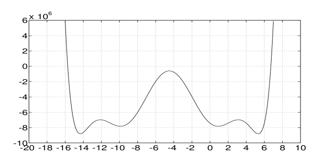
Figure 1. Graph of $P_{m}$ for $m=4$ and $n=n^{*}-1=17$ .

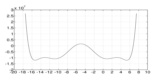
Figure 2. Graph of $P_{m}$ for $m=4$ and $n=n^{*}=18$ .

We recall that in the case $m=2$, the possibility of factorizing $P_{m}$ as a product of four real polynomial of degree 1 was fundamental for proving stability of radial entire solutions of (1) corresponding to the case $\beta\in\partial\mathcal{A}_{\alpha}$, see the proofs of Theorem 6 and Lemma 12 in [6]. The impossibility for $m\geq 4$ even of having a factorization of $P_{m}$ as a product of real polynomials of degree 1 also in dimensions $n\geq n^{*}$ makes difficult to understand if the existence of stable solutions of (1) occurs for such dimensions.

Appendix

In this appendix we recall from [21] and [31] a couple of results concerning solutions of (3): the first one is a result dealing with continuous dependence on initial conditions and the second a comparison principle.

Proposition A.1.

([21]) For any $n\geq 1$ we have:

• for any $\alpha_{0},\dots,\alpha_{m-1}\in\mathbb{R}$ problem (3) admits a unique local solution defined on the maximal interval of continuation $[0,R)$ with $0<R\leq+\infty$;

• let $\alpha_{0},\dots,\alpha_{m-1}\in\mathbb{R}$ and let $\{\alpha_{0,k}\},\dots,\{\alpha_{m-1,k}\}$ sequences in $\mathbb{R}$ such that

  $$\alpha_{0,k}\to\alpha_{0}\,,\qquad\alpha_{i,k}\to\alpha_{i}\quad\text{for any }i\in\{1,\dots,m-1\}\,,\qquad\text{as }k\to+\infty\,.$$

  Denote by $u$ and $u_{k}$ the solutions of (3) corresponding respectively to the initial values $\alpha_{0},\dots,\alpha_{m-1}$ and $\alpha_{0,k},\dots,\alpha_{m-1,k}$. Denote by $[0,R)$, $0<R\leq+\infty$ the maximal interval of continuation of $u$. Then for any $S\in(0,R)$ there exists $\overline{k}>0$ such that for any $k>\overline{k}$, $u_{k}$ is well defined in $[0,S]$ and moreover $u_{k}\to u$ uniformly in $[0,S]$ as $k\to+\infty$.

Proposition A.2.

Assume that $f:\mathbb{R}\rightarrow\mathbb{R}$ is locally Lipschitz continuous and monotonically increasing and let $m\in\mathbb{N}$, $m\geq 1$. Let $u,v\in C^{2m}([0,R))$ be such that

(76) $$\left\{\begin{array}[]{ll}\forall r\in[0,R):\Delta^{m}u(r)-f(u(r))\geq\Delta^{m}v(r)-f(v(r))\,,\\ u(0)\geq v(0)\,,\quad u^{\prime}(0)=v^{\prime}(0)=0\,,\\ \Delta^{k}u(0)\geq\Delta^{k}v(0)\,,\quad(\Delta^{k}u)^{\prime}(0)=(\Delta^{k}v)^{\prime}(0)=0\quad\text{for any }k=1,\dots,m-1\,.\end{array}\right.$$

Then, for all $r\in[0,R)$ and for all $k\in\{1,\dots,m-1\}$ we have

(77) $$u(r)\geq v(r)\,,\quad u^{\prime}(r)\geq v^{\prime}(r)\,,\quad\Delta^{k}u(r)\geq\Delta^{k}v(r)\,,\quad(\Delta^{k}u)^{\prime}(r)\geq(\Delta^{k}v)^{\prime}(r)\,.$$

Moreover, the initial point $0$ can be replaced by any initial point $\rho>0$ if all the four initial data are weakly ordered and a strict inequality in one of the initial data at $\rho\geq 0$ or in the differential inequality in $(\rho,R)$ implies a strict ordering of $u,u^{\prime},\Delta^{k}u,(\Delta^{k}u)^{\prime}$ and $v,v^{\prime},\Delta^{k}v,(\Delta^{k}v)^{\prime}$ on $(\rho,R)$ for any $k\in\{1,\dots,m-1\}$.

Proof. Suppose first that at least one of the inequalities in the differential inequality or in the initial conditions is strict. Then there exist $0<R_{0}\leq R$ and $k\in\{1,\dots,m-1\}$ such that

(78) $$\Delta^{k}u(r)>\Delta^{k}v(r)\qquad\text{for all }r\in(0,R_{0})\,.$$

We may assume that $R_{0}$ is optimal in the sense that

$$R_{0}=\sup\{r\in(0,R):\Delta^{k}u(s)>\Delta^{k}v(s)\ \text{for any }s\in(0,r)\}\,.$$

Suppose by contradiction that $R_{0}<R$.

Writing $\Delta^{k}u(r)=r^{1-n}(r^{n-1}(\Delta^{k-1}u)^{\prime})^{\prime}$ and using the large inequalities in (76), two successive integrations yield

$$(\Delta^{k-1}u(r))^{\prime}>(\Delta^{k-1}v(r))^{\prime}\qquad\text{and}\qquad\Delta^{k-1}u(r)>\Delta^{k-1}v(r)\qquad\text{for all }r\in(0,R_{0})\,.$$

After a finite number of steps we arrive to

$$u(r)>v(r)\qquad\text{for all }r\in(0,R_{0})$$

and hence

$$(r^{n-1}(\Delta^{m-1}u(r))^{\prime})^{\prime} =r^{n-1}\Delta^{m}u(r)\geq r^{n-1}\left[f(u(r))+\Delta^{m}v(r)-f(v(r))\right]$$

$$\geq r^{n-1}\Delta^{m}v(r)=(r^{n-1}(\Delta^{m-1}v(r))^{\prime})^{\prime}\quad\text{for all }r\in(0,R_{0})\,.$$

We can restart the iterative procedure of successive integrations to conclude that the map

$$r\mapsto\Delta^{k}u(r)-\Delta^{k}v(r)$$

is nondecreasing so that by (78) we have $\Delta^{k}u(r)>\Delta^{k}v(r)$ for all $r\in(0,R_{0}]$. The strict inequality until $r=R_{0}$ contradicts the optimality of $R_{0}$. The validity of the inequality (78) in the whole interval $(0,R)$ yields the strict inequalities in the whole $(0,R)$ also for the other terms in (77).

It remains to prove the proposition in the case of large inequalities. To this purpose we consider the unique solution $u_{\varepsilon}$ of the initial value problem

(79) $$\left\{\begin{array}[]{ll}\Delta^{m}u_{\varepsilon}-f(u_{\epsilon})=\Delta^{m}u-f(u)\\ u_{\varepsilon}(0)=u(0)+\varepsilon\,,\quad u^{\prime}_{\varepsilon}(0)=0\\ \Delta^{k}u_{\varepsilon}(0)=\Delta^{k}u(0)\,\quad(\Delta^{k}u_{\varepsilon})^{\prime}(0)=(\Delta^{k}u)^{\prime}(0)\qquad\text{for all }k\in\{1,\dots,m-1\}\,.\end{array}\right.$$

Existence and uniqueness for this initial value problem follows by Proposition A.1 (i).

From the first part of the proof we infer that for any $r\in(0,R)$ and any $\varepsilon>0$

$$u_{\varepsilon}(r)>v(r)\,,\quad u^{\prime}_{\varepsilon}(r)>v^{\prime}(r)\,,$$

$$\Delta^{k}u_{\varepsilon}(r)>\Delta^{k}v(r)\,,\quad(\Delta^{k}u_{\varepsilon})^{\prime}(r)>(\Delta^{k}v)^{\prime}(r)\qquad\text{for any }k\in\{1,\dots,m-1\}\,.$$

Letting $\varepsilon\to 0^{+}$ and using Proposition A.1 (ii) we arrive to the conclusion. We finally observe that the previous argument can be repeated by replacing the initial condition at $r=0$ with an initial condition at any other $\rho\in(0,R)$. $\Box$

Acknowledgement

The authors are grateful to Elvise Berchio for the fruitful discussions during the preparation of this paper.

References

- [1] Adimurthi, Hardy-Sobolev inequality in and its applications, Commun. Contemp. Math. 4 (2002) 409-434.
- [2] W. Allegretto, Nonoscillation theory of elliptic equations of order , Pacific J. Math. 64 (1976) 1-16.
- [3] G. Arioli, F. Gazzola, H.C. Grunau, Entire solutions for a semilinear fourth order elliptic problem with exponential nonlinearity, J. Diff. Eq. 230 (2006) 743-770.
- [4] G. Arioli, F. Gazzola, H.C. Grunau, E. Mitidieri, A semilinear fourth order elliptic problem with exponential nonlinearity, SIAM J. Math. Anal. 36 (2005) 1226-1258.
- [5] H. Brezis, J.L. Vazquez, Blow–up solutions of some nonlinear elliptic problems, Rev. Mat. Univ. Compl. Madrid 10 (1997) 443-469.
- [6] E. Berchio, A. Farina, A. Ferrero, F. Gazzola, Existence and stability of entire solutions to a semilinear fourth order elliptic problem, J. Differential Equations 252 (2012) 2596-2616.
- [7] E. Berchio, F. Gazzola, Some remarks on biharmonic elliptic problems with positive, increasing and convex nonlinearities, Electron. J. Differential Equations 2005 No. 34, 1-20.
- [8] P. Caldiroli, R. Musina, Rellich inequalities with weights, Calc. Var. Partial Differential Equations 45 (1-2) (2012) 147-164.
- [9] S. Chandrasekhar, An introduction to the study of stellar structure, Dover Publ. Inc. 1985.
- [10] S.Y.A. Chang, W. Chen, A note on a class of higher order conformally covariant equations, Discrete Contin. Dyn. Syst. 7 (2001) 275-281.
- [11] E.N. Dancer, A. Farina, On the classification of solutions of on : stability outside a compact set and applications, Proc. Amer. Math. Soc. 137 (4) (2009) 1333-1338.
- [12] E.B. Davies, A.M. Hinz, Explicit constants for Rellich inequalities in , Math. Z. 227 (3) (1998) 511-523.
- [13] J. Dávila, L. Dupaigne, I. Guerra, M. Montenegro, Stable solutions for the bilaplacian with exponential nonlinearity, SIAM J. Math. Anal. 39 (2007) 565-592.
- [14] J. Dávila, I. Flores, I. Guerra, Multiplicity of solutions for a fourth order problem with exponential nonlinearity, J. Differential Equations 247 (2009) 3136-3162.
- [15] J. I. Díaz, M. Lazzo, P. G. Schmidt, Large radial solutions of a polyharmonic equation with superlinear growth, Proceedings of the 2006 International Conference in honor of Jacqueline Fleckinger, 103-128.
- [16] L. Dupaigne, M. Ghergu, O. Goubet, G. Warnault, The Gel’fand problem for the biharmonic operator, Arch. Ration. Mech. Anal. 208 (3) (2013) 725-752.
- [17] A. Farina, Stable solutions of on , C.R.A.S. Paris 345 (2007) 63-66.
- [18] A. Ferrero, H.-Ch. Grunau, The Dirichlet problem for supercritical biharmonic equations with power-type nonlinearity, J. Differential Equations 234 (2007) 582-606.
- [19] A. Ferrero, H.-Ch. Grunau, P. Karageorgis, Supercritical biharmonic equations with power-type nonlinearity, Ann. Mat. Pura Appl. 188 (2009) 171-185.
- [20] A. Ferrero, G. Warnault, On solutions of second and fourth order elliptic equations with power-type nonlinearities, Nonlinear Anal. 70 (8) (2009) 2889-2902.
- [21] B. Franchi, E. Lanconelli, J. Serrin, Existence and uniqueness of nonnegative solutions of quasilinear equations in , Advances in Math. 118 (1996) 177-243.
- [22] F. Gazzola, H.-Ch. Grunau, Radial entire solutions for supercritical biharmonic equations, Math. Ann. 334, (2006) 905-936.
- [23] F. Gazzola, H.C. Grunau, G. Sweers, Polyharmonic boundary value problems, LNM 1991 Springer, 2010.
- [24] I.M. Gel’fand, Some problems in the theory of quasilinear equations, Section 15, due to G.I. Barenblatt, Amer. Math. Soc. Transl. II. Ser. 29 (1963) 295-381. Russian original: Uspekhi Mat. Nauk 14 (1959) 87-158.
- [25] P.L. Lions, On the existence of positive solutions of semilinear elliptic equations, SIAM Rev. 24 (1982) 441-467.
- [26] D. Joseph, T.S. Lundgren, Quasilinear Dirichlet problems driven by positive sources, Arch. Rat. Mech. Anal. 49 (1973) 241-269.
- [27] D. Joseph, E.M. Sparrow, Nonlinear diffusion induced by nonlinear sources, Quart. Appl. Math. 28 (1970) 327-342.
- [28] P. Karageorgis, Stability and intersection properties of solutions to the nonlinear biharmonic equation, Nonlinearity 22 (2009) 1653-1661.
- [29] M. Lazzo, P. G. Schmidt, Radial solutions of a polyharmonic equation with powe nonlinearity, Nonlinear Anal. 71, (2009) 1996-2003.
- [30] C.S. Lin, A classification of solutions of a conformally invariant fourth order equation in , Comment. Math. Helv. 73 (1998) 206-231.
- [31] P.J. McKenna, W. Reichel, Radial solutions of singular nonlinear biharmonic equations and applications to conformal geometry, Electronic J. Differ. Equ. 2003 (37) 1-13.
- [32] L. Martinazzi, Classification of soltions to higher order Liouville’s equation on , Math. Z. 263 (2009) 307-329.
- [33] F. Mignot, J.P. Puel, Sur une classe de problemes non lineaires avec non linearite positive, croissante, convexe, Comm. Part. Diff. Eq. 5 (1980) 791-836.
- [34] E. Mitidieri, A simple approach to Hardy inequalities, Math. Notes 67 (2001) 479-486 translated from Russian.
- [35] E. Mitidieri, S. Pohožaev, A priori estimates and blow-up of solutions to nonlinear partial differential equations and inequalities, Proc. Steklov Inst. Math. 234 (2001) 1-362.
- [36] F. Rellich, Halbbeschränkte Differentialoperatoren höherer Ordnung, (J. C. H. Gerretsen et al. (eds.), Groningen: Nordhoff, 1956), Proceedings of the International Congress of Mathematicians Amsterdam III (1954) 243-250.
- [37] G. Warnault, Liouville theorems for stable radial solutions for the biharmonic operator, Asymptotic Analysis 69, (2010) 87-98.
- [38] J. Wei, D. Ye, Nonradial solutions for a conformally invariant fourth order equation in , Calc. Var. 32 (2008) 373-386.